Superadiabatic dynamical density functional study of Brownian
hard-spheres in time-dependent external potentials

Abstract

Superadiabatic dynamical density functional theory (superadiabatic-DDFT), a first-principles approach based on the inhomogeneous two-body correlation functions, is employed to investigate the response of interacting Brownian particles to time-dependent external driving. Predictions for the superadiabatic dynamics of the one-body density are made directly from the underlying interparticle interactions, without need for either adjustable fit parameters or simulation input. The external potentials we investigate have been chosen to probe distinct aspects of structural relaxation in dense, strongly interacting liquid states. Nonequilibrium density profiles predicted by the superadiabatic theory are compared with those obtained from both adiabatic DDFT and event-driven Brownian dynamics simulation. Our findings show that superadiabatic-DDFT accurately predicts the time-evolution of the one-body density.

I Introduction

Classical Density Functional Theory (DFT) is an exact framework for determining the equilibrium microstructure and thermodynamics of classical many-particle systems in external fields Evans (1979, 1992). The standard method to obtain the one-body density within DFT is to minimize the grand potential functional and solve the resulting Euler-Lagrange (EL) equation for a specified external potential at the temperature and chemical potential of interest. When the grand potential functional is not exactly known, as is usually the case, the EL equation yields density profiles consistent with the compressibility route to the thermodynamics Evans (1992); Tschopp et al. (2022). An alternative approach is provided by the force-DFT in which the same grand potential functional is used to obtain density profiles consistent with the virial route Tschopp et al. (2022). The key feature of force-DFT is that it explicitly uses the inhomogeneous two-body density and exploits the fact that this quantity is a functional of the one-body density. Substitution of the two-body density functional into the well-known Yvon-Born-Green (YBG) equation Hansen and McDonald (2006); McQuarrie (2000) then yields a self-consistent scheme for determining the equilibrium one-body density. Inconsistency between the compressibility and virial routes is familiar from integral equation theories of bulk fluids Caccamo (1996). Standard DFT and force-DFT present an analogous situation on the level of the inhomogeneous one-body density profile, as discussed in detail in reference Tschopp et al. (2022).

The simplest generalization of DFT to treat nonequilibrium Brownian systems is known as the dynamical density functional theory (DDFT). In analogy with equilibrium DFT there are two operationally distinct, but formally equivalent, variations of DDFT. While both of these are based on the assumption that the nonequilibrium two-body density can be represented by the equilibrium two-body density corresponding to the instantaneous nonequilibrium one-body density, they differ in how this ‘adiabatic approximation’ is implemented.

Within standard DDFT the dynamics of the one-body density are driven by the gradient of the one-body direct correlation function Evans (1979); Marconi and Tarazona (1999); Archer and Evans (2004), whereas the force-DDFT involves explicit integration of the adiabatic two-body density to obtain the average interaction force at each time-step Tschopp et al. (2022). Although these approaches often yield qualitatively reasonable results, they are not quantitatively reliable and can break down completely in situations for which the time-evolution of the microstructure involves strongly correlated particle motion Marconi and Tarazona (1999); te Vrugt, Löwen, and Wittkowski (2020).

Very recently a first-principles superadiabatic-DDFT has been developed and implemented Tschopp and Brader (2022). This new approach yields the leading order correction to the adiabatic approximation by explicitly addressing the nonequilibrium dynamics of the inhomogeneous two-body density. The improved resolution provided by the two-body correlations allows for a more realistic description of structural relaxation in strongly interacting systems. Superadiabatic-DDFT does not involve an explicit memory kernel, but rather encodes the history of the system into the current values of the one- and two-body density. The time-evolution of these quantities is determined by the simultaneous solution of a pair of coupled, time-local differential equations. By identifying the one- and two-body density as relevant variables the superadiabatic-DDFT enables a self-contained, autonomous description of many-body Brownian dynamics, which captures the dominant physical processes in the system. Explicit treatment of the inhomogeneous two-body density provides detailed information about the internal structure of the fluid, from which integrated quantities such as the stress tensor (Irving and Kirkwood, 1950; Aerov and Krüger, 2014) or one-body current can be calculated at any point of the time-evolution.

In reference Tschopp and Brader (2022) the superadiabatic-DDFT was derived by a systematic coarse-graining of the many-body Smoluchowski equation. As a first application, this approach was used to predict the time-evolution of the one-body density profile of hard-spheres following an instantaneous change in the external potential. The agreement between the theoretical density profiles and the Brownian dynamics simulation data was very promising. In this paper we continue our investigation of the superadiabatic-DDFT by considering systems driven out-of-equilibrium by the application of a periodically varying time-dependent external potential. The two situations considered have been carefully selected to probe distinct aspects of structural rearrangement in dense fluids. Particular attention will be paid to the transient dynamics of the one-body density in going from equilibrium to the steady-state. The results from superadiabatic-DDFT will be compared with those from force-DDFT, which provides the appropriate reference theory for assessing superadiabatic effects, and event-driven Brownian dynamics (BD) simulation, where the simulations were performed following the algorithm proposed in Ref. Scala, Voigtmann, and De Michele (2007).

II Theory

II.1 Microscopic dynamics

For a system of $N$ interacting Brownian particles the time-evolution of the configurational probability density, $P({\mathbf{r}}^{N}\!,t)$, where ${\mathbf{r}}^{N}$ represents the set of all coordinates, is given by the Smoluchowski equation Dhont (1996)

$$\frac{1}{D_{0}}\frac{\partial P({\mathbf{r}}^{N}\!,t)}{\partial t}=\sum_{i=1}^{N}\nabla_{\mathbf{r}_{i}}\cdot\Big{(}P({\mathbf{r}}^{N}\!,t)\big{(}\nabla_{\mathbf{r}_{i}}\ln(P({\mathbf{r}}^{N}\!,t))\\ +\nabla_{\mathbf{r}_{i}}\beta U({\mathbf{r}}^{N}\!,t)\big{)}\Big{)},$$ (1)

where $\beta\!=\!(k_{B}T)^{-1}$ and $D_{0}$ is the bare diffusion coefficient. For systems with pairwise interactions the total potential energy is given by

$$U({\mathbf{r}}^{N}\!,t)=\sum_{i<j}^{N}\phi(r_{ij})+\sum_{i=1}^{N}V_{\text{ext}}({\mathbf{r}}_{i},t),$$ (2)

where $\phi$ is the pair potential, $r_{ij}=|\mathbf{r}_{i}-\mathbf{r}_{j}|$ and $V_{\text{ext}}$ is a time-dependent external potential.

II.2 Superadiabatic-DDFT

The superadiabatic-DDFT, presented in reference Tschopp and Brader (2022), consists of a pair of differential equations for the coupled time-evolution of the one- and two-body densities. The first equation is obtained by integrating the Smoluchowski equation (1) over $N\!-\!1$ particle coordinates. This yields

$$\frac{1}{D_{0}}\frac{\partial\rho(\mathbf{r}_{1},t)}{\partial t}= \,\nabla_{\mathbf{r}_{1}}\!\!\cdot\!\Bigg{(}\!\nabla_{\mathbf{r}_{1}}\rho(\mathbf{r}_{1},t)+\rho(\mathbf{r}_{1},t)\nabla_{\mathbf{r}_{1}}\beta V_{\text{ext}}(\mathbf{r}_{1},t)$$

$$+\int d\mathbf{r}_{2}\,\rho^{(2)}(\mathbf{r}_{1},\mathbf{r}_{2},t)\nabla_{\mathbf{r}_{1}}\beta\phi(r_{12})\!\Bigg{)},$$ (3)

which is an exact equation of motion for the one-body density, $\rho$, requiring as input the nonequilibrium two-body density, $\rho^{(2)}$.

Integrating the Smoluchowski equation (1) over $N\!-\!2$ particle coordinates yields a formally exact equation of motion for the two-body density. This includes an integral term involving the nonequilibrium three-body density, which is an unknown quantity. However, by invoking an adiabatic closure the full integral term can be approximated using the two-body density Tschopp and Brader (2022). The resulting approximate equation of motion, which constitutes the second equation of superadiabatic-DDFT, is given by

$$\frac{1}{D_{0}}\,\frac{\partial\rho^{(2)}(\mathbf{r}_{1},\mathbf{r}_{2},t)}{\partial t}=$$ (4)

$$\sum_{i=1,2}\nabla_{\mathbf{r}_{i}}\!\cdot\!\Bigg{(}\!\nabla_{\mathbf{r}_{i}}\rho^{(2)}_{\text{\,sup}}(\mathbf{r}_{1},\mathbf{r}_{2},t)\!+\!\rho^{(2)}_{\text{\,sup}}(\mathbf{r}_{1},\mathbf{r}_{2},t)\nabla_{\mathbf{r}_{i}}\beta\phi(r_{12})$$

$$\!\!\!+\!\rho^{(2)}(\mathbf{r}_{1},\mathbf{r}_{2},t)\nabla_{\mathbf{r}_{i}}\beta V_{\text{ext}}(\mathbf{r}_{i})\!-\!\rho^{(2)}_{\text{ad}}(\mathbf{r}_{1},\mathbf{r}_{2},t)\nabla_{\mathbf{r}_{i}}\beta V_{\text{ad}}(\mathbf{r}_{i},t)\!\!\Bigg{)},$$

where the superadiabatic part of the the two-body density is defined according to

$$\rho^{(2)}_{\,\text{sup}}(\mathbf{r}_{1},\mathbf{r}_{2},t)\!\equiv\!\rho^{(2)}(\mathbf{r}_{1},\mathbf{r}_{2},t)-\rho^{(2)}_{\text{ad}}(\mathbf{r}_{1},\mathbf{r}_{2},t)$$ (5)

and where the adiabatic two-body density, $\rho^{(2)}_{\text{ad}}$, is found by evaluating the equilibrium two-body density at the instantaneous one-body density

$$\rho^{(2)}_{\text{ad}}(\textbf{r}_{1},\textbf{r}_{2},t)\equiv\rho^{(2)}_{\text{eq}}(\textbf{r}_{1},\textbf{r}_{2};[\rho(\textbf{r},t)]).$$ (6)

Equation (6) expresses a concept essential for understanding the coupled superadiabatic-DDFT equations (II.2) and (4), namely that the equilibrium two-body density is a functional of the one-body density Tschopp et al. (2020, 2022); Tschopp and Brader (2022). The adiabatic two-body density is obtained by evaluating the equilibrium two-body density functional using the instantaneous nonequilibrium one-body density. The adiabatic potential, $V_{\text{ad}}$, appearing in (4) generates the fictitious external force field required to stabilize the adiabatic system. This is given by the YBG relation of equilibrium statistical mechanics Hansen and McDonald (2006); McQuarrie (2000),

$$-\nabla_{\mathbf{r}_{1}}V_{\text{ad}}(\mathbf{r}_{1},t)\equiv k_{B}T\,\nabla_{\mathbf{r}_{1}}\ln\rho(\mathbf{r}_{1},t)\\ +\int d\mathbf{r}_{2}\,\frac{\rho_{\text{ad}}^{(2)}(\mathbf{r}_{1},\mathbf{r}_{2},t)}{\rho(\mathbf{r}_{1},t)}\nabla_{\mathbf{r}_{1}}\phi(r_{12}),$$ (7)

but here applied to the nonequilibrium system.

For given interaction potential and external field the superadiabatic-DDFT predicts the coupled time-evolution of the one- and two-body density, starting from their initial values $\rho({\mathbf{r}}_{1},t\!=\!0)$ and $\rho^{(2)}({\mathbf{r}}_{1},{\mathbf{r}}_{2},t\!=\!0)$. The theory has no adjustable fit parameter and is not dependent on any input from stochastic simulations (the BD simulation data shown later in this work are purely for comparison). Although the superadiabatic theory is not restricted to any particular choice of external field we will focus in this paper on external potentials exhibiting planar geometry, for which the one-body density varies only as a function of a single cartesian coordinate. In this case the equations of superadiabatic-DDFT can be simplified, as discussed in detail in Section III.A. of Reference Tschopp and Brader (2022).

II.3 Equilibrium limit

In equilibrium the term in parentheses on the right hand-side of equation (II.2) vanishes and we obtain the first-order YBG equation

$$\nabla_{\mathbf{r}_{1}}\rho_{\text{eq}}(\mathbf{r}_{1})+\rho_{\text{eq}}(\mathbf{r}_{1})\nabla_{\mathbf{r}_{1}}\beta V_{\text{ext}}(\mathbf{r}_{1})\\ +\int d\mathbf{r}_{2}\,\rho_{\text{eq}}^{(2)}(\mathbf{r}_{1},\mathbf{r}_{2};[\rho_{\text{eq}}])\nabla_{\mathbf{r}_{1}}\beta\phi(r_{12})=0.$$ (8)

The zero-sum of these three terms expresses the equilibrium balance between Brownian, external and internal forces Hansen and McDonald (2006). The notation employed again highlights that the equilibrium two-body density is a unique functional of the one-body density. Of the various methods available to obtain this two-body density functional, the most accurate are those based on solution of the inhomogeneous Ornstein-Zernike (OZ) equation

$$h_{\text{eq}}({\mathbf{r}}_{1},{\mathbf{r}}_{2};[\rho_{\text{eq}}])=c^{(2)}_{\text{eq}}({\mathbf{r}}_{1},{\mathbf{r}}_{2};[\rho_{\text{eq}}])\\ +\int\!d{\mathbf{r}}_{3}\,h_{\text{eq}}({\mathbf{r}}_{1},{\mathbf{r}}_{3};[\rho_{\text{eq}}])\,\rho_{\text{eq}}({\mathbf{r}}_{3})\,c^{(2)}_{\text{eq}}({\mathbf{r}}_{3},{\mathbf{r}}_{2};[\rho_{\text{eq}}]),$$ (9)

where $h_{\text{eq}}$ is the total correlation function and $c^{(2)}_{\text{eq}}$ is the two-body direct correlation function. In this work we choose to follow the approach employed in reference Tschopp and Brader (2022) and calculate $c^{(2)}_{\text{eq}}$ by taking the second functional derivative of the excess (over ideal) Helmholtz free energy functional, $F^{\,\text{exc}}$, with respect to the density

$$c^{(2)}_{\text{eq}}({\mathbf{r}}_{1},{\mathbf{r}}_{2};[\rho_{\text{eq}}])=-{\frac{\delta^{2}\beta F^{\,\text{exc}}[\rho]}{\delta\rho({\mathbf{r}}_{1})\delta\rho({\mathbf{r}}_{2})}}\bigg{\rvert}_{\rho_{\text{eq}}}.$$ (10)

As there exist reliable approximations to $F^{\,\text{exc}}$ for many model systems, we can regard $c^{(2)}_{\text{eq}}$ as a known quantity, such that $h_{\text{eq}}$ can be determined by solution of equation (20). This can then be related to the two-body density according to

$$h_{\text{eq}}({\mathbf{r}}_{1},{\mathbf{r}}_{2};[\rho_{\text{eq}}])=\frac{\rho^{(2)}_{\text{eq}}({\mathbf{r}}_{1},{\mathbf{r}}_{2};[\rho_{\text{eq}}])}{\rho_{\text{eq}}({\mathbf{r}}_{1})\rho_{\text{eq}}({\mathbf{r}}_{2})}-1.$$ (11)

The closed set of equations (8),(20),(10) and (21) constitutes the force-DFT Tschopp et al. (2022), which is the equilibrium limit of superadiabatic-DDFT.

III Results for three-dimensional hard-spheres in planar geometry

The hard-sphere model captures the packing constraints which dominate structural relaxation in dense liquids and thus presents an appropriate choice for the present study. In the following we show numerical results for a three-dimensional system of hard-spheres, of diameter $d\!=\!1$, subject to a time-dependent external potential. The units of energy and time are fixed by $k_{B}T\!=\!1$ and $d^{2}/D_{0}\!=\!1$, respectively. The external potential considered is a function of a single cartesian coordinate, taken here as the $z$-direction, which imposes a planar symmetry. The potential consists of a harmonic trap with an additional (time-dependent) Gaussian peak and takes the following form

$$V_{\text{ext}}(z,t)=A\,\Big{(}z-z_{0}^{A}\Big{)}^{2}+B(t)\,e^{-\alpha\left(z-z_{0}^{B}(t)\right)^{2}},$$ (12)

where the harmonic trap amplitude is set equal to $A\!=\!1.5$ with its minimum located at $z_{0}^{A}\!=\!5$. The Gaussian decay parameter is set to a constant value of $\alpha\!=\!5$, while its amplitude and peak position are given by the time-dependent functions $B(t)$ and $z_{0}^{B}(t)$, respectively. In the following we explore two specific realizations of this general external potential to probe strongly correlated cooperative motion and structural relaxation. The resulting one-body density profiles from superadiabatic-DDFT are then benchmarked against BD simulation data and compared with the predictions of force-DDFT. We calculate the adiabatic two-body density by using equations (20), (10) and (21) together with the well-known Rosenfeld approximation to the excess Helmholtz free energy Rosenfeld (1989) (see Appendix A for further details).

As already mentioned in the introduction, the force-DDFT is a purely adiabatic approach which assumes instantaneous equilibration of the two-body density. Superadiabatic- and force-DDFT have the same equilibrium limit, namely force-DFT, and this convenient feature enables a comparison focused solely on adiabatic/superadiabatic differences, without any residual equilibrium bias. A full account of the force-DDFT method can be found in Reference Tschopp et al. (2022). Implementation details for both superadiabatic- and force-DDFT in planar geometry can be found in Sections III.A. and III.B. of Reference Tschopp and Brader (2022) and in Sections III.G. and IV.A. of Reference Tschopp et al. (2022), respectively.

III.1 Periodic compression

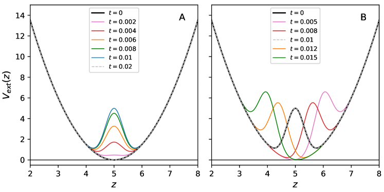
Figure 1: Time-dependent external potentials for the two special cases considered in this work. The general form of the potential is given in equation (12). In panel A, we show a potential consisting of a confining harmonic trap and a centered Gaussian peak with a time-dependent amplitude (see equation (13)). In panel B, we show a potential consisting of the same harmonic trap, but now with a Gaussian peak which moves (with fixed amplitude) back-and-forth about the trap minimum (see equation (14)). The first case is designed to ‘periodically compress’ the particles away from the center and towards the outer regions of the trap. The second case induces more flow in the system, as the Gaussian peak constantly disrupts the particle microstructure.

For our first test-case we set the external potential (12) such that the location of the Gaussian peak is held constant in the center of the harmonic trap, $z_{0}^{B}(t)\!=\!z_{0}^{A}\!=\!5$, with a time-dependent amplitude given by

$$B(t)=\frac{B_{\text{max}}}{2}\Big{(}1-\cos(\omega t)\Big{)},$$ (13)

for $t\!>\!0$ and zero for earlier times. We choose a maximal amplitude $B_{\text{max}}\!=\!5$ and frequency $\omega\!=\!2\pi/0.02$. The time-dependent variation of the external potential is illustrated in panel A of Figure 1.

The system is initially prepared in an equilibrium state with an average of $2.5$ particles per unit area in the $xy$-plane, i.e. $\langle N\rangle\!=\!\int dz\,\rho_{\rm eq}(z)\!=\!2.5$, before being driven out-of-equilibrium by the oscillatory Gaussian peak (13) for times $t\!>\!0$. Panels B to E of Figure 2 show theoretical density profiles at different times, calculated using both superadiabatic-DDFT (red-framed panels C and E) and force-DDFT (green-framed panels B and D). The data shown in Panel A tracks the value of the one-body density at the center of the harmonic trap, $\rho(z\!=\!5,t)$, as a function of time. This shows clearly the transient relaxation of the one-body density from equilibrium to a periodic nonequilibrium steady-state. The filled circles indicate times at which we show the full density profile in panels B to E and the stars are results of BD simulation, shown at regular time intervals.

We first discuss the data shown in Panel A of Figure 2. At time $t\!=\!0$ the system is in equilibrium and both superadiabatic- and force-DDFT predict identical density profiles, namely those of force-DFT. The equilibrium density profile is not in perfect agreement with that of simulation (calculated using the Monte-Carlo method) due to the approximate free energy used to calculate the equilibrium two-body density, in analogy with the situation considered in reference Tschopp and Brader (2022). From $t\!=\!0$ until around $t\!=\!0.2$ we observe a transient relaxation during which $\rho(z\!=\!5,t)$ decreases after each oscillation period. This decrease reflects the changes in the microstructure caused by periodically compressing the particles away from the center and towards the outer regions of the harmonic trap. During the transient regime, interparticle collisions cause the particles to adjust their positions in such a way that they can move as freely as possible back-and-forth in response to the externally applied forces. The time-dependent Gaussian respects the symmetry of the trap (mirror symmetric about $z\!=\!5$) and does not induce a large amount of flow, but rather leads to more subtle configurational changes as each particle modifies its local environment through repeated interaction with its neighbours. The absence of strong flow in the system suggests that superadiabatic effects can be expected to be modest. The superadiabatic- and force-DDFT predictions for $\rho(z\!=\!5,t)$ are given by the red and green curves, respectively. The prediction of superadiabatic-DDFT is in excellent quantitative agreement with the BD data and captures almost perfectly the transient behaviour, whereas the force-DDFT decays too rapidly. The superadiabatic-DDFT correctly implements the zero flux condition on the two-body density at all times and thus provides a much more realistic account of the microstructural rearrangements induced by external forces.

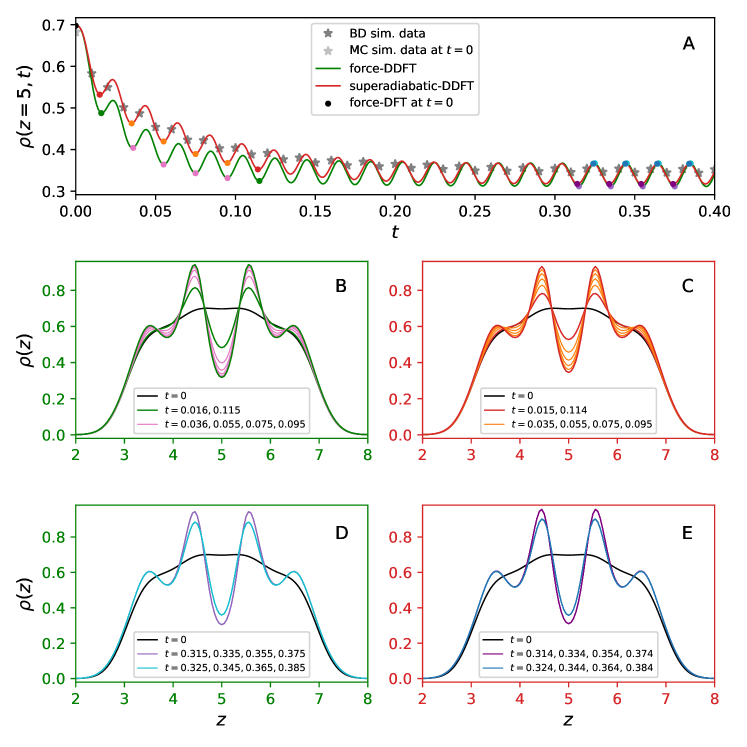
Figure 2: Periodic compression. Starting from the equilibrium density profile in a harmonic trap we track the time-evolution of the one-body density following the switch-on (at $t\!=\!0$) of an additional repulsive Gaussian potential with a time-dependent amplitude, see equations (12) and (13). Panel A shows the density at the trap center ($z\!=\!5$) as a function of time obtained from superadiabatic-DDFT (red line) and force-DDFT (green line). The stars are data points from simulation and the filled circles indicate the times at which we show full density profiles in Panels B to E (note the corresponding colour scheme). Following a period of transient relaxation the system enters a periodic stationary state for times greater than $t\!\sim\!0.2$.

In Panels B and C we show the full one-body density profiles from force- and superadiabatic-DDFT, respectively, at selected times during the transient relaxation. These times (indicated by filled circles in Panel A) have been selected such that force- and superadiabatic-DDFT profiles can be compared at equivalent points in the oscillation cycle, rather than at strictly equal times. As the repulsive Gaussian peak grows in magnitude (see Figure 1), particles are forced away from the center of the harmonic trap and a first packing peak develops on either side of the trap minimum. Although qualitatively similar, this process occurs more slowly in superadiabatic-DDFT than in force-DDFT, which we attribute to the improved treatment of structural relaxation in the superadiabatic theory, as discussed above. As the system approaches a steady-state, the density profile develops a second packing peak on either side of the trap minimum. Here we again observe that the build-up of packing structure takes longer in superadiabatic-DDFT than in force-DDFT.

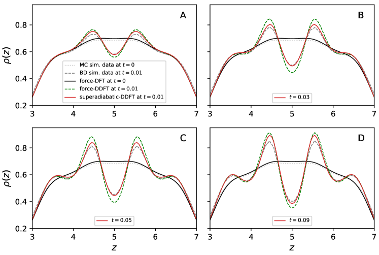
Figure 3: Periodic compression. Comparing the predictions of force- and superadiabatic-DDFT (green dashed lines and red solid lines, respectively) with BD simulation data (gray dashed lines) at four different times during the transient time-evolution of the system. The external potential is given by (12) and (13) and generates a periodic compression of the particles towards the sides of the harmonic trap. The equilibrium density curves, at $t\!=\!0$, obtained by force-DFT (black solid lines) and Monte-Carlo simulation (silver dottd lines) are included as a reference. In all cases the superadiabatic-DDFT agrees considerably better with the simulation data than the force-DDFT.

Returning to panel A, the value of the one-body density at the trap minimum, $\rho(z\!=\!5,t)$, indicates the onset of a steady-state for times $t\!>\!0.2$. In Panel E we show full density profiles calculated in this steady-state using superadiabatic-DDFT at times separated by one oscillation period. The purple coloured profiles were calculated at minima of the curve shown in Panel A, whereas the blue profiles were calculated at the maxima. The fact that curves of the same colour cannot be distinguished from each other confirms that we have indeed entered a steady-state for the full density profile and not only for its value at $z\!=\!5$. The same conclusion can be drawn from the profiles calculated using force-DDFT shown in Panel D. The strong similarity between the steady-state profiles calculated using both force- and superadiabatic-DDFT (compare, for example, the light and dark purple curves in Panels D and E, respectively) is a consequence of a nonequilibrium microstructure which allows each particle to oscillate locally back-and-forth without very frequent interaction with its neighbours. In such a state, one can expect that superadiabatic effects, which arise from interparticle interactions, will remain small. It is thus not surprising that the steady-state density profiles of force- and superadiabatic-DDFT are in close agreement. This does not apply to the transient regime, during which frequent interparticle interactions serve to break-up and rearrange the initial equilibrium microstructure. We note that superadiabatic effects will have an increased influence on the steady-state density profiles in more densely packed systems with a larger value of $\langle N\rangle$, but we choose to focus here on fluid states at more moderate packing.

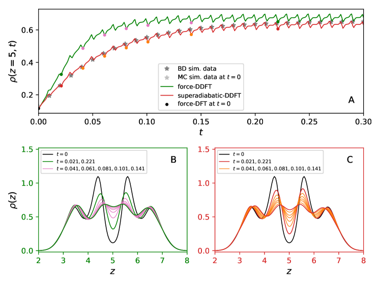
Figure 4: Flow induced mixing. Starting, at $t\!=\!0$, with the equilibrium density profile in a harmonic trap with a fixed Gaussian peak at $z_{0}^{B}\!=\!z_{0}^{A}\!=\!5$, we show, for $t\!\geq\!0$, the time-evolution of the one-body density as the Gaussian peak sweeps from side-to-side following equations (12) and (14). Panel A shows values of the density at the trap center ($z\!=\!5$) as a function of time obtained from superadiabatic-DDFT (red line) and force-DDFT (green line). The stars are data points from simulation and the filled circles indicate the times at which we show full density profiles within the transient regime in Panels B (force-DDFT) and C (superadiabatic-DDFT) - note the corresponding colour scheme.

In Figure 3 we compare the predictions of force- and superadiabatic-DDFT with simulation data at four different times during the transient regime of the time evolution. The superadiabatic-DDFT is globally more accurate than force-DDFT at all times. However, agreement with the simulation data is still not perfect. We attribute much of the error exhibited by superadiabatic-DDFT to the underlying equilibrium free energy functional used to generate the adiabatic two-body density (see equation (10)). The deviation of the equilibrium force-DFT curve at $t\!=\!0$ from the Monte-Carlo data persists in the nonequilibrium density profiles from superadiabatic-DDFT, which is consistent with the findings of reference Tschopp and Brader (2022). We are confident that employing a more accurate equilibrium approximation to generate the adiabatic two-body density would enable the superadiabatic-DDFT to give an even more satisfactory account of the simulation data. In any case, this residual equilibrium error becomes less significant when the system undergoes stronger flow and superadiabatic effects become more prominent, as demonstrated below.

III.2 Flow induced mixing

We next set the external potential (12) such that the Gaussian has a constant amplitude, $B(t)\!=\!B_{\text{max}}\!=\!5$, but a time-dependent position, given by

$$z_{0}^{B}(t)=\begin{cases}z_{0}^{A},&\text{if $t<0$}\\ z_{0}^{A}+\Delta z\sin(\omega t),&\text{if $t\geq 0$}\end{cases}$$ (14)

where $\Delta z\!=\!1$ is the maximal displacement of the Gaussian peak away from the harmonic potential minimum, located at $z_{0}^{A}\!=\!5$, and where we have again taken the frequency $\omega\!=\!2\pi/0.02$. The time-dependent variation of this external potential is shown in panel B of Figure 1. The system is initially prepared in an equilibrium state with an average of 2.5 particles per unit area in the $xy$-plane and is then driven out-of-equilibrium by the side-to-side oscillatory motion of the Gaussian peak.

We begin by discussing Panel A of Figure 4, which shows the value of the one-body density at the center of the harmonic trap, $\rho(z\!=\!5,t)$, as a function of time. The green and red curves show the predictions of force- and superadiabatic-DDFT, respectively, where both theories predict a regime of transient relaxation before arriving at a nonequilibrium steady-state. The stars are data from simulation, sampled at regularly spaced time intervals, and the filled circles indicate the times at which we show full density profiles in Panels B and C. The predictions of force- and superadiabatic-DDFT shown in Panel A reveal much greater discrepancy between the two theories than in the previously considered test-case (see Figure 2). The superadiabatic-DDFT is once again in very good agreement with the BD simulation data and gives an accurate description of both the transient relaxation and the steady-state. In contrast, the transient predicted by force-DDFT decays too rapidly and stabilizes to an erroneous steady-state.

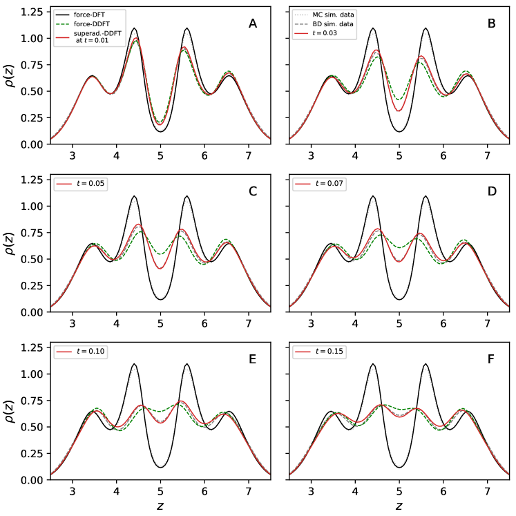
Figure 5: Flow induced mixing. Panels A to F compare theoretical predictions with BD simulation data at different times during the transient regime. In each Panel we give equilibrium profiles from force-DFT, black solid lines, and Monte-Carlo simulation, silver dotted lines, to serve as a reference. Force-DDFT profiles are given by green dashed lines, superadiabatic-DDFT profiles by red solid lines and BD simulation data by dashed gray lines.

While force-DDFT performs rather poorly, giving at best a qualitative description, the superadiabatic-DDFT gives an excellent quantitative account of the BD data and captures very well the time-scale of transient relaxation. The sweeping, back-and-forth motion of the Gaussian peak induces a global flow, involving frequent interparticle collisions, which mixes the particles as they repeatedly flow over the moving potential barrier. This continual, global disturbance of the microstructure causes the nonequilibrium two-body density to deviate significantly from the adiabatic two-body density and thus generates strong superadiabatic effects. While the differences between the two theories are most pronounced during the transient, they are still apparent in the steady-state, where the particles continue to undergo numerous collisions as they are forced to move back-and-forth past their neighbours. This situation should be contrasted with the steady-state of the previous test-case, where superadiabatic effects were found to be small (see Figure 2) due to the relatively unhindered, small-amplitude, oscillatory motion of each particle within its own local environment.

Panels B and C of Figure 4 show theoretical density profiles at different times, calculated using both force-DDFT (green-framed panel B) and superadiabatic-DDFT (red-framed panel C). The times chosen are indicated by the filled circles in Panel A, where we note the matching colour scheme between the points and the full density profiles. Due to the oscillatory motion of the Gaussian peak, which initially moves to the right following the onset of motion at $t\!=\!0$, the density profiles are asymmetric about the minimum of the Gaussian trap. Consistent with our previous findings the superadiabatic-DDFT reacts slower to changes in the external field than the force-DDFT, e.g. the central minimum in the equilibrium profile is more slowly eroded by the motion of the Gaussian peak. Indeed, for the later times shown the force-DDFT profiles are almost overlapping, reflecting the onset of the steady-state, whereas the corresponding superadiabatic-DDFT profiles can be easily distinguished from each other.

In Figure 5 we compare density profiles predicted by superadiabatic- and force-DDFT with BD simulation data. As a reference for the eye, we also show the starting equilibrium curves from force-DFT and Monte-Carlo simulation. In this figure, it is clear that the nonequilibrium density profiles predicted by superadiabatic-DDFT are in remarkably good agreement with the simulation data and capture with high accuracy the global shape of the profiles at all times considered. In contrast, force-DDFT is not able to describe the time-evolution of the profiles in a satisfactory way and yields a generally poor account of the packing oscillations.

In this second test-case, the improvement of superadiabatic-DDFT over force-DDFT is much more dramatic than in the previous test-case, since the superadiabatic forces, closely linked to the particle packing, stay relevant even into the steady-state regime. For such dynamics explicitly including the time-evolution of the two-body density is very important to describe accurately the microstructural changes in the driven system.

IV Discussion and conclusions

In this paper the recently developed superadiabatic-DDFT Tschopp and Brader (2022) was used to study the dynamics of a system of hard-spheres subject to a time-dependent external field. Our results show that superadiabatic-DDFT provides an accurate description of structural relaxation in fluids and reveal clearly the deficiencies of the more simplistic force-DDFT method Tschopp et al. (2022).

Within the force-DDFT the adiabatic two-body density is calculated at each time-step and used to generate the one-body force due to interparticle interactions. However, an undesirable consequence of applying the adiabatic approximation at the one-body level is that both $\rho$ and $\rho^{(2)}_{\text{ad}}$ follow an unphysical time-evolution, which does not respect the packing constraints imposed by interaction potentials with a strong short-range repulsion. More concretely, if we consider the time-evolution of the full many-particle system, as calculated in BD simulation, then the functions $\rho$ and $\rho^{(2)}_{\text{ad}}$ predicted by force-DDFT could not be obtained from statistical averages over a physically realistic sequence of configurations. Even if it were possible to reproduce these functions by back-engineering some artifical configuration sequence, then this would likely involve unphysical situations for which the particles overlap. In contrast, the superadiabatic-DDFT prevents such unphysical overlaps, due to the explicit (non-integrated) appearance of the pair interaction potential in equation (4). The error in superadiabatic-DDFT lies in the neglect of subtle differences between higher-order correlations of the adiabatic and nonequilibrium systems.

An alternative framework for treating superadiabatic dynamics is provided by the power functional theory (PFT) Schmidt and Brader (2013); Schmidt (2022), which formally generalizes the variational approach of DFT to nonequilibrium. Within PFT all superadiabatic effects are described by an excess power functional with a nonlocal dependence on the entire history of both the one-body density and current. In principle, knowledge of this excess functional would provide a closed, predictive theory for the dynamics of the one-body density. However, in practice, the complexity of the excess functional has prevented the construction of any approximation capable of providing this closure. The fact that PFT requires a temporally nonlocal excess power functional is a natural consequence of using the one-body density and current as relevant variables. The information lost in coarse-graining to these one-body fields is compensated by the use of memory kernels, which are generally difficult to approximate. The superadiabatic-DDFT approach employed in this work identifies the one- and two-body densities as the relevant variables for a coarse-grained description of many-body Brownian dynamics. This provides detailed information about the microstructure of the nonequilibrium fluid and enables the formulation of a closed, time-local dynamical theory. Within superadiabatic-DDFT the flow history of the system is encoded in the current value of the nonequilibrium two-body density, without the need for a memory kernel.

Since collective motion in dense fluids, whether in- or out-of-equilibrium, is dominated by the repulsive part of the interparticle interaction potential, we chose in the present work to focus on the three-dimensional hard-sphere model. However, we emphasise that our approach is by no means limited to hard-spheres and can be applied without difficulty to systems interacting via any pairwise additive interaction potential.

Two different time-dependent external potentials were considered. In the first case the external field generated a local, periodic compression of the system for which superadiabatic effects are expected to be modest, such that the steady-states predicted by superadiabatic- and force-DDFT are very similar. This enabled us to focus solely on the transient regime and demonstrate the improved performance of the superadiabtic-DDFT over force-DDFT. In the second case the external field induced a global flow in the system, which generates strong superadiabatic effects in both the transient regime and the steady-state. We again found that the superadiabatic-DDFT predicts one-body density profiles in very good agreement with the BD simulation data and performs far better than the force-DDFT.

We thus conclude that superadiabatic-DDFT provides a reliable and accurate method to predict the dynamics of the one-body density in systems driven by time-dependent external potentials.

Data Availability

The data that support the findings of this study are available from the corresponding author upon reasonable request.

Appendix A FMT for the two-body density

Within the fundamental measure theory (FMT) the excess Helmholtz free energy functional is approximated by an integral over a function of weighted densities Rosenfeld (1989)

$$\beta F^{\text{exc}}_{\text{hs}}[\,\rho\,]=\int\!d{\mathbf{r}}_{1}\;\Phi\left(\left\{n_{\alpha}({\mathbf{r}}_{1})\right\}\right).$$ (15)

The original Rosenfeld version of FMT employs the following approximate form for the reduced excess free energy density of the hard-sphere system

$$\Phi=-n_{0}\ln(1-n_{3})+\frac{n_{1}n_{2}-\mathbf{n}_{1}\cdot\mathbf{n}_{2}}{1-n_{3}}+\frac{n_{2}^{3}-3n_{2}\mathbf{n}_{2}\cdot\mathbf{n}_{2}}{24\pi(1-n_{3})^{2}}.$$ (16)

The weighted densities are generated by convolution

$$n_{\alpha}({\mathbf{r}}_{1})=\int\!d{\mathbf{r}}_{2}\;\rho({\mathbf{r}}_{2})\,\omega_{\alpha}({\mathbf{r}}_{12}),$$ (17)

where ${\mathbf{r}}_{12}\!=\!{\mathbf{r}}_{1}\!-\!{\mathbf{r}}_{2}$ and the weight functions, $\omega_{\alpha}$, are given by four scalar functions

$$\omega_{3}({\mathbf{r}}) =\Theta(R-|{\mathbf{r}}|),\hskip 14.22636pt\omega_{2}({\mathbf{r}})=\delta(R-|{\mathbf{r}}|),$$

$$\omega_{1}({\mathbf{r}}) =\frac{\delta(R-|{\mathbf{r}}|)}{4\pi R},\hskip 15.36429pt\omega_{0}({\mathbf{r}})=\frac{\delta(R-|{\mathbf{r}}|)}{4\pi R^{2}},$$

and two vectors

$$\omega_{\mathbf{2}}({\mathbf{r}}) =\mathbf{e}_{{\mathbf{r}}}\,\delta(R-|{\mathbf{r}}|),\hskip 15.6491pt\omega_{\mathbf{1}}({\mathbf{r}})=\mathbf{e}_{{\mathbf{r}}}\frac{\delta(R-|{\mathbf{r}}|)}{4\pi R},$$

where $\mathbf{e}_{{\mathbf{r}}}\!=\!{\mathbf{r}}/|{\mathbf{r}}|$ is a unit vector. The symbol $\omega$ is used here for all weight functions, with vector functions distinguished from scalar functions by using a bold font index, in accordance with the notation introduced in Ref. Tschopp and Brader (2021).

Within DFT the equilibrium two-body direct correlation function is obtained by taking two functional derivatives of the excess Helmholtz free energy, as given in equation (10). When applied to the approximate Rosenfeld expression (15) this yields Tschopp and Brader (2021)

$$c^{(2)}_{\text{eq}}({\mathbf{r}}_{1},{\mathbf{r}}_{2};[\,\rho_{\text{eq}}\,])=-\!\sum_{\alpha\beta}\int\!d{\mathbf{r}}_{3}\,\omega_{\alpha}({\mathbf{r}}_{31})\,\Phi^{{}^{\prime\prime}}_{\alpha\beta}({\mathbf{r}}_{3})\,\omega_{\beta}({\mathbf{r}}_{32}),$$ (18)

where $\Phi^{{}^{\prime\prime}}_{\alpha\beta}\!=\!\partial^{2}\Phi/\partial n_{\alpha}\partial n_{\beta}$ and the sums over $\alpha$ and $\beta$ run over all scalar and vector indices. From equations (16), (17) and (18) it is clear that the two-body direct correlation function is determined purely by the one-body density. Substitution of a nonequilibrium one-body density into the expression (18) generates the adiabatic two-body direct correlation function

$$c^{(2)}_{\text{ad}}({\mathbf{r}}_{1},{\mathbf{r}}_{2},t)\equiv c^{(2)}_{\text{eq}}({\mathbf{r}}_{1},{\mathbf{r}}_{2};[\rho(\textbf{r},t)]).$$ (19)

Substitution of $c^{(2)}_{\text{ad}}$ into the inhomogeneous OZ equation

$$h_{\text{ad}}({\mathbf{r}}_{1},{\mathbf{r}}_{2},t)=c^{(2)}_{\text{ad}}({\mathbf{r}}_{1},{\mathbf{r}}_{2},t)\\ +\int\!d{\mathbf{r}}_{3}\,h_{\text{ad}}({\mathbf{r}}_{1},{\mathbf{r}}_{3},t)\,\rho({\mathbf{r}}_{3},t)\,c^{(2)}_{\text{ad}}({\mathbf{r}}_{3},{\mathbf{r}}_{2},t),$$ (20)

yields the adiabatic total correlation function $h_{\text{ad}}$, from which the adiabatic two-body density can easily be found using

$$\rho^{(2)}_{\text{ad}}({\mathbf{r}}_{1},{\mathbf{r}}_{2},t)=\rho({\mathbf{r}}_{1},t)\rho({\mathbf{r}}_{2},t)\big{(}\,h_{\text{ad}}({\mathbf{r}}_{1},{\mathbf{r}}_{2},t)+1\,\big{)}.$$ (21)

We refer the reader to Ref. Tschopp and Brader (2021) for details of how to implement the above scheme in cases for which the one-body density has either planar or spherical symmetry.

References

References

- Evans (1979) R. Evans, “The nature of the liquid-vapour interface and other topics in the statistical mechanics of non-uniform, classical fluids,” Advances in Physics 28, 143–200 (1979).
- Evans (1992) R. Evans, Ch. 3 in Fundamentals of Inhomogeneous Fluids, D. Henderson, ed., Marcel Dekker, New York (1992).
- Tschopp et al. (2022) S. M. Tschopp, F. Sammüller, S. Hermann, M. Schmidt, and J. M. Brader, “Force density functional theory in- and out-of-equilibrium,” Phys. Rev. E 106, 014115 (2022).
- Hansen and McDonald (2006) J. Hansen and I. McDonald, Theory of Simple Liquids (Elsevier Science, 2006).
- McQuarrie (2000) D. McQuarrie, Statistical Mechanics (University Science Books, 2000).
- Caccamo (1996) Caccamo, “Integral equation theory description of phase equilibria in classical fluids,” Physics Reports 274, 1–105 (1996).
- Marconi and Tarazona (1999) U. M. B. Marconi and P. Tarazona, “Dynamic density functional theory of fluids,” The Journal of Chemical Physics 110, 8032–8044 (1999).
- Archer and Evans (2004) A. J. Archer and R. Evans, “Dynamical density functional theory and its application to spinodal decomposition,” J. Chem. Phys. 121, 4246–4254 (2004).
- te Vrugt, Löwen, and Wittkowski (2020) M. te Vrugt, H. Löwen, and R. Wittkowski, “Classical dynamical density functional theory: from fundamentals to applications,” Advances in Physics 69, 121–247 (2020).
- Tschopp and Brader (2022) S. M. Tschopp and J. M. Brader, “First-principles superadiabatic theory for the dynamics of inhomogeneous fluids,” The Journal of Chemical Physics 157, 234108 (2022).
- Irving and Kirkwood (1950) J. H. Irving and J. G. Kirkwood, “The statistical mechanical theory of transport processes. iv. the equations of hydrodynamics,” The Journal of Chemical Physics 18, 817–829 (1950).
- Aerov and Krüger (2014) A. A. Aerov and M. Krüger, “Driven colloidal suspensions in confinement and density functional theory: Microstructure and wall-slip,” The Journal of Chemical Physics 140, 094701 (2014).
- Scala, Voigtmann, and De Michele (2007) A. Scala, T. Voigtmann, and C. De Michele, “Event-driven brownian dynamics for hard spheres,” The Journal of Chemical Physics 126, 134109 (2007), https://doi.org/10.1063/1.2719190 .
- Dhont (1996) J. Dhont, An Introduction to Dynamics of Colloids (Elsevier Science, 1996).
- Tschopp et al. (2020) S. M. Tschopp, H. D. Vuijk, A. Sharma, and J. M. Brader, “Mean-field theory of inhomogeneous fluids,” Phys. Rev. E 102, 042140 (2020).
- Rosenfeld (1989) Y. Rosenfeld, “Free-energy model for the inhomogeneous hard-sphere fluid mixture and density-functional theory of freezing,” Phys. Rev. Lett. 63, 980 (1989).
- Schmidt and Brader (2013) M. Schmidt and J. M. Brader, The Journal of Chemical Physics 138, 214101 (2013).
- Schmidt (2022) M. Schmidt, Rev. Mod. Phys. 94, 015007 (2022).
- Tschopp and Brader (2021) S. M. Tschopp and J. M. Brader, Phys. Rev. E 103, 042103 (2021)..