Strichartz estimates for the Schrödinger equation on negatively curved compact manifolds

Abstract.

We obtain improved Strichartz estimates for solutions of the Schrödinger equation on negatively curved compact manifolds which improve the classical universal results results of Burq, Gérard and Tzvetkov [11] in this geometry. In the case where the spatial manifold is a hyperbolic surface we are able to obtain no-loss $L^{q_{c}}_{t,x}$-estimates on intervals of length $\log\lambda\cdot\lambda^{-1}$ for initial data whose frequencies are comparable to $\lambda$, which, given the role of the Ehrenfest time, is the natural analog of the universal results in [11]. We are also obtain improved endpoint Strichartz estimates for manifolds of nonpositive curvature, which cannot hold for spheres.

1. Introduction

It has been almost two decades since Burq, Gérard and Tzvetkov [11] obtained their now classical universal Strichartz estimates for the Schrödinger equation on compact manifolds. Besides the notable exception of near lossless estimates on general tori by Bourgain and Demeter [10], and more recent related work in this setting by Deng, Germain and Guth [13] and Deng, Germain, Guth and Meyerson [14], to the best of our knowledge, there have not been significant improvements of the results in [11], in other geometries.

The purpose of this paper is to obtain improvement of the universal bounds in [11] under the assumption of negative curvature, as well as, more generally, nonpositive curvature.

Let us now recall the universal estimates of Burq, Gérard and Tzvetkov [11]. If $(M^{d},g)$ is a compact Riemannian manifold of dimension $d\geq 2$, then the main estimate in [11] is that if $\Delta_{g}$ is the associated Laplace-Beltrami operator and

(1.1) $$u(x,t)=\bigl{(}e^{-it\Delta_{g}}f\bigr{)}(x)$$

is the solution of the Schrödinger equation on $M^{d}\times{\mathbb{R}}$,

(1.2) $$i\partial_{t}u(x,t)=\Delta_{g}u(x,t),\quad u(x,0)=f(x),$$

then one has the mixed-norm Strichartz estimates

(1.3) $$\|u\|_{L^{p}_{t}L^{q}_{x}(M^{d}\times[0,1])}\lesssim\|f\|_{H^{1/p}(M^{d})}$$

for all admissible pairs $(p,q)$. By the latter we mean, as in Keel and Tao [21],

(1.4) $$d(\tfrac{1}{2}-\tfrac{1}{q})=\tfrac{2}{p}\,\,\,\text{and }\,\,2<q\leq\tfrac{2d}{d-2}\,\,\text{if }\,d\geq 3,\,\,\,\text{or }\,2<q<\infty\,\,\text{if }\,\,d=2.$$

Also, in (1.3) $H^{\mu}$ denotes the standard Sobolev space

(1.5) $$\|f\|_{H^{\mu}(M^{d})}=\bigl{\|}\,(I+P)^{\mu}f\,\bigr{\|}_{L^{2}(M^{d})},\quad\text{with }\,\,P=\sqrt{-\Delta_{g}},$$

and “$\lesssim$” in (1.3) and, in what follows, denotes an inequality with an implicit, but unstated, constant $C$ which can change at each occurrence.

Note that if $e_{\lambda}$ is an eigenfunction of $P$ with eigenvalue $\lambda$, i.e.,

(1.6) $$-\Delta_{g}e_{\lambda}=\lambda^{2}e_{\lambda},$$

then

(1.7) $$u(x,t)=e^{it\lambda^{2}}e_{\lambda}(x)$$

solves (1.2) with initial data $f=e_{\lambda}$. From this one immediately sees that, unlike for the Euclidean case originally treated by Strichartz [34], one can never obtain any sort of global analog of (1.3) where $[0,1]$ is replaced by ${\mathbb{R}}$. On the other hand, the proof of (1.3) in [11] shows that one can replace $[0,1]$ by a larger interval $I$ at the expense of an additional factor $|I|^{1/p}$ in the implicit constant in the right side of (1.3). Also, in some cases, the special solutions (1.7) involving eigenfunctions saturate (1.3). Specifically, for the endpoint Strichartz estimates where $p=2$ and $q=\tfrac{2d}{d-2}$ with $d\geq 3$ the solutions where $e_{\lambda}=Z_{\lambda}$ are zonal eigenfunctions on $S^{d}$ with eigenvalue $\lambda=({k(k+\tfrac{n-1}{2})})^{1/2}$, $k=1,2,\dots$, which saturate (1.3) since (1.3) as

(1.8) $$\|Z_{\lambda}\|_{L^{\frac{2d}{d-2}}(S^{d})}/\|Z_{\lambda}\|_{L^{2}(S^{d})}\approx\lambda^{1/2}$$

(see, e.g., [26]). We shall have more to say about solutions arising from eigenfunction in what follows.

To align with the numerology in related earlier results involving eigenfunction and spectral projection estimates, as well as parabolic Fourier restriction problems, in what follows, we shall always take $d=n-1$. Thus, we are interested in estimates of solutions of Schrödinger’s equation (1.2) on the $n$-dimensional space $M^{n-1}\times[0,1]$. As we mentioned before, we are focusing here on improvements of the universal bounds (1.3) of [11] when $M^{n-1}$ has nonpositive curvature. We shall take $d=n-1\geq 2$, since the case where $d=1$ boils down to the spatial manifold being the circle, $S^{1}$, and optimal results in this case were obtained by Bourgain [9]. In what follows (just as in [9] and [10]) we shall mainly focus on the unique admissible pair $(p,q)$ in (1.4) where $p=q$, i.e.,

(1.9) $$q=q_{c}=\tfrac{2(n+1)}{n-1}.$$

One of our main results is that in this case we have logarithmic improvements of the universal bounds in [11] under our curvature assumptions.

Theorem 1.1.

Let $M^{n-1}$ be a $d=n-1\geq 2$ dimensional compact manifold all of whose sectional curvatures are nonpositive. Then

(1.10) $$\|u\|_{L^{q_{c}}(M^{n-1}\times[0,1])}\lesssim\bigl{\|}(I+P)^{1/q_{c}}\,(\log(2I+P))^{-\frac{n-1}{(n+1)^{2}}}f\bigr{\|}_{L^{2}(M^{n-1})}.$$

To prove this estimate we shall employ a similar strategy to the one used in [11], which we now recall. We first note that, by Littlewood-Paley theory, we may reduce matters to proving certain dyadic estimates.

To this end, fix a Littlewood-Paley bump function $\beta$ satisfying

(1.11) $$\beta\in C^{\infty}_{0}((1/2,2))\quad\text{and }\,\,1=\sum_{k=-\infty}^{\infty}\beta(2^{-k}s),\,\,s>0.$$

Then, if we set $\beta_{0}(s)=1-\sum_{k=1}^{\infty}\beta(2^{-k}s)\in C^{\infty}_{0}({\mathbb{R}}_{+})$ and $\beta_{k}(s)=\beta(2^{-k}s)$, $k=1,2,\dots$, we have (see e.g., [29])

(1.12) $$\|h\|_{L^{q}(M^{n-1})}\approx\bigl{\|}\,(\,\sum_{k=0}^{\infty}|\beta_{k}(P)h|^{2}\,)^{1/2}\,\bigr{\|}_{L^{q}(M^{n-1})},\,\,\,1<q<\infty.$$

Trivially, $\|\beta_{0}(P)e^{-it\Delta_{g}}\|_{L^{2}(M^{n-1})\to L^{q}(M^{n-1}\times[0,1])}=O(1)$, and, similarly such results where $k=0$ is replaced by a small fixed $k\in{\mathbb{N}}$ are also standard. So, as noted in [11], one can use (1.12) and Minkowski’s inequality to see that the special case of (1.3) where $p=q=q_{c}$ follows from the uniform bounds

(1.3^′) $$\|e^{-it\Delta_{g}}\beta(P/\lambda)f\|_{L^{q_{c}}(M^{n-1}\times[0,1])}\leq C\lambda^{\frac{1}{q_{c}}}\,\|f\|_{L^{2}(M^{n-1})},\quad\lambda\gg 1.$$

Burq, Gérard and Tzvetkov proved this estimate in [11] by showing that one always has the following uniform dyadic estimates over very small intervals:

(1.3^′′) $$\|e^{-it\Delta_{g}}\beta(P/\lambda)f\|_{L^{q_{c}}(M^{n-1}\times[0,\,\lambda^{-1}])}\leq C\,\|f\|_{L^{2}(M^{n-1})},\quad\lambda\gg 1.$$

Indeed, (1.3^′′) immediately yields (1.3^′), since one can write $[0,1]$ as the union of $\approx\lambda$ intervals of length $\lambda^{-1}$ and thus obtain (1.3^′) by adding up the uniform estimates on each of these subintervals that (1.3^′′) affords. As was noted in [11], one can also obtain the universal Strichartz estimates of Burq, Gérard and Tzvetkov using local smoothing estimates of Staffilani and Tataru [32]; however, it seems difficult to obtain improvements like the ones in Theorem 1.1 using this approach.

The time scale here of $|t|\leq\lambda^{-1}$ is natural since the dyadic operators in (1.3^′′) behave somewhat like standard half-wave operators $e^{itcP}$ of speed $c=\lambda$, although this is a somewhat cartoonish reduction. Being more specific, it is possible to construct parametrices for the dyadic operators in such small time scales that allow one to use the Keel-Tao [21] theorem to deduce (1.3^′′). Similar arguments show that the other cases in (1.3) also follow from uniform dyadic estimates for this time scale.

It is a simple matter to see that on any manifold the bounds in (1.3^′′) cannot be improved even though the time intervals are very small. For instance, if $\beta(P/\lambda)(x,y)$ is the kernel of the Littlewood-Paley operators $\beta(P/\lambda)$ and $f(x)=f_{\lambda}(x)=\beta(P/\lambda)(x,x_{0})$ for any fixed $x_{0}\in M^{n-1}$, then the ratio of the norms in (1.3^′′) is comparable to one for $\lambda\gg 1$. As a result, in order to obtain improvements such as those in (1.10), one must use larger time intervals.

Since we are working on manifolds of nonpositive curvature, due to the expected role of the Ehrenfest time in the analysis, it is natural to consider time intervals of length $\approx\log\lambda\cdot\lambda^{-1}$. This is what we shall do. Specifically, we shall show that if $M^{n-1}$ is as in Theorem 1.1 then we have the uniform bounds

(1.10^′) $$\|e^{-it\Delta_{g}}\beta(P/\lambda)f\|_{L^{q_{c}}(M^{n-1}\times[0,\,\log\lambda\cdot\lambda^{-1}])}\leq C\,(\log\lambda)^{\frac{2}{(q_{c})^{2}}}\,\|f\|_{L^{2}(M^{n-1})},\quad\lambda\gg 1.$$

Since the logarithmic gain of $\tfrac{n-1}{(n+1)^{2}}$ in (1.10) versus (1.3) is just $\tfrac{1}{q_{c}}(1-\tfrac{2}{q_{c}})$, by the above counting arguments, one obtains (1.10) from (1.10^′) since $[0,1]$ can be covered by $\approx\lambda/\log\lambda$ intervals of length $\log\lambda\cdot\lambda^{-1}$. Also, the universal bounds (1.3^′′) imply the analog of this inequality with $2/(q_{c})^{2}$ replaced by the larger exponent $1/q_{c}$ (since $q_{c}>2$), which is another way of recognizing the improvement of (1.10^′) versus (1.3^′′).

We shall also show that if one strengthens the hypothesis in the above theorem by assuming that the manifolds are of negative curvature than we can obtain stronger results, including a natural analog of the estimates (1.3^′′) for hyperbolic surfaces:

Theorem 1.2.

Assume that $d=n-1\geq 2$ and that all of the sectional curvatures of $M^{n-1}$ are negative. Then if $d=n-1\geq 3$

(1.13) $$\|u\|_{L^{q_{c}}(M^{n-1}\times[0,1])}\lesssim\bigl{\|}(I+P)^{1/q_{c}}\,(\log(2I+P))^{-\frac{1}{(n+1)}}f\bigr{\|}_{L^{2}(M^{n-1})}.$$

Moreover, if $d=n-1=2$, in which case $q_{c}=4$, we have

(1.14) $$\|e^{-it\Delta_{g}}\beta(P/\lambda)f\|_{L^{4}(M^{2}\times[0,\,\log\lambda\cdot\lambda^{-1}])}\leq C\,\,\|f\|_{L^{2}(M^{2})},\quad\lambda\gg 1,$$

and

(1.14^′) $$\|u\|_{L^{4}(M^{2}\times[0,1])}\lesssim\bigl{\|}(I+P)^{1/4}\,(\log(2I+P))^{-1/4}f\bigr{\|}_{L^{2}(M^{2})}.$$

By the above discussion of course (1.14) yields (1.14^′). Moreover, we point out that (1.14) is the natural extension of the uniform small-time scale estimates (1.3^′′) of Burq, Gérard and Tzvetkov to time intervals which are perhaps the largest one can hope to obtain such estimates in the geometry we are focusing on using available techniques, due to the role of the Ehrenfest time.

As we shall see, the improvement in Theorem 1.2 compared to those in Theorem 1.1 are due to the much stronger dispersive properties of the kernel for the solution operators for the wave equation. On the other hand, in proving Theorem 1.2, we have to balance this with the exponential volume growth of manifolds of strictly negative curvature as we have in some earlier works. We accomplish this using arguments involving microlocal pseudo-differential cutoffs.

By interpolating with the endpoint Strichartz estimates of Burq, Gérard and Tzvetkov [11], one can also obtain logarithmic–power improvements for all of the other pairs of exponents $(p,q)$ in (1.4) besides the endpoint case where $p=2$ and $d=n-1\geq 3$. Although these techniques break down for the important endpoint case, we are able to adapt arguments from one of us [30] to get the following more modest improvements for this case.

Theorem 1.3.

Let $M^{d}$ be a $d\geq 3$ dimensional compact manifold all of whose sectional curvatures are nonpositive. Then

(1.15) $$\|u\|_{L^{2}_{t}L^{\frac{2d}{d-2}}_{x}(M^{d}\times[0,1])}\lesssim\bigl{\|}(I+P)^{1/2}\,(\log(\log(2I+P)))^{-1/2}f\bigr{\|}_{L^{2}(M^{d})}.$$

Our mixed-norm notation differs a bit from some other works when we define

$$\|u\|_{L^{p}_{t}L^{q}_{x}(M^{d}\times[0,1])}=\bigr{(}\,\int_{0}^{1}\,\|u(\,\cdot\,,t)\|_{L^{q}_{x}(M^{d})}^{p}\,dt\,\bigr{)}^{1/p}.$$

We choose to write $M^{d}\times[0,1]$ instead of $[0,1]\times M^{d}$ inside the norm in (1.15), and ones to follow, since most of the crucial local analysis, as well as the pseudodifferential cutoffs employed, involve the spatial variables. We hope that our choice of notation does not confuse the reader.

A very interesting, but perhaps difficult problem, would be to show that, like in (1.14^′), one could replace the $(\log(\log(2I+P)))^{1/p}$ gain in (1.15) with a $(\log(2I+P))^{1/p}$ gain, with $p$ in (1.15) being $2$ as opposed to $4$ in (1.14). This would provide a potentially difficult generalization of an important special case of the $(\log\lambda)^{-1/2}$ eigenfunction gains

$$\|e_{\lambda}\|_{L^{\frac{2d}{d-2}}(M^{d})}\lesssim\lambda^{1/2}\,(\log\lambda)^{-1/2}\|e_{\lambda}\|_{L^{2}(M^{d})}$$

of Hassell and Tacy [17] for manifolds of nonpositive curvature versus the universal eigenfunction estimates of one of us [27] for $q>\tfrac{2(d+1)}{d-1}$.

As we shall show, for $d\geq 3$ dimensional tori, we can strengthen our endpoint estimates in (1.15) by replacing, in this case, $(\log(\log(2+P)))^{-1/2}$ with $P^{\frac{2}{d+2}-\frac{1}{2}+\varepsilon}$, $\forall\,\varepsilon>0$. This follows directly from using the $L^{q_{c}}_{t,x}$ toral estimates of Bourgain and Demeter [10] along with Sobolev estimates. We have no doubt that stronger estimates should hold; however, we are not aware of any. This seems worth of further investigation. The decoupling methods of Bourgain and Demeter [10] that work so well for the case $p=q=q_{c}$ might not apply as well for the endpoint case $(p,q)=(2,\tfrac{2d}{d-2})$. We have to prove our bounds (1.15) for general manifolds of nonpositive curvature in a somewhat circuitous way (leading to only log-log power gains) due to the fact that the related bilinear techniques that we utilize break down for this endpoint case.

The estimates in Theorems 1.1 and 1.2 of course improve the universal estimates of Burq, Gérard and Tzvetkov [11] in the geometry that we are focusing on here, manifolds of nonpositive curvature. On the other hand, they are weaker than the (near) optimal toral results of Bourgain and Demeter [10], as well as the non-endpoint Strichartz estimates for the sphere of Burq, Gérard and Tzvetkov [11]. The estimates in [10] were obtained via decoupling using, in part, that the types of microlocal cutoffs that we shall employ commute well with Schrödinger propagators on tori, and, moreover, lend themselves there to analysis on much larger time scales than we are able to handle on general manifolds of nonpositive curvature. The improved estimates for spheres simply follow from specific arithmetic properties of the distinct eigenvalues of the Laplacian on $S^{d}$.

Even though we cannot obtain estimates that are as strong as those for the sphere for the non-endpoint exponents in (1.4), our endpoint Strichartz estimates in Theorem 1.3 are improvements of the ones for the sphere, where, by (1.8), there can be no improvement of the $H^{1/2}(S^{d})$ endpoint estimates of Burq, Gérard and Tzvetkov [11].

This paper is organized as follows. In the next section we present the main arguments that allow us to prove the above theorems. The proofs require local bilinear arguments from harmonic analysis and a detailed analysis of the kernels that arise in both the “local” and “global” arguments. We carry out these in Sections 3 and 4, respectively.

The local harmonic analysis arguments that we use rely on bilinear oscillatory integral estimates of Lee [23] and are variable coefficient analogs of the arguments of Tao, Vargas and Vega [35] that were used to study parabolic restriction problems for the Fourier transform, which, of course is related to Strichartz estimates for Schrödinger’s equation. As we shall see, the kernels of the local operators oscillate most rapidly along curves of the form $s\to(x(\kappa s),-(s-s_{0}))\in M^{n-1}\times{\mathbb{R}}$, where $x(s)\in M^{n-1}$ is a unit-speed geodesic. We call such space-time curves “Schrödinger curves” of varying speeds $\kappa$, which we shall be able to take to be comparable to one. They are integral curves of the Hamilton vector field $H_{P}$ associated with the Schrödinger operator $P=D_{t}+\Delta_{g}$. Such curves naturally arise in our analysis, as well as in related past work (cf. [1], [11] and [15]). Perhaps a novelty here, though, is that, in order to apply the bilinear oscillatory integral estimates of Lee [23], it is very convenient to work in what we call “Schrödinger coordinates” about one of these curves.

These coordinates are the analog of Fermi normal coordinates that naturally arise in relativity theory and Riemannian geometry (see, e.g., [16], [22] and [24]). In relativity theory, Fermi normal coordinates are chosen so that, for an observer in a free fall (geodesic) path in an arbitrary spacetime, the geometry will appear to be “flat” up to higher order terms. The Schrödinger coordinates that we shall employ have a similar property for quantum “observers” traveling along what we call Schrödinger curves. The use of these “Schrödinger coordinates” is key to be able to adapt the Euclidean harmonic analysis techniques of [23] and [35] to our variable coefficient setting.

In order to apply Lee’s results we also need detailed estimates for the kernels of the local operators that arise. Motivated by the earlier local quasimode analysis of the last two authors [20], we are able to construct local operators whose kernels can essentially be calculated using techniques from the first and last authors [7], while, at the same time, be of use for studying the “global operators” that necessarily arise in the proofs of the above theorems. We need to compose the “global” operators with “local” ones to apply the bilinear harmonic analysis techniques, and, motivated by the earlier work in by the last two authors in [20], they can be constructed so that the difference between the original global operators and the ones composed with the local ones has small norm. Besides the relatively intricate application of harmonic analysis techniques that we require, we also need to show, that when we microlocalize the solution operators for Schrödinger’s equation (1.2), our geometric assumptions imply that there are favorable bounds for the resulting kernels. Using the Fourier transform, this amounts to a classical argument involving the Hadamard parametrix going back to Bérard [2], with microlocal variants in a more recent work of the first and third authors [6], as well as in that [3] of all three of the authors.

The authors are grateful to W. Minicozzi for patiently answering numerous questions about Fermi normal coordinates, as well as for referring us to the classical reference Manasse and Misner [24].

2. Main arguments

Let us start by proving Theorems 1.1 and 1.2 which concern the non-endpoint Strichartz estimates. Then at the end of this section we shall give the modifications needed to prove the endpoint estimates in Theorem 1.3. For the proofs we shall require certain bilinear estimates and pointwise estimates for kernels that arise in the arguments, which will be addressed in the next two sections.

To start, let $\beta$ be the Littlewood-Paley bump function in (1.11), and also fix

(2.1) $$\eta\in C^{\infty}_{0}((-1,1))\quad\text{with }\,\,\eta(t)=1,\,\,\,|t|\leq 1/2.$$

We then shall consider the dyadic time-localized dilated Schrödinger operators

(2.2) $$S_{\lambda}=\eta(t/T)e^{-it\lambda^{-1}\Delta_{g}}\beta(P/\lambda),$$

and claim that the estimates in Theorems 1.1 and 1.2 are a consequence of the following.

Proposition 2.1.

Let $M^{d}$, $d=n-1\geq 2$ be a fixed compact manifold all of whose sectional curvatures are nonpositive. Then we can fix $c_{0}>0$ so that for large $\lambda\gg 1$ we have the uniform bounds

(2.3) $$\|S_{\lambda}f\|_{L^{q_{c}}(M^{n-1}\times{\mathbb{R}})}\leq C\lambda^{\frac{1}{q_{c}}}T^{\frac{1}{q_{c}}\cdot\frac{2}{q_{c}}}\,\|f\|_{L^{2}(M^{n-1})},\quad\text{if }\,\,T=c_{0}\log\lambda.$$

Moreover, if all of the sectional curvatures of $M^{n-1}$ are negative $c_{0}>0$ can be fixed so that for all $\lambda\gg 1$ we have

(2.4) $$\|S_{\lambda}f\|_{L^{q_{c}}(M^{n-1}\times{\mathbb{R}})}\leq C\lambda^{\frac{1}{q_{c}}}T^{\frac{4-q_{c}}{2q_{c}}}\,\|f\|_{L^{2}(M^{n-1})},\quad\text{if }\,\,T=c_{0}\log\lambda.$$

We claim that (2.3) and (2.4) imply Theorems 1.1 and 1.2, respectively. For the former, we note that just by changing scales (2.1) and (2.3) imply that for large enough $\lambda$ we have the analog of (1.10^′) where the interval $[0,\log\lambda\cdot\lambda^{-1}]$ in the left is replaced by $[0,\tfrac{1}{2}c_{0}\log\lambda\cdot\lambda^{-1}]$, and this of course implies (1.10^′) at the expense of including an additional factor of $(c_{0}/2)^{-1/q_{c}}$ in the constant in the right if $c_{0}<2$. As we indicated before, the estimate (1.10^′) for large $\lambda$ and Littlewood-Paley theory yield Theorem 1.1, which verifies our claim regarding (2.3). Repeating this argument, we see that (2.4) implies that, for large enough $\lambda$, we have

(2.4^′) $$\|e^{-it\Delta_{g}}\beta(P/\lambda)f\|_{L^{q_{c}}(M^{n-1}\times[0,\log\lambda\cdot\lambda^{-1}])}\leq C\,(\log\lambda)^{\frac{4-q_{c}}{2q_{c}}}\,\|f\|_{L^{2}(M^{n-1})},$$

which yields the first estimate in Theorem 1.2 as

$$\tfrac{1}{n+1}=\tfrac{1}{q_{c}}-\tfrac{4-q_{c}}{2q_{c}},\quad\text{if }\,\,d=n-1\geq 3,$$

as well as (1.14) and hence (1.14^′) since $q_{c}=4$ when $d=n-1=2$.

In order to prove Proposition 2.1, as in earlier works, we shall use bilinear techniques requiring us to compose the “global operators” $S_{\lambda}$ with related local ones. Motivated by the recent work of the last two authors [20], our “local” auxiliary operators will be the following “quasimode” operators adapted to the scaled Schrödinger operators $\lambda D_{t}+\Delta_{g}$,

(2.5) $$\sigma_{\lambda}=\sigma\bigl{(}\lambda^{1/2}|D_{t}|^{1/2}-P\bigr{)}\,\tilde{\beta}(D_{t}/\lambda),$$

where

(2.6) $$\sigma\in{\mathcal{S}}({\mathbb{R}})\,\,\text{satisfies }\,\,\sigma(0)=1\,\,\text{and }\,\,\text{supp }\hat{\sigma}\subset\delta\cdot[1-\delta_{0},1+\delta_{0}]=[\delta-\delta_{0}\delta,\delta+\delta_{0}\delta],$$

with $0<\delta,\delta_{0}<1/8$ to be specified later, and, also here

(2.7) $$\tilde{\beta}\in C^{\infty}_{0}((1/8,8))\quad\text{satisfies }\,\,\tilde{\beta}=1\,\,\text{on }\,\,[1/6,6].$$

We shall want $\delta$ in (2.6) to be smaller than the injectivity radius of $(M^{n-1},g)$ and $\delta_{0}$ to be small enough so that we can verify the hypotheses of the bilinear oscillatory integral estimates that we shall use in the next section.

To handle the bilinear arguments it will be convenient to introduce an initial microlocalization. So, let us write

(2.8) $$I=\sum_{j=1}^{N}B_{j}(x,D),$$

where each $B_{j}\in S^{0}_{1,0}(M^{n-1})$ is a standard pseudo-differential operator with symbol supported in a small conic neighborhood of some $(x_{j},\xi_{j})\in S^{*}M$. The size of the support will be described later; however, these operators will not depend on our parameter $\lambda\gg 1$. Next, if $\tilde{\beta}$ is as in (2.7) then the dyadic operators

(2.9) $$B=B_{j,\lambda}=B_{j}\circ\tilde{\beta}(P/\lambda)$$

are uniformly bounded on $L^{p}$, i.e.,

(2.10) $$\|B\|_{L^{p}(M^{n-1})\to L^{p}(M^{n-1})}=O(1)\quad\text{for }\,\,1\leq p\leq\infty.$$

Also, note that since $\sigma\in{\mathcal{S}}({\mathbb{R}})$ a simple calculation shows that if $\lambda_{k}$ is an eigenvalue of $P$

$$(1-\tilde{\beta}(\lambda_{k}/\lambda))\,\sigma(\lambda^{1/2}|\tau|^{1/2}-P)\,\tilde{\beta}(\tau/\lambda)=O(\lambda^{-N}(1+\lambda_{k}+|\tau|)^{-N})\,\,\forall\,N.$$

Consequently,

$$\|\sigma_{\lambda}-\tilde{\beta}(P/\lambda)\circ\sigma_{\lambda}\|_{L^{2}(M^{n-1}\times[0,T])\to L^{q_{c}}(M^{n-1}\times[0,T])}=O(\lambda^{-N})\quad\forall\,N.$$

Thus, if $B_{j}$ is as in (2.8) and $B_{j,\lambda}$ is the corresponding dyadic operator in (2.9)

(2.11) $$\|B_{j}\sigma_{\lambda}-B_{j,\lambda}\sigma_{\lambda}\|_{L^{2}(M^{n-1}\times[0,T])\to L^{q_{c}}(M^{n-1}\times[0,T])}=O(\lambda^{-N})\quad\forall\,N,$$

since operators in $S^{0}_{1,0}(M^{n-1})$ are bounded on $L^{p}$ for $1<p<\infty$.

We need one more result for now about these local operators:

Lemma 2.2.

If $S_{\lambda}$ as in (2.2) and $\sigma_{\lambda}$ is as in (2.5) then

(2.12) $$\|(I-\sigma_{\lambda})\circ S_{\lambda}f\|_{L^{q_{c}}(M^{n-1}\times[0,T])}\leq CT^{\frac{1}{q_{c}}-\frac{1}{2}}\lambda^{\frac{1}{q_{c}}}\|f\|_{2}.$$

For a given $B=B_{j,\lambda}$ as in (2.9) let us define the microlocalized variant of $\sigma_{\lambda}$ as follows

(2.13) $$\tilde{\sigma}_{\lambda}=B\circ\sigma_{\lambda},\quad B=B_{j,\lambda},$$

and the associated “semi-global” operators

(2.14) $$\tilde{S}_{\lambda}=\tilde{\sigma}_{\lambda}\circ S_{\lambda}.$$

By (2.8), (2.11) and (2.12), in order to prove Proposition 2.1, it suffices to show that if $T=c_{0}\log\lambda$ with $c_{0}>0$ sufficiently small (depending on $M^{n-1}$), then, if all the sectional curvatures of $M^{n-1}$ are nonpositive,

(2.3^′) $$\|\tilde{S}_{\lambda}f\|_{L^{q_{c}}(M^{n-1}\times{\mathbb{R}})}\leq C\lambda^{\frac{1}{q_{c}}}T^{\frac{1}{q_{c}}\cdot\frac{2}{q_{c}}}\,\|f\|_{L^{2}(M^{n-1})},$$

and, if all of the sectional curvatures of $M^{n-1}$ are negative,

(2.4^′′) $$\|\tilde{S}_{\lambda}f\|_{L^{q_{c}}(M^{n-1}\times{\mathbb{R}})}\leq C\lambda^{\frac{1}{q_{c}}}T^{\frac{4-q_{c}}{2q_{c}}}\,\|f\|_{L^{2}(M^{n-1})}.$$

As we shall see, in order to prove (2.3^′) and (2.4^′′) we shall need to take $\delta$ and $\delta_{0}$ in (2.6) and (2.7) to be sufficiently small for each $j$; however, since, by the compactness of $M^{n-1}$ and the arguments to follow, the sum in (2.8) can be taken to be finite, we can take these two parameters to be the minimum over what is needed for $j=1,\dots,N$.

Proof of Lemma 2.2.

We shall follow the strategy in [20]. In proving (2.12) we may assume, as we shall throughout, that

(2.15) $$\|f\|_{2}=1.$$

Also, we notice that, if $E_{k}f$ denotes the projection of $f$ onto the eigenspace of $P=\sqrt{-\Delta_{g}}$ with eigenvalue $\lambda_{k}$, we have

$$S_{\lambda}f(x,t) =\sum_{k}\eta(t/T)e^{-it\lambda^{-1}\lambda_{k}^{2}}\beta(\lambda_{k}/\lambda)E_{k}f(x)$$

$$=(2\pi)^{-1}\sum_{k}\int_{-\infty}^{\infty}e^{it\tau}T\hat{\eta}(T(\tau-\lambda^{-1}\lambda_{k}^{2}))\,\beta(\lambda_{k}/\lambda)E_{k}f(x)\,d\tau.$$

Since, by (1.11), $\beta(s)=0$ if $s\notin[1/2,2]$, $\hat{\eta}\in{\mathcal{S}}({\mathbb{R}})$ and $\tilde{\beta}(s)=1$ for $s\in[1/6,6]$, it is not difficult to check that

$$(1-\tilde{\beta}(\tau/\lambda))\,T\hat{\eta}(T(\tau-\lambda^{-1}\lambda_{k}^{2}))\,\beta(\lambda_{k}/\lambda)=O(\lambda^{-N}(1+|\tau|)^{-N})\,\,\forall\,N,$$

and so trivially

$$\|(I-\tilde{\beta}(D_{t}/\lambda))S_{\lambda}f\|_{L^{q_{c}}(M^{n-1}\times[0,T])}=O(\lambda^{-N})\,\,\forall N.$$

Consequently, in order to prove (2.12), it suffices to show that

(2.16) $$\bigl{\|}\,(I-\sigma(\lambda^{1/2}|D_{t}|^{1/2}-P))\circ\tilde{\beta}(D_{t}/\lambda)S_{\lambda}f\,\bigr{\|}_{L^{q_{c}}(M^{n-1}\times[0,T])}\leq CT^{\frac{1}{q_{c}}-\frac{1}{2}}\lambda^{\frac{1}{q_{c}}}.$$

To prove this let

(2.17) $$\alpha\in C^{\infty}_{0}((-1,1))\quad\text{satisfy }\,\,1\equiv\sum_{m=-\infty}^{\infty}\alpha_{m}(t),$$

if

(2.18) $$\alpha_{m}(t)=\alpha(t-m).$$

Then, in order to prove (2.16), it suffices to see that

(2.19) $$\bigl{\|}\alpha_{m}(t)\bigl{(}I-\sigma(\lambda^{1/2}|D_{t}|^{1/2}-P))\,\tilde{\beta}(D_{t}/\lambda)\bigr{)}\circ\bigl{(}\eta(t/T)\bigr{)}e^{-it\lambda^{-1}\Delta_{g}}\beta(P/\lambda)f\bigr{)}\bigr{\|}_{L^{q_{c}}_{t,x}}\\ \lesssim T^{-1/2}\lambda^{1/q_{c}}.$$

Call $w$ the function in the norm in the left, i.e.,

(2.20) $$w=\alpha_{m}(t)\bigl{(}I-\sigma(\lambda^{1/2}|D_{t}|^{1/2}-P))\tilde{\beta}(D_{t}/\lambda)\bigr{)}\circ\bigl{(}\eta(t/T)e^{-it\lambda^{-1}\Delta_{g}}\beta(P/\lambda)f\bigr{)}.$$

It is supported in $[m-1,m+1]$, and so is

(2.21) $$F=(i\lambda\partial_{t}-\Delta_{g})w.$$

For later use, note that, by (1.11) and (2.7)

(2.22) $$(I-\tilde{\beta}(P/\lambda))F=0.$$

Also, by the Duhamel formula for the scaled Schrödinger equation and the above support properties

$$w(x,t)=(i\lambda)^{-1}\int_{m-1}^{t}\bigl{(}e^{-i\lambda^{-1}(t-s)\Delta_{g}}F(s,\,\cdot\,)\bigr{)}(x)\,ds.$$

So, by Minkowski’s inequality, for each fixed $t$,

$$\|w(\,\cdot\,,t)\|_{L^{q_{c}}_{x}(M^{n-1})} \leq\lambda^{-1}\int_{m-1}^{t}\bigl{\|}e^{-i\lambda^{-1}t\Delta_{g}}\bigl{(}e^{i\lambda^{-1}s\Delta_{g}}F(s,\,\cdot\,)\bigl{)}\,\big{\|}_{L^{q_{c}}(M^{n-1})}\,ds$$

$$\leq\lambda^{-1}\int_{-1}^{1}\bigl{\|}e^{-i\lambda^{-1}t\Delta_{g}}\bigl{(}e^{i\lambda^{-1}(s+m)\Delta_{g}}F(s+m,\,\cdot\,)\bigl{)}\,\big{\|}_{L^{q_{c}}(M^{n-1})}\,ds,$$

since $F(s,\cdot)=0$ if $s\notin[m-1,m+1]$. Thus, by Minkowski’s inequality, we have

$$\|w\|_{L^{q_{c}}_{x,t}}\leq\lambda^{-1}\int_{-1}^{1}\bigl{\|}e^{-i\lambda^{-1}t\Delta_{g}}\bigl{(}e^{i\lambda^{-1}(s+m)\Delta_{g}}F(s+m,\,\cdot\,)\bigl{)}\,\big{\|}_{L^{q_{c}}_{t,x}}\,ds.$$

Furthermore, by (2.22) we can use the local dyadic estimates (1.3^′′) of Burq, Gérard and Tzvetkov along with Schwarz’s inequality to obtain

$$\|w\|_{L^{q_{c}}_{t,x}} \lesssim\lambda^{\frac{1}{q_{c}}-1}\int_{-1}^{1}\bigl{\|}e^{i\lambda^{-1}(s+m)\Delta_{g}}F(s+m,\,\cdot\,)\bigr{\|}_{L^{2}_{x}}\,ds$$

$$\leq\lambda^{\frac{1}{q_{c}}-1}\int_{-1}^{1}\|F(s+m,\,\cdot\,)\|_{L^{2}_{x}}\,ds$$

$$\lesssim\lambda^{\frac{1}{q_{c}}-1}\|F\|_{L^{2}_{t,x}}.$$

If we put

$$I=\lambda\,\bigl{\|}\alpha^{\prime}_{m}(t)\bigl{(}I-\sigma(\lambda^{1/2}|D_{t}|^{1/2}-P))\tilde{\beta}(D_{t}/\lambda)\circ(\eta(t/T)e^{-it\lambda^{-1}\Delta_{g}}\beta(P/\lambda)f)\,\bigr{\|}_{L^{2}_{t,x}},$$

and

$$II=\|\alpha_{m}(t)(i\lambda\partial_{t}+P^{2})\bigl{(}I-\sigma(\lambda^{1/2}|D_{t}|^{1/2}-P))\tilde{\beta}(D_{t}/\lambda)\circ(\eta(t/T)e^{-it\lambda^{-1}\Delta_{g}}\beta(P/\lambda)f)\,\bigr{\|}_{L^{2}_{t,x}},$$

we conclude that from (2.21) and (2.22) that

(2.23) $$\|w\|_{L^{q_{c}}_{t,x}}\lesssim\lambda^{\frac{1}{q_{c}}-1}\bigl{(}I+II\bigr{)}.$$

To handle $I$ we note that the function in the norm can be written as

$$(2\pi)^{-1}\alpha^{\prime}_{m}(t)\sum_{k}\int e^{it\tau}(1-\sigma(\lambda^{1/2}\tau^{1/2}-\lambda_{k}))\,\tilde{\beta}(\tau/\lambda)\,T\hat{\eta}(T(\tau-\lambda^{-1}\lambda_{k}^{2}))\beta(\lambda_{k}/\lambda)E_{k}f\,d\tau,$$

Thus, by orthogonality and the support properties of $\tilde{\beta}$ in (2.7), since we are assuming that $\|f\|_{2}=1$, we have

$$I\leq\lambda T\sup_{\lambda_{k}\approx\lambda}\Bigl{(}\int_{\lambda/8}^{8\lambda}|1-\sigma(\lambda^{1/2}\tau^{1/2}-\lambda_{k}))|^{2}\,|\hat{\eta}(T\,(\tau-\lambda^{-1}\lambda_{k}^{2})|^{2}\,d\tau\Bigr{)}^{1/2},$$

If we change variables $s=\lambda^{1/2}\tau^{1/2}$ then $ds\approx d\tau$ in the support of the integrand, and so by the above

$$I\lesssim\lambda T\sup_{\lambda_{k}\approx\lambda}\Bigl{(}\int_{0}^{\infty}|1-\sigma(s-\lambda_{k})|^{2}\,|\hat{\eta}(T\lambda^{-1}(s+\lambda_{k})(s-\lambda_{k}))|^{2}\,ds\Bigr{)}^{1/2}\\ =\lambda T\sup_{\lambda_{k}\approx\lambda}\Bigl{(}\int_{0}^{\infty}|1-\sigma(s)|^{2}\,|\hat{\eta}(T\lambda^{-1}(s+2\lambda_{k})\cdot s)|^{2}\,ds\Bigr{)}^{1/2}\\ \lesssim\lambda T\Bigl{(}\int_{0}^{\infty}s^{2}(1+|Ts|)^{-N}\,ds\Bigr{)}^{1/2}\approx\lambda T^{-1/2},$$

using, in the last step, our assumption in (2.6) that $\sigma(0)=0$.

If we repeat the arguments we find that

$$II\lesssim T\sup_{\lambda_{k}\approx\lambda}\Bigl{(}\int_{\lambda/8}^{8\lambda}|(1-\sigma(\lambda^{1/2}\tau^{1/2}-\lambda_{k}))|^{2}\,|-\lambda\tau+\lambda^{2}_{k}|^{2}\,|\hat{\eta}(T(\tau-\lambda^{-1}\lambda_{k}^{2}))|^{2}\,d\tau)^{1/2}\\ \leq\lambda\sup_{\lambda_{k}\approx\lambda}\Bigl{(}\int_{0}^{\infty}\bigl{|}T(\tau-\lambda^{-1}\lambda^{2}_{k})\cdot\hat{\eta}(T(\tau-\lambda^{-1}\lambda_{k}^{2}))\bigr{|}^{2}\,d\tau\Bigr{)}^{1/2}\\ \lesssim\lambda\Bigl{(}\int_{-\infty}^{\infty}(1+T|\tau|)^{-N}\,d\tau\Bigr{)}^{1/2}=O(\lambda T^{-1/2}).$$

If we combine these two estimates and use (2.23) we conclude that

$$\|w\|_{L^{q_{c}}_{t,x}}\lesssim T^{-1/2}\lambda^{\frac{1}{q_{c}}},$$

as posited in (2.19), which finishes the proof. ∎

For later use, let us also see that this argument yields the following result, which we shall need when we use local variable coefficient bilinear harmonic analysis techniques.

Lemma 2.3.

If $\alpha_{m}$ is as in (2.18) then for $m\in{\mathbb{Z}}$ we have

(2.24) $$\bigl{\|}\alpha_{m}(t)\sigma_{\lambda}H\bigr{\|}_{L^{q_{c}}_{t,x}}\leq C\lambda^{\frac{1}{q_{c}}}\|H\|_{L^{2}(M^{n-1}\times[m-10,m+10])}+C_{N}\lambda^{-N}\|H\|_{L^{2}(M^{n-1}\times{\mathbb{R}})},$$

for every $N=1,2,\dots$.

Proof.

If $\{e_{k}\}$ is an orthonormal basis of eigenfunctions of $P$ on $M^{n-1}$ with eigenvalues $\{\lambda_{k}\}$ then the kernel $\sigma_{\lambda}(x,t;y,s)$ of $\sigma_{\lambda}$ is

$$(2\pi)^{-1}\sum_{k}\int e^{i(t-s)\tau}\sigma(\lambda^{1/2}\tau^{1/2}-\lambda_{k})\,\tilde{\beta}(\tau/\lambda)\,e_{k}(x)\overline{e_{k}(y)}\,d\tau\\ =(2\pi)^{-2}\iint e^{i(t-s)\tau}e^{i\lambda^{1/2}\tau^{1/2}r}\,\tilde{\beta}(\tau/\lambda)\,\hat{\sigma}(r)\sum_{k}e^{-ir\lambda_{k}}e_{k}(x)\overline{e_{k}(y)}\,drd\tau.$$

Recall that, by (2.6), $\hat{\sigma}(r)=0$ if $r\notin[0,1]$. Therefore, by (2.7) and a simple integration by parts argument we have that

$$\iint e^{i(t-s)\tau}e^{i\lambda^{1/2}\tau^{1/2}r}\,\tilde{\beta}(\tau/\lambda)\,\hat{\sigma}(r)e^{-ir\lambda_{k}}\,drd\tau=O\bigl{(}(\lambda+\lambda_{k}+|t-s|)^{-N}\bigr{)},\\ \text{if }\,|t-s|\geq 5.$$

If $\lambda_{k}\leq 100\lambda$ one obtains these bounds just by integrating by parts in $\tau$, while if $\lambda_{k}>100\lambda$ one integrates by parts in both variables $r$ and $\tau$ to obtain this bound. Since, by the pointwise Weyl formula (see e.g. [29]),

$$\sum_{k}(1+\lambda_{k})^{-n}|e_{k}(x)e_{k}(y)|=O(1),$$

we conclude that

$$\sigma_{\lambda}(x,t;y,s)=O((|t-s|+\lambda)^{-N})\,\forall\,N,\quad\text{if }\,\,|t-s|\geq 5.$$

Thus, if $H(t,x)=0$ for $t\in[m-10,m+10]$, then the left side of (2.24) is dominated by the second term in the right. Consequently, to prove (2.24) we may assume that

$$H(t,x)=0\quad\text{if }\,\,t\notin[m-10,m+10].$$

If we then let

$$w(x,t)=\alpha_{m}(t)\bigl{(}\sigma_{\lambda}H\bigr{)}(x,t),\quad\text{and }\,F=(i\lambda\partial_{t}-\Delta_{g})w$$

and argue as in the proof of Lemma 2.2, it suffices to show that

$$\|F\|_{L^{2}_{t,x}}\lesssim\lambda\|H\|_{L^{2}_{t,x}},$$

which would follow from

(2.25) $$\|\,\sigma(\lambda^{1/2}|D_{t}|^{1/2}-P)\,\tilde{\beta}(D_{t}/\lambda)\,H\,\|_{L^{2}_{t,x}}\lesssim\|H\|_{L^{2}_{t,x}},$$

and

(2.26) $$\|\,(i\lambda\partial_{t}-\Delta_{g})\,[\sigma(\lambda^{1/2}|D_{t}|^{1/2}-P)\,\tilde{\beta}(D_{t}/\lambda)\,H]\,\|_{L^{2}_{t,x}}\lesssim\lambda\|H\|_{L^{2}_{t,x}}.$$

By orthogonality and the arguments in the proof of Lemma 2.2, (2.25) just follows from the fact that

$$\sigma(\lambda^{1/2}\tau^{1/2}-\mu)\,\tilde{\beta}(\tau/\lambda)=O(1),$$

and, (2.26) is a consequence of the bound

$$-(\lambda\tau-\mu^{2})\,\sigma(\lambda^{1/2}\tau^{1/2}-\mu)\,\tilde{\beta}(\tau/\lambda)\\ =-(\lambda^{1/2}\tau^{1/2}+\mu)\,\tilde{\beta}(\tau/\lambda)\,\cdot\bigl{[}\,(\lambda^{1/2}\tau^{1/2}-\mu)\,\sigma(\lambda^{1/2}\tau^{1/2}-\mu)\,\bigr{]}=O(\lambda),$$

which follows from (2.7) and the fact that $\sigma\in{\mathcal{S}}({\mathbb{R}})$. ∎

2.1. Height Decomposition.

Next we set up a variation of an argument of Bourgain [8] originally used to study Fourier transform restriction problems, and, more recently, to study eigenfunction problems in [3], [7] and [30]. This involves splitting the estimates in Proposition 2.1 into two heights involving relatively large and small values of $|\tilde{S}_{\lambda}f(x,t)|$.

To describe this, here, and in what follows we shall assume, as we just did, that $f$ is $L^{2}$-normalized as in (2.15). Then, we shall prove the estimates in Proposition 2.1, using very different techniques by estimating $L^{q_{c}}$ bounds over the two regions

(2.27) $$A_{+}=\{(x,t)\in M^{n-1}\times[0,T]:\,|\tilde{S}_{\lambda}f(t,x)|\geq\lambda^{\frac{n-1}{4}+\delta}\},\\ \text{and }\,\,A_{-}=\{(x,t)\in M^{n-1}\times[0,T]:\,|\tilde{S}_{\lambda}f(x,t)|<\lambda^{\frac{n-1}{4}+\delta}\}.$$

Due to the numerology of the powers of $\lambda$ arising, the splitting occurs at height $\lambda^{\frac{n-1}{4}+\delta}$, $\delta=1/8$; however, we could have replaced this specific value of $\delta$ by any sufficiently small positive $\delta$. The transition occurring at, basically, $\lambda^{\frac{n-1}{4}}$ is natural and arises due to Knapp-type phenomena, both in Euclidean problems, as well as geometric ones that we are considering here. We choose this specific value of $\delta=1/8$ to simplify some of the calculations to follow.

We next notice that Proposition 2.1 (and hence Theorems 1.1 and 1.2) are a consequence of the following two propositions corresponding to the two regions in (2.27).

Proposition 2.4.

Let $(M^{n-1},g)$, $n\geq 3$ have nonpositive curvature. We then can choose $c_{0}>0$ so that for $\lambda\gg 1$ and $T=c_{0}\log\lambda$ we have the uniform bounds

(2.28) $$\|\tilde{S}_{\lambda}f\|_{L^{q_{c}}(A_{+})}\leq C\lambda^{\frac{1}{q_{c}}},$$

assuming that $f$ is $L^{2}$-normalized as in (2.15).

Proposition 2.5.

Let $(M^{n-1},g)$, $n\geq 3$, have nonpositive curvature. We then can take $T=c_{0}\log\lambda$ as above so that, if $f$ is $L^{2}$-normalized,

(2.29) $$\|\tilde{S}_{\lambda}f\|_{L^{q_{c}}(A_{-})}\leq C\lambda^{\frac{1}{q_{c}}}T^{\frac{1}{q_{c}}\cdot\frac{2}{q_{c}}}.$$

Furthermore, if all the sectional curvatures of $(M^{n-1},g)$ are negative,

(2.30) $$\|\tilde{S}_{\lambda}f\|_{L^{q_{c}}(A_{-})}\leq C\lambda^{\frac{1}{q_{c}}}T^{\frac{4-q_{c}}{2q_{c}}}.$$

We shall present the proofs of these Propositions in the next two subsections.

2.2. Estimates for relatively large values: Proof of Proposition 2.4.

We first note that, by Lemma 2.2 and (2.10) we have

$$\|\tilde{S}_{\lambda}f\|_{L^{q_{c}}(A_{+})}\leq\|BS_{\lambda}f\|_{L^{q_{c}}(A_{+})}+CT^{\frac{1}{q_{c}}-\frac{1}{2}}\lambda^{\frac{1}{q_{c}}},$$

and, since $q_{c}>2$, (2.28) would follow from

(2.31) $$\|BS_{\lambda}f\|_{L^{q_{c}}(A_{+})}\leq C\lambda^{\frac{1}{q_{c}}}+\tfrac{1}{2}\|\tilde{S}_{\lambda}f\|_{L^{q_{c}}(A_{+})}.$$

To prove this we shall adapt an argument of Bourgain [8] and more recent variants in [3] and [30] . Specifically, choose $g(x,t)$ such that

$$\|g\|_{L^{q_{c}^{\prime}}(A_{+})}=1\quad\text{and }\,\,\|BS_{\lambda}f\|_{L^{q_{c}}(A_{+})}=\iint BS_{\lambda}f\cdot\overline{\bigl{(}\mathbb{1}_{A_{+}}\cdot g\bigr{)}}\,dxdt.$$

Then, since we are assuming that $\|f\|_{2}=1$, by the Schwarz inequality

(2.32) $$\|BS_{\lambda}f\|^{2}_{L^{q_{c}}(A_{+})} =\Bigl{(}\,\int f(x)\,\cdot\,\overline{\bigl{(}S^{*}B^{*}\bigr{)}(\mathbb{1}_{A_{+}}\cdot g\bigr{)}(x)}\,dx\,\Bigr{)}^{2}$$

$$\leq\int|S^{*}_{\lambda}B^{*}(\mathbb{1}_{A_{+}}\cdot g)(x)|^{2}\,dx$$

$$=\iint\bigl{(}BS_{\lambda}S^{*}_{\lambda}B^{*}\bigr{)}(\mathbb{1}_{A_{+}}\cdot g)(x,t)\,\overline{(\mathbb{1}_{A_{+}}\cdot g)(x,t)}\,dxdt$$

$$=\iint\bigl{(}B\circ L_{\lambda}\circ B^{*}\bigr{)}(\mathbb{1}_{A_{+}}\cdot g)(x,t)\,\overline{(\mathbb{1}_{A_{+}}\cdot g)(x,t)}\,dxdt$$

$$\qquad+\iint\bigl{(}B\circ G_{\lambda}\circ B^{*}\bigr{)}(\mathbb{1}_{A_{+}}\cdot g)(x,t)\,\overline{(\mathbb{1}_{A_{+}}\cdot g)(x,t)}\,dxdt$$

$$=I+II,$$

where $L_{\lambda}$ is the integral operator with kernel equaling that of $S_{\lambda}S^{*}_{\lambda}$ if $|t-s|\leq 1$ and $0$ otherwise, i.e,

(2.33) $$L_{\lambda}(x,t;y,s)=\\ \begin{cases}\bigl{(}S_{\lambda}S_{\lambda}^{*}\bigr{)}(x,t;y,s)=\eta(t/T)\eta(s/T)\bigl{(}\,\beta^{2}(P/\lambda)e^{-i(t-s)\lambda^{-1}\Delta_{g}}\bigr{)}(x,y),\,\,\text{if }\,\,|t-s|\leq 1,\\ 0\,\,\,\text{otherwise}.\end{cases}$$

In the final section (see Proposition 4.1) we shall show that for $T$ as above we have

(2.34) $$|(S_{\lambda}S_{\lambda}^{*})(x,t;y,s)|\leq C\lambda^{\frac{n-1}{2}}\,|t-s|^{-\frac{n-1}{2}}\exp(C_{M}|t-s|),\quad\text{if }\,\,|t-s|\leq 2T.$$

Consequently, if we let $L_{\lambda,t,s}$ be the “frozen” operators

$$\bigl{(}L_{\lambda,t,s}f\bigr{)}(x)=\int L_{\lambda}(x,t;y,s)\,f(y)\,dy,$$

we have that

$$\|L_{\lambda,t,s}f\|_{L^{\infty}(M^{n-1})}\leq C\lambda^{\frac{n-1}{2}}\,|t-s|^{-\frac{n-1}{2}}\,\|f\|_{L^{1}(M^{n-1})},$$

and, since $e^{-i(t-s)\lambda^{-1}\Delta_{g}}$ is unitary, we of course have

$$\|L_{\lambda,t,s}f\|_{L^{2}(M^{n-1})}\leq C\|f\|_{L^{2}(M^{n-1})}.$$

Therefore, by interpolation

$$\|L_{\lambda,t,s}f\|_{L^{q_{c}}(M^{n-1})}\leq C\lambda^{\frac{2}{q_{c}}}\,|t-s|^{-\frac{2}{q_{c}}}\|f\|_{L^{q_{c}^{\prime}}(M^{n-1})}.$$

Therefore, by Strichartz’s [34] original argument (or, e.g., Theorem 0.3.6 in [29]), we can use the classical Hardy-Littlewood fractional integral estimates to conclude that

$$\|L_{\lambda}\|_{L^{q_{c}^{\prime}}(M^{n-1}\times{\mathbb{R}})\to L^{q_{c}}(M^{n-1}\times{\mathbb{R}})}=O(\lambda^{\frac{2}{q_{c}}}).$$

If we use this, along with Hölder’s inequality and (2.10), we obtain for the term $I$ in (2.32)

(2.35) $$|I| \leq\|BL_{\lambda}B^{*}(\mathbb{1}_{A_{+}}\cdot g)\|_{L^{q_{c}}(M^{n-1}\times{\mathbb{R}})}\cdot\|\mathbb{1}_{A_{+}}\cdot g\|_{L^{q_{c}^{\prime}}(M^{n-1}\times{\mathbb{R}})}$$

$$\lesssim\|L_{\lambda}B^{*}(\mathbb{1}_{A_{+}}\cdot g)\|_{L^{q_{c}}(M^{n-1}\times{\mathbb{R}})}\cdot\|\mathbb{1}_{A_{+}}\cdot g\|_{L^{q_{c}^{\prime}}(M^{n-1}\times{\mathbb{R}})}$$

$$\lesssim\lambda^{\frac{2}{q_{c}}}\|B^{*}(\mathbb{1}_{A_{+}}\cdot g)\|_{L^{q_{c}^{\prime}}(M^{n-1}\times{\mathbb{R}})}\cdot\|\mathbb{1}_{A_{+}}\cdot g\|_{L^{q_{c}^{\prime}}(M^{n-1}\times{\mathbb{R}})}$$

$$\lesssim\lambda^{\frac{2}{q_{c}}}\|g\|^{2}_{L^{q_{c}^{\prime}}(A_{+})}=\lambda^{\frac{2}{q_{c}}}.$$

To estimate the other term in (2.32), $II$, we choose $c_{0}$ small enough so that if $C_{M}$ is the constant in (2.34)

$$\exp(2C_{M}T)\leq\lambda^{1/8},\quad\text{if }\,T=c_{0}\log\lambda\,\,\text{and }\,\,\lambda\gg 1.$$

Then, since $\eta(t)=0$ for $|t|\geq 1$, it follows from (2.33) and (2.34) that

$$\|G_{\lambda}\|_{L^{1}(M^{n-1}\times{\mathbb{R}})\to L^{\infty}(M^{n-1}\times{\mathbb{R}})}\leq C\lambda^{\frac{n-1}{2}+\frac{1}{8}}.$$

As a result, since, by (2.10), the dyadic operators $B$ are bounded on $L^{1}$ and $L^{\infty}$, we can repeat the arguments to estimate $I$ and use Hölder’s inequality to see that

$$|II|\leq C\lambda^{\frac{n-1}{2}}\lambda^{\frac{1}{8}}\|\mathbb{1}_{A_{+}}\cdot g\|^{2}_{1}\leq C\lambda^{\frac{n-1}{2}}\lambda^{\frac{1}{8}}\|g\|^{2}_{L^{q_{c}^{\prime}}(A_{+})}\cdot\|\mathbb{1}_{A_{+}}\|_{L^{q_{c}}}^{2}=C\lambda^{\frac{n-1}{2}}\lambda^{\frac{1}{8}}\|\mathbb{1}_{A_{+}}\|_{L^{q_{c}}}^{2}.$$

If we recall the definition of $A_{+}$ in (2.27), we can estimate the last factor:

$$\|\mathbb{1}_{A_{+}}\|_{L^{q_{c}}}^{2}\leq\bigl{(}\lambda^{\frac{n-1}{4}+\frac{1}{8}}\bigr{)}^{-2}\|\tilde{S}_{\lambda}f\|^{2}_{L^{q_{c}}(A_{+})}.$$

Therefore,

$$|II|\lesssim\lambda^{-\frac{1}{8}}\|\tilde{S}_{\lambda}f\|^{2}_{L^{q_{c}}(A_{+})}\leq\bigl{(}\tfrac{1}{2}\|\tilde{S}_{\lambda}f\|_{L^{q_{c}}(A_{+})}\bigr{)}^{2},$$

assuming, as we may, that $\lambda$ is large enough.

If we combine this bound with the earlier one, (2.35) for $I$, we conclude that (2.31) is valid, which completes the proof of Proposition 2.4. ∎

2.3. Estimates for relatively small values: Proof of Proposition 2.4.

We now turn to the proving the $L^{q_{c}}(A_{-})$ estimates in Proposition 2.4. To do this we need to borrow and adapt results from the bilinear harmonic analysis in [23] and [35].

We shall utilize a microlocal decomposition which we shall now describe. We first recall that the symbol $B(x,\xi)$ of $B$ in (2.9) is supported in a small conic neighborhood of some $(x_{0},\xi_{0})\in S^{*}M^{n-1}$. We may assume that its symbol has small enough support so that we may work in a coordinate chart $\Omega$ and that $x_{0}=0$, $\xi_{0}=(0,\dots,0,1)$ and $g_{jk}(0)=\delta^{j}_{k}$ in the local coordinates. So, we shall assume that $B(x,\xi)=0$ when $x$ is outside a small relatively compact neighborhood of the origin or $\xi$ is outside of a small conic neighborhood of $(0,\dots,0,1)$. These reductions and those that follow will contribute to the number of terms in (2.8); however, it will be clear that the $N$ there will be independent of $\lambda\gg 1$. Similarly, the positive numbers $\delta$ and $\delta_{0}$ in (2.7) may depend on $N$, but, at the end we can just take each to be the minimum of what is required for each $j=1,\dots,N$.

Next, let us define the microlocal cutoffs that we shall use. We fix a function $a\in C^{\infty}_{0}({\mathbb{R}}^{2(n-2)})$ supported in $\{z:\,|z_{j}|\leq 1,\,\,1\leq j\leq 2(n-2)\}$ which satisfies

(2.36) $$\sum_{j\in{\mathbb{Z}}^{2(n-2)}}a(z-j)\equiv 1.$$

We shall use this function to build our microlocal cutoffs. By the above, we shall focus on defining them for $(y,\eta)\in S^{*}\Omega$ with $y$ near the origin and $\eta$ in a small conic neighborhood of $(0,\dots,0,1)$. We shall let

$$\varPi=\{y:\,y_{n-1}=0\}$$

be the points in $\Omega$ whose last coordinate vanishes. Let $y^{\prime}=(y_{1},\dots,y_{n-2})$ and $\eta=(\eta_{1},\dots,\eta_{n-2})$ denote the first $n-2$ coordinates of $y$ and $\eta$, respectively. For $y\in\varPi$ near $0$ and $\eta$ near $(0,\dots,0,1)$ we can just use the functions $a(\theta^{-1}(y^{\prime},\eta^{\prime})-j)$, $j\in{\mathbb{Z}}^{2(n-2)}$ to obtain cutoffs of scale $\theta$. We will always have $\theta\in[\lambda^{-\delta},1]$ with $\delta=1/8$.

We can then extend the definition to a neighborhood of $(0,(0,\dots,0,1))$ by setting for $(x,\xi)\in S^{*}\Omega$ in this neighborhood

(2.37) $$a^{\theta}_{j}(x,\xi)=a(\theta^{-1}(y^{\prime},\eta^{\prime})-j)\quad\text{if }\,\,\chi_{s}(x,\xi)=(y^{\prime},0,\eta^{\prime},\eta_{n-1})\,\,\,\text{with }\,\,\,s=d_{g}(x,\varPi).$$

Here $\chi_{s}$ denotes geodesic flow in $S^{*}\Omega$. Thus, $a^{\theta}_{j}(x,\xi)$ is constant on all geodesics $(x(s),\xi(s))\in S^{*}\Omega$ with $x(0)\in\varPi$ near $0$ and $\xi(0)$ near $(0,\dots,0,1)$. As a result,

(2.38) $$a^{\theta}_{j}(\chi_{s}(x,\xi))=a^{\theta}_{j}(x,\xi)$$

for $s$ near $0$ and $(x,\xi)\in S^{*}\Omega$ near $(0,(0,\dots,0,1))$.

We then extend the definition of the cutoffs to a conic neighborhood of $(0,(0,\dots,0,1))$ in $T^{*}\Omega\,\backslash\,0$ by setting

(2.39) $$a^{\theta}_{j}(x,\xi)=a^{\theta}_{j}(x,\xi/p(x,\xi)).$$

Notice that if $(y^{\prime}_{j},\eta^{\prime}_{j})=\theta j$ and $\gamma_{j}$ is the geodesic in $S^{*}\Omega$ passing through $(y^{\prime}_{j},0,\eta_{j})\in S^{*}\Omega$ with $\eta_{j}\in S^{*}_{(y^{\prime}_{j},0)}\Omega$ having $\eta^{\prime}_{j}$ as its first $(n-2)$ coordinates then

(2.40) $$a^{\theta}_{j}(x,\xi)=0\quad\text{if }\,\,\,\text{dist }\bigl{(}(x,\xi),\gamma_{j}\bigr{)}\geq C_{0}\theta,$$

for some fixed constant $C_{0}>0$. Also, $a^{\theta}_{j}$ satisfies the estimates

(2.41) $$\bigl{|}\partial_{x}^{\sigma}\partial_{\xi}^{\gamma}a^{\theta}_{j}(x,\xi)\bigr{|}\lesssim\theta^{-|\alpha|-|\gamma|},\,\,\,(x,\xi)\in S^{*}\Omega$$

related to this support property.

The $a^{\theta}_{j}$ provide “directional” microlocalization. We also need a “height” localization since the characteristics of the symbols of our scaled Schrödinger operators lie on paraboloids. The variable coefficient operators that we shall use of course are adapted to our operators and are analogs of ones that are used in the study of Fourier restriction problems involving paraboloids.

To construct these, choose $b\in C^{\infty}_{0}({\mathbb{R}})$ supported in $|s|\leq 1$ satisfying $\sum_{-\infty}^{\infty}b(s-\ell)\equiv 1$. We then simply define the “height operator” as follows

(2.42) $$A_{\ell}^{\theta}(P)=b(\theta^{-1}\lambda^{-1}(P-\lambda\kappa^{\theta}_{\ell}))\,\Upsilon(P/\lambda),\quad\kappa^{\theta}_{\ell}=1+\theta\ell,\quad|\ell|\lesssim\theta^{-1},$$

where if $\tilde{\beta}$ is as in (2.7)

(2.43) $$\Upsilon\in C^{\infty}_{0}((1/10,10))\,\,\text{satisfies }\,\,\,\Upsilon(r)=1\,\,\,\text{in a neighborhood of}\,\,\text{supp }\,\tilde{\beta}.$$

Thus, these operators microlocalize $P$ to intervals of size $\approx\theta\lambda$ about “heights” $\lambda\kappa^{\theta}_{\ell}\approx\lambda$. As we shall see below, different “heights” will give rise to different “Schrödinger tubes” about which the kernels of our microlocalization of the $\tilde{\sigma}_{\lambda}$ operators are highly concentrated. Also, standard arguments as in [29] show that if $A^{\theta}_{\ell}(x,y)$ is the kernel of this operator then

(2.44) $$A^{\theta}_{\ell}(x,y)=O(\lambda^{-N})\,\forall\,N,\quad\text{if }\,d_{g}(x,y)\geq C_{0}\theta,$$

for a fixed constant if $\theta\in[\lambda^{-\delta_{0}},1]$ with, as we are assuming $\delta_{0}<1/2$.

If $\psi(x)\in C^{\infty}_{0}(\Omega)$ equals $1$ in a neighborhood of the $x$-support of the $B(x,\xi)$ and $A^{\theta}_{j}(x,D_{x})$ is the operator with symbol

(2.45) $$A^{\theta}_{j}(x,\xi)=\psi(x)a^{\theta}_{j}(x,\xi),$$

then for $\nu=(\theta j,\theta\ell)\in\theta{\mathbb{Z}}^{2(n-2)+1}$ we can finally define the cutoffs that we shall use:

(2.46) $$A^{\theta}_{\nu}=A^{\theta}_{j}(x,D_{x})\circ A^{\theta}_{\ell}(P).$$

For later use, we note that if $A^{\theta}_{\nu}(x,\xi)$ and $A^{\theta}_{\tilde{\nu}}(x,\xi)$ are the symbols of $A^{\theta}_{\nu}$ and $A^{\theta}_{\tilde{\nu}}$, respectively, then

(2.47) $$A^{\theta}_{\nu}(x,\xi)A^{\theta}_{\tilde{\nu}}(x,\xi)\equiv 0,\quad\text{if }\,\,\,|\nu-\tilde{\nu}|\geq C_{0}\theta,$$

for some uniform constant $C_{0}$. Also, since $p(x,\xi)$ is invariant under the geodesic flow, by by (2.38) we have that the principal symbol $a_{\nu}^{\theta}(x,\xi)$ of $A^{\theta}_{\nu}$ satisfies

(2.48) $$a^{\theta}_{\nu}(\chi_{r}(x,\xi))=a^{\theta}_{\nu}(x,\xi),\,\,\text{on supp }B(x,\xi)\,\,\text{if }\,\,|r|\leq 2\delta,$$

assuming that $\delta>0$ is small, and, as we may assume, the symbol $B(x,\xi)$ is supported in a small conic neighborhood of $(0,\,(0,\dots,0,1))$.

Note also that, if $\theta\in[\lambda^{-\delta_{0}},1]$, then the $A^{\theta}_{\nu}$ belong to a bounded subset of $S^{0}_{1-\delta_{0},\delta_{0}}(M)$ (pseudo-differential operators of order zero and type $(1-\delta_{0},\delta_{0})$).

Also, as operators between any $L^{p}\to L^{q}$, $1\leq p,q\leq\infty$, spaces we have

(2.49) $$\tilde{\sigma}_{\lambda}=\sum_{\nu}\tilde{\sigma}_{\lambda}A^{\theta}_{\nu}+O(\lambda^{-N})\,\,\,\forall N,$$

and the $A^{\theta}_{\nu}$ are almost orthogonal in the sense that we have

(2.50) $$\sum_{\nu}\|A^{\theta}_{\nu}G\|_{L^{2}_{t,x}}^{2}\lesssim\|G\|_{L^{2}_{t,x}}^{2},$$

with constants independent of $\theta\in[\lambda^{-\delta_{0}},1]$, with $\delta_{0}<1/2$ as above. The second estimate (2.50), is standard since the $A_{\nu}^{\theta}$ are in $S^{0}_{1-\delta_{0},\delta_{0}}$ and (2.47) is valid. The other estimate (2.50) follows from the fact, that by (2.36) and (2.43), $Q(x,D)=I-\sum_{\nu}A_{\nu}^{\theta}\in S^{0}_{1-\delta_{0},\delta_{0}}$ has symbol supported outside of a neighborhood of $\text{supp }B(x,\xi)$, if, as we may, we assume that the latter is small, and this leads to (2.49) by the proof of Lemma 2.7 below if $\delta$ in (2.6) is small enough. Also, for each $x$ the symbols vanish outside of cubes of sidelength $\theta\lambda$ and $|\partial^{\gamma}_{\xi}A^{\theta}_{\nu}(x,\xi)|=O((\lambda\theta)^{-|\gamma|})$, we also have that their kernels are $O((\theta\lambda)^{n-1}(1+\theta\lambda d_{g}(x,y))^{-N})$ for all $N$ and so

(2.51) $$\|A_{\nu}^{\theta}\|_{L^{p}(M)\to L^{p}(M)}=O(1)\quad\forall\,1\leq p\leq\infty.$$

In view of (2.49) we have for $\theta_{0}=\lambda^{-1/8}$

(2.52) $$\bigl{(}\alpha_{m}(t)\tilde{\sigma}_{\lambda}H\bigr{)}^{2}=\sum_{\nu,\tilde{\nu}}\bigl{(}\alpha_{m}(t)\tilde{\sigma}_{\lambda}A^{\theta_{0}}_{\nu}H\bigr{)}\cdot\bigl{(}\alpha_{m}(t)\tilde{\sigma}_{\lambda}A^{\theta_{0}}_{\tilde{\nu}}H\bigr{)}+O(\lambda^{-N}\|H\|_{2}^{2}),$$

for $\alpha_{m}$ as in (2.18). Recall that in $A_{\nu}^{\theta_{0}}$, $\nu\in\theta{\mathbb{Z}}^{2(n-2)+1}$ indexes a $\lambda^{-1/8}$-separated set in ${\mathbb{R}}^{2n-3}$.

We need to organize the pairs of indices $\nu,\tilde{\nu}$ in (2.52) as in many earlier works (see [23] and [35]). To this end, consider dyadic cubes, $\tau^{\theta}_{\mu}$ in ${\mathbb{R}}^{2n-3}$ of sidelength $\theta=2^{k}\theta_{0}=2^{k}\lambda^{-1/8}$, with $\tau^{\theta}_{\mu}$ denoting translations of the cube $[0,\theta)^{2n-3}$ by $\mu\in\theta{\mathbb{Z}}^{2n-3}$. Two such dyadic cubes of sidelength $\theta$ are said to be close if they are not adjacent but have adjacent parents of length $2\theta$, and, in this case, we write $\tau^{\theta}_{\mu}\sim\tau^{\theta}_{\tilde{\mu}}$. We note that close cubes satisfy $\text{dist}(\tau^{\theta}_{\mu},\tau^{\theta}_{\tilde{\mu}})\approx\theta$, and so each fixed cube has $O(1)$ cubes which are “close” to it. Moreover, as noted in [35, p. 971], any distinct points $\nu,\tilde{\nu}\in{\mathbb{R}}^{2n-3}$ must like in a unique pair of close cubes in this Whitney decomposition. So, there must be a unique triple $(\theta=\theta_{0}2^{k},\mu,\tilde{\mu})$ such that $(\nu,\tilde{\nu})\in\tau^{\theta}_{\mu}\times\tau^{\theta}_{\tilde{\mu}}$ and $\tau^{\theta}_{\mu}\sim\tau^{\theta}_{\tilde{\mu}}$. We remark that by choosing $B$ to have small support we need only consider $\theta=2^{k}\theta_{0}\ll 1$.

Taking these observations into account implies that the bilinear sum (2.52) can be organized as follows:

(2.53) $$\sum_{\{k\in{\mathbb{N}}:\,k\geq 10\,\,\text{and }\,\theta=2^{k}\theta_{0}\ll 1\}}\sum_{\{(\mu,\tilde{\mu}):\,\tau^{\theta}_{\mu}\sim\tau^{\theta}_{\tilde{\mu}}\}}\sum_{\{(\nu,\tilde{\nu})\in\tau^{\theta}_{\mu}\times\tau^{\theta}_{\tilde{\mu}}\}}\bigl{(}\alpha_{m}(t)\tilde{\sigma}_{\lambda}A^{\theta_{0}}_{\nu}H\bigr{)}\cdot\bigl{(}\alpha_{m}(t)\tilde{\sigma}_{\lambda}A^{\theta_{0}}_{\tilde{\nu}}H\bigr{)}\\ +\sum_{(\tau,\tilde{\tau})\in\Xi_{\theta_{0}}}\bigl{(}\alpha_{m}(t)\tilde{\sigma}_{\lambda}A^{\theta_{0}}_{\nu}H\bigr{)}\cdot\bigl{(}\alpha_{m}(t)\tilde{\sigma}_{\lambda}A^{\theta_{0}}_{\tilde{\nu}}H\bigr{)},$$

where $\Xi_{\theta_{0}}$ indexes the remaining pairs such that $|\nu-\tilde{\nu}|\lesssim\theta_{0}=\lambda^{-1/8}$, including the diagonal ones where $\nu=\tilde{\nu}$.

The key estimate that we require, which follows from bilinear harmonic analysis arguments, then is the following.

Proposition 2.6.

If $H=S_{\lambda}f$ is as in (2.2) then for $m\in{\mathbb{Z}}$ we have the uniform bounds

(2.54) $$\|\alpha_{m}(t)\tilde{\sigma}_{\lambda}H\|_{L^{q_{c}}(A_{-})}\\ \lesssim\Bigl{(}\,\sum_{\nu}\bigl{\|}\alpha_{m}(t)\tilde{\sigma}_{\lambda}A^{\theta_{0}}_{\nu}H\bigr{\|}_{L^{q_{c}}_{t,x}(M^{n-1}\times{\mathbb{R}})}^{q_{c}}\,\Bigr{)}^{1/q_{c}}+\lambda^{\frac{1}{q_{c}}-}\|H\|_{L^{2}_{t,x}(M^{n-1}\times{\mathbb{R}})}.$$

The $\lambda^{\frac{1}{q_{c}}-}$ notation that we are using for the last term in (2.54) denotes $\lambda^{\frac{1}{q_{c}}-\varepsilon_{0}}$ for some unspecified $\varepsilon_{0}>0$. Note that since $\|H\|_{L^{2}_{t,x}}\approx T^{1/2}$ for $H=S_{\lambda}f$ and $T\approx\log\lambda$ the log-loss afforded by having the last term involve this norm is more than overset by the power gain $1/q_{c}-$ of $\lambda$. Similarly, when we sum over $m$ and use this estimate, the additional log–loss will be more than compensated by this gain.

We shall postpone the proof of Proposition 2.6 until the next section. Let us now see how we can use it to prove Proposition 2.5.

We first note that if $\alpha_{m}(t)=\alpha(t-m)$ is as in (2.18) with $\alpha$ as in (2.17), we of course have

$$\|\tilde{S}_{\lambda}f\|^{q_{c}}_{L^{q_{c}}(A_{-})}\lesssim\sum_{m}\|\alpha_{m}(t)\tilde{S}_{\lambda}f\|^{q_{c}}_{L^{q_{c}}(A_{-})}.$$

Recall that $\tilde{S}_{\lambda}=\tilde{\sigma}_{\lambda}S_{\lambda}$. Therefore, by (2.54) and (2.15) we have with $\theta_{0}=\lambda^{-1/8}$

$$\|\tilde{S}_{\lambda}f\|^{q_{c}}_{L^{q_{c}}(A_{-})}\lesssim\sum_{m}\sum_{\nu}\|\alpha_{m}(t)\tilde{\sigma}_{\lambda}A^{\theta_{0}}_{\nu}S_{\lambda}f\|^{q_{c}}_{L^{q_{c}}(A_{-})}+\lambda^{1-}\|S_{\lambda}f\|^{q_{c}}_{L^{q_{c}}(M^{n-1}\times{\mathbb{R}})}.$$

Since the last term is $O(\lambda^{1-}\log\lambda)$, in order to prove Proposition 2.5, it suffices to show that when $M^{n-1}$ has nonpositive curvature

(2.55) $$\sum_{m}\sum_{\nu}\|\alpha_{m}(t)\tilde{\sigma}_{\lambda}A^{\theta_{0}}_{\nu}S_{\lambda}f\|^{q_{c}}_{L^{q_{c}}(M^{n-1}\times[0,T])}\leq C\lambda T^{\frac{2}{q_{c}}},$$

with, as in the Proposition, $T=c_{0}\log\lambda$ for $c_{0}>0$ sufficiently small, and we obtain the other estimate, (2.30), from

(2.56) $$\sum_{m}\sum_{\nu}\|\alpha_{m}(t)\tilde{\sigma}_{\lambda}A^{\theta_{0}}_{\nu}S_{\lambda}f\|^{q_{c}}_{L^{q_{c}}(M^{n-1}\times[0,T])}\leq C\lambda T^{\frac{4-q_{c}}{2}}.$$

If we use Lemma 2.3 along with (2.10) and (2.50) we obtain the following uniform bounds for each fixed $m$

(2.57) $$\sum_{\nu}\|\alpha_{m}(t)\tilde{\sigma}_{\lambda}A^{\theta_{0}}_{\nu}S_{\lambda} f\|^{2}_{L^{q_{c}}(M^{n-1}\times[0,T])}$$

$$\lesssim\sum_{\nu}\|\alpha_{m}(t)\sigma_{\lambda}A^{\theta_{0}}_{\nu}S_{\lambda}f\|^{2}_{L^{q_{c}}(M^{n-1}\times[0,T])}$$

$$\lesssim\lambda^{\frac{2}{q_{c}}}\sum_{\nu}\|A_{\nu}^{\theta_{0}}S_{\lambda}f\|^{2}_{L^{2}(M^{n-1}\times[m-10,m+10])}+O(\lambda^{-N})$$

$$\lesssim\lambda^{\frac{2}{q_{c}}}\|S_{\lambda}f\|_{L^{2}(M^{n-1}\times[m-10,m+10])}+O(\lambda^{-N})$$

$$\lesssim\lambda^{\frac{2}{q_{c}}}.$$

Here, we again used the trivial bound $\|S_{\lambda}f\|_{L^{2}(M^{n-1}\times I)}\lesssim|I|^{1/2}$ if $I\subset{\mathbb{R}}$ is an interval.

To use this, for each $m$ choose $\nu(m)$ such that

(2.58) $$\max_{\nu}\|\alpha_{m}(t)\tilde{\sigma}_{\lambda}A^{\theta_{0}}_{\nu}S_{\lambda}f\|_{L^{q_{c}}(M^{n-1}\times[0,T])}=\|\alpha_{m}(t)\tilde{\sigma}_{\lambda}A^{\theta_{0}}_{\nu(m)}S_{\lambda}f\|_{L^{q_{c}}(M^{n-1}\times[0,T])}.$$

Then, by (2.57) we have

(2.59) $$\sum_{m}\sum_{\nu}\|\alpha_{m}(t)\tilde{\sigma}_{\lambda}A^{\theta_{0}}_{\nu}S_{\lambda}f\|^{q_{c}}_{L^{q_{c}}(M^{n-1}\times{\mathbb{R}})}$$

$$\leq\sum_{m}\bigl{(}\,\sum_{\nu}\|\alpha_{m}(t)\tilde{\sigma}_{\lambda}A^{\theta_{0}}_{\nu}S_{\lambda}f\|^{2}_{L^{q_{c}}(M^{n-1}\times[0,T])}\bigr{)}\cdot\|\alpha_{m}(t)\tilde{\sigma}_{\lambda}A^{\theta_{0}}_{\nu(m)}S_{\lambda}f\|^{q_{c}-2}_{L^{q_{c}}(M^{n-1}\times[0,T])}$$

$$\lesssim\lambda^{\frac{2}{q_{c}}}\sum_{m}\|\alpha_{m}(t)\tilde{\sigma}_{\lambda}A^{\theta_{0}}_{\nu(m)}S_{\lambda}f\|^{q_{c}-2}_{L^{q_{c}}(M^{n-1}\times[0,T])}.$$

Since there are $O(T)$ nonzero terms in the last sum, by Hölder’s inequality we have

$$\sum_{m}\|\alpha_{m}(t)\tilde{\sigma}_{\lambda}A^{\theta_{0}}_{\nu(m)}S_{\lambda}f\|^{q_{c}-2}_{L^{q_{c}}(M^{n-1}\times[0,T])}\lesssim T^{\frac{2}{q_{c}}}\|\alpha_{m}(t)\tilde{\sigma}_{\lambda}A^{\theta_{0}}_{\nu(m)}S_{\lambda}f\|^{q_{c}-2}_{\ell_{m}^{q_{c}}L^{q_{c}}(M^{n-1}\times[0,T])},$$

and, as $q_{c}\leq 4$,

$$\sum_{m}\|\alpha_{m}(t)\tilde{\sigma}_{\lambda}A^{\theta_{0}}_{\nu(m)}S_{\lambda}f\|^{q_{c}-2}_{L^{q_{c}}(M^{n-1}\times[0,T])}\lesssim T^{\frac{4-q_{c}}{2}}\|\alpha_{m}(t)\tilde{\sigma}_{\lambda}A^{\theta_{0}}_{\nu(m)}S_{\lambda}f\|^{q_{c}-2}_{\ell_{m}^{2}L^{q_{c}}(M^{n-1}\times[0,T])}.$$

Therefore, by (2.57), we would have (2.55) if we could show that when all the sectional curvatures of $M^{n-1}$ are nonpositive then for $T=c_{0}\log\lambda$ with $c_{0}>0$ small enough

(2.60) $$\|\alpha_{m}(t)B\sigma_{\lambda}A^{\theta_{0}}_{\nu(m)}S_{\lambda}f\|_{\ell^{q_{c}}_{m}L^{q_{c}}_{t,x}(M^{n-1}\times{\mathbb{R}})}\lesssim\lambda^{\frac{1}{q_{c}}},$$

and we would have (2.56) if we could show that when all of the sectional curvatures are negative and $T$ is as above

(2.61) $$\|\alpha_{m}(t)B\sigma_{\lambda}A^{\theta_{0}}_{\nu(m)}S_{\lambda}f\|_{\ell^{2}_{m}L^{q_{c}}_{t,x}(M^{n-1}\times{\mathbb{R}})}\lesssim\lambda^{\frac{1}{q_{c}}},$$

since $\tilde{\sigma}_{\lambda}=B\sigma_{\lambda}$.

To prove these inequalities we shall make use of the following simple lemma whose proof we postpone until the end of this subsection.

Lemma 2.7.

If $\delta>0$ in (2.6) is small enough and $\theta_{0}=\lambda^{-1/8}$ we have for $B$ as in (2.9)

(2.62) $$\bigl{\|}\,B\sigma_{\lambda}A^{\theta_{0}}_{\nu}-BA^{\theta_{0}}_{\nu}\sigma_{\lambda}\,\bigr{\|}_{L^{2}_{t,x}\to L^{q_{c}}_{t,x}}=O(\lambda^{\frac{1}{q_{c}}-\frac{1}{4}}).$$

If we use (2.62) followed by the use of (2.10) and (2.51), we see that for each $m$ we have

(2.63) $$\|\alpha_{m}(t) B\sigma_{\lambda}A_{\nu(m)}^{\theta_{0}}S_{\lambda}f\|_{L^{q_{c}}_{t,x}}$$

$$\lesssim\|\alpha_{m}(t)BA_{\nu(m)}^{\theta_{0}}\sigma_{\lambda}S_{\lambda}f\|_{L^{q_{c}}_{t,x}}+\lambda^{\frac{1}{q_{c}}-\frac{1}{4}}\|S_{\lambda}f\|_{L^{2}_{t,x}}$$

$$\lesssim\|\alpha_{m}(t)BA_{\nu(m)}^{\theta_{0}}S_{\lambda}f\|_{L^{q_{c}}_{t,x}}+\|\alpha_{m}(t)BA_{\nu(m)}^{\theta_{0}}(I-\sigma_{\lambda})S_{\lambda}f\|_{L^{q_{c}}_{t,x}}+\lambda^{\frac{1}{q_{c}}-\frac{1}{4}}(\log\lambda)^{1/2}$$

$$\lesssim\|\alpha_{m}(t)A_{\nu(m)}^{\theta_{0}}S_{\lambda}f\|_{L^{q_{c}}_{t,x}}+\|\alpha_{m}(t)(I-\sigma_{\lambda})S_{\lambda}f\|_{L^{q_{c}}_{t,x}}+\lambda^{\frac{1}{q_{c}}-\frac{1}{4}}(\log\lambda)^{1/2}.$$

By (2.17)–(2.18) and Lemma 2.2 we have

(2.64) $$\|\alpha_{m}(t)(I-\sigma_{\lambda})S_{\lambda}f\|_{\ell^{q_{c}}_{m}L^{q_{c}}_{t,x}}\leq\lambda^{\frac{1}{q_{c}}}\,T^{\frac{1}{q_{c}}-\frac{1}{2}},$$

and so, by (2.63) we would have (2.60) if

(2.65) $$\|\alpha_{m}(t)A_{\nu(m)}^{\theta_{0}}S_{\lambda}f\|_{\ell_{m}^{q_{c}}L^{q_{c}}_{t,x}(M^{n-1}\times{\mathbb{R}})}\lesssim\lambda^{\frac{1}{q_{c}}}.$$

Also, by Hólder’s inequality in $m$ and (2.64) we have

$$\|\alpha_{m}(t)(I-\sigma_{\lambda})S_{\lambda}f\|_{\ell^{2}_{m}L^{q_{c}}_{t,x}(M^{n-1}\times{\mathbb{R}})}\lesssim T^{\frac{q_{c}-2}{2q_{c}}}\|\alpha_{m}(t)(I-\sigma_{\lambda})S_{\lambda}f\|_{\ell^{q_{c}}_{m}L^{q_{c}}_{t,x}(M^{n-1}\times{\mathbb{R}})}\lesssim\lambda^{\frac{1}{q_{c}}},$$

which, by (2.63) means that we would also have (2.61) if when all the sectional curvatures of $M^{n-1}$ are negative

(2.66) $$\|\alpha_{m}(t)A_{\nu(m)}^{\theta_{0}}S_{\lambda}f\|_{\ell_{m}^{2}L^{q_{c}}_{t,x}(M^{n-1}\times{\mathbb{R}})}\lesssim\lambda^{\frac{1}{q_{c}}}.$$

In both (2.65) and (2.66) we are considering the map

$$f\to\bigl{(}Wf\bigr{)}(x,t,m)=\eta(t/T)\alpha_{m}(t)\bigl{(}A_{\nu(m)}^{\theta_{0}}\circ e^{-it\lambda^{-1}\Delta_{g}}f\bigr{)}(x).$$

By repeating the standard $TT^{*}$ argument that was used in the proof of Proposition 2.4, we would have (2.65) if

(2.65^′) $$\|WW^{*}G\|_{\ell_{m}^{q_{c}}L^{q_{c}}_{t,x}(M^{n-1}\times{\mathbb{R}})}\leq C\lambda^{\frac{2}{q_{c}}}\|G\|_{\ell^{q_{c}^{\prime}}_{m^{\prime}}L^{q_{c}^{\prime}}_{t,x}(M^{n-1}\times{\mathbb{R}})},$$

and (2.66) if

(2.66^′) $$\|WW^{*}G\|_{\ell_{m}^{2}L^{q_{c}}_{t,x}(M^{n-1}\times{\mathbb{R}})}\leq C\lambda^{\frac{2}{q_{c}}}\|G\|_{\ell^{2}_{m^{\prime}}L^{q_{c}^{\prime}}_{t,x}(M^{n-1}\times{\mathbb{R}})},$$

with

(2.67) $$WW^{*}G(x,t,m)=$$

$$=\alpha_{m}(t)\eta(t/T)\sum_{m^{\prime}}\int_{-\infty}^{\infty}\alpha_{m^{\prime}}(s)\eta(s/T)\Bigl{[}\bigr{(}A_{\nu(m)}^{\theta_{0}}e^{-i(t-s)\lambda^{-1}\Delta_{g}}(A^{\theta_{0}}_{\nu(m^{\prime})})^{*}\bigr{)}G(\,\cdot\,,s,m^{\prime})\Bigr{]}(x)\,ds$$

$$=\sum_{m^{\prime}}\iint K(x,t,m;y,s,m^{\prime})\,G(y,s,m^{\prime})\,dyds,$$

with

(2.68) $$K(x,t,m;y,s,m^{\prime})=\alpha_{m}(t)\eta(t/T)\bigr{(}A_{\nu(m)}^{\theta_{0}}e^{-i(t-s)\lambda^{-1}\Delta_{g}}(A^{\theta_{0}}_{\nu(m^{\prime})})^{*}\bigr{)}(x,y)\,\alpha_{m^{\prime}}(s)\eta(s/T).$$

In §4 we shall show (see Proposition 4.2) that for $T=c_{0}\log\lambda$ small enough we have for $M^{n-1}$ of nonpositive curvature

(2.69) $$|K(x,t,m;y,s,m^{\prime})|\leq C\lambda^{\frac{n-1}{2}}\,|t-s|^{-\frac{n-1}{2}},$$

and, moreover, if all of the sectional curvatures of $M^{n-1}$ are negative

(2.70) $$|K(x,t,m;y,s,m^{\prime})|\leq C\lambda^{\frac{n-1}{2}}\,|t-s|^{-N}\quad\text{if }\,\,|t-s|\geq 1.$$

As we shall see, it is for these two estimates that we need to assume that $c_{0}$ is small enough depending on $(M^{n-1},g)$. Also, by the support properties of $\alpha$ in (2.17) we also have

(2.71) $$K(x,t,m;y,s,m^{\prime})=0\quad\text{if }\,|t-m|\geq 3\,\,\text{or }\,\,|s-m^{\prime}|\geq 3.$$

Thus, if we define the frozen operators

$$\bigl{(}W_{t,m;s,m^{\prime}}h\bigr{)}(x)=\int_{M^{n-1}}K(x,t,m;y,s,m^{\prime})\,h(y)\,dy,$$

we have

(2.72) $$W_{t,m;s,m^{\prime}}\equiv 0\quad\text{if }\,|t-m|\geq 3\,\,\text{or }\,\,|s-m^{\prime}|\geq 3,$$

and, if $M^{n-1}$ has nonpositve curvature, by (2.69),

(2.73) $$\|W_{t,m;s,m^{\prime}}h\|_{L^{\infty}_{x}(M^{n-1})}\leq C\lambda^{\frac{n-1}{2}}\,|t-s|^{-\frac{n-1}{2}}\|h\|_{L^{1}(M^{n-1})},$$

and, moreover, if the sectional curvatures of $M^{n-1}$ are negative, by (2.70) and (2.71),

(2.74) $$\|W_{t,m;s,m^{\prime}}h\|_{L^{\infty}_{x}(M^{n-1})}\lesssim\begin{cases}\lambda^{\frac{n-1}{2}}|t-s|^{-\frac{n-1}{2}}\|h\|_{L^{1}(M^{n-1})}\,\,\text{if }\,|m-m^{\prime}|\leq 10\\ \lambda^{\frac{n-1}{2}}|m-m^{\prime}|^{-N}\|h\|_{L^{1}(M^{n-1})}\,\,\forall\,N\,\,\text{if }\,|m-m^{\prime}|>10.\end{cases}$$

Also, by (2.51) and the fact that $e^{-it\lambda^{-1}\Delta_{g}}$ is unitary, we of course always have

(2.75) $$\|W_{t,m;s,m^{\prime}}\|_{L^{2}(M^{n-1})\to L^{2}(M^{n-1})}=O(1).$$

By interpolation (2.73), (2.75) along with (2.72) yield that if $M^{n-1}$ has nonpositive curvature

(2.76) $$\|W_{t,m;s,m^{\prime}}h\|_{L^{q_{c}}_{x}(M^{n-1})}=\begin{cases}O(\lambda^{\frac{2}{q_{c}}}|t-s|^{-\frac{2}{q_{c}}}\|h\|_{L^{q_{c}^{\prime}}(M^{n-1})})\,\,\text{if }\,|t-m|\leq 3\,\,\text{and }\,|s-m^{\prime}|\leq 3\\ 0\quad\text{if }\,\,|t-m|>3\,\,\text{or }\,\,|s-m^{\prime}|>3.\end{cases}$$

while if we also use (2.74) then this argument implies that if the sectional curvatures of $M^{n-1}$ are all negative

(2.77) $$\|W_{t,m;s,m^{\prime}}h\|_{L^{q_{c}}_{x}(M^{n-1})}=\\ \begin{cases}O(\lambda^{\frac{2}{q_{c}}}|t-s|^{-\frac{2}{q_{c}}}\|h\|_{L^{q_{c}^{\prime}}(M^{n-1})})\,\,\text{if }|m-m^{\prime}|\leq 10,\,|t-m|\leq 3\,\,\text{and }|s-m^{\prime}|\leq 3\\ O(\lambda^{\frac{2}{q_{c}}}|m-m^{\prime}|^{-2}\|h\|_{L^{q_{c}^{\prime}}(M^{n-1})})\,\,\text{if }\,|m-m^{\prime}|>10,\,|t-m|\leq 3\,\text{and }\,|s-m^{\prime}|\leq 3\\ 0\quad\text{if }\,\,|t-m|>3\,\,\text{or }\,\,|s-m^{\prime}|>3.\end{cases}$$

Note that for fixed $t,m$ we have by Minkowski’s inequality and (2.67)

(2.78) $$\|WW^{*}G(\,\cdot\,,t,m)\|_{L^{q_{c}}_{x}} \leq\sum_{m^{\prime}}\int\,\Bigl{\|}\,\int K(x,t,m;y,s,m^{\prime})\,G(y,s,m^{\prime})\,dy\,\Bigr{\|}_{L^{q_{c}}_{x}}\,ds$$

$$=\sum_{m^{\prime}}\int\,\bigl{\|}(W_{t,m;s,m^{\prime}}G(\,\cdot\,,s,m))(x)\bigr{\|}_{L^{q_{c}}_{x}}\,ds.$$

Set

(2.79) $$H(t,m;s,m^{\prime})=\begin{cases}\lambda^{\frac{2}{q_{c}}}|t-s|^{-\frac{2}{q_{c}}},\,\,\,\text{if }\,|t-m|\leq 3\,\text{and }\,|s-m^{\prime}|\leq 3\\ 0\quad\text{if }\,\,|t-m|>3\,\,\text{or }\,\,|s-m^{\prime}|>3.\end{cases}$$

Then, by (2.76) and (2.78) we have

$$\|WW^{*}G\|_{\ell_{m}^{q_{c}}L^{q_{c}}_{t,x}} \lesssim\Bigl{(}\sum_{m}\int\bigl{|}\,\sum_{m^{\prime}}\int H(t,m;s,m^{\prime})\,\|G(\,\cdot\,,s,m^{\prime})\|_{L^{q_{c}^{\prime}}_{x}}\,ds\,\bigr{|}^{q_{c}}\,dt\,\Bigr{)}^{1/q_{c}}$$

$$\lesssim\lambda^{\frac{2}{q_{c}}}\Bigl{(}\sum_{m^{\prime}}\int\|G(\,\cdot\,,s,m^{\prime})\|^{q_{c}^{\prime}}_{L^{q_{c}^{\prime}}_{x}}\,ds\Bigr{)}^{1/q_{c}^{\prime}}$$

$$=\lambda^{\frac{2}{q_{c}}}\|G\|_{\ell^{q_{c}^{\prime}}_{m^{\prime}}L^{q_{c}^{\prime}}_{t,x}(M^{n-1}\times{\mathbb{R}})},$$

since if

(2.80) $$Uf(t,m)=\sum_{m^{\prime}}\int H(t,m;s,m^{\prime})\,f(s,m^{\prime})\,ds,$$

we have

$$\|U\|_{\ell^{q_{c}^{\prime}}_{m^{\prime}}L^{q_{c}^{\prime}}_{s}\to\ell^{q_{c}}_{m}L^{q_{c}}_{t}}=O(\lambda^{\frac{2}{q_{c}}})$$

by a simple variant of Theorem 0.3.6 in [29]. Thus, we have obtained (2.65^′).

If all the sectional curvatures of $M^{n-1}$ are negative and we set

$$H(t,m;s,m^{\prime})=\begin{cases}\lambda^{\frac{2}{q_{c}}}|t-s|^{-\frac{2}{q_{c}}}\,\,\text{if }\,|m-m^{\prime}|\leq 10,\,|t-m|\leq 3\,\,\text{and }\,|s-m^{\prime}|\leq 3\\ \lambda^{\frac{2}{q_{c}}}|m-m^{\prime}|^{-2}\,\,\text{if }\,|m-m^{\prime}|>10,\,|t-m|\leq 3\,\,\text{and }\,|s-m^{\prime}|\leq 3\\ 0\quad\text{if }\,\,|t-m|>3\,\,\text{or }\,\,|s-m^{\prime}|>3,\end{cases}$$

and, if $U$ is as in (2.80), then the proof of Theorem 0.3.6 in [29] yields

$$\|U\|_{\ell^{2}_{m^{\prime}}L^{q_{c}^{\prime}}_{s}\to\ell^{2}_{m}L^{q_{c}}_{t}}=O(\lambda^{\frac{2}{q_{c}}}),$$

which yields (2.66^′) by the above argument. ∎

This completes the proof of Proposition 2.5 and hence Theorems 1.1 and 1.2 up to proving the crucial local estimates in Proposition 2.6, as well as the global kernel estimates (2.34), (2.69) and (2.70) and that we have used. We shall prove the former using bilinear harmonic analysis techniques in the next section and the kernel estimates in the final section.

The other task remaining to complete the proofs Theorems 1.1 and 1.2 is to prove the commutator estimate that we employed:

Proof of Lemma 2.7.

Recall that by (2.42) and (2.43) the symbol $B(x,\xi)=B_{\lambda}(x,\xi)\in S^{0}_{1,0}$ vanishes when $|\xi|$ is not comparable to $\lambda$. In particular, it vanishes if $|\xi|$ is larger than a fixed multiple of $\lambda$, and it belongs to a bounded subset of $S^{0}_{1,0}$. Furthermore, if $a^{\theta_{0}}_{\nu}(x,\xi)$ is the principal symbol of our zero-order dyadic microlocal operators, we recall that by (2.48) we have that for $\delta>0$ small enough

(2.81) $$a^{\theta_{0}}_{\nu}(x,\xi)=a^{\theta_{0}}_{\nu}(\chi_{r}(x,\xi))\quad\text{on supp }\,B_{\lambda}\,\,\,\text{if }\,\,|r|\leq 2\delta,$$

where $\chi_{r}:\,T^{*}M^{n-1}\,\backslash 0\to T^{*}M^{n-1}\,\backslash 0$ denotes geodesic flow in the cotangent bundle.

By Sobolev estimates for $M^{n-1}\times{\mathbb{R}}$, in order to prove (2.62), it suffices to show that

(2.82) $$\Bigl{\|}\,\Bigl{(}\sqrt{I+P^{2}+D_{t}^{2}}\,\,\Bigr{)}^{n(\frac{1}{2}-\frac{1}{q_{c}})}\,\bigl{[}B_{\lambda}\sigma_{\lambda}A^{\theta_{0}}_{\nu}-B_{\lambda}A^{\theta_{0}}_{\nu}\sigma_{\lambda}\bigr{]}\,\Bigr{\|}_{L^{2}_{t,x}\to L^{2}_{t,x}}=O(\lambda^{\frac{1}{q_{c}}-\frac{1}{4}}).$$

To prove this we recall that

$$\sigma_{\lambda}=(2\pi)^{-1}\tilde{\beta}(D_{t}/\lambda)\int\hat{\sigma}(r)e^{ir\lambda^{1/2}|D_{t}|^{1/2}}\,e^{-irP}\,dr,$$

and, therefore, since $e^{ir\lambda^{1/2}|D_{t}|^{1/2}}$ has $L^{2}\to L^{2}$ norm one and commutes with $B_{\lambda}$, $A^{\theta_{0}}_{\nu}$ and $(\sqrt{I+P^{2}+D_{t}^{2}})^{n(\frac{1}{2}-\frac{1}{q_{c}})}$, and since $\hat{\sigma}(r)=0$, $|r|\geq 2\delta$, by Minkowski’s integral inequality, we would have (2.82) if

(2.83) $$\sup_{|r|\leq 2\delta}\,\Bigl{\|}\,\Bigl{(}\sqrt{I+P^{2}+D_{t}^{2}}\,\,\Bigr{)}^{n(\frac{1}{2}-\frac{1}{q_{c}})}\,\tilde{\beta}(D_{t}/\lambda)\,\bigl{[}B_{\lambda}e^{-irP}A^{\theta_{0}}_{\nu}-B_{\lambda}A^{\theta_{0}}_{\nu}e^{-irP}\bigr{]}\,\Bigr{\|}_{L^{2}_{t,x}\to L^{2}_{t,x}}\\ =O(\lambda^{\frac{1}{q_{c}}-\frac{1}{4}}).$$

Next, to be able to use Egorov’s theorem, we write

$$\bigl{[}B_{\lambda}e^{-irP}A^{\theta_{0}}_{\nu}-B_{\lambda}A^{\theta_{0}}_{\nu}e^{-irP}\bigr{]}=B_{\lambda}\,\bigl{[}(e^{-irP}A^{\theta_{0}}_{\nu}e^{irP})-B_{\lambda}A^{\theta_{0}}_{\nu}]\circ e^{-irP}.$$

Since $e^{-irP}$ also has $L^{2}$-operator norm one, we would obtain (2.83) from

(2.84) $$\Bigl{\|}\,\Bigl{(}\sqrt{I+P^{2}+D_{t}^{2}}\,\,\Bigr{)}^{n(\frac{1}{2}-\frac{1}{q_{c}})}\,\tilde{\beta}(D_{t}/\lambda)\,B_{\lambda}\,\bigl{[}(e^{-irP}A^{\theta_{0}}_{\nu}e^{irP})-A^{\theta_{0}}_{\nu}\bigr{]}\,\Bigr{\|}_{L^{2}_{t,x}\to L^{2}_{t,x}}\\ =O(\lambda^{\frac{1}{q_{c}}-\frac{1}{4}}).$$

By Egorov’s theorem (see e.g. Taylor [36, §VIII.1])

$$A^{\theta_{0}}_{\nu,r}(x,D)=e^{-irP}A^{\theta_{0}}_{\nu}e^{irP}$$

is a one-parameter family of zero-order pseudo-differential operators, depending on the parameter $r$, whose principal symbol is $a^{\theta_{0}}_{\nu}(\chi_{-r}(x,\xi))$. By (2.81) and the composition calculus of pseudo-differential operators the principal symbol of $B_{\lambda}A_{\nu,r}^{\theta_{0}}$ and $B_{\lambda}A^{\theta_{0}}_{\nu}$ both equal $B_{\lambda}(x,\xi)a^{\theta_{0}}_{\nu}(x,\xi)$ if $|r|\leq 2\delta$. If $\theta=1$ then $A^{\theta}_{\nu}\in S^{0}_{1,0}$, and, so, in this case we would have that $B_{\lambda}(e^{-irP}A^{\theta}_{\nu}e^{irP})-B_{\lambda}A^{\theta}_{\nu}$ would be a pseudo-differential operator of order $-1$ with symbol vanishing for $|\xi|$ larger than a fixed multiple of $\lambda$ (see e.g., [28, Theorem 4.3.6]). Since we are assuming that $\theta_{0}=\lambda^{-1/8}$, by the way they were constructed, the symbols $A^{\theta_{0}}_{\nu}$ belong to a bounded subset of $S^{0}_{7/8,1/8}$. So, by [36, p. 147], for $|r|\leq 2\delta$, $B_{\lambda}(e^{-irP}A^{\theta_{0}}_{\nu}e^{irP})-B_{\lambda}A^{\theta_{0}}_{\nu}$ belong to a bounded subset of $S^{-3/4}_{7/8,1/8}$ with symbols vanishing for $|\xi|$ larger than a fixed multiple of $\lambda$ due to the fact that the symbol $B_{\lambda}(x,\xi)$ has this property (see e.g., [36, p. 46]).

We also need to take into account the other operators inside the norm in (2.84). Since $\tilde{\beta}(D_{t}/\lambda)$ is a zero-order dyadic operator, by the above, the operators in the left of (2.84) belong to a bounded subset of $S^{n(\frac{1}{2}-\frac{1}{q_{c}})-\frac{3}{4}}_{7/8,1/8}(M^{n-1}\times{\mathbb{R}})$ with symbols vanishing for $|(\xi,\tau)|$ larger than a fixed multiple of $\lambda$. Consequently, the left side of (2.84) is $O(\lambda^{n(\frac{1}{2}-\frac{1}{q_{c}})-\frac{3}{4}})=O(\lambda^{\frac{1}{q_{c}}-\frac{1}{4}})$. For, $q_{c}=\tfrac{2(n+1)}{n-1}$ and so $\tfrac{1}{q_{c}}=n(\tfrac{1}{2}-\tfrac{1}{q_{c}})-\tfrac{1}{2}$. ∎

2.3. Endpoint Strichartz estimates: Proof of Theorem 1.3.

We now prove our final theorem saying that if all the sectional curvatures of $M^{n-1}$ are nonpositive and, as is necessary, $d=n-1\geq 3$ we have the endpoint Strichartz estimates (1.15). As we pointed out before, such improvements cannot hold on spheres $S^{d}$ since the estimates are saturated just by taking the initial data in (1.1) to be zonal eigenfunctions.

To prove our improvements under our geometric assumptions we shall use the universal local estimates of Burq, Gérard and Tzvetkov [11] along with our improvements in Theorem 1.1 for non-endpoint exponents, some of the kernel estimates we have used and an argument of one of us [30] that is a variation of an earlier one of Bourgain [8].

To this end, we recall the universal endpoint Strichartz estimates of Burq, Gérard and Tzvetkov, which say that for $\lambda\gg 1$ one has the uniform dyadic small interval bounds

$$\|e^{-it\Delta_{g}}\beta(P/\lambda)f\|_{L^{2}_{t}L^{q_{e}}_{x}(M^{n-1}\times[0,\lambda^{-1}])}\leq C\|f\|_{2},\,\,\text{if }\,\,q_{e}=\tfrac{2d}{d-2}=\tfrac{2(n-1)}{n-3},\,\,\,d=n-1\geq 3.$$

This is of course equivalent to the following estimates for the scaled Schrödinger operators

(2.85) $$\|e^{-it\lambda^{-1}\Delta_{g}}\beta(P/\lambda)f\|_{L^{2}_{t}L^{q_{e}}_{x}(M^{n-1}\times[0,1])}\leq C\lambda^{\frac{1}{2}}\|f\|_{2},\,\,q_{e}=\tfrac{2(n-1)}{n-3},\,\,n\geq 4.$$

We also point out that by using the Littlewood-Paley arguments described in the introduction we would obtain the bound (1.15) in Theorem 1.3 by showing that whenever all the sectional curvatures of $M^{n-1}$ are nonpositive we have for $q_{e}$ and $n$ as above

(2.86) $$\bigl{\|}e^{-it\lambda^{-1}\Delta_{g}}\beta(P/\lambda)f\bigr{\|}_{L^{2}_{t}L^{q_{e}}_{x}(M^{n-1}\times[0,\log\lambda])}\leq C\lambda^{\frac{1}{2}}\,(\log\lambda)^{\frac{1}{2}}\,(\log(\log\lambda))^{-\frac{1}{2}}\|f\|_{2}.$$

In order to use our earlier arguments, it turns out that we need to modify the height splitting (2.27) as follows

(2.87) $$A_{+}=\{(x,t)\in M^{n-1}\times[0,\log\lambda]:\,|U_{\lambda}f(x,t)|\geq\lambda^{\frac{n-1}{4}}(\log\lambda)^{\varepsilon_{0}}\},\\ \text{and }\,A_{-}=\{(x,t)\in M^{n-1}\times[0,\log\lambda]:\,|U_{\lambda}f(x,t)|<\lambda^{\frac{n-1}{4}}(\log\lambda)^{\varepsilon_{0}}\},$$

assuming, as we are that $\|f\|_{2}=1$, for $\varepsilon_{0}>0$ to be specified in just a moment and

$$U_{\lambda}f=e^{-it\lambda^{-1}\Delta_{g}}\beta(P/\lambda)f.$$

Let us now see how we can adapt the proof of Proposition 2.4 to obtain the following.

Proposition 2.8.

Suppose that all the curvatures of $M^{n-1}$ are nonpositive and let $\varepsilon_{0}>0$ be fixed and $A_{+}$ be as in (2.87). Then, if, as before $\|f\|_{2}=1$ and $\lambda\gg 1$ we have the following uniform bounds

(2.88) $$\|U_{\lambda}f\|_{L^{2}_{t}L^{q_{e}}_{x}(A_{+}\cap(M^{n-1}\times I_{T}))}\leq C\lambda^{\frac{1}{2}},$$

if $I_{T}\subset[0,\log\lambda]$ is an interval of length $|I_{T}|\leq T$ where

$$T=c_{0}\log(\log\lambda),$$

with $c_{0}>0$ sufficiently small (depending on $\varepsilon_{0}>0$ and $M^{n-1}$).

Proof.

If $I_{T}$ is as above choose $g$ so that

(2.89) $$\|g\|_{L^{2}_{t}L^{q_{e}^{\prime}}_{x}(A_{+}\cap(M^{n-1}\times I_{T}))}=1,\,\,\text{and }\\ \|U_{\lambda}f\|_{L^{2}_{t}L^{q_{e}}_{x}(A_{+}\cap(M^{n-1}\times I_{T}))}=\iint U_{\lambda}f\,\cdot\,\overline{\mathbb{1}_{A_{+}\cap(M^{n-1}\times I_{T})}\cdot g}\,dxdt.$$

Note that $U_{\lambda}U^{*}_{\lambda}=e^{-i(t-s)\lambda^{-1}\Delta_{g}}\beta^{2}(P/\lambda)$. Let us split

$$U_{\lambda}U^{*}_{\lambda}=L_{\lambda}+G_{\lambda},$$

where if $\alpha_{m}$ is as in (2.18)

$$L_{\lambda}=\sum_{\{(j,k):\,|j-k|\leq 10\}}\alpha_{j}(t)e^{-i(t-s)\lambda^{-1}\Delta_{g}}\beta^{2}(P/\lambda)\alpha_{k}(s).$$

Then, it is straightforward to see that (2.85) yields

(2.90) $$\|L_{\lambda}\|_{L^{2}_{t}L^{q_{e}^{\prime}}_{x}\to L^{2}_{t}L^{q_{e}}_{x}}=O(\lambda),$$

and, using (2.34) again, we have that the kernel of $G_{\lambda}$ satisfies

(2.91) $$|G_{\lambda}(x,t;y,s)|\leq C\lambda^{\frac{n-1}{2}}\exp(C_{M}|t-s|)\quad\text{if }\,|t-s|\lesssim\log\lambda,$$

for some constant $C_{M}$ depending on $M^{n-1}$.

Thus, if we repeat the first part of the proof of Proposition 2.4, we find that

$$\|U_{\lambda}f\|^{2}_{L^{2}_{t}L^{q_{e}}_{x}(A_{+}\cap(M^{n-1}\times I_{T}))}\leq|I|+|II|,$$

where

$$I =\iint L_{\lambda}\bigl{(}\,\mathbb{1}_{A_{+}\cap(M^{n-1}\times I_{T})}\cdot g\,\bigr{)}\,\overline{\mathbb{1}_{A_{+}\cap(M^{n-1}\times I_{T})}\cdot g\,}\,dxdt$$

$$II =\iint G_{\lambda}\bigl{(}\,\mathbb{1}_{A_{+}\cap(M^{n-1}\times I_{T})}\cdot g\,\bigr{)}\,\overline{\mathbb{1}_{A_{+}\cap(M^{n-1}\times I_{T})}\cdot g\,}\,dxdt.$$

By (2.89) and (2.90)

(2.92) $$|I|\leq\bigl{\|}L_{\lambda}(\,\mathbb{1}_{A_{+}\cap(M^{n-1}\times I_{T})}\cdot g\,)\|_{L^{2}_{t}L^{q_{e}}_{x}(A_{+}\cap(M^{n-1}\times I_{T}))}\leq C\lambda.$$

Also, by (2.91), if $T=c_{0}(\log(\log\lambda))$ with $c_{0}>0$ sufficiently small we have

$$|G_{\lambda}(x,t;y,s)|\leq C\lambda^{\frac{n-1}{2}}\,(\log\lambda)^{\varepsilon_{0}},\,\,\text{if }\,\,t,s\in I_{T}.$$

So, for this choice of $T$ we have by (2.89) and Hölder’s inequality

$$|II| \leq C\lambda^{\frac{n-1}{2}}(\log\lambda)^{\varepsilon_{0}}\bigl{\|}\,\mathbb{1}_{A_{+}\cap(M^{n-1}\times I_{T})}\cdot g\,\bigr{\|}_{L^{1}_{t,x}(A_{+}\cap(M^{n-1}\times I_{T})}^{2}$$

$$\leq C\lambda^{\frac{n-1}{2}}(\log\lambda)^{\varepsilon_{0}}\,\|\mathbb{1}_{A_{+}\cap(M^{n-1}\times I_{T})}\|^{2}_{L^{2}_{t}L^{q_{e}}_{x}}.$$

Since $1\leq|U_{\lambda}f(x,t)|\cdot(\lambda^{\frac{n-1}{4}}\,(\log\lambda)^{\varepsilon_{0}})^{-1}$ on $A_{+}$, we have

$$\|\mathbb{1}_{A_{+}\cap(M^{n-1}\times I_{T})}\|^{2}_{L^{2}_{t}L^{q_{e}}_{x}}\leq\lambda^{-\frac{n-1}{2}}(\log\lambda)^{-2\varepsilon_{0}}\|U_{\lambda}f\|^{2}_{L^{2}_{t}L^{q_{e}}_{x}(A_{+}\cap(M^{n-1}\times I_{T}))},$$

and thus for $\lambda\gg 1$

(2.93) $$|II|\leq\tfrac{1}{2}\|U_{\lambda}f\|^{2}_{L^{2}_{t}L^{q_{e}}_{x}(A_{+}\cap(M^{n-1}\times I_{T}))}.$$

Since (2.92) and (2.93) imply (2.88), the proof is complete.∎

Next, let us note that by Proposition 2.8

$$\|U_{\lambda}f\|_{L^{2}_{t}L^{q_{e}}_{x}(A_{+})}\leq C\lambda^{\frac{1}{2}}(\log\lambda/\log(\log\lambda))^{\frac{1}{2}}.$$

Thus, we would have (2.86) and hence (1.15) if we could show that if $\varepsilon_{0}>0$ in (2.87) is small enough, then for $\lambda\gg 1$,

(2.94) $$\|U_{\lambda}f\|_{L^{2}_{t}L^{q_{e}}_{x}(A_{-})}\leq C\lambda^{\frac{1}{2}}(\log\lambda)^{\frac{1}{2}-\delta_{1}},\quad\text{some }\,\delta_{1}>0.$$

We can use our log power gains for $L^{q_{c}}$ to prove this since, by (2.85),

(2.95) $$\tfrac{1}{2}=\tfrac{n-1}{2}(\tfrac{1}{2}-\tfrac{1}{q_{e}})\quad\text{and }\,\,\,\tfrac{1}{q_{c}}=\tfrac{n-1}{2}(\tfrac{1}{2}-\tfrac{1}{q_{c}}).$$

We also note that by Hölder’s inequality since $A_{-}\subset M^{n-1}\times[0,\log\lambda]$, the $L^{q_{c}}_{t,x}$ estimates (1.10^′) yield

(2.96) $$\|U_{\lambda}f\|_{L_{t}^{r}L^{q_{c}}_{x}(A_{-})}\leq C\lambda^{\frac{1}{q_{c}}}(\log\lambda)^{\frac{1}{r}-\delta_{0}},\,\,\text{if }\,1\leq r<q_{c},\,\text{and }\,\delta_{0}=\tfrac{1}{q_{c}}(1-\tfrac{2}{q_{c}})>0.$$

Note that $q_{e}>q_{c}$ and let

(2.97) $$\tilde{\varepsilon}_{0}=\tfrac{q_{e}-q_{c}}{q_{e}}\varepsilon_{0}<\varepsilon_{0}\quad\text{and }\,\,\tilde{\delta}_{0}=\tfrac{q_{c}}{q_{e}}\delta_{0}<\delta_{0}.$$

Then by (2.87) and (2.97)

(2.98) $$\|U_{\lambda}f\|_{L^{2}_{t}L^{q_{e}}_{x}(A_{-})} \leq\|S_{\lambda}f\|_{L^{\infty}(A_{-})}^{\frac{q_{e}-q_{c}}{q_{e}}}\cdot\|U_{\lambda}f\|^{\frac{q_{c}}{q_{e}}}_{L^{\frac{2q_{c}}{q_{e}}}_{t}L^{q_{c}}_{x}(A_{-})}$$

$$\lesssim(\log\lambda)^{\tilde{\varepsilon}_{0}}\lambda^{\frac{n-1}{4}(\frac{q_{e}-q_{c}}{q_{e}})}\|U_{\lambda}f\|^{\frac{q_{c}}{q_{e}}}_{L^{\frac{2q_{c}}{q_{e}}}_{t}L^{q_{c}}_{x}(A_{-})}$$

$$=(\log\lambda)^{\tilde{\varepsilon}_{0}}\lambda^{\frac{n-1}{4}}\,\lambda^{-\frac{n-1}{4}\frac{q_{c}}{q_{e}}}\|U_{\lambda}f\|^{\frac{q_{c}}{q_{e}}}_{L^{\frac{2q_{c}}{q_{e}}}_{t}L^{q_{c}}_{x}(A_{-})}.$$

If we let $r=\tfrac{2q_{c}}{q_{e}}$, then, since $n\geq 4$, we have $r\in[1,q_{c})$. Therefore, if we apply (2.96) and recall (2.97), since $\|f\|_{2}=1$, we can bound the last factor as follows

(2.99) $$\|U_{\lambda}f\|^{\frac{q_{c}}{q_{e}}}_{L^{\frac{2q_{c}}{q_{e}}}_{t}L^{q_{c}}_{x}(A_{-})} \leq C\lambda^{\frac{n-1}{2}(\frac{1}{2}-\frac{1}{q_{c}})\cdot\frac{q_{c}}{q_{e}}}\,\bigl{[}(\log\lambda)^{\frac{q_{e}}{2q_{c}}-\delta_{0}}\bigr{]}^{\frac{q_{c}}{q_{e}}}$$

$$=C\lambda^{\frac{n-1}{4}\cdot\frac{q_{c}}{q_{e}}-\frac{n-1}{2}\cdot\frac{1}{q_{e}}}\,(\log\lambda)^{\frac{1}{2}-\tilde{\delta}_{0}}.$$

If we combine (2.98) and (2.99) and use (2.95) one more time we conclude that

$$\|S_{\lambda}f\|_{L^{2}_{t}L^{q_{e}}_{x}(A_{-})}\leq C\lambda^{\frac{n-1}{4}-\frac{n-1}{2}\frac{1}{q_{e}}}(\log\lambda)^{\frac{1}{2}-(\tilde{\delta}_{0}-\tilde{\varepsilon}_{0})}=C\lambda^{\frac{1}{2}}(\log\lambda)^{\frac{1}{2}-(\tilde{\delta}_{0}-\tilde{\varepsilon}_{0})}.$$

This gives us (2.94) with $\delta_{1}=\tilde{\delta}_{0}-\tilde{\varepsilon}_{0}$, if $\varepsilon_{0}>0$ is small enough so that $\tilde{\varepsilon}_{0}<\tilde{\delta}_{0}$, which finishes the proof of Theorem 1.3. ∎

Remarks. We note that if $M^{n-1}$ is a torus ${\mathbb{T}^{n-1}}$ of dimension $d=n-1\geq 3$ then we can use the toral estimates of Bourgain and Demeter [10] to obtain much stronger results than the ones we have obtained for general manifolds of nonpositive curvature. Indeed, we recall that in [10] it was shown that $\|\beta(P/\lambda)e^{-it\Delta_{{\mathbb{T}}^{n-1}}}\|_{L^{2}({\mathbb{T}}^{n-1})\to L^{q_{c}}({\mathbb{T}}^{n-1}\times[0,1])}=O(\lambda^{\varepsilon})$, $\forall\varepsilon>0$. Therefore, by Sobolev estimates and Hölder’s inequality we have

$$\|\beta(P/\lambda)e^{-it\Delta_{{\mathbb{T}}^{n-1}}}\|_{L^{2}_{t}L^{q_{e}}_{x}({\mathbb{T}}^{n-1}\times[0,1])} \lesssim\lambda^{(n-1)(\frac{1}{q_{c}}-\frac{1}{q_{e}})}\|\beta(P/\lambda)e^{-it\Delta_{{\mathbb{T}}^{n-1}}}\|_{L^{2}_{t}L^{q_{c}}_{x}({\mathbb{T}}^{n-1}\times[0,1])}$$

$$\leq\lambda^{(n-1)(\frac{1}{q_{c}}-\frac{1}{q_{e}})}\|\beta(P/\lambda)e^{-it\Delta_{{\mathbb{T}}^{n-1}}}\|_{L^{q_{c}}_{t}L^{q_{c}}_{x}({\mathbb{T}}^{n-1}\times[0,1])}$$

$$\lesssim\lambda^{(n-1)(\frac{1}{q_{c}}-\frac{1}{q_{e}})+\varepsilon}\|f\|_{2}=\lambda^{\frac{2}{n+1}+\varepsilon}\|f\|_{2}.$$

If $d=n-1\geq 3$, this is a $\lambda^{\frac{2}{n+1}-\frac{1}{2}+\varepsilon}\leq\lambda^{-\frac{1}{10}+\varepsilon}$ over the universal bounds of Burq, Gérard and Tzvetkov [11], which is much better than our $(\log\log\lambda)^{-1/2}$ improvement in Theorem 1.3.

On the other hand, it seems likely that we shall be able to obtain no loss for dyadic estimates on tori ${\mathbb{T}}^{n}$ on intervals of length $\lambda^{-1+\delta_{n}}$ for some $\delta_{n}>0$, which would be the natural analog of (1.14) in this setting. We hope to study this problem as well as possible improved Strichartz estimates for spheres in a later work.

3. Local variable coefficient harmonic analysis: Proof of Proposition 2.6

We are dealing with $A^{\theta_{0}}_{\nu}\in S^{0}_{7/8,1/8}$ which are pseudo-differential cutoffs at the scale $\theta_{0}=\lambda^{-1/8}$. In order to obtain the gains involved in the last term in the right side of (2.54) we shall have to also use cutoffs at the scale $\theta_{\ell}=2^{\ell}\theta_{0}$ with $\ell<0$.

To prove this we shall use the strategy in Blair and Sogge [7] and earlier works, especially Tao, Vargas and Vega [35] and Lee [23].

We first note that if $\delta$ as in (2.6) is small enough we have

(3.1) $$\alpha_{m}(t)\tilde{\sigma}_{\lambda}-\sum_{\nu}\alpha_{m}(t)\tilde{\sigma}_{\lambda}A^{\theta_{0}}_{\nu}=R_{\lambda},\,\,\text{where }\,\,\|R_{\lambda}H\|_{L^{\infty}_{t,x}}\lesssim\lambda^{-N}\|H\|_{L^{2}_{t,x}}\,\,\forall N.$$

Thus, we have

(3.2) $$\bigl{(}\,\alpha_{m}(t)\tilde{\sigma}_{\lambda}H\,\bigr{)}^{2}=\sum_{\nu,\tilde{\nu}}\bigl{(}\alpha_{m}(t)\tilde{\sigma}_{\lambda}A^{\theta_{0}}_{\nu}H\bigr{)}\cdot\bigl{(}\alpha_{m}(t)\tilde{\sigma}_{\lambda}A^{\theta_{0}}_{\tilde{\nu}}H\bigr{)}+O(\lambda^{-N}\|H\|_{L^{2}_{t,x}}^{2})\,\,\forall\,N.$$

As in earlier works, let

(3.3) $$\Upsilon^{\text{diag}}(H)=\sum_{(\nu,\tilde{\nu})\in\Xi_{\theta_{0}}}\bigl{(}\alpha_{m}(t)\tilde{\sigma}_{\lambda}A^{\theta_{0}}_{\nu}H\bigr{)}\cdot\bigl{(}\alpha_{m}(t)\tilde{\sigma}_{\lambda}A^{\theta_{0}}_{\tilde{\nu}}H\bigr{)},$$

and

(3.4) $$\Upsilon^{\text{far}}(H)=\sum_{(\nu,\tilde{\nu})\notin\Xi_{\theta_{0}}}\bigl{(}\alpha_{m}(t)\tilde{\sigma}_{\lambda}A^{\theta_{0}}_{\nu}H\bigr{)}\cdot\bigl{(}\alpha_{m}(t)\tilde{\sigma}_{\lambda}A^{\theta_{0}}_{\tilde{\nu}}H\bigr{)}+O(\lambda^{-N}\|H\|_{L^{2}_{t,x}}^{2}),$$

with the last term denoting the error term in (3.2). Thus,

(3.5) $$\bigl{(}\alpha_{m}(t)\tilde{\sigma}_{\lambda}H\bigr{)}^{2}=\Upsilon^{\text{diag}}(H)+\Upsilon^{\text{far}}(H).$$

Thus, the summation in $\Upsilon^{\text{diag}}(H)$ is over near diagonal pairs $(\nu,\tilde{\nu})$. In particular we have $|\nu-\tilde{\nu}|\leq C\theta_{0}$ for some uniform constant as $\nu,\tilde{\nu}$ range over $\theta_{0}{\mathbb{Z}}^{(2n-3)}$. The other term $\Upsilon^{\text{far}}(H)$ is the remaining pairs, which include many which are far from the diagonal. This sum will provide the contribution to the last term in (2.54).

The two types of terms here are treated differently, as in analyzing parabolic restriction problems or spectral projection estimates.

We can treat the first term in the right of (3.5) as in [3] and [7] by using a variable coefficient variant of Lemma 6.1 in [35] (see also Lemma 4.2 in [7]):

Lemma 3.1.

If $\Upsilon^{\text{diag}}(H)$ is as in (3.5) and $n\geq 3$, then we have the uniform bounds

(3.6) $$\|\Upsilon^{\text{diag}}(H)\|_{L^{q_{c}/2}_{t,x}}\lesssim\Bigl{(}\,\sum_{\nu}\|\alpha_{m}(t)\tilde{\sigma}_{\lambda}A^{\theta_{0}}_{\nu}H\|_{L^{q_{c}}_{t,x}}^{q_{c}}\,\Bigr{)}^{2/q_{c}}+O(\lambda^{\frac{2}{q_{c}}-}\|H\|_{L^{2}_{t,x}}^{2}).$$

We also need the following estimate for $\Upsilon^{\text{far}}(H)$ which will be proved using bilinear oscillatory integral estimates of Lee [23] and arguments of two of us in [4], [5] and [7].

Lemma 3.2.

If $\Upsilon^{\text{far}}(H)$ is as in (3.4), and, as above $\theta_{0}=\lambda^{-1/8}$, then for all $\varepsilon>0$ we have for $H=S_{\lambda}f$

(3.7) $$\iint|\Upsilon^{\text{far}}(H)|^{q/2}\,dxdt\lesssim_{\varepsilon}\lambda^{1+\varepsilon}\,\bigl{(}\lambda^{7/8}\bigr{)}^{\frac{n-1}{2}(q-q_{c})}\,\|H\|_{L^{2}_{t,x}}^{q},\quad\text{if }\,q=\tfrac{2(n+2)}{n}.$$

Let us postpone the proofs of these two lemmas for a bit and show how they can be used to obtain Proposition 2.6.

If we let $q=\tfrac{2(n+2)}{n}$ as in Lemma 3.2, we note that $q<q_{c}$ and also

$$|\alpha_{m}(t)\tilde{\sigma}_{\lambda}H\cdot\alpha_{m}(t)\tilde{\sigma}_{\lambda}H|\\ \leq 2^{q/2}\,|\alpha_{m}(t)\tilde{\sigma}_{\lambda}H\cdot\alpha_{m}(t)\tilde{\sigma}_{\lambda}H|^{\frac{q_{c}-q}{2}}\cdot\bigl{(}\,|\Upsilon^{\text{diag}}(H)|^{q/2}+|\Upsilon^{\text{far}}(H)|^{q/2}\,\bigr{)}.$$

Thus,

(3.8) $$\|\alpha_{m}(t) \tilde{\sigma}_{\lambda}H\|_{L^{q_{c}}(A_{-})}^{q_{c}}=\int_{A_{-}}\bigl{|}\alpha_{m}(t)\tilde{\sigma}_{\lambda}H\cdot\alpha_{m}(t)\tilde{\sigma}_{\lambda}H\bigr{|}^{q_{c}/2}\,dxdt$$

$$\lesssim\int_{A_{-}}|\alpha_{m}(t)\tilde{\sigma}_{\lambda}H\cdot\alpha_{m}(t)\tilde{\sigma}_{\lambda}H|^{\frac{q_{c}-q}{2}}\,|\Upsilon^{\text{diag}}(H)|^{q/2}\,dxdt$$

$$\quad+\int_{A_{-}}|\alpha_{m}(t)\tilde{\sigma}_{\lambda}H\cdot\alpha_{m}(t)\tilde{\sigma}_{\lambda}H|^{\frac{q_{c}-q}{2}}\,|\Upsilon^{\text{far}}(H)|^{q/2}\,dxdt\quad=I+II.$$

To estimate $II$ we use (3.7), the ceiling for $A_{-}$, and the fact that $\tilde{\sigma}_{\lambda}H=\tilde{S}_{\lambda}f$ if $H=S_{\lambda}f$ to see that

$$II\lesssim\|\alpha_{m}(t)\tilde{S}_{\lambda}f\|_{L^{\infty}(A_{-})}^{q_{c}-q}\cdot\lambda^{1+\varepsilon}\,\bigl{(}\lambda^{7/8}\bigr{)}^{\frac{n-1}{2}(q-q_{c})}\,\|H\|_{L^{2}_{t,x}}^{q}\\ \leq\lambda^{(\frac{n-1}{4}+\frac{1}{8})(q_{c}-q)}\cdot\lambda^{-(q_{c}-q)(\frac{7}{8}\cdot\frac{n-1}{2})}\cdot\lambda^{1+\varepsilon}\|H\|^{q}_{L^{2}_{t,x}}=O(\lambda^{1-\delta_{n}+\varepsilon}\|H\|^{q_{c}}_{L^{2}_{t,x}}),\,\,\text{some }\,\delta_{n}>0.$$

We have $\delta_{n}>0$ since $(q_{c}-q)(\tfrac{3(n-1)}{16}-\tfrac{1}{8})>0$, and also $\|H\|_{L^{2}_{t,x}}^{q_{c}}$ dominates $\|H\|_{L^{2}_{t,x}}^{q}$ since $q_{c}>q$ and $\|H\|_{L^{2}_{t,x}}\approx T$ since $H=S_{\lambda}f$, $\|f\|_{2}=1$ and $e^{-it\lambda^{-1}\Delta_{g}}$ is a unitary operator on $L^{2}_{x}$.

Since we may take $\varepsilon<\delta_{n}$, $II^{1/q_{c}}$ is dominated by the last term in (2.54), Consequently, we just need to see that $I^{1/q_{c}}$ is dominated by the other term in the right side of this inequality. To estimate this term we use Hölder’s inequality followed by Young’s inequality and Lemma 3.1 to see that

$$I \leq\|\alpha_{m}(t)\tilde{\sigma}_{\lambda}H\cdot\alpha_{m}(t)\tilde{\sigma}_{\lambda}H\|_{L^{q_{c}/2}(A_{-})}^{\frac{q_{c}-q}{2}}\cdot\|\Upsilon^{\text{diag}}(H)\|^{q/2}_{L^{q_{c}/2}_{t,x}}$$

$$\leq\tfrac{q_{c}-q}{q_{c}}\|\alpha_{m}(t)\tilde{\sigma}_{\lambda}H\cdot\alpha_{m}(t)\tilde{\sigma}_{\lambda}H\|_{L^{q_{c}/2}(A_{-})}^{q_{c}/2}+\tfrac{q}{q_{c}}\|\Upsilon^{\text{diag}}(H)\|^{q_{c}/2}_{L^{q_{c}/2}_{t,x}}$$

$$\leq\tfrac{q_{c}-q}{q_{c}}\|\alpha_{m}(t)\tilde{\sigma}_{\lambda}H\|_{L^{q_{c}}(A_{-})}^{q_{c}}+C\sum_{\nu}\|\alpha_{m}(t)\tilde{\sigma}A^{\theta_{0}}_{\nu}H\|_{L^{q_{c}}_{t,x}}^{q_{c}}+O(\lambda^{1-}\|H\|_{L^{2}_{t,x}}^{q_{c}}).$$

Since $\tfrac{q_{c}-q}{q_{c}}<1$, the first term in the right can be absorbed in the left side of (3.8), and this, along with the estimate for $II$ above yields (2.54).

Thus, if we can prove Lemma 3.1 and Lemma 3.2, the proof of Proposition 2.6 will be complete.

Proof of Lemma 3.1.

Let us first define slightly wider microlocal cutoffs by setting

$$\tilde{A}^{\theta_{0}}_{\nu}=\sum_{|\mu-\nu|\leq C_{0}\theta_{0}}A^{\theta_{0}}_{\mu}.$$

We can fix $C_{0}$ large enough so that

(3.9) $$\|A^{\theta_{0}}_{\nu}-A^{\theta_{0}}_{\nu}\tilde{A}^{\theta_{0}}_{\nu}\|_{L^{p}_{x}\to L^{p}_{x}}=O(\lambda^{-N})\,\,\forall\,N\,\,\text{if }\,\,1\leq p\leq\infty.$$

Also, like the original $A^{\theta_{0}}_{\nu}$ operators the $\tilde{A}^{\theta_{0}}_{\nu}$ operators are almost orthogonal

(3.10) $$\sum_{\nu}\|\tilde{A}^{\theta_{0}}_{\nu}h\|^{2}_{L^{2}_{x}}\lesssim\|h\|_{L^{2}_{x}}^{2}.$$

Since

$$\|\alpha_{m}(t)\tilde{\sigma}_{\lambda}F\|_{L^{q_{c}}_{t,x}}\leq C\lambda^{\frac{1}{q_{c}}}\|F\|_{L^{2}_{t,x}},$$

we conclude that, in order to prove (3.6), we may replace $\Upsilon^{\text{diag}}(H)$ by $\tilde{\Upsilon}^{\text{diag}}(H)$ where the latter is defined by the analog of (3.3) with $A^{\theta_{0}}_{\nu}$ and $A^{\theta_{0}}_{\tilde{\nu}}$ replaced by $A^{\theta_{0}}_{\nu}\tilde{A}^{\theta_{0}}_{\nu}$ and $A^{\theta_{0}}_{\tilde{\nu}}\tilde{A}^{\theta_{0}}_{\tilde{\nu}}$, respectively.

So, it suffices to prove

(3.11) $$\bigl{\|}\sum_{(\nu,\tilde{\nu})\in\Xi_{\theta_{0}}}(\alpha_{m}(t)\tilde{\sigma}_{\lambda}A^{\theta_{0}}_{\nu}\tilde{A}^{\theta_{0}}_{\nu}H)\cdot(\alpha_{m}(t)\tilde{\sigma}_{\lambda}A^{\theta_{0}}_{\tilde{\nu}}\tilde{A}^{\theta_{0}}_{\tilde{\nu}}H)\bigr{\|}_{L^{q_{c}/2}_{t,x}}\\ \leq C\Bigl{(}\sum_{\nu}\|\alpha_{m}(t)\tilde{\sigma}_{\lambda}A^{\theta_{0}}_{\nu}H\|^{q_{c}}_{L^{q_{c}}_{t,x}}\Bigr{)}^{2/q_{c}}+O(\lambda^{\frac{2}{q_{c}}-}\|H\|_{L^{2}_{t,x}}^{2}).$$

We shall need the following variant of (2.62),

(3.12) $$\|\alpha_{m}(t)[\,\tilde{\sigma}_{\lambda}A^{\theta_{0}}_{\nu}-A^{\theta_{0}}_{\nu}\tilde{\sigma}_{\lambda}\,]F\|_{L^{q_{c}}_{t,x}}\lesssim\lambda^{\frac{1}{q_{c}}-\frac{1}{4}}\|F\|_{L^{2}_{t,x}}.$$

This follows from the proof of Lemma 2.7, or, alternately from Lemma 2.3, (2.62) and the fact that the commutator $[B,A^{\theta_{0}}_{\nu}]$ is bounded on $L^{q_{c}}_{x}(M^{n-1})$ with norm $O(\lambda^{-7/8})$. Since the $A^{\theta_{0}}_{\nu}$ commute with the $\alpha_{m}(t)$ time-localizations, by (3.10) and (3.12) we would have (3.11) if we could show that

(3.13) $$\bigl{\|}\sum_{(\nu,\tilde{\nu})\in\Xi_{\theta_{0}}}(A^{\theta_{0}}_{\nu}(\alpha_{m}(t)\tilde{\sigma}_{\lambda}\tilde{A}^{\theta_{0}}_{\nu}H)\cdot A^{\theta_{0}}_{\tilde{\nu}}(\alpha_{m}(t)\tilde{\sigma}_{\lambda}\tilde{A}^{\theta_{0}}_{\tilde{\nu}}H)\bigr{\|}_{L^{q_{c}/2}_{t,x}}\\ \leq C\Bigl{(}\sum_{\nu}\|\alpha_{m}(t)\tilde{\sigma}_{\lambda}A^{\theta_{0}}_{\nu}H\|^{q_{c}}_{L^{q_{c}}_{t,x}}\Bigr{)}^{2/q_{c}}+O(\lambda^{\frac{2}{q_{c}}-}\|H\|_{L^{2}_{t,x}}^{2}).$$

Note that the functions in the norm in the left side of (3.13) vanish if $t\notin[m-1,m+1]$. Therefore, if we take $r=(q_{c}/2)^{\prime}$ so that $r$ is the conjugate exponent for $q_{c}/2$, it suffices to show that

(3.14) $$\Bigl{|}\sum_{(\nu,\tilde{\nu})\in\Xi_{\theta_{0}}}\iint A^{\theta_{0}}_{\nu}(\alpha_{m}(t)\tilde{\sigma}_{\lambda}\tilde{A}^{\theta_{0}}_{\nu}H)\cdot A^{\theta_{0}}_{\tilde{\nu}}(\alpha_{m}(t)\tilde{\sigma}_{\lambda}\tilde{A}^{\theta_{0}}_{\tilde{\nu}}H)\,\cdot G\,dtdx\,\Bigr{|}\\ \leq C\Bigl{(}\sum_{\nu}\|\alpha_{m}(t)\tilde{\sigma}_{\lambda}A^{\theta_{0}}_{\nu}H\|^{q_{c}}_{L^{q_{c}}_{t,x}}\Bigr{)}^{2/q_{c}}+O(\lambda^{\frac{2}{q_{c}}-}\|H\|_{L^{2}_{t,x}}^{2}),\\ \text{if }\,\|G\|_{L^{r}_{t,x}}=1\,\,\text{and }\,G(t,x)=0\,\,\,\text{if }\,\,t\notin[m-1,m+1].$$

Note that if $x$ and $\nu$ are fixed and $\xi\to A^{\theta_{0}}_{\nu}(x,\xi)$ does not vanish identically, then this function of $\xi$ is supported in a cube $Q^{\theta_{0}}_{\nu}(x)\subset{\mathbb{R}}^{n-1}_{\xi}$ of sidelength $\approx\lambda^{7/8}$. The cubes can be chosen so that, if $\eta_{\nu}(x)$ is its center, then $\partial^{\gamma}_{x}\eta_{\nu}(x)=O(\lambda)$ for all multi-indices $\gamma$. Keeping this in mind it is straightforward to construct for every pair $(\nu,\tilde{\nu})\in\Xi_{\theta_{0}}$ symbols $b_{\nu,\tilde{\nu}}(x,\xi)$ belonging to a bounded subset of $S^{0}_{7/8,1/8}$ satisfying

(3.15) $$b_{\nu,\tilde{\nu}}(x,\eta)=1\,\,\text{if }\,\,\text{dist}\bigl{(}\eta,\,\text{supp}_{\xi}A^{\theta_{0}}_{\nu}(x,\xi)\,+\,\text{supp}_{\xi}A^{\theta_{0}}_{\tilde{\nu}}(x,\xi)\bigr{)}\leq\lambda^{7/8},$$

with “$+$” denoting the algebraic sum. Using this and a simple integration by parts argument shows that for every pair $(\nu,\tilde{\nu})\in\Xi_{\theta_{0}}$

(3.16) $$\bigl{\|}(I-b_{\nu,\tilde{\nu}}(x,D))\bigl{[}A^{\theta_{0}}_{\nu}h\cdot A^{\theta_{0}}_{\tilde{\nu}}h]\bigr{]}\bigr{\|}_{L^{\infty}_{x}}\leq C_{N}\lambda^{-N}\|h\|^{2}_{L^{1}_{x}},\quad\forall\,N.$$

The symbols can also be chosen so that $b_{\nu_{1},\tilde{\nu}_{1}}(x,\xi)$ and $b_{\nu_{2},\tilde{\nu}_{2}}(x,\xi)$ have disjoint supports if $(\nu_{j},\tilde{\nu}_{j})\in\Xi_{\theta_{0}}$, $j=1,2$ and $\min(|(\nu_{1}-\nu_{2},\tilde{\nu}_{1}-\tilde{\nu}_{2})|,\,|(\nu_{1}-\tilde{\nu}_{2},\tilde{\nu}_{1}-\nu_{2})|)\geq C_{2}\theta_{0}$ with $C_{2}$ being a fixed constant independent of $\lambda$ since all pairs in $\Xi_{\theta_{0}}$ are nearly diagonal. Due to this, the adjoints, $b^{*}_{\nu,\tilde{\nu}}(x,D)$ are almost orthogonal in the sense that we have the uniform bounds

(3.17) $$\sum_{(\nu,\tilde{\nu})\in\Xi_{\theta_{0}}}\|b^{*}_{\nu,\tilde{\nu}}(x,D)h\|^{2}_{L^{2}_{x}}\lesssim\|h\|^{2}_{L^{2}_{x}}.$$

Since $\text{supp}_{\xi}A^{\theta_{0}}_{\nu}(x,\xi)\,+\,\text{supp}_{\xi}A^{\theta_{0}}_{\tilde{\nu}}(x,\xi)$ is contained in a cube of sidelength $\approx\lambda^{7/8}$ and can be chosen to have center $\eta_{\nu,\tilde{\nu}}(x)$ satisfying $\partial^{\gamma}_{x}\eta_{\nu,\tilde{\nu}}(x)=O(\lambda)$, we can furthermore assume that we have the uniform bounds

(3.18) $$\sup_{(\nu,\tilde{\nu})\in\Xi_{\theta_{0}}}\|b^{*}_{\nu,\tilde{\nu}}(x,D)h\|_{L^{\infty}_{x}}\lesssim\|h\|_{L^{\infty}_{x}}.$$

We have now set up our variable coefficient version of the simple argument in [35] that will allow us to obtain (3.14). First, by (3.16), modulo $O(\lambda^{-N}\|H\|_{L^{2}_{t,x}}^{2})$ errors, the left side of (3.14) is dominated by

(3.19) $$\Bigl{|}\sum_{(\nu,\tilde{\nu})\in\Xi_{\theta_{0}}}\iint(A^{\theta_{0}}_{\nu}(\alpha_{m}(t)\tilde{\sigma}_{\lambda}\tilde{A}^{\theta_{0}}_{\nu}H)\cdot A^{\theta_{0}}_{\tilde{\nu}}(\alpha_{m}(t)\tilde{\sigma}_{\lambda}\tilde{A}^{\theta_{0}}_{\tilde{\nu}}H\,\cdot\bigl{(}b^{*}_{\nu,\tilde{\nu}}(x,D)G\bigr{)}\,dtdx\,\Bigr{|}\\ \leq\Bigl{(}\sum_{(\nu,\tilde{\nu})\in\Xi_{\theta_{0}}}\|A^{\theta_{0}}_{\nu}(\alpha_{m}(t)\tilde{\sigma}_{\lambda}\tilde{A}^{\theta_{0}}_{\nu}H)\cdot A^{\theta_{0}}_{\tilde{\nu}}(\alpha_{m}(t)\tilde{\sigma}_{\lambda}\tilde{A}^{\theta_{0}}_{\tilde{\nu}}H)\|_{L^{q_{c}/2}_{t,x}}^{q_{c}/2}\,\Bigr{)}^{2/q_{c}}\\ \cdot\Bigl{(}\sum_{(\nu,\tilde{\nu})\in\Xi_{\theta_{0}}}\|b^{*}_{\nu,\tilde{\nu}}(x,D)G\|_{L^{r}_{t,x}}^{r}\Bigr{)}^{1/r},$$

since $r=(q_{c}/2)^{\prime}$.

Note that $r\in[2,\infty)$ since $q_{c}\in(2,4]$. So, if we use (3.17), (3.18) and an interpolation argument we conclude that

$$\Bigl{(}\sum_{(\nu,\tilde{\nu})\in\Xi_{\theta_{0}}}\|b^{*}_{\nu,\tilde{\nu}}(x,D)G\|_{L^{r}_{t,x}}^{r}\Bigr{)}^{1/r}=O(1),$$

for $G$ as in (3.14). As a result, we conclude that modulo $O(\lambda^{\frac{2}{q_{c}}-}\|H\|_{L^{2}_{t,x}})$ errors, the left side of (3.13) is dominated by

$$\Bigl{(}\sum_{(\nu,\tilde{\nu})\in\Xi_{\theta_{0}}}\|A^{\theta_{0}}_{\nu}(\alpha_{m}(t)\tilde{\sigma}_{\lambda}\tilde{A}^{\theta_{0}}_{\nu}H)\cdot A^{\theta_{0}}_{\tilde{\nu}}(\alpha_{m}(t)\tilde{\sigma}_{\lambda}\tilde{A}^{\theta_{0}}_{\tilde{\nu}}H)\|_{L^{q_{c}/2}_{t,x}}^{q_{c}/2}\,\Bigr{)}^{2/q_{c}}\\ \lesssim\Bigl{(}\sum_{\nu}\|\alpha_{m}(t)A^{\theta_{0}}_{\nu}\tilde{\sigma}_{\lambda}\tilde{A}^{\theta_{0}}_{\nu}H\|_{L^{q_{c}}_{t,x}}^{q_{c}}\Bigr{)}^{2/q_{c}}.$$

If we repeat earlier arguments and use (3.9) again, we conclude that the right side of the preceding inequality is dominated by the right side of (3.6), and this finishes the proof of Lemma 3.1.

Bilinear oscillatory integral estimates: Proof of Lemma 3.2

To prove (3.7) we note that for a given $\theta=2^{k}\theta_{0}$, $k\geq 10$ we have for each fixed $c_{0}>0$

(3.20) $$\alpha_{m}(t)\tilde{\sigma}_{\lambda}A^{\theta_{0}}_{\nu}H=\sum_{\mu^{\prime}\in{c_{0}\theta\,\mathbb{Z}}^{2n-3}}\tilde{\sigma}_{\lambda}A^{c_{0}\theta}_{\mu^{\prime}}A^{\theta_{0}}_{\nu}H+O(\lambda^{-N}\|H\|_{2}).$$

As in [4] it will be convenient to choose $c_{0}=2^{-m_{0}}<1$ so that we are working at scales $c_{0}\theta$ rather than $\theta$ to ensure that we easily have the separation to apply bilinear oscillatory integral bounds.

With this in mind we note that if we fix $k\geq 10$ in the first sum in (2.53), we then have for a given fixed $c_{0}=2^{-m_{0}}$, $m_{0}\in{\mathbb{N}}$, and pair of dyadic cubes $\tau^{\theta}_{\mu}$, $\tau^{\theta}_{\tilde{\mu}}$ with $\tau^{\theta}_{\mu}\sim\tau^{\theta}_{\tilde{\mu}}$ and $\theta=2^{k}\theta_{0}$

(3.21) $$\sum_{(\nu,\tilde{\nu})\in\tau^{\theta}_{\mu}\times\tau^{\theta}_{\tilde{\mu}}}(\alpha_{m}(t)\tilde{\sigma}_{\lambda}A^{\theta_{0}}_{\nu}H)(\alpha_{m}(t)\tilde{\sigma}_{\lambda}A^{\theta_{0}}_{\tilde{\nu}}H)\\ =\sum_{(\nu,\tilde{\nu})\in\tau^{\theta}_{\mu}\times\tau^{\theta}_{\tilde{\mu}}}\,\sum_{\begin{subarray}{c}\tau^{c_{0}\theta}_{\mu^{\prime}}\cap\overline{\tau}^{\theta}_{\mu}\neq\emptyset\\ \tau^{c_{0}\theta}_{\tilde{\mu}^{\prime}}\cap\overline{\tau}^{\theta}_{\tilde{\mu}}\neq\emptyset\end{subarray}}(\alpha_{m}(t)\tilde{\sigma}_{\lambda}A^{c_{0}\theta}_{\mu^{\prime}}A^{\theta_{0}}_{\nu}H)(\alpha_{m}(t)\tilde{\sigma}_{\lambda}A^{c_{0}\theta}_{\tilde{\mu}^{\prime}}A^{\theta_{0}}_{\tilde{\nu}}H)+O(\lambda^{-N}\|H\|_{2}^{2}),$$

if $\overline{\tau}^{\theta}_{\mu}$ and $\overline{\tau}^{\theta}_{\tilde{\mu}}$ the cubes with the same centers but $11/10$ times the sidelength of $\tau^{\theta}_{\mu}$ and $\tau^{\theta}_{\tilde{\mu}}$, respectively, so that we have $\text{dist}(\overline{\tau}^{\theta}_{\mu},\overline{\tau}^{\theta}_{\tilde{\mu}})\geq\theta/2$ when $\tau^{\theta}_{\mu}\sim\tau^{\theta}_{\tilde{\mu}}$. This follows from the fact that for $c_{0}$ small enough the product of the symbol of $A_{\mu^{\prime}}^{c_{0}\theta}$ and $A_{\nu}^{\theta_{0}}$ vanishes identically if $\tau_{\mu^{\prime}}^{c_{0}\theta}\cap\overline{\tau}^{\theta}_{\mu}=\emptyset$ and $\nu\in\tau^{\theta}_{\mu}$, since $\theta=2^{k}\theta_{0}$ with $k\geq 10$. Also notice that we then have for fixed $c_{0}=2^{-m_{0}}$ small enough

(3.22) $$\text{dist}(\tau^{c_{0}\theta}_{\mu^{\prime}},\tau^{c_{0}\theta}_{\tilde{\mu}^{\prime}})\in[4^{-1}\theta,4^{n}\theta],\quad\text{if }\,\,\tau^{c_{0}\theta}_{\mu^{\prime}}\cap\overline{\tau}^{\theta}_{\mu}\neq\emptyset,\,\,\,\text{and }\,\,\tau^{c_{0}\theta}_{\tilde{\mu}^{\prime}}\cap\overline{\tau}^{\theta}_{\tilde{\mu}}\neq\emptyset.$$

Also, of course, for each $\mu$ there are $O(1)$ terms $\mu^{\prime}$ with $\tau^{c_{0}\theta}_{\mu^{\prime}}\cap\overline{\tau}^{\theta}_{\mu}\neq\emptyset$, if $c_{0}$ is fixed.

Note also, that if we fix $c_{0}$ then for our fixed pair $\tau^{\theta}_{\mu}\sim\tau^{\theta}_{\tilde{\mu}}$ of $\theta$-cubes there are only $O(1)$ summands involving $\mu^{\prime}$ and $\tilde{\mu}^{\prime}$ in the right side of (3.21).

Keeping this in mind, we claim that we would have favorable bounds for the $L^{q/2}_{t,x}$-norm, $q=\tfrac{2(n+2)}{n}$, of the first term in (2.53) and hence $\Upsilon^{\text{far}}(H)$ if we could prove the following:

Proposition 3.3.

Let $\theta=2^{k}\theta_{0}=2^{k}\lambda^{-1/8}\ll 1$ with $k\in{\mathbb{N}}$. Then we can fix $c_{0}=2^{-m_{0}}$ small enough so that whenever

(3.23) $$\text{dist}(\tau^{c_{0}\theta}_{\nu},\tau^{c_{0}\theta}_{\tilde{\nu}})\in[4^{-1}\theta,4^{n}\theta],$$

one has the uniform bounds for $0\leq m\leq C\log\lambda$

(3.24) $$\iint\bigl{|}(\alpha_{m}(t)\tilde{\sigma}_{\lambda}A^{c_{0}\theta}_{\nu}H_{1})\,(\alpha_{m}(t)\tilde{\sigma}_{\lambda}A^{c_{0}\theta}_{\tilde{\nu}}H_{2})\bigr{|}^{q/2}\,dtdx\\ \lesssim_{\varepsilon}\lambda^{1+\varepsilon}\,\bigl{(}2^{k}\lambda^{7/8}\bigr{)}^{\frac{n-1}{2}(q-q_{c})}\,\|H_{1}\|^{q/2}_{L^{2}_{t,x}}\,\|H_{2}\|^{q/2}_{L^{2}_{t,x}},$$

with, as in (3.6), $q=\tfrac{2(n+2)}{n}$, assuming that $H_{k}(y,s)=0$, $k=1,2$, for $|s|\geq C\log\lambda$.

Before using Lee’s [23] oscillatory integral estimates to prove this Proposition, let us verify the above claim.

We first note that if

$$H_{1}=\sum_{\nu\in\tau^{\theta}_{\mu}}A^{\theta_{0}}_{\nu}H\quad\text{and }\,\,\,H_{2}=\sum_{\tilde{\nu}\in\tau^{\theta}_{\tilde{\mu}}}A^{\theta_{0}}_{\tilde{\nu}}H,$$

then by the almost orthogonality of the $A^{\theta}_{\nu}$ operators, there is a fixed constant $C$ so that

$$\|H_{1}\|_{L^{2}_{t,x}}\leq C\bigl{(}\sum_{\nu\in\tau^{\theta}_{\mu}}\|A^{\theta_{0}}_{\nu}H\|^{2}_{L^{2}_{t,x}}\bigr{)}^{1/2}\quad\text{and }\,\,\|H_{2}\|_{L^{2}_{t,x}}\leq C\bigl{(}\sum_{\tilde{\nu}\in\tau^{\theta}_{\tilde{\mu}}}\|A^{\theta_{0}}_{\nu}H\|^{2}_{L^{2}_{t,x}}\bigr{)}^{1/2}.$$

Thus, (3.20), (3.22), (3.24) and Minkowski’s inequality yield the following estimates for the first term in (2.53) with $k\geq 10$, $\theta=2^{k}\theta_{0}$ and $q=\tfrac{2(n+2)}{n}$:

(3.25) $$\bigl{\|}\sum_{(\mu,\tilde{\mu}):\,\tau^{\theta}_{\mu}\sim\tau^{\theta}_{\tilde{\mu}}}\sum_{(\nu,\tilde{\nu})\in\tau^{\theta}_{\mu}\times\tau^{\theta}_{\tilde{\mu}}}(\alpha_{m}(t)\tilde{\sigma}_{\lambda}A^{\theta_{0}}_{\nu}H)\,(\alpha_{m}(t)\tilde{\sigma}_{\lambda}A^{\theta_{0}}_{\tilde{\nu}}H)\bigr{\|}_{L^{q/2}_{t,x}}$$

$$\leq\sum_{(\mu,\tilde{\mu}):\,\tau^{\theta}_{\mu}\sim\tau^{\theta}_{\tilde{\mu}}}\bigl{\|}\sum_{\begin{subarray}{c}\tau^{c_{0}\theta}_{\mu^{\prime}}\cap\overline{\tau}^{\theta}_{\mu}\neq\emptyset\\ \tau^{c_{0}\theta}_{\tilde{\mu}^{\prime}}\cap\overline{\tau}^{\theta}_{\tilde{\mu}}\neq\emptyset\end{subarray}}\bigl{(}\alpha_{m}(t)\tilde{\sigma}_{\lambda}A^{c_{0}\theta}_{\mu^{\prime}}(\sum_{\nu\in\tau^{\theta}_{\mu}}A^{\theta_{0}}_{\nu}H)\bigr{)}\cdot\bigl{(}\alpha_{m}(t)\tilde{\sigma}_{\lambda}A^{c_{0}\theta}_{\tilde{\mu}^{\prime}}(\sum_{\tilde{\nu}\in\tau^{\theta}_{\tilde{\mu}}}A^{\theta_{0}}_{\nu}H)\bigr{)}\|_{L^{q/2}_{t,x}}$$

$$\qquad\qquad\qquad\qquad\qquad\qquad+O(\lambda^{-N}\|H\|^{2}_{L^{2}_{t,x}})$$

$$\lesssim_{\varepsilon}\lambda^{(1+\varepsilon)\frac{2}{q}}\,\bigl{(}2^{k}\lambda^{7/8}\bigr{)}^{\frac{n-1}{q}\,(q-q_{c})}\sum_{(\mu,\tilde{\mu}):\,\tau^{\theta}_{\mu}\sim\tau^{\theta}_{\tilde{\mu}}}\bigl{(}\sum_{\nu\in\tau^{\theta}_{\mu}}\|A^{\theta_{0}}_{\nu}H\|_{L^{2}_{t,x}}^{2}\bigr{)}^{1/2}\bigl{(}\sum_{\tilde{\nu}\in\tau^{\theta}_{\tilde{\mu}}}\|A^{\theta_{0}}_{\nu}H\|_{L^{2}_{t,x}}^{2}\bigr{)}^{1/2}$$

$$\qquad\qquad\qquad\qquad\qquad\qquad+O(\lambda^{-N}\|H\|^{2}_{L^{2}_{t,x}})$$

$$\lesssim_{\varepsilon}\lambda^{(1+\varepsilon)\frac{2}{q}}\,\bigl{(}2^{k}\lambda^{7/8}\bigr{)}^{\frac{n-1}{q}\,(q-q_{c})}\sum_{\nu}\sum_{\nu\in\tau^{\theta}_{\nu}}\|A^{\theta_{0}}_{\nu}H\|_{L^{2}_{t,x}}^{2}+O(\lambda^{-N}\|H\|^{2}_{L^{2}_{t,x}})$$

$$\lesssim_{\varepsilon}\lambda^{(1+\varepsilon)\frac{2}{q}}\,\bigl{(}2^{k}\lambda^{7/8}\bigr{)}^{\frac{n-1}{q}\,(q-q_{c})}\|H\|^{2}_{L^{2}_{t,x}}+O(\lambda^{-N}\|H\|^{2}_{L^{2}_{t,x}}).$$

In the above we used the fact that for each $\tau^{\theta}_{\mu}$ there are $O(1)$ $\tau^{c_{0}\theta}_{\mu^{\prime}}$ with $\tau^{c_{0}\theta}_{\mu^{\prime}}\cap\overline{\tau}^{\theta}_{\mu}\neq\emptyset$, and $O(1)$ $\tau^{\theta}_{\tilde{\mu}}$ with $\tau^{\theta}_{\mu}\sim\tau^{\theta}_{\tilde{\mu}}$, as well as (2.50).

Since $q-q_{c}<0$, we can clearly show that if we replace $\Upsilon^{\text{far}}(H)$ by the first term in (2.53), then the resulting expression satisfies the bounds in (3.7). Since by (3.4) the additional part of $\Upsilon^{\text{far}}(H)$ is pointwise bounded by $O(\lambda^{-N}\|H\|^{2}_{L^{2}_{t,x}})$, we conclude that we have reduced matters to proving Proposition 3.3.

Proof of Proposition 3.3: Schrödinger curves and coordinates, and using bilinear oscillatory integral estimates

We first need to collect some facts about the kernels of the operators $\tilde{\sigma}_{\lambda}A^{c_{0}\theta}_{\nu}$ in (3.24). As we shall momentarily see, they are highly concentrated near certain “Schrödinger curves”.

To describe these, let us recall (2.46), which says that $A_{\nu}^{c_{0}\theta}=A^{c_{0}\theta}_{j}(x,D_{x})\circ A^{c_{0}\theta}_{\ell}(P)$, if $\nu=(c_{0}\theta j,c_{0}\theta\ell)\in c_{0}\theta{\mathbb{Z}}^{2(n-2)}\times c_{0}\theta{\mathbb{Z}}$. We also recall that, by (2.40), the symbols of the “directional” operators $A^{c_{0}\theta}_{j}$ are each highly concentrated near a unit speed geodesic

(3.26) $$\gamma_{j}(s)=(x_{j}(s),\xi_{j}(s))\in S^{*}\Omega,\quad\text{with }\,(x_{j}(s),\xi_{j}(s))\in\text{supp }A^{c_{0}\theta}_{j}(x,\xi).$$

Since $\gamma_{j}$ is of unit speed, we have $d_{g}(x_{j}(s_{1}),x_{j}(s_{2}))=|s_{1}-s_{2}|$ for points on the geodesic in $\Omega$. On the other hand, as described in [20], due to the role of the “height operators” $A_{\ell}^{c_{0}\theta}(P)$, the space-time Schrödinger curves associated to the operators in (3.24) will necessarily have to involve speeds that are associated with the heights $\kappa_{\ell}^{c_{0}\theta}$ in (2.42) that define the operators $A_{\ell}^{c_{0}\theta}(P)$ (see also [1] and [15]).

To be more specific, we claim that, if we define the “Schrödinger curves” corresponding to $\nu$,

(3.27) $$\iota_{s_{0},\nu}(s)=(x_{j}(2\kappa s),-(s-s_{0}))\in\Omega\times{\mathbb{R}},\quad\nu=(c_{0}\theta j,c_{0}\theta\ell),\,\,\kappa=\kappa^{c_{0}\theta}_{\ell},$$

then the kernels $K_{\nu}^{c_{0}\theta}(x,t;y,s)$ of the operators $\tilde{\sigma}_{\lambda}A^{c_{0}\theta}_{\nu}$ must be highly concentrated in “Schrödinger tubes” of radius $\approx\theta$ about the curves $\iota_{\nu}$ in (3.27). Note that $s\to x_{j}(2\kappa^{c_{0}\theta}_{\ell}s)$ is a geodesic of speed $2\kappa_{\ell}^{c_{0}\theta}$, meaning that $d_{g}(x_{j}(2\kappa^{c_{0}\theta}_{\ell}s_{1}),x_{j}(2\kappa^{c_{0}\theta}_{\ell}s_{2}))=2\kappa_{\ell}^{c_{0}\theta}|s_{1}-s_{2}|$. Also, the minus sign in the time variable in (3.27) is just based on the minus sign in (2.5), which, as we shall see, we have chosen to be able to use the local analysis in [7], [27], etc., without unnecessary sign-confusion. This minus sign also occurs because of our sign convention in (1.1) of course.

Remark 3.4.

In Figure 2 three Schrödinger tubes passing through a common point $(x_{0},t_{0})$ are depicted. The two on the right have a common spatial orientation, meaning that each comes from a common geodesic $\gamma=\gamma_{j}$ as in (3.26); however, their speeds come from different heights and thus do not coincide, which accounts for the separation of the two Schrödinger tubes away from $(x_{0},t_{0})$ on the right. The left and right tubes in the figure have a common speed but different spatial components, which accounts for their separation. We also point out that in parabolic restriction problems, curves of the form (3.27) necessarily arise in the analysis due to Knapp phenomena. In the translation invariant setting, these Schrödinger curves are simply lines in directions pointing in normal directions to relevant portions of paraboloids as depicted in Figure 2. For variable coefficient Schrödinger problems, the analogous Knapp phenomenon was discussed in [20, §4], and additional variable coefficient local analysis that we have exploited was developed there.

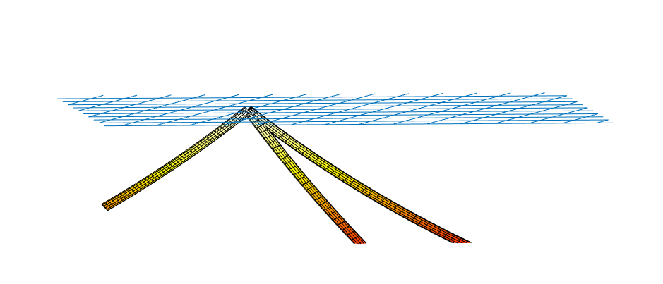
Figure 1. Schrödinger tubes

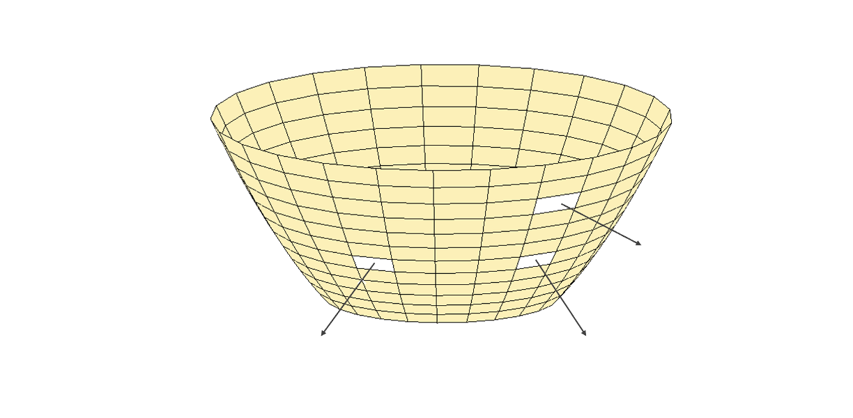
Figure 2. Euclidean case

Let us now state the properties of the kernels $K_{\nu}^{c_{0}\theta}(x,t;y,s)$ that we shall require. To simplify the statements and to also most easily apply Lee’s [23] results, let us work in Fermi normal coordinates about the geodesic $x_{j}(s)$ in (3.26) (see [16]). In these coordinates the geodesic becomes part of the last coordinate axis, i.e., $(0,\dots,0,s)$ in ${\mathbb{R}}^{n-1}$, with, as in the constructions of the symbols of the $A^{c_{0}\theta}_{\nu}$, $s$ close to the origin. For the remainder of the section, abusing notation a bit, $x=(x_{1},\dots,x_{n-1})$ denotes these Fermi normal coordinates. We then have

(3.28) $$d_{g}((0,\dots,0,x_{n-1}),(0,\dots,0,y_{n-1}))=|x_{n-1}-y_{n-1}|,$$

and, moreover, on our spatial geodesic in (3.26) we also have that the metric is simply $g_{jk}(x)=\delta^{k}_{j}$ if $x=(0,\dots,x_{n-1})$ and all the Christoffel symbols vanish there. Thus, $g_{jk}$ agrees with the standard flat rectangular metric to second order along this geodesic. See [22], [24]. Note that in these coordinates we have $(0,(0,\dots,0,1))\in\text{supp }A^{c_{0}\theta}_{j}(x,\xi)$ and so for small enough $\theta$ we have

(3.29) $$A^{c_{0}\theta}_{j}(0,\xi/|\xi|)=0\,\,\,\text{when }\,|\xi/|\xi|-(0,\dots,0,1)|\geq Cc_{0}\theta,\\ \text{and }\,\,\chi_{t}(0,(0,\dots,0,1))=(t,(0,\dots,0,1)),$$

with, as before, $\chi_{t}$ being geodesic flow, and $C$ here a uniform constant.

We can now formulate the required properties of the kernels.

Lemma 3.5.

Fix $0<\delta\ll\tfrac{1}{2}\text{Inj }M$. Assume further that $\mu=\nu,\nu^{\prime}$ are as in (3.23), and let $K_{\lambda,\mu}^{c_{0}\theta}$ be the kernel of $\tilde{\sigma}_{\lambda}A^{c_{0}\theta}_{\mu}$. In the above coordinates if $c_{0}\ll 1$ we have

(3.30) $$K_{\lambda,\mu}^{c_{0}\theta}(x,t;y,s)=\lambda^{\frac{n-1}{2}}e^{-i\lambda(d_{g}(x,y))^{2}/4(t-s)}a_{\lambda,\mu}(x,t;y,s)+O(\lambda^{-N}),\quad\mu=\nu,\nu^{\prime},$$

where, if $\nu=(c_{0}\theta j,c_{0}\theta\ell)$, and $\kappa_{\ell}^{c_{0}\theta}$ is as in (3.27),

(3.31) $$\bigl{|}\,\bigl{(}2\kappa_{\ell}^{c_{0}\theta}\tfrac{\partial}{\partial x_{n-1}}-\tfrac{\partial}{\partial t})^{m_{1}}\bigl{(}2\kappa_{\ell}^{c_{0}\theta}\tfrac{\partial}{\partial y_{n-1}}-\tfrac{\partial}{\partial s})^{m_{2}}D^{\beta}_{x,t,y,s}a_{\lambda,\mu}\bigr{|}\\ \leq C_{m_{1},m_{2},\beta}\theta^{-|\beta|},\quad\mu=\nu,\nu^{\prime}.$$

Furthermore, for small $\theta$ and $c_{0}$ there is a constant $C_{0}$ so that the above $O(\lambda^{-N})$ errors can be chosen so that the amplitudes have the following support properties: If $\overline{\gamma}_{j}$ denotes the projection onto $M^{n-1}$ of the geodesic in (2.40) and $\overline{\gamma}_{j^{\prime}}$ when $j$ is replaced by $j^{\prime}$,

(3.32) $$a_{\lambda,\mu}(x,t;y,s)=0,\quad\text{if }\,\,d_{g}(x,\overline{\gamma}_{k})+d_{g}(y,\overline{\gamma}_{k})\geq C_{1}c_{0}\theta,\\ \text{if }k=j\,\,\text{when }\nu=(c_{0}\theta j,c_{0}\theta\ell)\,\,\text{and if}\,\,k=j^{\prime}\,\,\text{when}\,\,\,\nu^{\prime}=(c_{0}\theta j^{\prime},c_{0}\theta\ell^{\prime}),$$

(3.33) $$a_{\lambda,\mu}(x,t;y,s)=0\quad\text{if }\,\,|d_{g}(x,y)+2\kappa\,(t-s)|\geq C_{0}c_{0}\theta,\\ \text{when }\,\mu=\nu\,\,\text{with}\quad\kappa=\kappa_{\ell}^{c_{0}\theta},\,\,\,\text{or }\,\,\nu=\nu^{\prime}\,\,\text{with}\quad\kappa=\kappa_{\ell^{\prime}}^{c_{0}\theta},$$

as well as

(3.34) $$a_{\lambda,\mu}(x,t;y,s)=0,\,\,\mu=\nu,\nu^{\prime},\\ \text{if }\,\,|(x_{1},\dots,x_{n-2})|+|(y_{1},\dots,y_{n-2})|+|(x_{n-1}-y_{n-1})+2\kappa^{c_{0}\theta}_{\ell}(t-s)|\geq C_{0}\theta.$$

Finally, for small $\delta_{0}>0$ in (2.6), the $O(\lambda^{-N})$ errors can be chosen so that we also have

(3.35) $$a_{\mu,\lambda}(x,t;y,s)=0\quad\text{if }\,\,\,\bigl{|}\,d_{g}(x,y)-\delta\,\bigr{|}\geq 2\delta_{0}\delta,\,\,\text{or if }\,\,x_{n-1}-y_{n-1}<0,\,\,\mu=\nu,\nu^{\prime}$$

with $\delta$ and $\delta_{0}$ as in (2.6).

This lemma is just a small variation on Lemma 4.3 in [7] (see also Lemma 3.2 in [4]), and we shall use the aforementioned result from [7] and the nature of the $\sigma_{\lambda}$ operators to obtain the above estimates. We shall postpone the proof until the final section in which we prove all the kernel estimates we have used.

Let us show now how Lemma 3.5 along with results from Lee [23] can be used to obtain Proposition 3.3.

Proof of Proposition 3.3.

To be able to prove (3.24) using Lee’s bilinear estimates we need to make one more change of variables to isolate what amounts to a “linear direction” for the phase functions in Lemma 3.5. In our earlier works on improved spectral projection estimates this was done simply by choosing Fermi normal coordinates about the spatial geodesic in (3.26). Since the kernels in Lemma 3.5 also involve a time variable, we have to deal with our time management problem by working in what amounts to “Fermi-Schrödinger” coordinates adapted to the Schrödinger tubes that we have described before. As we shall see, when we use these coordinates we use a simple parabolic scaling argument allowing us to apply the main estimate in [23]. We should also point out that the coordinate system we are about to describe is associated to the tube $\iota_{\nu}$ in (3.27) that is associated with the amplitude $a_{\lambda,\nu}$ of the kernel $K^{c_{0}\theta}_{\lambda,\nu}$ but not the amplitude other kernel $K^{c_{0}\theta}_{\lambda,\nu^{\prime}}$ in the lemma.

To describe these coordinates we first recall that, by (3.28), the last spatial coordinate $x_{n-1}$ measures distance along the spatial geodesic partially defining $\iota_{\nu}$. The “Fermi-Schrödinger” coordinates will preserve the first $(n-2)$ spatial coordinates but involve a linear change of variables in the last two coordinates $(x_{n-1},t)$ that takes into account the speeds of the spatial geodesics in (3.27), i.e., $2\kappa_{\ell}^{c_{0}\theta}$, with $\nu=(c_{0}\theta j,c_{0}\theta\ell)$ as before and $\kappa_{\ell}^{c_{0}\theta}$ as in (2.42). The “Schrödinger coordinates” that we employ are the quantum analog of the “free-fall coordinates” in relativity theory described in Manasse and Misner [24].

We note that if

(3.36) $$\varphi(x,t;y,s)=\frac{-(d_{g}(x,y))^{2}}{4(t-s)},$$

is the phase function of the kernels in (3.30), then since we are working in Fermi normal coordinates, we have along our spatial geodesic

(3.37) $$\frac{\partial}{\partial x_{j}}\varphi,\,\,\frac{\partial}{\partial y_{j}}\varphi=0\,\,\,\text{if }\,\,x=(0,\dots,0,x_{n-1}),\,\,y=(0,\dots,0,y_{n-1})\,\,\,\text{and }\,\,j=1,\dots,n-2.$$

This is not valid, though, for either of the two remaining coordinates $x_{n-1}$ or $t$ that we are currently using. We need to change coordinates so that, in the new variable, we will have the analog of (3.37) for the $(n-1)$-th variable, and, simultaneously, have that the phase function is linear in the other remaining variable when restricted to $\iota_{\nu}$.

Fortunately, this is easy to do. We simply define new variables $(\tilde{x}_{n-1},\tilde{t})$ via

(3.38) $$(x_{n-1},t)=\tilde{t}(2\kappa_{\ell}^{c_{0}\theta},-1)+\tilde{x}_{n-1}(\kappa_{\ell}^{c_{0}\theta},-1)=(2\kappa_{\ell}^{c_{0}\theta}\tilde{t}+\kappa_{\ell}^{c_{0}\theta}\tilde{x}_{n-1},-\tilde{t}-\tilde{x}_{n-1}).$$

Note then, for later use that

(3.39) $$(\tilde{x}_{n-1},\tilde{t})=-(\kappa_{\ell}^{c_{0}\theta})^{-1}\cdot\bigl{(}x_{n-1}+2\kappa_{\ell}^{c_{0}\theta}t,-x_{n-1}-\kappa_{\ell}^{c_{0}\theta}t),$$

which means that the $\tilde{x}_{n-1}$ is related to the concentration in (3.33) with $\kappa=\kappa_{\ell}^{c_{0}\theta}$. As mentioned before, we shall not change the first $(n-2)$ variables and so to be consistent with our notation, we let

(3.40) $$\tilde{x}_{j}=x_{j},\quad 1\leq j\leq n-2.$$

Note that $(\tilde{x},\tilde{t})$ is on the Schrödinger curve $\iota_{\nu}$ in (3.28) if and only if $\tilde{x}=0$. Moreover, we claim that our new coordinates fulfill the two additional goals for the behavior of the phase function $\varphi$ in (3.36) on $\iota_{\nu}$.

So, we need to check that we have the analog of (3.37) for all $j=1,\dots,n-1$, i.e.,

(3.41) $$\nabla_{\tilde{x}}\varphi,\,\,\nabla_{\tilde{y}}\varphi=0\quad\text{if }\,\,\tilde{x}=\tilde{y}=0,$$

as well as

(3.42) $$\varphi(0,\tilde{t},0,\tilde{s})=(\kappa_{\ell}^{c_{0}\theta})^{2}\cdot(\tilde{t}-\tilde{s}).$$

To verify (3.41), we note that since $\tilde{x}_{j}=x_{j}$, $1\leq j\leq n-2$, (3.37) yields $\partial\varphi/\partial x_{j}=0$ and $\partial\varphi/\partial y_{j}=0$ when $\tilde{x}=\tilde{y}=0$ and $1\leq j\leq n-2$. To see that this remains true for $j=n-1$, which gives us the remaining part of (3.41), we note that, by (3.28) and (3.38),

(3.43) $$\varphi(0,\dots,\tilde{x}_{n-1},\tilde{t},0,\dots,0,\tilde{y}_{n-1},\tilde{s})=\frac{(\kappa_{\ell}^{c_{0}\theta})^{2}}{4}\cdot\frac{(2(\tilde{t}-\tilde{s})+(\tilde{x}_{n-1}-\tilde{y}_{n-1}))^{2}}{\tilde{t}-\tilde{s}+(\tilde{x}_{n-1}-\tilde{y}_{n-1})},$$

and, consequently, by calculus, we also obtain $\partial\varphi/\partial\tilde{x}_{n-1},\,\partial\varphi/\partial\tilde{y}_{n-1}=0$ when $\tilde{x}=\tilde{y}=0$. Finally, of course (3.43) yields (3.42) as well, meaning that our goals are fulfilled.

Next, we need to make a couple of more minor modifications to prove (3.24), which, in the notation of Lemma 3.5, after a little bit of arithmetic, can be rewritten as follows:

(3.44) $$\bigl{\|}(T_{1}H_{1})(T_{2}H_{2})\bigr{\|}_{L^{q/2}_{t,x}}\lesssim_{\varepsilon}\lambda^{-\frac{2n}{q}+\varepsilon}\,\theta^{-\frac{2}{n+2}}\,\|H_{1}\|_{L^{2}_{t,x}}\|H_{2}\|_{L^{2}_{t,x}},\,\,q=\tfrac{2(n+2)}{n},$$

assuming $H_{k}(y,s)=0$, $k=1,2$, if $|s|\geq C\log\lambda$, where

(3.45) $$(T_{1}H_{1})(\tilde{x},\tilde{t})=\alpha_{m}(t)\iint e^{i\lambda\varphi(\tilde{x},\tilde{t},\tilde{y},\tilde{s})}a_{\lambda,\nu}(\tilde{x},\tilde{t};\tilde{y},\tilde{s})\,H_{1}(\tilde{y},\tilde{s})\,d\tilde{y}d\tilde{s}$$

and

(3.46) $$(T_{2}H_{2})(\tilde{x},\tilde{t})=\alpha_{m}(t)\iint e^{i\lambda\varphi(\tilde{x},\tilde{t},\tilde{y},\tilde{s})}a_{\lambda,\nu^{\prime}}(\tilde{x},\tilde{t};\tilde{y},\tilde{s})\,H_{2}(\tilde{y},\tilde{s})\,d\tilde{y}d\tilde{s}.$$

We may neglect the $O(\lambda^{-N})$ errors in Lemma 3.5 since in (3.24) we are supposing that $H_{j}(s,\cdot)=0$ if $|s|\geq C\log\lambda$.

We also of course have

(3.47) $$(T_{1}H_{1}\cdot T_{2}H_{2})(\tilde{x},\tilde{t})=\bigl{(}\alpha_{m}(t)\bigr{)}^{2}\times\\ \int e^{i\lambda(\varphi(\tilde{x},\tilde{t},\tilde{y},\tilde{s})+\varphi(\tilde{x},\tilde{t},\tilde{y}^{\prime},\tilde{s}^{\prime}))}a_{\lambda,\nu}(\tilde{x},\tilde{t},\tilde{y},\tilde{s})a_{\lambda,\nu^{\prime}}(\tilde{x},\tilde{t},\tilde{y}^{\prime},\tilde{s}^{\prime})\,H_{1}(\tilde{y},\tilde{s})\,H_{2}(\tilde{y}^{\prime},\tilde{s}^{\prime})\,d\tilde{y}d\tilde{s}d\tilde{y}^{\prime}d\tilde{s}^{\prime}.$$

Note that by (3.32), (3.34) and (3.39) we have that $a_{\lambda,\mu}(\tilde{x},\tilde{t},\tilde{y},\tilde{s})=0$, $\mu=\nu,\nu^{\prime}$ if $|(\tilde{x}_{1},\dots,\tilde{x}_{n-2})|\geq C_{1}\theta$, $|(\tilde{y}_{1},\dots,\tilde{y}_{n-2})|\geq C_{1}\theta$ or $|\tilde{x}_{n-1}-\tilde{y}_{n-1}|\geq C_{1}\theta$. As a result, in order to prove (3.44), it suffices to control the left side when the norm is taken over sets where $|\tilde{x}-(0,\dots,0,r)|\leq C_{2}\theta$, with $C_{2}$ fixed, and so, since we may take $r$ to be $0$, we have reduced matters to showing that for sufficiently small $\theta$ we have with $C_{3}\approx C_{2}$,

(3.48) $$\bigl{\|}(T_{1}H_{1})(T_{2}H_{2})\bigr{\|}_{L^{q/2}_{t,x}(\{|\tilde{x}|\leq C_{3}\theta\}\times[-1,1])}\\ \lesssim_{\varepsilon}\lambda^{-\frac{2n}{q}+\varepsilon}\,\theta^{-\frac{2}{n+2}}\,\|H_{1}\|_{L^{2}_{\tilde{t},\tilde{x}}}\|H_{2}\|_{L^{2}_{\tilde{t},\tilde{x}}},\,\,q=\tfrac{2(n+2)}{n},$$

assuming, as above, that $H_{k}(y,s)=0$, $k=1,2$, if $|s|\geq C\log\lambda$.

Next, we note that by (3.31), (3.38) and (3.39) we have that if we use the parabolic scaling $(\tilde{x},\tilde{t})\to(\theta\tilde{x},\tilde{t})$ then

(3.49) $$D^{\beta}_{\tilde{x},\tilde{t},\tilde{y},\tilde{s}}a_{\lambda,\mu}(\theta\tilde{x},\tilde{t},\theta\tilde{y},\tilde{s})=O_{\beta}(1).$$

This is clear for $\mu=\nu$ since then $2\kappa^{c_{0}\theta}_{\ell}\tfrac{\partial}{\partial x_{n-1}}-\tfrac{\partial}{\partial t}$ corresponds to $\tfrac{\partial}{\partial\tilde{t}}$, and the bounds also hold for $\mu=\nu^{\prime}$ since $\kappa_{\ell}^{c_{0}\theta}-\kappa_{\ell^{\prime}}^{c_{0}\theta}=O(\theta)$. Also note that the dilated amplitude in (3.49) is $O(\lambda^{-N})$ when $|\tilde{x}|$ or $|\tilde{y}|$ is larger than a fixed constant.

The phase function $\varphi(\tilde{x},\tilde{t},\tilde{y},\tilde{s})$ does not quite satisfy the bounds in (3.49); however, it is straightforward to remedy this if we recall that we constructed our Fermi-Schrödinger coordinates so that (3.41) and (3.42) would be valid. As a result

(3.50) $$\tilde{\varphi}(\tilde{x},\tilde{t},\tilde{y},\tilde{s})=\varphi(\tilde{x},\tilde{t},\tilde{y},\tilde{s})-\bigl{(}\kappa^{c_{0}\theta}_{\ell}\bigr{)}^{2}\,(\tilde{t}-\tilde{s})$$

vanishes to second order when $\tilde{x}=0$ and $\tilde{y}=0$. This means that, after the above parabolic scaling, we actually have

(3.51) $$D^{\beta}_{\tilde{x},\tilde{t},\tilde{y},\tilde{s}}\bigl{(}\theta^{-2}\tilde{\varphi}(\theta\tilde{x},\tilde{t},\theta\tilde{y},\tilde{s})\bigr{)}=O_{\beta}(1)\quad\text{if }\,\,|\tilde{x}|,|\tilde{y}|=O(1).$$

Clearly, in order to prove (3.48) we may replace $\varphi$ by $\tilde{\varphi}$. Also, by Minkowski’s inequality and the Schwarz inequality, if we define the “frozen” bilinear oscillatory integral operators

(3.52) $$B_{\lambda,\nu,\nu^{\prime}}^{\tilde{s},\tilde{s}^{\prime}}(h_{1},h_{2})(x,t)=(\alpha_{m}(t))^{2}\times\\ \iint e^{i\lambda(\tilde{\varphi}(\tilde{x},\tilde{t},\tilde{y},\tilde{s})+\tilde{\varphi}(\tilde{x},\tilde{t},\tilde{y}^{\prime},\tilde{s}^{\prime}))}a_{\lambda,\nu}(\tilde{x},\tilde{t},\tilde{y},\tilde{s})a_{\lambda,\nu^{\prime}}(\tilde{x},\tilde{t},\tilde{y}^{\prime},\tilde{s}^{\prime})\,h_{1}(\tilde{y})\,h_{2}(\tilde{y}^{\prime})\,d\tilde{y}d\tilde{y}^{\prime},$$

then it suffices to prove that

(3.53) $$\bigl{\|}B_{\lambda,\nu,\nu^{\prime}}^{\tilde{s},\tilde{s}^{\prime}}(h_{1},h_{2})\bigr{\|}_{L^{q/2}_{t,x}(\{|\tilde{x}|\leq C_{3}\theta\}\times[-1,1])}\\ \lesssim_{\varepsilon}\lambda^{-\frac{2n}{q}+\varepsilon}\,\theta^{-\frac{2}{n+2}}\,\|h_{1}\|_{L^{2}_{\tilde{x}}}\|h_{2}\|_{L^{2}_{\tilde{x}}},\,\,q=\tfrac{2(n+2)}{n}.$$

Note that $B_{\lambda,\nu,\nu^{\prime}}^{\tilde{s},\tilde{s}^{\prime}}(h_{1},h_{2})$ factors as the product of two oscillatory integral operators involving the $(\tilde{x},\tilde{t},\tilde{y})$ variables. The two phase functions are

(3.54) $$\phi_{\tilde{s}}(\tilde{x},\tilde{t};\tilde{y})=\tilde{\varphi}(\tilde{x},\tilde{t},\tilde{y},\tilde{s})\,\,\text{and }\,\,\phi_{\tilde{s}^{\prime}}(\tilde{x},\tilde{t};\tilde{y})=\tilde{\varphi}(\tilde{x},\tilde{t},\tilde{y},\tilde{s}^{\prime}).$$

In order to apply the bilinear results in [23] we need to collect a few facts about the support properties of the amplitudes of the bilinear oscillatory integrals in (3.52) which are straightforward consequences of Lemma 3.5.

Lemma 3.6.

Let $\delta<1/8$ as in (2.6) be given. Then we can fix $c_{0}>0$ in (3.21) so that there are constants $c_{\delta},C_{\delta}\in(0,\infty)$ so that for sufficiently small $\theta$ and $|\tilde{x}|\leq C_{0}\theta$, with $C_{0}$ fixed, we have

(3.55) $$\text{if }\,\,a_{\lambda,\nu}(\tilde{x},\tilde{t};\tilde{y},\tilde{s})\cdot a_{\lambda,\nu^{\prime}}(\tilde{x},\tilde{t};\tilde{y}^{\prime},\tilde{s}^{\prime})\neq 0,\\ \text{then }\,\,|\tilde{y}|,\,|\tilde{y}^{\prime}|\leq C_{\delta}\theta,\,\,\text{and }\,\,|\tilde{y}-\tilde{y}^{\prime}|\geq c_{\delta}\theta.$$

Additionally, if $\delta_{0}<1/8$ as in (2.6) is small enough, then for sufficiently small $\theta$ we have

(3.56) $$\text{if }\,a_{\lambda,\nu}(\tilde{x},\tilde{t};\tilde{y},\tilde{s})\neq 0\,\,\text{then }\,|\delta-2\kappa_{\ell}^{c_{0}\theta}(\tilde{t}-\tilde{s})|\leq 4\delta_{0}\delta,\\ \text{and }\,\,\text{if }\,a_{\lambda,\nu^{\prime}}(\tilde{x},\tilde{t};\tilde{y},\tilde{s}^{\prime})\neq 0\,\,\text{then }\,|\delta-2\kappa_{\ell}^{c_{0}\theta}(\tilde{t}-\tilde{s}^{\prime})|\leq 4\delta_{0}\delta,$$

Proof.

The first assertion in (3.55) about the size of $\tilde{y}$ and $\tilde{y}^{\prime}$ follows trivially from (3.34), (3.39) and (3.40). To see the assertion regarding the important separation of the $\tilde{y}$-variables, recall that $\nu,\nu^{\prime}\in c_{0}\theta\cdot\mathbb{Z}^{2n-3}$, and by (3.23), $|\nu-\nu^{\prime}|\in[\frac{1}{4}\theta,4^{n}\theta]$. Thus, if we write $\nu=(c_{0}\theta j,c_{0}\theta\ell)$ and $\nu^{\prime}=(c_{0}\theta j^{\prime},c_{0}\theta\ell^{\prime})$, we can divide into the following two cases:

(i) $|j-j^{\prime}|\geq\frac{1}{8}$. In this case, the spatial parts, $\overline{\gamma}_{j}$ and $\overline{\gamma}_{j^{\prime}}$ of the Schrödinger curves $\iota_{\nu}$ and $\iota_{\nu^{\prime}}$ have angle $\approx\theta$. By (3.32) if the product of the amplitudes in (3.55) is nonzero then we must have in our original Fermi normal coordinates that, for a fixed constant $C_{1}^{\prime}$, $x\in{\mathcal{T}}_{C_{1}^{\prime}c_{0}\theta}(\overline{\gamma}_{j})\cap{\mathcal{T}}_{C_{1}^{\prime}c_{0}\theta}(\overline{\gamma}_{j^{\prime}})$, $y\in{\mathcal{T}}_{C_{1}^{\prime}c_{0}\theta}(\overline{\gamma}_{j})$ and $y^{\prime}={\mathcal{T}}_{C_{1}^{\prime}c_{0}\theta}(\overline{\gamma}_{j^{\prime}})$. Here, of course, ${\mathcal{T}}_{r}(\overline{\gamma})$ denotes an $r$-tube about $\overline{\gamma}$ in $M^{n-1}$. By (3.35) we must also have $d_{g}(x,y),d_{g}(x,y^{\prime})\in[\delta-\delta_{0}\delta,\delta+\delta_{0}\delta]$ for our small $\delta_{0}>0$ if the product is nonzero. Since we are assuming (3.23) the two tubes of width $\approx c_{0}\theta$ intersect at angle $\approx\theta$ at $(x,t)$, which implies that in our original Fermi normal coordinates $|(y_{1},\dots,y_{n-2})-(y_{1}^{\prime},\dots,y_{n-2}^{\prime})|\approx\theta$ if the above product is nonzero and $c_{0}$ and $\theta$ are small. By (3.40), this yields the assertion in (3.55) about the separation of $\tilde{y}$ and $\tilde{y}^{\prime}$ under our assumption that $j\neq j^{\prime}$. Note that the smaller $\delta$ becomes we have to choose $c_{0}$ to be correspondingly small, but we are assuming here that $\delta$ is fixed (as we shall do later).

(ii) $|\ell-\ell^{\prime}|\geq\frac{1}{8}$. In this case we have $|\ell-\ell^{\prime}|\approx 1$. Recall that in our Fermi normal coordinates, we have

(3.57) $$d_{g}(x,y)=|x_{n-1}-y_{n-1}|,\,\,\,\frac{\partial}{\partial x_{j}}d_{g}(x,y),\,\,\frac{\partial}{\partial y_{j}}d_{g}(x,y)=0,\\ \text{if}\,\,x=(0,\dots,0,x_{n-1}),\,\,y=(0,\dots,0,y_{n-1}),\text{and }\,\,\,j=1,\dots,n-2.$$

Also we know that by (3.34)

(3.58) $$|(x_{1},\dots,x_{n-2})|+|(y_{1},\dots,y_{n-2})|\leq C_{0}\theta,\quad\text{if }\,a_{\lambda,\nu}a_{\lambda,\nu^{\prime}}\neq 0.$$

Since the function $d_{g}(x,y)$ is smooth when $d_{g}(x,y)\approx\delta$, by (3.57), (3.58) and Taylor’s expansion, we have

$$|d_{g}(x,y)-(x_{n-1}-y_{n-1})|,\,|d_{g}(x,y^{\prime})-(x_{n-1}-y_{n-1}^{\prime})|\leq C_{\delta}\theta^{2},\quad\text{if }\,a_{\lambda,\nu}a_{\lambda,\nu^{\prime}}\neq 0,$$

since by (3.35) both of the amplitudes vanish if $x_{n-1}-y_{n-1}<0$. If we let $\theta$ to be small enough, $C_{\delta}\theta^{2}$ is much smaller than $c_{0}\theta$, consequently, if $|(x_{n-1}-y_{n-1})+2\kappa_{\ell}^{c_{0}\theta}(t-s)|\geq C^{\prime}_{0}c_{0}\theta$ with $C_{0}^{\prime}$ large enough we must have that $|d_{g}(x,y)+2\kappa^{c_{0}\theta}_{\ell}(t-s)|\geq C_{0}c_{0}\theta$ with $C_{0}$ as in (3.33), which means that $a_{\nu}=0$ if $|(x_{n-1}-y_{n-1})+2\kappa_{\ell}^{c_{0}\theta}(t-s)|\geq C^{\prime}_{0}c_{0}\theta$ for this choice of $C^{\prime}_{0}$ (which is independent of $c_{0}$). We similarly have $a_{\nu^{\prime}}=0$ if $|(x_{n-1}-y^{\prime}_{n-1})+2\kappa_{\ell^{\prime}}^{c_{0}\theta}(t-s)|\geq C^{\prime}_{0}c_{0}\theta$. By (3.39) this means that for a uniform constant $C_{1}$ if $a_{\nu}\neq 0$ we must have $|\tilde{x}_{n-1}-\tilde{y}_{n-1}|\leq C_{1}c_{0}\theta$, and if $a_{\nu^{\prime}}\neq 0$ we must have $|(\tilde{x}_{n-1}-\tilde{y}_{n-1}^{\prime})-2(\kappa_{\ell}^{c_{0}\theta})^{-1}(\kappa^{c_{0}\theta}_{\ell^{\prime}}-\kappa^{c_{0}}_{\ell})(t-s)|\leq C_{1}c_{0}\theta$. Since (3.33) and (3.35) imply that $-(t-s)\sim\delta$ on the support of the amplitudes and thus $|2(\kappa_{\ell}^{c_{0}\theta})^{-1}(\kappa^{c_{0}\theta}_{\ell}-\kappa^{c_{0}\theta}_{\ell^{\prime}})(t-s)|$ must be larger than a fixed multiple of $\theta$ if $|\ell-\ell^{\prime}|\approx 1$ and $a_{\lambda,\nu}\cdot a_{\lambda,\nu^{\prime}}\neq 0$. So, in this case, if $c_{0}$ is small enough, we must have $|\tilde{y}_{n-1}-\tilde{y}_{n-1}^{\prime}|\approx\theta$ if $a_{\lambda,\nu}\cdot a_{\lambda,\nu^{\prime}}\neq 0$, which finishes the proof of the first assertion regarding the separation of $\tilde{y}$ and $\tilde{y}^{\prime}$ in (3.55) .

It remains to prove (3.56). Since we are assuming $|\tilde{x}|\leq C_{0}\theta$, it follows from the first part of (3.55) that both of the amplitudes in (3.56) will vanish if we do not have $|\tilde{y}|,\,|\tilde{y}^{\prime}|=O(\theta)$ and hence

(3.59) $$a_{\lambda,\nu}(\tilde{x},\tilde{t};\tilde{y},\tilde{s})=a_{\lambda,\nu^{\prime}}(\tilde{x},\tilde{t};\tilde{y},\tilde{s})=0\quad\text{if }\,\,\,|\tilde{x}_{n-1}-\tilde{y}_{n-1}|\geq C^{\prime}\theta,$$

for some constant $C^{\prime}$. By (3.39)

$$(\tilde{x}_{n-1}-\tilde{y}_{n-1},\tilde{t}-\tilde{s})=-(\kappa_{\ell}^{c_{0}\theta})^{-1}\bigl{(}x_{n-1}-y_{n-1}+2\kappa^{c_{0}\theta}_{\ell}(t-s),\,-(x_{n-1}-y_{n-1})-\kappa^{c_{0}\theta}_{\ell}(t-s))\bigr{)},$$

and so $(\tilde{x}_{n-1}-\tilde{y}_{n-1})+(\tilde{t}-\tilde{s})=-(t-s)$. Since $|\ell-\ell^{\prime}|\approx 1$ implies $\kappa^{c_{0}\theta}_{\ell}-\kappa^{c_{0}\theta}_{\ell^{\prime}}=O(\theta)$, by (3.33) and (3.59), we conclude that both amplitudes vanish if we do not have

$$|d_{g}(x,y)-2\kappa_{\ell}^{c_{0}\theta}(\tilde{t}-\tilde{s})|\leq C^{\prime}\theta,$$

for some uniform constant $C^{\prime}$. By the first part of (3.35) we obtain (3.56) if $\theta$ is sufficiently small. ∎

Let us now prove the bilinear oscillatory integral estimates (3.53) which will finish the proof of Proposition 3.3.

To prove (3.53), in addition to following the proof of [23, Theorem 1.3], we shall also follow related arguments of two of us [4] which proved analogous bilinear estimates in the $1+2$ dimensional setting (one lower dimension than here) using the simpler classical bilinear oscillatory integral estimates implicit in Hörmander [19]. Similar arguments were in the paper [5] by these two authors.

Just as in [23] we first perform a parabolic scaling as in (3.49) and (3.51) to be able to apply the main estimate, Theorem 1.1, in Lee [23]. So for small $\lambda^{-1/8}\leq\theta\ll 1$, we let

(3.60) $$\phi^{\theta}_{\tilde{s}}(\tilde{x},\tilde{t};\tilde{y})=\theta^{-2}\tilde{\varphi}(\theta\tilde{x},\tilde{t};\theta\tilde{y},\tilde{s}),\quad\text{and }\,\,\phi^{\theta}_{\tilde{s}^{\prime}}(\tilde{x},\tilde{t};\tilde{y}^{\prime})=\theta^{-2}\tilde{\varphi}(\theta\tilde{x},\tilde{t};\theta\tilde{y}^{\prime},\tilde{s}^{\prime}).$$

and corresponding amplitudes

(3.61) $$a^{\theta}_{\lambda,\nu}(\tilde{x},\tilde{t};\tilde{y},\tilde{s})=a_{\lambda,\nu}(\theta x,\tilde{t};\theta\tilde{y},\tilde{s})\quad\text{and }\,\,a^{\theta}_{\lambda,\nu^{\prime}}(\tilde{x},\tilde{t};\tilde{y},\tilde{s})=a_{\lambda,\nu}(\theta x,\tilde{t};\theta\tilde{y}^{\prime},\tilde{s}^{\prime}).$$

Then, as we noted before

$$D^{\beta}_{\tilde{x},\tilde{t},\tilde{y}}a^{\theta}_{\lambda,\mu}=O_{\beta}(1),\,\mu=\nu,\nu^{\prime}\quad\text{and }\,\,D^{\beta}_{\tilde{x},\tilde{t},\tilde{y}}\phi_{j}=O_{\beta}(1),\,\,\phi_{1}=\phi^{\theta}{\tilde{s}},\,\,\phi_{2}=\phi^{\theta}_{\tilde{s}^{\prime}}.$$

By (3.55) and (3.56) we also have the key separation properties for small enough $\theta$

(3.62) $$\text{if }\,\,a^{\theta}_{\lambda,\nu}(\tilde{x},\tilde{t};\tilde{y},\tilde{s})a^{\theta}_{\lambda,\nu^{\prime}}(\tilde{x},\tilde{t};\tilde{y}^{\prime},\tilde{s}^{\prime})\neq 0\\ \text{then }\,|\tilde{y}|,|\tilde{y}^{\prime}|=O(1),\,\,|\tilde{y}-\tilde{y}^{\prime}|\geq c_{\delta}\,\,\text{and }\,\,|\tilde{s}-\tilde{s}^{\prime}|\leq 8\delta_{0}\delta,$$

with $\delta$ and $\delta_{0}$ as in (2.6).

Additionally, by a simple scaling argument, our remaining task of the section, (3.53), is equivalent to the following for small enough $\theta$:

(3.63) $$\bigl{\|}B^{\theta,\tilde{s},\tilde{s}^{\prime}}_{\lambda,\nu,\nu^{\prime}}(h_{1},h_{2})\bigr{\|}_{L^{q/2}_{t,x}(\{|\tilde{x}_{0}|\leq C_{1}\}\times[-1,1])}\lesssim_{\varepsilon}\bigl{(}\lambda\theta^{2}\bigr{)}^{-\frac{2n}{q}+\varepsilon}\|h_{1}\|_{L^{2}_{x}}\|h_{2}\|_{L^{2}_{x}},\,q=\tfrac{2(n+2)}{n},$$

where we have the scaled version of (3.52), i.e.,

(3.64) $$B^{\mu,\tilde{s},\tilde{s}^{\prime}}_{\lambda,\nu,\nu^{\prime}}(h_{1},h_{2})(x,t)=(\alpha_{m}(t))^{2}\times\\ \iint e^{i(\lambda\theta^{2})[\phi^{\theta}_{\tilde{s}}(\tilde{x},\tilde{t};\tilde{y})+\phi^{\theta}_{\tilde{s}^{\prime}}(\tilde{x},\tilde{t};\tilde{y}^{\prime})]}a^{\theta}_{\lambda,\nu}(\tilde{x},\tilde{t};\tilde{y},\tilde{s})a^{\theta}_{\lambda,\nu^{\prime}}(\tilde{x},\tilde{t};\tilde{y}^{\prime},\tilde{s}^{\prime})\,h_{1}(\tilde{y})h_{2}(\tilde{y}^{\prime})\,d\tilde{y}d\tilde{y}^{\prime}.$$

To prove this, let us see how we can use our earlier observation that (3.41) and (3.50) implies that $\tilde{\varphi}$ vanishes to second order when $(\tilde{x},\tilde{y})=(0,0)$ to see that the scaled phase functions in (3.60) closely resemble Euclidean ones if $\theta$ is small which will allow us to verify the hypotheses of Lee’s bilinear oscillatory integral theorem [23, Theorem 1.3] if $\delta,\delta_{0}>0$ in (2.6) are fixed small enough.

To be more specific, let

(3.65) $$A(\tilde{t},\tilde{s})=\frac{\partial^{2}\tilde{\varphi}}{\partial\tilde{y}_{j}\partial\tilde{y}_{k}}(0,\tilde{t};0,\tilde{s}),\,\,\,B(\tilde{t},\tilde{s})=\frac{\partial^{2}\tilde{\varphi}}{\partial\tilde{x}_{j}\partial\tilde{y}_{k}}(0,\tilde{t};0,\tilde{s}),\\ \text{and }\,\,C(\tilde{t},\tilde{s})=\frac{\partial^{2}\tilde{\varphi}}{\partial\tilde{x}_{j}\partial\tilde{x}_{k}}(0,\tilde{t};0,\tilde{s}).$$

Then the Taylor expansion about $(\tilde{x},\tilde{y})=(0,0)$ of $\tilde{\varphi}$ is

(3.66) $$\tilde{\varphi}(\tilde{x},\tilde{t};\tilde{y},\tilde{s})=\tfrac{1}{2}\tilde{y}^{T}A(\tilde{t},\tilde{s})\tilde{y}+\tilde{x}^{T}B(\tilde{t},\tilde{s})\tilde{y}+\tfrac{1}{2}\tilde{x}^{T}C(\tilde{t},\tilde{s})\tilde{x}+r(\tilde{x},\tilde{t};\tilde{y},\tilde{s}),$$

where $r(\tilde{x},\tilde{t};\tilde{y},\tilde{s})$ vanishes to third order at $(\tilde{x},\tilde{y})=(0,0)$. So,

(3.67) $$D^{\beta}_{\tilde{x},\tilde{y},\tilde{t},\tilde{s}}r^{\theta}(\tilde{x},\tilde{t};\tilde{y},\tilde{s})=O(\theta),\quad\text{if }\,\,r^{\theta}(\tilde{x},\tilde{t};\tilde{y},\tilde{s})=\theta^{-2}r(\theta\tilde{x},\tilde{t};\theta\tilde{y},\tilde{s}),$$

which means that $r^{\theta}\to 0$ in the $C^{\infty}$ topology as $\theta\to 0$.

To use (3.66) we shall use parabolic scaling and the following lemma, whose proof we postpone until the end of this subsection, which says that if $\delta,\delta_{0}>0$ in (2.6) are small enough then the phase functions $\phi_{\tilde{s}}$ and $\phi_{\tilde{s}^{\prime}}$ in (3.54) satisfy the Carleson-Sjölin condition (see [29, §2.2.2] and [33]).

Lemma 3.7.

Let $A(\tilde{t},\tilde{s})$ and $B(\tilde{t},\tilde{s})$ be as in (3.65). Then if $\delta,\delta_{0}>0$ in (2.6) are small enough

(3.68) $$\det B(\tilde{t},\tilde{s})=\det\frac{\partial^{2}\tilde{\varphi}(0,\tilde{t};0,\tilde{s})}{\partial\tilde{x}_{j}\partial\tilde{y}_{k}}\neq 0,\quad\text{if }\,\,a^{\theta}_{\lambda,\nu}\cdot a^{\theta}_{\lambda,\nu^{\prime}}\neq 0.$$

Furthermore, on the support of $a^{\theta}_{\lambda,\nu}\cdot a^{\theta}_{\lambda,\nu^{\prime}}$, $-(\tfrac{\partial}{\partial\tilde{t}}A(\tilde{t},\tilde{s}))^{-1}=-(\tfrac{\partial}{\partial\tilde{t}}\tfrac{\partial^{2}\tilde{\varphi}}{\partial\tilde{y}_{j}\partial\tilde{y}_{k}}(0,\tilde{t};0,\tilde{s}))^{-1}$ is positive definite, i.e.,

(3.69) $$\xi^{t}\Bigl{(}-\frac{\partial}{\partial\tilde{t}}A(\tilde{t},\tilde{s})\Bigr{)}^{-1}\xi,\,\,\xi^{t}\Bigl{(}-\frac{\partial}{\partial\tilde{t}}A(\tilde{t},\tilde{s}^{\prime})\Bigr{)}^{-1}\xi\geq c_{\delta}|\xi|^{2},\quad\text{if }\,a^{\theta}_{\lambda,\nu}\cdot a^{\theta}_{\lambda,\nu^{\prime}}\neq 0,$$

and also

(3.70) $$\Bigl{|}\frac{\partial}{\partial\tilde{t}}A(\tilde{t},\tilde{s})\xi\Bigr{|}\geq c_{\delta}|\xi|,\,\Bigl{|}\frac{\partial}{\partial\tilde{t}}A(\tilde{t},\tilde{s}^{\prime})\xi\Bigr{|}\geq c_{\delta}|\xi|\,\,\,\text{if }\,\,a^{\theta}_{\lambda,\nu}\cdot a^{\theta}_{\lambda,\nu^{\prime}}\neq 0,$$

Let us use (3.66) and (3.67) and this lemma to see that we can obtain our remaining estimate (3.63) via Lee’s [23, Theorem 1.1]. As we shall see, it is crucial for us that $-\frac{\partial}{\partial\tilde{t}}A(\tilde{t},\tilde{s})$ is positive definite.

Note that, in addition to the $\theta$ parameter, (3.63) also involves the $(\tilde{s},\tilde{s}^{\prime})$ parameters. For simplicity, let us first see how Lee’s result yields (3.63) in the case where these two parameters agree, i.e. $\tilde{s}=\tilde{s}^{\prime}$. We then will argue that if $\delta_{0}$ in (2.6) and hence (3.55) is fixed small enough we can also handle the case where $\tilde{s}\neq\tilde{s}^{\prime}$.

To do this we first note that the parabolic scaling in (3.67), which agrees with that in (3.60), preserves the first three terms in the right of (3.66) since they are quadratic. Also, in proving (3.64), we may subtract $\tfrac{1}{2}\tilde{x}^{t}C(\tilde{t},\tilde{s})\tilde{x}$ from $\phi^{\theta}_{\tilde{s}}$ and $\tfrac{1}{2}\tilde{x}^{t}C(\tilde{t},\tilde{s}^{\prime})\tilde{x}$ from $\phi^{\theta}_{\tilde{s}^{\prime}}$ as these quadratic terms do not involve $\tilde{y}$. We point out that this trivial reduction also works if $\tilde{s}\neq\tilde{s}^{\prime}$.

Next, we note that, by (3.68) and our temporary assumption that $\tilde{s}=\tilde{s}^{\prime}$, after making a linear change of variables in $\tilde{x}$ (depending on $\tilde{t},\tilde{s}$), we may reduce to the case where $B(\tilde{t},\tilde{s})=I_{n-1}$, the $(n-1)\times(n-1)$ identity matrix. This means for the case where $\tilde{s}=\tilde{s}^{\prime}$ we have reduced matters to showing that (3.63) is valid where

(3.71) $$\phi^{\theta}_{\tilde{s}}(\tilde{x},\tilde{t};\tilde{y})=\langle\tilde{x},\tilde{y}\rangle+\frac{1}{2}\sum_{j,k=1}^{n-1}\frac{\partial^{2}\tilde{\varphi}}{\partial\tilde{y}_{j}\partial\tilde{y}_{k}}(0,\tilde{t};0,\tilde{s})\tilde{y}_{j}\tilde{y}_{k}+\tilde{r}^{\theta}(\tilde{x},\tilde{t};\tilde{y},\tilde{s})\\ =\langle\tilde{x},\tilde{y}\rangle+\tilde{y}^{t}A(\tilde{t},\tilde{s})\tilde{y}+\tilde{r}^{\theta}(\tilde{x},\tilde{t};\tilde{y},\tilde{s}),$$

with $\tilde{r}^{\theta}$ denoting $r^{\theta}$ rewritten in the new $\tilde{x}$ variables coming from $B(\tilde{t},\tilde{s})$. In view of (3.68), (3.67) remains valid for $\tilde{r}^{\theta}$. For later use, we note that if we change variables according to $\tilde{s}$ as above, then for $\tilde{s}^{\prime}$ near $\tilde{s}$ we have for

(3.72) $$B(\tilde{t},\tilde{s},\tilde{s}^{\prime})=(B(\tilde{t},\tilde{s}^{\prime}))^{t}\,((B(\tilde{t},\tilde{s})^{-1})^{t}=I_{n-1}+O(|\tilde{s}-\tilde{s}^{\prime}|),$$

(3.73) $$\phi^{\theta}_{\tilde{s}^{\prime}}(\tilde{x},\tilde{t},\tilde{y})=\langle x,B(\tilde{t},\tilde{s},\tilde{s}^{\prime})\tilde{y}\rangle+\frac{1}{2}\sum_{j,k=1}^{n-1}\frac{\partial^{2}\tilde{\varphi}}{\partial\tilde{y}_{j}\partial\tilde{y}_{k}}(0,\tilde{t};0,\tilde{s}^{\prime})\tilde{y}_{j}\tilde{y}_{k}+\tilde{r}^{\theta}(\tilde{x},\tilde{t};\tilde{y},\tilde{s})\\ =\phi^{\theta}_{\tilde{s}}(\tilde{x},\tilde{t};\tilde{y})+O(|\tilde{s}-\tilde{s}^{\prime}|).$$

We fix $\delta$ and $\delta_{0}$ in (2.6) so that the conclusions of Lemmas 3.5 and 3.7 are valid. We can also now fix also finally fix $c_{0}$ so that the results of Lemma 3.5 and Lemma 3.6 are valid. If we only had to treat the case where $\tilde{s}=\tilde{s}^{\prime}$ in (3.63) then the above choice of $\delta_{0}$ would suffice; however, as we shall momentally see, to handle the cases where $\tilde{s}\neq\tilde{s}^{\prime}$ we shall need to choose $\delta_{0}$ small enough so that we can exploit the last part of (3.62).

Let us now verify that we can apply [23, Theorem 1.3] to obtain (3.63) for sufficiently small $\theta$. This would complete the proof of Proposition 3.3. We recall that we are assuming for now that $\tilde{s}=\tilde{s}^{\prime}$ and that we have reduced to the case where $B(\tilde{t},\tilde{s})=I_{n-1}$ and $C(\tilde{t},\tilde{s})=0$ in (3.66) and so

(3.74) $$\phi^{\theta}_{\tilde{s}}(\tilde{x},\tilde{t};\tilde{y})=\langle\tilde{x},\tilde{y}\rangle+\tfrac{1}{2}\tilde{y}^{t}A(\tilde{t},\tilde{s})\tilde{y}+\tilde{r}^{\theta}(\tilde{x},\tilde{t};\tilde{y},\tilde{s}),$$

with $\tilde{r}^{\theta}$ satisfying the bounds in (3.67).

By (3.67) and (3.74) we have

(3.75) $$\frac{\partial\phi^{\theta}_{\tilde{s}}}{\partial\tilde{x}}(\tilde{x},\tilde{t};\tilde{y})=\tilde{y}+\frac{\partial\tilde{r}^{\theta}}{\partial\tilde{x}}(\tilde{x},\tilde{t};\tilde{y},\tilde{s})=\tilde{y}+\varepsilon(\theta,\tilde{x},\tilde{t},\tilde{s};\tilde{y}),$$

where $\tilde{y}\to\varepsilon(\cdot;\,\tilde{y})$ and its derivatives are $O(\theta)$. Thus, for small enough $\theta$, the inverse function also satisfies

(3.76) $$\tilde{y}\to\bigl{(}\frac{\partial\phi^{\theta}_{\tilde{s}}}{\partial\tilde{x}}(\tilde{x},\tilde{t};\,\cdot\,)\bigr{)}^{-1}(\tilde{y})=\tilde{y}+\tilde{\varepsilon}(\theta,\tilde{x},\tilde{s};\tilde{y}),$$

where

(3.77) $$D^{\beta}_{\tilde{y}}\tilde{\varepsilon}(\theta,\tilde{x},\tilde{t},\tilde{s};\tilde{y})=O_{\beta}(\theta).$$

Define, in the notation of [23],

(3.78) $$q^{\theta}_{s}(\tilde{x},\tilde{t};\tilde{y})=\tfrac{\partial}{\partial\tilde{t}}\phi^{\theta}_{s}\bigl{(}\tilde{x},\tilde{t};\bigl{(}\tfrac{\partial\phi^{\theta}_{s}}{\partial\tilde{x}}(\tilde{x},\tilde{t};\,\cdot\,)\bigr{)}^{-1}(\tilde{y})\bigr{)}\\ =\bigl{(}\tfrac{\partial}{\partial\tilde{t}}\phi^{\theta}_{s}\bigr{)}\bigl{(}\tilde{x},\tilde{t};\tilde{y}+\tilde{\varepsilon}(\theta,\tilde{x},\tilde{t},s;\tilde{y})\bigr{)},\quad s=\tilde{s},\tilde{s}^{\prime},$$

as well as

(3.79) $$\delta^{\theta}_{\tilde{s},\tilde{s}^{\prime}}(\tilde{x},\tilde{t};\tilde{y},\tilde{y}^{\prime})=\partial_{\tilde{y}}q^{\theta}_{\tilde{s}}(\tilde{x},\tilde{t};\partial_{\tilde{x}}\phi^{\theta}_{\tilde{s}}(\tilde{x},\tilde{t};\tilde{y}))-\partial_{\tilde{y}}q^{\theta}_{\tilde{s}^{\prime}}(\tilde{x},\tilde{t};\partial_{\tilde{x}}\phi^{\theta}_{\tilde{s}^{\prime}}(\tilde{x},\tilde{t};\tilde{y}^{\prime})).$$

Even though we are assuming for the moment that $\tilde{s}=\tilde{s}^{\prime}$ these two quantities will be needed for $\tilde{s}\neq\tilde{s}^{\prime}$ as well to be able to use [23, Theorem 1.1] to obtain (3.63).

Then [23, (1.4)], the conditions to ensure the bounds (3.63), are

(3.80) $$\bigl{|}\bigl{\langle}\partial^{2}_{\tilde{x}\tilde{y}}\phi^{\theta}_{\tilde{s}}(\tilde{x},\tilde{t};\tilde{y})\delta_{\tilde{s},\tilde{s}^{\prime}}^{\theta},\,\bigl{[}\,\partial^{2}_{\tilde{x},\tilde{y}}\phi^{\theta}_{\tilde{s}}(\tilde{x},\tilde{t};\tilde{y})\,\bigr{]}^{-1}\bigl{[}\,\partial^{2}_{\tilde{y}\tilde{y}}q^{\theta}_{\tilde{s}}(\tilde{x},\tilde{t};\partial_{\tilde{x}}\phi^{\theta}_{\tilde{s}}(\tilde{x},\tilde{t};\tilde{y}))\,\bigr{]}^{-1}\delta_{\tilde{s},\tilde{s}^{\prime}}^{\theta}\bigr{\rangle}\bigr{|}>0,\\ \quad\delta_{\tilde{s},\tilde{s}^{\prime}}^{\theta}=\delta^{\theta}_{\tilde{s},\tilde{s}^{\prime}}(\tilde{x},\tilde{t};\tilde{y},\tilde{y}^{\prime}),\quad\text{on }\,\,\,\text{supp }(a_{\lambda,\nu}\cdot a_{\lambda,\nu^{\prime}}),$$

as well as

(3.81) $$\bigl{|}\bigl{\langle}\partial^{2}_{\tilde{x}\tilde{y}}\phi^{\theta}_{\tilde{s}^{\prime}}(\tilde{x},\tilde{t};\tilde{y}^{\prime})\delta_{\tilde{s},\tilde{s}^{\prime}}^{\theta},\bigl{[}\partial^{2}_{\tilde{x},\tilde{y}}\phi^{\theta}_{\tilde{s}^{\prime}}(\tilde{x},\tilde{t};\tilde{y}^{\prime})\,\bigr{]}^{-1}\bigl{[}\,\partial^{2}_{\tilde{y}\tilde{y}}q^{\theta}_{\tilde{s}^{\prime}}(\tilde{x},\tilde{t};\partial_{\tilde{x}}\phi^{\theta}_{\tilde{s}^{\prime}}(\tilde{x},\tilde{t};\tilde{y}^{\prime}))\bigr{]}^{-1}\delta_{\tilde{s},\tilde{s}^{\prime}}^{\theta}\bigr{\rangle}\bigr{|}>0,\\ \quad\delta_{\tilde{s},\tilde{s}^{\prime}}^{\theta}=\delta^{\theta}_{\tilde{s},\tilde{s}^{\prime}}(\tilde{x},\tilde{t};\tilde{y},\tilde{y}^{\prime}),\quad\text{on }\,\,\,\text{supp }(a_{\lambda,\nu}\cdot a_{\lambda,\nu^{\prime}}).$$

Note that by (3.67), (3.71), (3.93), (3.77) and (3.78) for small $\theta$ we have

(3.82) $$\bigl{(}q^{\theta}_{\tilde{s}}(\tilde{x},\tilde{t};\tilde{y})\bigr{)}^{-1}=\bigl{(}\tfrac{\partial A}{\partial\tilde{t}}(\tilde{t},\tilde{s})\bigr{)}^{-1}+O(\theta),$$

and also, by (3.75) and (3.76),

(3.83) $$\partial^{2}_{\tilde{x},\tilde{y}}\phi^{\theta}_{\tilde{s}}(\tilde{x},\tilde{t};\tilde{y})=I_{n-1}+O(\theta),$$

as well as

(3.84) $$\bigl{(}\partial^{2}_{\tilde{x},\tilde{y}}\phi^{\theta}_{\tilde{s}}(\tilde{x},\tilde{t};\tilde{y})\bigr{)}^{-1}=I_{n-1}+O(\theta).$$

By (3.71), (3.70), (3.78) and the separation condition in (3.55), if $\tilde{s}=\tilde{s}^{\prime}$ we have

(3.85) $$|\delta^{\theta}_{\tilde{s},\tilde{s}}(\tilde{x},\tilde{t};\tilde{y},\tilde{y}^{\prime})|>0\quad\text{on }\,\,\text{supp }(a_{\lambda,\nu}\cdot a_{\lambda,\nu^{\prime}}),$$

if $\theta$ is small enough. Thus, in this case the quantities inside the absolute values in (3.80) and (3.81) equal

(3.86) $$\bigl{\langle}\delta^{\theta}_{\tilde{s},\tilde{s}}(\tilde{x},\tilde{t};\tilde{y},\tilde{y}^{\prime}),\,\bigl{(}\tfrac{\partial A}{\partial t}(\tilde{t},s)\bigr{)}^{-1}\delta^{\theta}_{\tilde{s},\tilde{s}}(\tilde{x},\tilde{t};\tilde{y},\tilde{y}^{\prime})\bigr{\rangle}+O(\theta)\,\,\,\text{on }\,\,\text{supp }(a_{\lambda,\nu}\cdot a_{\lambda,\nu^{\prime}}),$$

and, therefore, by (3.69) and (3.85) the conditions (3.80) and (3.81) are valid for small enough $\theta$ when $\tilde{s}=\tilde{s}^{\prime}$. So, by [23, Theorem 1.1], we obtain (3.63), we obtain (3.63) in this case.

If $\tilde{s}\neq\tilde{s}^{\prime}$ in (3.63), we must replace $\delta^{\theta}_{\tilde{s},\tilde{s}}$ by $\delta^{\theta}_{\tilde{s},\tilde{s}^{\prime}}$. In order to accommodate this, we first need to use the fact that, by the last part of (3.55),

$$\delta^{\theta}_{\tilde{s},\tilde{s}^{\prime}}(\tilde{x},\tilde{t};\tilde{y},\tilde{y}^{\prime})=\delta^{\theta}_{\tilde{s},\tilde{s}}(\tilde{x},\tilde{t};\tilde{y},\tilde{y}^{\prime})+O(|\tilde{s}-\tilde{s}^{\prime}|)\quad\text{on }\,\text{supp }(a_{\lambda,\nu}\cdot a_{\lambda,\nu^{\prime}}).$$

Thus, by the last part of (3.62),

$$\delta^{\theta}_{\tilde{s},\tilde{s}^{\prime}}(\tilde{x},\tilde{t};\tilde{y},\tilde{y}^{\prime})=\delta^{\theta}_{\tilde{s},\tilde{s}}(\tilde{x},\tilde{t};\tilde{y},\tilde{y}^{\prime})+O(\delta_{0})\quad\text{on }\,\text{supp }(a_{\lambda,\nu}\cdot a_{\lambda,\nu^{\prime}}).$$

This means that, if we replace $O(\theta)$ by $O(\theta+\delta_{0})$ in (3.86), then the quanitity in (3.80) is of this form.

The other condition, (3.81) involves the phase function $\phi^{\theta}_{\tilde{s}^{\prime}}$ and the associated $q^{\theta}_{\tilde{s}^{\prime}}$. However if $B=B(\tilde{t},\tilde{s},\tilde{s}^{\prime})$ is as in (3.72), then we have the analog of (3.75) where we replace the first term in the right side of (3.75) by $B\tilde{y}$ and the first term in the right side of (3.76) by $B^{-1}\tilde{y}$. Also, of course $\tfrac{\partial A}{\partial\tilde{t}}(\tilde{t},\tilde{s}^{\prime})=\tfrac{\partial A}{\partial\tilde{t}}(\tilde{t},\tilde{s})+O(|\tilde{s}-\tilde{s}^{\prime}|)$. Consequently, $q^{\theta}_{\tilde{s}^{\prime}}$ will agree with $q^{\theta}_{\tilde{s}}$ when $a_{\lambda,\nu}\cdot a_{\lambda,\nu^{\prime}}\neq 0$ up to a $O(|s-s^{\prime}|)=O(\delta_{0})$ error, and by (3.72) the analogs of (3.83) and (3.84) remain valid if $\tilde{s}$ is replaced by $\tilde{s}^{\prime}$ if $O(\theta)$ there is replaced by $O(\theta+\delta_{0})$. So, like (3.80), if we replace $O(\theta)$ by $O(\theta+\delta_{0})$ in (3.86), then the quantity in (3.81) is of this form.

Thus, if $\delta_{0}$ in (2.6) is (finally) fixed small enough, and, as above, $\theta$ is small enough we conclude that the condition (1.4) in [23] is valid, which yields (3.63) and completes the proof of Proposition 3.3. ∎

Proof of Lemma 3.7.

Let us first prove (3.69) and (3.70) since they are slightly more difficult than the other estimate, (3.68), in the lemma.

If we recall (3.50) we see that

(3.87) $$A(\tilde{t},\tilde{s})=\frac{\partial^{2}\tilde{\varphi}}{\partial\tilde{y}_{j}\partial\tilde{y}_{k}}(0,\tilde{t};0,\tilde{s})=\frac{\partial^{2}\varphi}{\partial\tilde{y}_{j}\partial\tilde{y}_{k}}(0,\tilde{t};0,\tilde{s}),$$

where $\varphi$ is as in (3.36).

By (3.43) we have

(3.88) $$\frac{\partial^{2}\varphi}{\partial\tilde{y}_{n-1}^{2}}(0,\tilde{t};0,\tilde{s})=\frac{(\kappa_{\ell}^{c_{0}\theta})^{2}}{2(\tilde{t}-\tilde{s})}.$$

Additionally, by (3.38) and (3.39) we have

(3.89) $$\varphi(0,\tilde{t};\tilde{y},\tilde{s})=\frac{\big{[}d_{g}\bigl{(}(0,\dots,0,2\kappa_{\ell}^{c_{0}\theta}\tilde{t}),\,(\tilde{y}_{1},\dots,\tilde{y}_{n-2},2\kappa^{c_{0}\theta}_{\ell}\tilde{s}+\kappa_{\ell}^{c_{0}\theta}\tilde{y}_{n-1})\bigr{)}\bigr{]}^{2}}{4(\tilde{t}-\tilde{s}-\tilde{y}_{n-1})}.$$

By (3.89) we have

(3.90) $$\frac{\partial^{2}\varphi}{\partial\tilde{y}_{j}\partial\tilde{y}_{n-1}}(0,\tilde{t};0,\tilde{s})\equiv 0,\quad\text{if }\,\,j=1,\dots,n-2.$$

The remaining part of the Hessian in (3.87) is

(3.91) $$\frac{\partial^{2}\tilde{\varphi}}{\partial\tilde{y}_{j}\partial\tilde{y}_{k}}(0,\tilde{t};0,\tilde{s})=\frac{\partial^{2}}{\partial\tilde{y}_{j}\partial\tilde{y}_{k}}\frac{\bigl{[}d_{g}\bigl{(}(0,\dots,0,,2\kappa_{\ell}^{c_{0}\theta}\tilde{t}),(\tilde{y}_{1},\dots,2\kappa_{\ell}^{c_{0}\theta}\tilde{s}\bigr{)}\bigr{]}^{2}}{4(\tilde{t}-\tilde{s})},\\ \text{when }\,\,\tilde{y}_{1}=\dots=\tilde{y}_{n-2}=0\,\,\,\text{and }\,\,1\leq j,k\leq n-2.$$

To compute this, we recall that the Schrödinger coordinates $(\tilde{x},\tilde{t})$ in (3.39) and (3.40) come from the Fermi normal coordinates $(x_{1},\dots,x_{n-1})$ about the spatial geodesic $\overline{\gamma}_{j}$, and that in these coordinates $\overline{\gamma_{j}}=(0,\dots,0,t)$ and on this geodesic the metric is $\delta_{j,k}$ (rectangular) and the Christoffel symbols vanish there as well

As a result, in the Fermi normal coordinates, we must have that the full Hessian of the square of the distance function satisfies

$$\frac{\partial^{2}}{\partial y_{j}\partial y_{k}}\bigl{[}d_{g}\bigl{(}(0,\dots,0,2\kappa_{\ell}^{c_{0}\theta}\tilde{t}),y\bigr{)}\bigr{]}^{2}=2I_{n-1},\quad\text{if }\,y=(0,\dots,0,2\kappa_{\ell}^{c_{0}\theta}\tilde{t}).$$

This along with (3.40) means that (3.91), the remaining piece of the Hessian in (3.87), must be of the form

$$\frac{\partial^{2}\varphi}{\partial\tilde{y}_{j}\partial\tilde{y}_{k}}=\frac{1}{2(\tilde{t}-\tilde{s})}\delta_{j,k}+O(1),\quad\text{if }\,\,1\leq j,k\leq n-2.$$

Note that since

$$(\tilde{t},\tilde{y}_{1},\dots,\tilde{y}_{n-2})\to d_{g}((0,\dots,0,2\kappa^{c_{0}\theta}_{\ell}\tilde{t}),(\tilde{y}_{1},\dots,\tilde{y}_{n-2},2\kappa^{c_{0}\theta}_{\ell}\tilde{s}^{\prime}))$$

is smooth we also obtain

(3.92) $$\frac{\partial}{\partial\tilde{t}}\frac{\partial^{2}\varphi}{\partial\tilde{y}_{j}\partial\tilde{y}_{k}}(0,\tilde{t};0,\tilde{s})=\frac{-1}{2(\tilde{t}-\tilde{s})^{2}}\delta_{j,k}+O((\tilde{t}-\tilde{s})^{-1}),\,\,1\leq j,k\leq n-2.$$

Therefore, by (3.65), (3.87), (3.88), (3.90) and (3.92), we have

(3.93) $$-2(\tilde{t}-\tilde{s})^{2}\frac{\partial}{\partial\tilde{t}}A(\tilde{t},\tilde{s})=-2(\tilde{t}-\tilde{s})^{2}\frac{\partial}{\partial\tilde{t}}\frac{\partial^{2}\tilde{\varphi}}{\partial\tilde{y}_{j}\partial\tilde{y}_{k}}(0,\tilde{t};0,\tilde{s})=J_{\kappa_{\ell}^{c_{0}\theta}}+O(|\tilde{t}-\tilde{s}|),\\ \text{if }\quad J_{\kappa_{\ell}^{c_{0}\theta}}=\text{diag }(1,\dots,1,(\kappa_{\ell}^{c_{0}\theta})^{2}).$$

Note that $\kappa^{c_{0}\theta}_{\ell}\in[1/10,10]$. Therefore by (3.56) if $\delta$ is fixed small enough in (2.6) and if $\delta_{0}$ there is smaller than $1/8$, by (3.56), we have that $-(\partial A(\tilde{t},\tilde{s})/\partial\tilde{t})^{-1}$ is positive definite on the support of the amplitudes in (3.64). Thus, we obtain (3.69) and (3.70) for some $c_{\delta}>0$. Indeed, one may take $c_{\delta}\sim\delta^{-2}$,

The proof of the other (3.68) is very similar. If we use (3.36) we see that since, by (3.35) and (3.56), $d_{g}(x,y)\approx|t-s|\approx\delta$ on $\text{supp }a^{\theta}_{\lambda,j}\cdot a^{\theta}_{\lambda,\nu^{\prime}}$, we may assume that $|x|,\,|y|\leq C\delta$. We then have

$$(d_{g}(x,y))^{2}=|x-y|^{2}+r(x,y),\quad\text{where }\,r(x,y)=O\big{(}(|x|+|y|)|x-y|^{2}\big{)}\,\,\text{and }\,r\in C^{\infty}.$$

Therefore, by (3.38), (3.50) and (3.39), if $\bar{x}=(\tilde{x}_{1},\tilde{x}_{2},\dots,\tilde{x}_{n-2})$ and $\bar{y}=(\tilde{y}_{1},\tilde{y}_{2},\dots,\tilde{y}_{n-2})$

(3.94) $$\tilde{\varphi}(\tilde{x},\tilde{t};\tilde{y},\tilde{s})=\frac{(\kappa_{\ell}^{c_{0}\theta})^{2}(\tilde{x}_{n-1}-\tilde{y}_{n-1})^{2}+|\bar{x}-\bar{y}|^{2}+r(x,y)}{4\big{(}\tilde{t}-\tilde{s}+(\tilde{x}_{n-1}-\tilde{y}_{n-1})\big{)}}-(\kappa_{\ell}^{c_{0}\theta})^{2}(\tilde{t}-\tilde{s}).$$

Consequently, by the proof of (3.69) and (3.70) we have that for $J_{\kappa_{\ell}^{c_{0}\theta}}$ as above

$$B(\tilde{t},\tilde{s})=\frac{\partial^{2}\tilde{\varphi}}{\partial\tilde{x}_{j}\partial\tilde{y}_{k}}(0,\tilde{t};0,\tilde{s})=-\frac{1}{2(\tilde{t}-\tilde{s})}J_{\kappa_{\ell}^{c_{0}\theta}}+O(1),$$

which yields (3.68) if $\delta$ is small enough. ∎

4. Kernel estimates

In this section we finish up matters by proving the various kernel estimates that we have utilized.

4.1. Basic kernel estimates on manifolds of nonpositive curvature

Let us prove the kernel estimates that we used on $A_{+}$.

Proposition 4.1.

Let $S_{\lambda}(x,t;y,s)$ denote the kernel

$$\eta(t/T)\eta(s/T)\beta^{2}(P/\lambda)\bigl{(}e^{-i(t-s)\lambda^{-1}\Delta_{g}}\bigr{)}(x,y).$$

Then if $M=M^{n-1}$ has nonpositive sectional curvatures and $T=c_{0}\log\lambda$ with $c_{0}=c_{0}(M)>0$ sufficiently small, we have for $\lambda\gg 1$

(4.1) $$|S_{\lambda}(x,t;y,s)|\leq C\lambda^{\frac{n-1}{2}}|t-s|^{-\frac{n-1}{2}}\exp(C_{M}|t-s|).$$

To prove this we note that for fixed $t$ and $s$, $\beta^{2}(P/\lambda)e^{-i(t-s)\lambda^{-1}\Delta_{g}}=\beta^{2}(P/\lambda)e^{i(t-s)\lambda^{-1}P^{2}}$ is the Fourier multiplier operator on $M^{n-1}$ with

(4.2) $$m(\lambda,t-s;\tau)=\beta^{2}(|\tau|/\lambda)e^{i(t-s)\lambda^{-1}\tau^{2}}.$$

We have extended $m$ to be an even function of $\tau$ so that we can write

(4.3) $$\beta^{2}(P/\lambda)e^{-i(t-s)\lambda^{-1}\Delta_{g}}=(2\pi)^{-1}\int_{-\infty}^{\infty}\hat{m}(\lambda,t-s;r)\,\cos r\sqrt{-\Delta_{g}}\,dr,$$

where

(4.4) $$\hat{m}(\lambda,t-s;r)=\int_{-\infty}^{\infty}e^{-i\tau r}\beta^{2}(|\tau|/\lambda)\,e^{i(t-s)\lambda^{-1}\tau^{2}}\,d\tau.$$

We note that, by a simple integration by parts argument,

(4.5) $$\partial^{k}_{r}\hat{m}(\lambda,t-s;r)=O(\lambda^{-N}(1+|r|)^{-N})\,\forall\,N,\,\,\text{if }\,|t-s|\leq 1\,\,\text{and }\,\,\,|r|\geq C_{0},$$

with $C_{0}$ sufficiently large. Similarly

(4.6) $$\partial^{k}_{r}\hat{m}(\lambda,t-s;r)=O(\lambda^{-N}(1+|r|)^{-N})\,\forall\,N,\\ \text{if }\,|t-s|\in[2^{j-1},2^{j}],\,\,\text{and }\,\,|r|\geq C_{0}2^{j},\,\,j=1,2,\dots,$$

with $C_{0}$ fixed large enough. Since $\beta(|\tau|/\lambda)=0$ if $|\tau|\notin[\lambda/4,2\lambda]$ one may take $C_{0}=100$, as we shall do.

To use this fix an even function $a\in C^{\infty}_{0}({\mathbb{R}})$ satisfying

$$a(r)=1,\,\,|r|\leq 100\quad\text{and }\,\,a(r)=0\,\,\text{if }\,\,|r|\geq 200.$$

Then by crude eigenfunction estimates and the Weyl formula, if we let

(4.7) $$\tilde{S}_{\lambda,0}(x,t;y,s)=(2\pi)^{-1}\int a(r)\hat{m}(\lambda,t-s,r)\cos rP\,dr$$

we have

(4.8) $$\tilde{S}_{\lambda,0}(x,t;y,s)-\bigl{(}\beta^{2}(P/\lambda)e^{-i(t-s)\lambda^{-1}\Delta_{g}}\bigr{)}(x,y)=O(\lambda^{-N})\,\forall\,N\quad\text{if }\,|t-s|\leq 1,$$

and if

(4.9) $$\tilde{S}_{\lambda,j}(x,t;y,s)=(2\pi)^{-1}\int a(2^{-j}r)\hat{m}(\lambda,t-s,r)\cos rP\,dr$$

we have

(4.10) $$\tilde{S}_{\lambda,j}(x,t;y,s)-\bigl{(}\beta^{2}(P/\lambda)e^{-i(t-s)\lambda^{-1}\Delta_{g}}\bigr{)}(x,y)=O(\lambda^{-N})\,\forall\,N\\ \text{if }\,|t-s|\in[2^{j-1},2^{j}],\,\,j=1,2,\dots.$$

Consequently, we would have (4.1) if we could show that

(4.11) $$|\tilde{S}_{\lambda,0}(x,t;y,s)|\leq\lambda^{\frac{n-1}{2}}|t-s|^{-\frac{n-1}{2}}\quad\text{when }\,\,|t-s|\leq 1,$$

as well as

(4.12) $$|\tilde{S}_{\lambda,j}(x,t;y,s)|\leq\lambda^{\frac{n-1}{2}}\exp(C2^{j}),\quad\text{if }\,|t-s|\in[2^{j-1},2^{j}]\\ \text{with }\,\,j=1,2,\dots\,\,\text{and }\,\,\,2^{j}\leq c_{0}\log\lambda$$

with $c_{0}=c_{0}(M)$ fixed small enough.

To prove (4.11) and (4.12) we shall argue as in Bérard [2] (see also [28, §3.6]). Just as in [2], [6], [31] and other works we shall want to use the Hadamard parametrix and the Cartan-Hadamard theorem to lift the calculations that will be needed up to the universal cover $({\mathbb{R}}^{n-1},\tilde{g})$ of $(M^{n-1},g)$.

We therefore let $\{\alpha\}=\Gamma$ denote the group of deck transfermations preserving the associated covering map $\kappa:{\mathbb{R}}^{n-1}\to M^{n-1}$ coming from the exponential map at the point in $M^{n-1}$ with coordinates $0$ in $\Omega$ in §4 above. The metric $\tilde{g}$ on ${\mathbb{R}}^{n-1}$ is the pullback of the metric $g$ on $M^{n-1}$ via $\kappa$. Choose a Dirichlet domain $D\simeq M^{n-1}$ for $M^{n-1}$ centered at the lift of the point with coordinates $0$.

As in earlier works (see [28]) we recall that if $\tilde{x}$ denotes the lift of $x\in M^{n-1}$ to $D$, then we have the following formula

(4.13) $$(\cos tP)(x,y)=(\cos t\sqrt{-\Delta_{g}})(x,y)=\sum_{\alpha\in\Gamma}\bigl{(}\cos t\sqrt{-\Delta_{\tilde{g}}}\bigr{)}(\tilde{x},\alpha(\tilde{y})).$$

As a result, if we set

(4.14) $$K_{\lambda,0}(\tilde{x},t;\tilde{y},s)=(2\pi)^{-1}\int a(r)\hat{m}(\lambda,t-s;r)\,\bigl{(}\cos r\sqrt{-\Delta_{\tilde{g}}}\bigr{)}(\tilde{x},\tilde{y})\,dr,$$

we have the formula

(4.15) $$\tilde{S}_{\lambda,0}(x,t;y,s)=\sum_{\alpha\in\Gamma}K_{\lambda,0}(\tilde{x},t;\alpha(\tilde{y}),s)).$$

Similarly, if we set

(4.16) $$K_{\lambda,j}(\tilde{x},t;\tilde{y},s)=(2\pi)^{-1}\int a(2^{-j}r)\hat{m}(\lambda,t-s;r)\,\bigl{(}\cos r\sqrt{-\Delta_{\tilde{g}}}\bigr{)}(\tilde{x},\tilde{y})\,dr,$$

we have

(4.17) $$\tilde{S}_{\lambda,j}(x,t;y,s)=\sum_{\alpha\in\Gamma}K_{\lambda,j}(\tilde{x},t;\alpha(\tilde{y}),s).$$

Also, by Huygen’s principle and the support properties of $a$, we have that

(4.18) $$K_{\lambda,0}(\tilde{x},\tilde{y})=0\quad\text{if }\,\,d_{\tilde{g}}(\tilde{x},\tilde{y})\geq C_{1},\,\,\,\text{and }\,\,K_{\lambda,j}(\tilde{x},\tilde{y})=0\,\,\text{if }\,\,d_{\tilde{g}}(\tilde{x},\tilde{y})\geq C_{1}2^{j}$$

for a uniform constant $C_{1}$. Based on this, we conclude that the number of non-zero summands in the right side of (4.15) is $O(1)$ since $\alpha(D)\cap\alpha^{\prime}(D)=\emptyset$ if $\alpha\neq\alpha^{\prime}$. Also, by simple volume estimates, the number of $\alpha\in\Gamma$ for which $d_{\tilde{g}}(D,\alpha(D))\leq\mu$ is $O(\exp(C\mu))$ for a uniform constant $C$ if $\mu=2^{j}$, $j=1,2,\dots$, and so the number of nonzero summands in the right side of (4.16) is $O(\exp(C2^{j}))$. As a result, we would obtain (4.11) if we could show that

(4.19) $$|K_{\lambda,0}(\tilde{x},t;\tilde{y},s)|\leq C\lambda^{\frac{n-1}{2}}|t-s|^{-\tfrac{n-1}{2}},\quad\text{if }\,\,|t-s|\leq 1,$$

while (4.12) would follow from the estimate

(4.20) $$|K_{\lambda,j}(\tilde{x},t;\tilde{y},s)|\leq C\lambda^{\frac{n-1}{2}}\exp(C2^{j}),\\ \text{if }\,\,|t-s|\in[2^{j-1},2^{j}],\,\,j=1,2,\dots,\,2^{j}\leq c_{0}\log\lambda,$$

with $c_{0}=c_{0}(M)$ sufficiently small.

To prove these two estimates, we can use the Hadamard parametrix for $\partial_{r}^{2}-\Delta_{\tilde{g}}$ since $({\mathbb{R}}^{n-1},\tilde{g})$ is a Riemannian manifold without conjugate points, i.e., its injectivity radius is infinite. Thus, we can use the Hadamard parametrix to write for $\tilde{x}\in D$, $\tilde{y}\in{\mathbb{R}}^{n-1}$ and $|r|\geq c_{0}>0$

(4.21) $$\bigl{(}\cos r\sqrt{-\Delta}_{\tilde{g}}\bigr{)}(\tilde{x},\tilde{y})=\sum_{\nu=0}^{N}w_{\nu}(\tilde{x},\tilde{y})W_{\nu}(r,\tilde{x},\tilde{y})+R_{N}(r,\tilde{x},\tilde{y})$$

where $w_{\nu}\in C^{\infty}({\mathbb{R}}^{n-1}\times{\mathbb{R}}^{n-1})$,

(4.22) $$W_{0}(r,\tilde{x},\tilde{y})=(2\pi)^{-(n-1)}\int_{{\mathbb{R}}^{n-1}}e^{id_{\tilde{g}}(\tilde{x},\tilde{y})\xi_{1}}\cos r|\xi|\,d\xi,$$

while for $\nu=1,2,\dots$, $W_{\nu}(t,\tilde{x},\tilde{y})$ is a finite linear combination of Fourier integrals of the form

(4.23) $$\int_{{\mathbb{R}}^{n-1}}e^{id_{\tilde{g}}(\tilde{x},\tilde{y})\xi_{1}}e^{\pm ir|\xi|}\alpha_{\nu}(|\xi|)\,d\xi,\,\,\text{with }\,\,\alpha_{\nu}(\tau)=0,\,\text{for }\,\tau\leq 1\,\,\text{and }\,\,\partial^{j}_{\tau}\alpha_{\nu}(\tau)\lesssim\tau^{-\nu-j},$$

and, if $N_{0}$ is given, then if $N$ is large enough,

(4.24) $$|\partial_{r}^{j}R_{N}(r,\tilde{x},\tilde{y})|\leq C\exp(Cr),\quad 0\leq j\leq N_{0}$$

for a fixed constant $C$. Furthermore, the leading coefficient $w_{0}(\tilde{x},\tilde{y})$ reflects the geometry of $({\mathbb{R}}^{n-1},\tilde{g})$. Specifically, in geodesic normal coordinates about $\tilde{x}$

$$w_{0}(\tilde{x},\tilde{y})=\bigl{(}\text{det }\tilde{g}_{ij}(\tilde{y})\bigr{)}^{-1/4}.$$

Thus, if in geodesic polar coordinates the volume element is given by

$$dV_{\tilde{g}}(\tilde{y})=\bigl{(}{\mathcal{A}}(r,\omega)\bigr{)}^{n-2}drd\omega,\,\,r=d_{\tilde{g}}(\tilde{x},\tilde{y}),$$

then

$$w_{0}(\tilde{x},\tilde{y})=\bigl{(}r/{\mathcal{A}}(r,\omega)\bigr{)}^{\frac{n-2}{2}}.$$

By the classical Günther comparison theorem from Riemannian geometry (see [12, §III.4])

(4.25) $$w_{0}(\tilde{x},\tilde{y})\leq 1,$$

and, moreover, for later use, ${\mathcal{A}}(r,\omega)\geq\tfrac{1}{K}\sinh(Kr)$ if all the sectional curvatures are $\leq-K^{2}<0$, and so

(4.26) $$w_{0}(\tilde{x},\tilde{y})\leq C_{K,N}\mu^{-N}\\ \text{if }\,\,d_{\tilde{g}}(\tilde{x},\tilde{y})\approx\mu\,\,\text{and }\,\,\text{all the sectional curvatures of }\,M^{n-1}\,\,\text{are}\,\,\leq-K^{2}<0.$$

The other coefficients in (4.21) are not as well behaved; however, Bérard [2] showed that if $N_{0}$ is fixed

(4.27) $$|\partial^{\beta}_{x}w_{\nu}(\tilde{x},\tilde{y})|\leq C\exp(Cr),\,\,|\beta|,\nu\leq N_{0},\quad r=d_{\tilde{g}}(\tilde{x},\tilde{y}),$$

for some uniform constant $C$ (depending on $\tilde{g}$ and $N_{0}$).

The facts that we have just recited are well known. One can see, for instance, [2] or [28, §1.1, §3.6] for background regarding the Hadamard parametrix, and [31] for a discussion of properties of $w_{0}$.

Let us next use the Hadamard parametrix to prove (4.19). By (4.21), it suffices to see that if we replace $(\cos r\sqrt{-\Delta_{\tilde{g}}})(\tilde{x},\tilde{y})$ in (4.14) by each of the terms in the right side of (4.21) then each such expression will satisfy the bounds in (4.19).

Let us start with the contribution of the main term in the Hadamard parametrix which is the $\nu=0$ term in (4.21). In view of (4.22) and (4.25) it would give rise to these bounds if

(4.28) $$(2\pi)^{-n}\int_{-\infty}^{\infty}\int_{{\mathbb{R}}^{n-1}}e^{id_{\tilde{g}}(\tilde{x},\tilde{y})\xi_{1}}\cos(r|\xi|)\,a(r)\,\hat{m}(\lambda,t-s;r)\,drd\xi\\ =O(\lambda^{\frac{n-1}{2}}|t-s|^{-\frac{n-1}{2}})\quad\text{when }\,\,\,|t-s|\leq 1.$$

However, by (4.2) and (4.5) and the support properties of $a$, if $|t-s|\leq 1$

(4.29) $$(2\pi)^{-1} \int_{-\infty}^{\infty}\int_{{\mathbb{R}}^{n-1}}e^{id_{\tilde{g}}(\tilde{x},\tilde{y})\xi_{1}}\cos(r|\xi|)\,a(r)\,\hat{m}(\lambda,t-s;r)\,drd\xi$$

$$=(2\pi)^{-1}\int_{-\infty}^{\infty}\int_{{\mathbb{R}}^{n-1}}e^{id_{\tilde{g}}(\tilde{x},\tilde{y})\xi_{1}}\cos(r|\xi|)\hat{m}(\lambda,t-s;r)\,drd\xi+O(\lambda^{-N})$$

$$=\int_{{\mathbb{R}}^{n-1}}e^{id_{\tilde{g}}(\tilde{x},\tilde{y})\xi_{1}}\beta^{2}(|\xi|/\lambda)e^{i(t-s)\lambda^{-1}|\xi|^{2}}\,d\xi+O(\lambda^{-N}).$$

A simple stationary phase argument shows that the last integral is $O(\lambda^{\frac{n-1}{2}}|t-s|^{-\frac{n-1}{2}})$, and so we conclude that the main term in the Hadamard parametrix leads to the desired bounds.

To estimate the contributions of the higher order terms $\nu=1,2,\dots$, we note that by the first part of (4.18) we may assume that $d_{\tilde{g}}(\tilde{x},\tilde{y})$ is bounded. So, by (4.23) the higher order terms would lead to the desired bounds since

(4.30) $$(2\pi)^{-1}\iint e^{id_{\tilde{g}}(\tilde{x},\tilde{y})\xi_{1}}e^{\pm ir|\xi|}\alpha_{\nu}(|\xi|)\,a(r)\hat{m}(\lambda,t-s;r)\,drd\xi\\ =\int_{{\mathbb{R}}^{n-1}}e^{id_{\tilde{g}}(\tilde{x},\tilde{y})\xi_{1}}\beta^{2}(|\xi|/\lambda)e^{i(t-s)\lambda^{-1}|\xi|^{2}}\,\alpha_{\nu}(|\xi|)\,d\xi+O(\lambda^{-N}),\,\,\text{if }\,\,|t-s|\leq 1,$$

and, by (4.23), together with a stationary phase argument, the last integral is $O(\lambda^{\frac{n-1}{2}-\nu}|t-s|^{-\frac{n-1}{2}})$.

We also need to see that the remainder term in (4.21) leads to the bounds

(4.31) $$\int^{\infty}_{-\infty}a(r)\hat{m}(\lambda,t-s;r)R(r,\tilde{x},\tilde{y})\,dr\\ =\int^{\infty}_{-\infty}\beta^{2}(|\tau|/\lambda)e^{i(t-s)\lambda^{-1}\tau^{2}}\,\bigl{[}a(\,\cdot\,)R(\,\cdot\,,\tilde{x},\tilde{y})\bigr{]}\,\widehat{}\,\,(\tau)\,d\tau=O(\lambda^{\frac{n-1}{2}}),\,\,\text{if }\,\,d_{\tilde{g}}(\tilde{x},\tilde{y})=O(1).$$

By (4.24), the last factor in the integral in the right, which is the Fourier transform of $r\to a(r)R(r,\tilde{x},\tilde{y})$, is $O(1)$ if $d_{\tilde{g}}(\tilde{x},\tilde{y})=O(1)$. So, by the support properties of $\beta$, the last integral in (4.31) is $O(\lambda)=O(\lambda^{\frac{n-1}{2}})$, as desired, since $n\geq 3$.

Since each term in the Hadamard parametrix has the desired contribution, the proof of (4.19) is complete.

Similar arguments will yield (4.20). We need to see that if we replace $(\cos r\sqrt{-\Delta_{\tilde{g}}})(\tilde{x},\tilde{y})$ in (4.16) by each of the terms in the right side of (4.21), then each will satisfy the bounds in (4.20) if $d_{\tilde{g}}(\tilde{x},\tilde{y})\leq C2^{j}$ and $|t-s|\in[2^{j-1},2^{j}]$ with $j=1,2,\dots$ and $2^{j}\leq c_{0}\log\lambda$ as above.

By (4.6) and (4.25) and the above argument, the $\nu=0$ term in the Hadamard parametrix will lead to a contribution of

$$(2\pi)^{-(n-1)}\int_{{\mathbb{R}}^{n-1}}e^{id_{\tilde{g}}(\tilde{x},\tilde{y})\xi_{1}}e^{i(t-s)\lambda^{-1}|\xi|^{2}}\beta^{2}(|\xi|/\lambda)\,d\xi+O(\lambda^{-N})=O(\lambda^{\frac{n-1}{2}}),$$

by stationary phase and the fact that we are assuming $|t-s|\geq 1$. By (4.27) and the above arguments each of the $\nu=1,2,\dots$ terms will have contributions which are $O(\lambda^{\frac{n-1}{2}-\nu}\cdot\exp(C2^{j}))=O(\lambda^{\frac{n-1}{2}})$ if $2^{j}\leq c_{0}\log\lambda$ with $c_{0}>0$ small enough. If we repeat the argument above for the contribution of the remainder term, we see that the contributions here will be of the form

$$\int^{\infty}_{-\infty}\beta^{2}(|\tau|/\lambda)e^{i(t-s)\lambda^{-1}\tau^{2}}\bigl{[}a(2^{-j}\,\cdot\,)R(\,\cdot\,,\tilde{x},\tilde{y})\bigr{]}\,\widehat{}\,\,(\tau)\,d\tau,$$

which, by (4.24) and the support properties of $a$, is $O(\lambda\exp(C2^{j}))=O(\lambda^{\frac{n-1}{2}}\exp(C2^{j}))$, as desired.

Since each term in the Hadamard parametrix has the desired contribution, the proof of (4.20) is complete, which finishes the proof of Proposition 4.1.

We should point out that the small $|t-s|$ estimates are universally true as in [11].

4.2. Estimates for kernels of microlocalized operators

Let us prove the kernel estimates, (2.69) and (2.70), that we used in the proof of $L^{q_{c}}(A_{-})$-estimates.

Proposition 4.2.

For each $m\in{\mathbb{Z}}$ pick $\nu(m)\in{\mathbb{Z}}^{2n-3}$ as in (2.46) and let

(4.32) $$K_{\lambda}(x,t,m;y,s,m^{\prime})=\\ \alpha_{m}(t)\alpha_{m^{\prime}}(s)\Bigl{(}A_{\nu(m)}^{\theta_{0}}\circ\bigl{(}\,\beta^{2}(P/\lambda)e^{-i\lambda^{-1}(t-s)\Delta_{g}}\,\bigr{)}\circ(A^{\theta_{0}}_{\nu(m^{\prime})})^{*}\Bigr{)}(x,y).$$

Then if $M=M^{n-1}$ has nonpositive curvature

(4.33) $$|K_{\lambda}(x,t,m;y,s,m^{\prime})|\leq C\lambda^{\frac{n-1}{2}}\,|t-s|^{-\frac{n-1}{2}},$$

provided that $|t-s|\leq c_{0}\log\lambda$ with $c_{0}=c_{0}(M)>0$ sufficiently small. Moreover, for such $|t-s|$ we have

(4.34) $$|K_{\lambda}(x,t,m;y,s,m^{\prime})|\leq C\lambda^{\frac{n-1}{2}}\,|t-s|^{-N}\,\,\forall\,N,\\ \text{if }\,|t-s|\geq 1\,\,\text{and all the sectional curvatures of }\,M^{n-1}\,\text{are negative}.$$

The uniform constants $C=C(M^{n-1})$ do not depend on the particular choice of the $\nu(m)$.

Proof.

Since, as we mentioned before, the kernels of the $A_{\nu}^{\theta_{0}}$ operators satisfy the uniform bounds

(4.35) $$\int|A_{\nu}^{\theta_{0}}(x,y)|\,dx,\,\,\,\int|A_{\nu}^{\theta_{0}}(x,y)|\,dy\,\leq C,$$

by Proposition 4.1, we obtain the above bounds when $|t-s|\leq 1$.

Also, by (4.35), if we let

(4.36) $$\tilde{K}_{\lambda}(x,t,m;y,s,m^{\prime})=\\ \alpha_{m}(t)\alpha_{m^{\prime}}(s)\Bigl{(}A_{\nu}^{\theta_{0}}\circ\bigl{(}\,\beta^{2}(P/\lambda)e^{-i\lambda^{-1}(t-s)\Delta_{g}}\,\bigr{)}\Bigr{)}(x,y),\quad\nu=\nu(m),$$

it suffices to see that this kernel, which does not include the microlocal cutoffs in the right satisfies the bounds in (4.33) and (4.34) when $|t-s|\geq 1$.

Let us start by proving that (4.36) satisfies the bounds in (4.34) for $|t-s|\geq 1$ if $M^{n-1}$ has nonpositive curvatures.

To do this recall that, by (2.42) and (2.46) with $\theta=\theta_{0}=\lambda^{-1/8}$ , if $\nu(m)=(\theta_{0}k,\theta_{0}\ell)$ then

(4.37) $$A_{\nu}^{\theta_{0}}(x,D)=\tilde{A}_{k}^{\theta_{0}}(x,D)\circ b(\lambda^{-7/8}(P-\lambda\kappa_{\ell}^{\theta_{0}})),\quad\kappa^{\theta_{0}}_{\ell}=1+\theta_{0}\ell,\,\,|\ell|\lesssim\theta_{0}^{-1},\\ \text{if }\,\,\tilde{A}_{k}^{\theta_{0}}(x,D)=A_{k}^{\theta_{0}}(x,D)\circ\tilde{\Upsilon}(P/\lambda),$$

with $b\in C^{\infty}_{0}((-1,1))$ and $\Upsilon$ as in (2.43). Here the $A_{k}^{\theta_{0}}$ operators localize at scale $\theta_{0}=\lambda^{-1/8}$ about a geodesic $\overline{\gamma}_{k}$ in $\Omega$ due to (2.37)–(2.41).

By (4.37) we now have the following variant of (4.3)

(4.38) $$A_{\nu}^{\theta_{0}}\circ\bigl{(}\beta^{2}(P/\lambda)e^{-i(t-s)\lambda^{-1}\Delta_{g}}\bigr{)} =\tilde{A}_{k}^{\theta_{0}}\circ\bigl{(}\beta^{2}(P/\lambda)\,b(\lambda^{-7/8}(P-\lambda\kappa^{\theta_{0}}_{\ell}))\,e^{-i(t-s)\lambda^{-1}\Delta_{g}}\bigr{)}$$

$$=\Bigl{(}\,(2\pi)^{-1}\int\hat{m}_{\ell}(\lambda,t-s;r)\,\bigl{(}\tilde{A}_{k}^{\theta_{0}}\circ\cos r\sqrt{-\Delta_{g}}\bigr{)}\,dr\Bigr{)},$$

if now (4.4) is replaced by

(4.39) $$\hat{m}_{\ell}(\lambda,t-s;r)=\int_{-\infty}^{\infty}e^{-i\tau r}\beta^{2}(|\tau|/\lambda)\,b(\lambda^{-7/8}(|\tau|-\lambda\kappa_{\ell}^{\theta_{0}}))e^{i(t-s)\lambda^{-1}\tau^{2}}\,d\tau.$$

By a simple integration by parts argument we have the following analog of (4.6)

(4.40) $$\partial_{r}^{k}\hat{m}_{\ell}(\lambda,t-s;r)=O(\lambda^{-N}(1+|r|)^{-N})\,\,\forall\,N\\ \text{if }\,\,|t-s|\leq c_{0}\log\lambda\,\,\,\text{and }\,\,|r|\geq 100c_{0}\log\lambda.$$

Thus, if $a$ is as in the proof of Proposition 4.1, since the dyadic operators $\tilde{A}_{k}^{\theta_{0}}$ have kernels as in (4.35), if we insert a factor of $(1-a(r/c_{0}\log\lambda))$ into the integral in the last term in (4.38) the resulting kernels will be $O(\lambda^{-N})$ for all $N$. So, we have reduced the proof of (4.33) to showing that we have the kernel estimates

(4.41) $$\bigl{(}W_{\lambda,\ell,t-s}\bigr{)}(x,y)=O(\lambda^{\frac{n-1}{2}}|t-s|^{-\frac{n-1}{2}}),\quad\text{if }\,\,1\leq|t-s|\leq c_{0}\log\lambda,$$

for small enough $c_{0}>0$ if

(4.42) $$W_{\lambda,\ell,t-s}=(2\pi)^{-1}\int a(r/c_{0}\log\lambda)\,\hat{m}_{\ell}(\lambda,t-s;r)\,\bigl{(}\tilde{A}_{k}^{\theta_{0}}\cos r\sqrt{-\Delta_{g}}\bigr{)}\,dr.$$

To estimate (4.41), we shall argue as in the last subsection. We first lift the calculation up to the universal cover exactly as before by rewriting

(4.43) $$W_{\lambda,\ell,t-s}(x,y)=\sum_{\alpha\in\Gamma}W^{\alpha}_{\lambda,\ell,t-s}(\tilde{x},\tilde{y}),$$

where

(4.44) $$W^{\alpha}_{\lambda,\ell,t-s}(\tilde{x},\tilde{y})=\\ (2\pi)^{-1}\int_{-\infty}^{\infty}a(r/c_{0}\log\lambda)\,\hat{m}_{\ell}(\lambda,t-s;r)\,\bigl{(}\tilde{A}_{k}^{\theta_{0}}\cos r\sqrt{-\Delta_{\tilde{g}}}\bigr{)}(\tilde{x},\alpha(\tilde{y}))\,dr,$$

and $\tilde{x}$, $\tilde{y}$ denote the lift of $x,y$, respectively, to the universal cover $({\mathbb{R}}^{n-1},\tilde{g})$. By the support properties of $a$ and Huygens principle

(4.45) $$W^{\alpha}_{\lambda,\ell,t-s}(\tilde{x},\alpha(\tilde{y}))=0\quad\text{if }\,\,d_{\tilde{g}}(\tilde{x},\tilde{\alpha}(\tilde{y}))\geq Cc_{0}\log\lambda,$$

with $C$ being a fixed constant.

In the last subsection we had to deal with the fact that the sums that arose after lifting the calculations up to the universal cover involved $O(\exp(Cc_{0}\log\lambda))$ terms. Here, because of the $\nu=(k,\ell)$ localizations, it will turn out that, given $|t-s|\geq 1$, there are only $O(1)$ summands above which are nontrivial.

Let us start by exploiting the localization coming from the $\tilde{A}_{k}^{\theta_{0}}$ operators which localize about the geodesic $\overline{\gamma}_{k}$ in $\Omega$. If we argue exactly in [6], just by using this operator and elementary arguments involving the calculus of Fourier integral operators and Toponogov’s triangle comparison theorem, we shall be able to see that the overwhelming majority of the terms in (4.43) are $O(\lambda^{-1/2})$, which is much better than the bounds posited above.

To do this, just as in earlier works we start by modifying the coordinates in $\Omega$ so that the $0\in\overline{\gamma}_{k}$. Then, as in [6], we let $\tilde{\gamma}(t)$, $t\in{\mathbb{R}}$ denote the lift of the geodesic $\overline{\gamma}_{k}$ to the universal cover and

$${\mathcal{T}}_{R}(\tilde{\gamma})=\{x:\,d_{\tilde{g}}(\tilde{\gamma},\tilde{z})\leq R\}.$$

Then, just as in [6], if $R$ is fixed large enough and $\alpha(D)\cap{\mathcal{T}}_{R}(\tilde{\gamma})=\emptyset$, with, as before, $D\simeq M^{n-1}$ being our fundamental domain, then the summand in (4.43) involving $\alpha$ must by $O(\lambda^{-1})$ by Toponogov’s theorem and microlocal arguments. This is exactly how (3.9) in [6] was proved, and one can simply repeat the arguments there to obtain this bound.

Since there are $O(\lambda^{1/2})$ non-zero terms in (4.43) if $c_{0}$ in (4.44) is fixed small enough, we obtain in this case

$$\sum_{\{\alpha:\,\alpha(D)\cap{\mathcal{T}}_{R}(\tilde{\gamma})=\emptyset\}}W_{\lambda,\ell,t-s}^{\alpha}(\tilde{x},\tilde{y})=O(\lambda^{-1/2}),\quad\text{if }\,1\leq|t-s|\leq c_{0}\log\lambda,$$

which is much better than the bounds in (4.41).

In order to obtain (4.41) we still have to deal with the terms for which $\alpha(D)\cap{\mathcal{T}}_{R}(\tilde{\gamma})\neq\emptyset$; however, fortunately for us, by (4.45) there are only $O(\log|t-s|)$ such non-zero terms in (4.43). Having reduced out task to only considering such summands we no longer need to use the microlocal cutoff $\tilde{A}_{k}^{\theta_{0}}$. Since it satisfies the bounds in (4.35) we would have (4.41) if

(4.46) $$\sum_{\{\alpha:\,\alpha(D)\cap{\mathcal{T}}_{R}(\tilde{\gamma})\neq\emptyset\}}(2\pi)^{-1}\int_{-\infty}^{\infty}a(r/c_{0}\log\lambda)\,\hat{m}_{\ell}(\lambda,t-s;r)\,\bigl{(}\cos r\sqrt{-\Delta_{\tilde{g}}}\bigr{)}(\tilde{x},\alpha(\tilde{y}))\,dr\\ =O(\lambda^{\frac{n-1}{2}}|t-s|^{-\frac{n-1}{2}}),\quad\text{if }\,\,1\leq|t-s|\leq c_{0}\log\lambda.$$

To do this, just like before, we shall use the Hadamard parametrix (4.21). We need to see that the contribution of each term gives a contribution satisfying the these bounds.

If we argue as before, and use (4.23) the contribution of the higher order terms to (4.44) will be a linear combination of terms of the form

(4.47) $$(2\pi)^{-1}w_{\nu}(\tilde{x},\alpha(\tilde{y}))\int_{-\infty}^{\infty}\int e^{id_{\tilde{g}}(\tilde{x},\alpha(\tilde{y}))\xi_{1}}e^{\pm ir|\xi|}\alpha_{\nu}(|\xi|)a(r/c_{0}\log\lambda)\\ \times\hat{m}_{\ell}(\lambda,t-s;r)\,d\xi dr.$$

Assuming as we are that $|t-s|\leq c_{0}\log\lambda$, modulo a $O(\lambda^{-N})$ term, just as in (4.30), this equals

(4.48) $$w_{\nu}(\tilde{x},\alpha(\tilde{y}))\int_{{\mathbb{R}}^{n-1}}\beta^{2}(|\xi|/\lambda)b(\lambda^{-7/8}(|\xi|-\lambda\kappa^{\theta_{0}}_{\ell}))\,e^{id_{\tilde{g}}(\tilde{x},\alpha(\tilde{y}))\xi_{1}}\,\alpha_{\nu}(|\xi|)\,e^{i(t-s)\lambda^{-1}|\xi|^{2}}\,d\xi.$$

By an easy stationary phase calculation if $|t-s|\geq 1$ the last integral is $O(\lambda^{\frac{n-1}{2}-\nu})$ in view of the last part of (4.23). Since, as we noted before there are only $O(\log\lambda)$ summands in (4.46), we conclude that the contribution of the higher order terms, $\nu=1,2,\dots$, in Hadamard parametrix will be $O(\lambda^{\frac{n-1}{2}-\frac{1}{2}})$, which is much better than we need for (4.46).

We next notice that, similar to (4.31), the contribution of the remainder term in (4.21) will be

$$\int_{-\infty}^{\infty}\beta^{2}(|\tau|/\lambda)e^{i(t-s)\lambda^{-1}\tau^{2}}b(\lambda^{-7/8}(|\tau|-\lambda\kappa^{\theta_{0}}_{\ell}))\bigl{[}a((c_{0}\log\lambda)^{-1}\,\cdot\,)R(\,\cdot\,,\tilde{x},\tilde{y})\bigr{]}\,\widehat{}\,\,(\tau)\,d\tau.$$

By (4.24), the last factor in the integral is $O(\exp(Cc_{0}\log\lambda))\leq\lambda^{1/16}$ if $c_{0}$ is small enough. Since the rest of the integrand is bounded and supported on a set of size $\lambda^{7/8}$, we conclude that the contribution of the remainder term in the Hadamard parametrix to (4.41) also not only satisfies the bounds in (4.46), but, moreover, like the above terms for $\nu=1,2,\dots$ in (4.21), satisfies the improved ones in (4.34). Indeed, its contribution will be $O(\lambda^{15/16}\log\lambda)$ for such $c_{0}$.

We still have to deal with the main term in the Hadamard parametrix, i.e., the contribution of the $\nu=0$ term in (4.21) to (4.47). Arguing as before, the proof of (4.46) would be complete if we could show that

(4.49) $$\sum_{\{\alpha:\,\alpha(D)\cap{\mathcal{T}}_{R}(\tilde{\gamma})\neq\emptyset\}}w_{0}(\tilde{x},\alpha(\tilde{y}))\int_{{\mathbb{R}}^{n-1}}\beta^{2}(|\xi|/\lambda)\,b(\lambda^{-7/8}(|\xi|-\lambda\kappa^{\theta_{0}}_{\ell}))\\ \times\cos(r|\xi|)e^{id_{\tilde{g}}(\tilde{x},\alpha(\tilde{y})\xi_{1}}e^{i(t-s)\lambda^{-1}|\xi|^{2}}\,dr\\ =O(\lambda^{\frac{n-1}{2}}|t-s|^{-\frac{n-1}{2}}),\quad\text{if }\,\,1\leq|t-s|\leq c_{0}\log\lambda.$$

To obtain (4.49) we shall use the fact that for $|t-s|\geq 1$ we have:

(4.50) $$\int_{{\mathbb{R}}^{n-1}}\beta^{2}(|\xi|/\lambda)b(\lambda^{-7/8}(|\xi|-\lambda\kappa))e^{id_{\tilde{g}}(\tilde{x},\alpha(\tilde{y}))\xi_{1}}e^{i(t-s)\lambda^{-1}|\xi|^{2}}\,d\xi=O(\lambda^{-N})\,\forall N\\ \text{if }\,\,d_{\tilde{g}}(\tilde{x},\alpha(\tilde{y}))\notin I_{t,s,\kappa}=\bigl{[}2|t-s|(\kappa-C\lambda^{-1/8}),\,2|t-s|(\kappa+C\lambda^{-1/8})\big{]},\,\,\text{if }\,\kappa=\kappa^{\theta_{0}}_{\ell}$$

with $C$ large enough, and

(4.51) $$\int_{{\mathbb{R}}^{n-1}}\beta^{2}(|\xi|/\lambda)b(\lambda^{-7/8}(|\xi|-\lambda\kappa))e^{id_{\tilde{g}}(\tilde{x},\alpha(\tilde{y}))\xi_{1}}e^{i(t-s)\lambda^{-1}|\xi|^{2}}\,d\xi=O(\lambda^{\frac{n-1}{2}}|t-s|^{-\frac{n-1}{2}}),\\ \text{if }\,\,d_{\tilde{g}}(\tilde{x},\alpha(\tilde{y}))\in I_{t,s,\kappa},\,\,\,\kappa=\kappa^{\theta_{0}}_{\ell}.$$

The first estimate just follows from a simple integration by parts argument. For if $\phi=d_{\tilde{g}}(\tilde{x},\tilde{y})\xi_{1}+(t-s)\lambda^{-1}|\xi|^{2}$, then, if $C$ in the definition of $I_{t,s,\kappa}$ is fixed large enough, $|\nabla_{\xi}\phi|\geq\lambda^{-1/8}$ if $d_{\tilde{g}}(\tilde{x},\tilde{y})\notin I_{\kappa,t,s}$, and, also, derivatives of the amplitude of the integral are $O(\lambda^{-7/8})$. Thus, in this case, every integration by parts gains a power of $\lambda^{-3/4}$, resulting in (4.50). The other estimate, (4.51) just follows from stationary phase.

If we note that the interval $I_{t,s,\kappa}$ has length $O(|t-s|\,\lambda^{-1/8})$ which is much smaller than 1, if as above we assume that $|t-s|\leq c_{0}\log\lambda$, we conclude that there can only be $O(1)$ terms in (4.49) which are not $O(\lambda^{-N})$, which leads to (4.49) since, by (4.25) $w_{0}$, is bounded.

This completes the proof of (4.33).

To prove the much stronger bounds (4.34) which require that $M^{n-1}$ have negative sectional curvatures, we note that the contribution of all of the terms in the Hadamard parametrix other than the main one, corresponding to $\nu=0$, involved a $\lambda$-power improvement of what was needed for (4.33) and thus lead to bounds of the form (4.34) since we are assuming that $|t-s|=O(\log\lambda)$. Thus, to prove (4.34), it is enough to show that under these curvature assumptions we have the analog of (4.49) with $O(\lambda^{\frac{n-1}{2}}|t-s|^{-\frac{n-1}{2}})$ replaced by $O(\lambda^{\frac{n-1}{2}}|t-s|^{-N})$ for every $N$. To do this, we also use the simple fact, which follows from an integration by parts argument, that we have the $O(\lambda^{-N})$ bounds in (4.50) if $d_{\tilde{g}}(\tilde{x},\alpha(\tilde{y}))\notin[C_{1}^{-1}|t-s|,C_{1}|t-s|]$ with $C_{1}$ fixed sufficiently large. In view of (4.26) each of the $O(1)$ nontrivial terms in the sum in the left side of (4.49) must be $O(\lambda^{\frac{n-1}{2}}|t-s|^{-N})$ for every $N$, as desired. This completes the proof of Proposition 4.2. ∎

4.3. Estimates for kernels involving local auxiliary operators.

Let us prove the kernel estimates we used in §3.

Proof of Lemma 3.5. Let us now prove Lemma 3.5, which allowed us to use parabolic scaling and results from [23] to obtain the bilinear estimates (3.63). This lemma follows from a straightforward variation on the stationary phase arguments used to prove [29, Lemma 5.1.2]. Moreover, Lemma 3.5 is essentially Lemma 3.2 in [5] or Lemma 4.3 in [7], and in fact the latter result almost immediately gives our results given how we have constructed the local operators in (2.5).

We first note that the kernel of our local operators are given by

(4.52) $$\tilde{\sigma}_{\lambda}(x,t;y,s)=\bigl{(}B\circ\sigma_{\lambda}\bigr{)}(x,t;y,s)\\ =(2\pi)^{-2}\iint e^{i(t-s)\tau}e^{ir\lambda^{1/2}\tau^{1/2}}\tilde{\beta}(\tau/\lambda)\,\hat{\sigma}(r)\,\bigl{(}B\circ e^{-irP}\bigr{)}(x,y)\,drd\tau.$$

Since $(r,x,y)\to(B\circ e^{-irP})(x,y)$ is smooth when $d_{g}(x,y)\neq|r|$ and $\hat{\sigma}$ is as in (2.6), by a simple integration by parts argument,

(4.53) $$\tilde{\sigma}_{\lambda}(x,t;y,s)=O(\lambda^{-N})\,\forall\,N\quad\text{if }\,\,|d_{g}(x,y)-\delta|\geq\tfrac{3}{2}\delta_{0}\delta.$$

This leads to the first part of (3.35) if $\theta$ is small since the kernels of our microlocal cutoffs, $A_{\nu}^{c_{0}\theta}$, satisfy

(4.54) $$A^{c_{0}\theta}_{\nu}(x,y)=O(\lambda^{-N})\,\forall\,N\quad\text{if }\,\,d_{g}(x,y)\geq C_{1}\theta,$$

for a uniform constant $C_{1}$ since we are assuming that $\lambda^{-1/2}\ll\lambda^{-1/8}\leq\theta$. Also, since the symbols $A_{\nu}^{c_{0}\theta}(x,\xi)=0$ if $\xi$ is not in a small conic neighborhood of $(0,\dots,0,1)\in{\mathbb{R}}^{n-1}$, it follows that $(r,x,y)\to\bigl{(}B\circ e^{-irP}\circ A_{\nu}^{c_{0}\theta}\bigr{)}(x,y)$ is smooth when $x_{n-1}-y_{n-1}<0$ and $\hat{\sigma}\neq 0$, which yields the other half of (3.35) via another simple integration by parts argument.

Next, we recall that, by (2.46) $A_{\nu}^{c_{0}\theta}=A^{c_{0}\theta}_{j}(x,D)\circ A_{\ell}^{c_{0}\theta}(P)$, where $A_{j}$ localizes to a $c_{0}\theta$ neighborhood of a geodesic $\overline{\gamma}_{j}\in\Omega$ about which we have chosen Fermi normal coordinates and $A_{\ell}^{c_{0}\theta}(P)$ is the “height operator” given by (2.42). The other operator $A_{\nu^{\prime}}^{c_{0}\theta}$ localizes at scale $c_{0}\theta$ to a geodesic $\overline{\gamma}_{j^{\prime}}$ and height operator $A_{\ell^{\prime}}^{c_{0}\theta}$ which are $\theta$-close to the above.

Next, let us use the fact that, by Lemma 3.2 in [4] or Lemma 4.3 in [7], if we just consider the localizations coming from the ones arising from geodesics, we have, for $\omega\approx\lambda$, that the following kernels on $M^{n-1}$ satisfy

(4.55) $$\bigl{(}\tilde{\sigma}(\omega-P)\circ A^{c_{0}\theta}_{\iota}\bigr{)}(x,y)=\omega^{\frac{n-2}{2}}e^{i\omega d_{g}(x,y)}a_{\iota,\theta}(\omega;x,y)+O(\lambda^{-N}),\,\,\iota=j,j^{\prime},$$

where the amplitude satisfies $a_{\iota,\theta}=0$ if (3.32) is valid, and, additionally, since we are working in Fermi normal coordiates about $\overline{\gamma}_{j}$

(4.56) $$\bigl{|}\partial^{i}_{\omega}\partial^{k}_{x_{n-1}}\partial^{k^{\prime}}_{y_{n-1}}D^{\beta}_{x,y}a_{\iota,\theta}(\omega;x,y)|\leq C_{i,k,k^{\prime},\beta}\,\omega^{-i}\theta^{-|\beta|},\quad\iota=j,j^{\prime}.$$

If $i=0$, this just follows [7, Lemma 4.3] and our choice of coordinates. In order to get the $c_{0}\theta$-scale concentration as in (3.32) that we used in the last section, we apply [7, Lemma 4.3] with $\theta$ there replaced by $c_{0}\theta$. The fact that we also have a $\omega^{-1}$ improvement for each $\omega$-derivative just comes from the fact that if we use parametrices for $e^{-irP}$ to represent $e^{-i\omega d_{g}(x,y)}$ times the right side of (4.55) as an oscillatory integral in the standard way, such as in [7], each $\omega$-derivative brings down a factor of the phase function (normalized to vanish at the stationary points) and so results in a $\omega^{-1}$ improvement, just as in standard stationary phase with parameters results (see e.g., [29, Corollary 1.1.8]).

To obtain (3.32) for our kernels, we first note that, by (4.52) and (2.46),

(4.57) $$\bigl{(}\tilde{\sigma}_{\lambda}\circ A_{\nu}^{c_{0}\theta}\bigr{)}(x,t;y,s)\\ =\Bigl{(}\bigl{[}\,(2\pi)^{-1}\int e^{i\tau(t-s)}\,\tilde{\sigma}(\lambda^{1/2}\tau^{1/2}-P)\circ A_{j}^{c_{0}\theta}\circ\tilde{\beta}(\tau/\lambda)\,d\tau\,\bigr{]}\circ A_{\ell}^{c_{0}\theta}\Bigr{)}.$$

If we consider the kernel of the operator inside the square brackets, by (4.55), we can write it as

(4.58) $$(2\pi)^{-1} \int^{\infty}_{-\infty}e^{i\tau(t-s)}(\lambda\tau)^{\frac{n-2}{4}}e^{i\lambda^{1/2}\tau^{1/2}d_{g}(x,y)}a_{j,\theta}(\lambda^{1/2}\tau^{1/2};x,y)\,\tilde{\beta}(\tau/\lambda)\,d\tau+O(\lambda^{-N})$$

$$=(2\pi)^{-1}\lambda^{n/2}\int^{\infty}_{-\infty}e^{i\lambda[\tau(t-s)+\tau^{1/2}d_{g}(x,y)]}a_{j,\theta}(\lambda\tau^{1/2};x,y)\,\tau^{\frac{n-2}{4}}\tilde{\beta}(\tau)d\tau+O(\lambda^{-N}),$$

$$=\pi^{-1}\lambda^{n/2}\int_{0}^{\infty}e^{i\lambda[\tau^{2}(t-s)+\tau d_{g}(x,y)]}a_{j,\theta}(\lambda\tau;x,y)\,\tau^{n/2}\,\tilde{\beta}(\tau^{2})\,d\tau+O(\lambda^{-N}),$$

where $a_{j,\theta}$ is as in (4.55) and so vanishes when $x$ or $y$ is outside a $O(c_{0}\theta)$-tube about $\overline{\gamma}_{j}$. Since the kernel of $A_{\ell}^{c_{0}\theta}$ also satisfies (4.54), by combining (4.57) and (4.58), we obtain (3.32) for $\nu=(c_{0}\theta j,c_{0}\theta\ell)$. The same argument gives us this for $\nu^{\prime}=(c_{0}\theta j^{\prime},c_{0}\theta\ell^{\prime})$.

Next, let us use (4.56)–(4.58) to prove the remaining parts of Lemma 3.5 saying that the kernels are also $O(\lambda^{-N})$ in the regions described by (3.33) and (3.34) and that outside of these and the ones in (3.32) and (3.35) (where we already know this), they are as in (3.30) and (3.31).

In order to do this we argue as in Hörmander  [18] or more specifically as in [29, §4.3] to see that the we can write the kernel of the height operators, $m=\ell,\ell^{\prime}$, as

(4.59) $$A_{m}^{c_{0}\theta}(x,y)$$

$$=\int_{{\mathbb{R}}^{n-1}}e^{i\varphi(x,y;\xi)}b\bigl{(}(c_{0}\theta\lambda)^{-1}(p(x,\xi)-\lambda\kappa_{m}^{c_{0}\theta})\bigr{)}\Upsilon(p(x,\xi)/\lambda)\,q(x,y,\xi)\,d\xi+O(\lambda^{-N})$$

$$=\lambda^{n-1}\int_{{\mathbb{R}}^{n-1}}e^{i\lambda\varphi(x,y;\xi)}b\bigl{(}(c_{0}\theta)^{-1}(p(x,\xi)-\kappa_{m}^{c_{0}\theta})\bigr{)}\Upsilon(p(x,\xi))\,q(x,y,\lambda\xi)\,d\xi+O(\lambda^{-N}),$$

where $b\in C_{0}^{\infty}((-1,1))$ is as in (2.42), $\Upsilon$ as in (2.43), and $p(x,\xi)$ is the principal symbol of $P$, $q\in S^{0}_{1,0}$, $(2\pi)^{-(n-1)}-q\in S^{-1}_{1,0}$ and $\varphi$ is homogeneous of degree one in $\xi$ and satisfies

(4.60) $$\varphi(x,y;\xi)=\langle x-y,\xi\rangle+O(|x-y|^{2}|\xi|),\quad\text{on supp }\,q.$$

So, in particular,

(4.61) $$\nabla_{\xi}\varphi=0\,\iff\,x=y,\,\,\,\text{and }\,\nabla_{x}\varphi=\xi\,\,\text{as well as }\,\frac{\partial^{2}\varphi}{\partial x\partial\xi}=I_{n-1}\,\,\text{if }\,x=y.$$

Indeed, to see this, one recalls that the Lax parametrix allows to write for small $|t|$

$$\bigl{(}e^{itP}\bigr{)}(x,y)=\int e^{i\varphi(x,y;\xi)+itp(x,\xi)}q(x,y,t;\xi)\,d\xi,$$

for $q\in S^{0}_{1,0}$ solving a transport equation and so $(2\pi)^{-(n-1)}-q(0,x,y;\xi)\in S^{-1}_{1,0}$. Using this, and the fact that the Fourier transform of $\tau\to b\bigl{(}(c_{0}\theta\lambda)^{-1}(\tau-\lambda\kappa_{m}^{c_{0}\theta})\bigr{)}\Upsilon(\tau/\lambda)$ is $O(\lambda^{-N})$ and rapidly decreasing outside of a fixed interval about the origin, allows one to argue as in [29, §4.3] or the previous two subsections here to obtain (4.59).

In the regions where we do not already know that the kernel $K^{c_{0}\theta}_{\lambda,\mu}$ in (3.30) is $O(\lambda^{-N})$, by (4.57), (4.58) and (4.59), we can write

(4.62) $$K^{c_{0}\theta}_{\lambda,\mu}(x,y)=c\lambda^{\frac{n}{2}}\int_{0}^{\infty}\Bigl{[}\,\lambda^{n-1}\int_{{\mathbb{R}}^{2(n-1)}}e^{i\lambda[\tau d_{g}(x,z)+\varphi(z,y;\xi)]}a_{\iota,\theta}(\lambda\tau;x,z)\,\tau^{\frac{n}{2}}\tilde{\beta}(\tau^{2})\\ \qquad\qquad\qquad\times b((c_{0}\theta)^{-1}(p(z,\xi)-\kappa_{m}^{c_{0}\theta}))\Upsilon(p(z,\xi)/\lambda)q(z,y;\lambda\xi)dzd\xi\,\Bigr{]}\,e^{i\lambda\tau^{2}(t-s)}d\tau,\\ \mu=\nu,\nu^{\prime},\,\iota=j,j^{\prime},\,m=\ell,\ell^{\prime}.$$

If we consider the oscillatory integral over ${\mathbb{R}}^{2(n-1)}$ in the square brackets here, the phase function is

$$\phi(z,\xi)=\phi(x,y,\tau;z,\xi)=\tau d_{g}(x,z)+\varphi(z,y;\xi).$$

It has a unique stationary point when

$$y=z\quad\text{and }\,\tau\nabla_{z}d_{g}(x,z)=-\nabla_{z}\varphi(z,y;\xi)=-\xi,$$

with the last inequality coming from the second part of (4.61). This stationary point is non-degenerate by the last part of (4.61), and $\phi=\tau d_{g}(x,y)$ there. Also, since $p(z,\nabla_{z}d_{g}(x,z))=1$ and $p(z,\xi)=p(z,-\xi)$, we conclude that

(4.63) $$\tau=p(z,\xi)\,\,\text{and }\,\,\varphi=0\quad\text{when }\,\,\nabla_{z,\xi}\phi=0.$$

Since $\theta\geq\lambda^{-1/8}\gg\lambda^{-1/2}$ we may use (4.61) and (4.63) along with stationary phase to evaluate $\lambda^{n-1}$ times the oscillatory integral inside the square brackets in (4.62). It must be of the form

(4.64) $$e^{i\tau d_{g}(x,y)}\tilde{a}_{\iota,\theta}(\lambda\tau;x,y)\,\tau^{\frac{n}{2}}\tilde{\beta}(\tau^{2})\,\tilde{b}\bigl{(}(c_{0}\theta)^{-1}(\tau-\kappa_{m}^{c_{0}\theta})\bigr{)}\tilde{q}(x,y;\lambda\tau)$$

$$=e^{i\tau d_{g}(x,y)}a_{\iota,\theta}(\lambda\tau;x,y)\,\tau^{\frac{n}{2}}\tilde{\beta}(\tau^{2})\,b\bigl{(}(c_{0}\theta)^{-1}(\tau-\kappa_{m}^{c_{0}\theta})\bigr{)}\Upsilon(\tau/\lambda)q(y,y;-\lambda\tau\nabla_{y}d_{g}(x,y))$$

$$\quad+O(\lambda^{-3/4}).$$

Here $\tilde{a}_{\iota,\theta}$ satisfies the bounds in (4.56), like $b$, the smooth function $\tilde{b}$ vanishes outside of $[-1,1]$, and, finally, $\tilde{q}\in S^{0}_{1,0}$.

If we combine (4.62) and (4.63), we conclude that

(4.65) $$K^{c_{0}\theta}_{\lambda,\mu}(x,y)=c\lambda^{\frac{n}{2}}\int_{0}^{\infty}e^{i\lambda[\tau d_{g}(x,y)+\tau^{2}(t-s)]}\tilde{a}_{\iota,\theta}(\lambda\tau;x,y)\tau^{\frac{n}{2}}\tilde{\beta}(\tau^{2})\\ \times\tilde{b}\bigl{(}(c_{0}\theta)^{-1}(\tau-\kappa_{m}^{c_{0}\theta})\bigr{)}\tilde{q}(x,y;\lambda\tau)\,d\tau,\,\,\mu=\nu,\nu^{\prime},\,\iota=j,j^{\prime},\,m=\ell,\ell^{\prime}.$$

Now we shall prove (3.32)-(3.34), by a simple integration by parts argument, we obtain (3.33) from (4.65), and, by using the properties of the amplitude function $\tilde{a}_{\iota,\theta}(\lambda\tau;x,y)$, we have the assertion in (3.34) that the amplitudes are $O(\lambda^{-N})$ when $|(x_{1},\dots,x_{n-2}|+|(y_{1},\dots,y_{n-2})|$ is larger than a fixed multiple of $\theta$ for both $\mu=\nu,\nu^{\prime}$ since $|\nu-\nu^{\prime}|=O(\theta)$. For the last part of (3.34), saying that the amplitudes are also trivial when $|(x_{n-1}-y_{n-1})+2\kappa^{c_{0}\theta}_{\ell}(t-s)|$ is larger than a fixed multiple of $\theta$, we use the fact that $d_{g}(x,y)=x_{n-1}-y_{n-1}+O(\theta)$ in our Fermi normal coordinates if (3.35) is valid and $x,y$ are in a $O(\theta)$-tube about $\overline{\gamma_{j}}$ as in (3.32). By (3.34), along with the earlier steps, we conclude that these kernels are $O(\lambda^{-N})$ in the regions described by (3.32)–(3.35).

Also, since the phase function in (4.65) has a unique stationary point when $\tau=-d_{g}(x,y)/2(t-s)$ which is non-degenerate, and since the phase equals $-(d_{g}(x,y))^{2}/4(t-s)$ there, we conclude that the kernels in (4.64) must be of the form (3.30). It is also straightforward that the amplitudes must satisfy the estimates in (3.31) in the special cases where both $m_{1}$ and $m_{2}$ are zero due to (4.56).

To prove the estimates (3.31) involving $(m_{1},m_{2})\neq(0,0)$, we first note that

$$(d_{g}(x,y))^{2}/4(t-s)+\tau d_{g}(x,y)+\tau^{2}(t-s)=(t-s)\cdot\bigl{(}\tau+d_{g}(x,y)/2(t-s)\bigr{)}^{2},$$

and, also, by (3.34) and (3.35) $t-s\approx-\delta$ when the kernel is non-trivial. Therefore, by (4.65), the amplitude in (3.30) is of the form

(4.66) $$a_{\lambda,\mu}(x,t;y,s)=\\ \lambda^{\frac{1}{2}}\int_{-\infty}^{\infty}e^{-i\lambda\tau^{2}}h_{\lambda,\iota,\theta}\bigl{(}x,t;y,s;(\tau-\tfrac{(s-t)^{1/2}d_{g}(x,y)}{2(t-s)});\,\tfrac{1}{(s-t)^{1/2}c_{0}\theta}(\tau-(s-t)^{1/2}[\kappa_{m}^{c_{0}\theta}+\tfrac{d_{g}(x,y)}{2(t-s)}])\bigr{)}\,d\tau,\\ \mu=\nu=(j,k),\nu^{\prime}=(j^{\prime},\ell^{\prime}),\,\,\iota=j,j^{\prime},\,\,m=\ell,\ell^{\prime},$$

with

(4.67) $$h_{\lambda,\iota,\theta}(x,t;y,s;u;r)\\ =\tilde{a}_{\iota,\theta}(\lambda u/(s-t)^{1/2};x,y)\,(u_{+}/(s-t)^{1/2})^{n/2}\,\tilde{\beta}\bigl{(}u^{2}/(s-t)\bigr{)}\,\,\tilde{q}\bigl{(}x,y;\lambda u/(s-t)^{1/2}\bigr{)}\,\tilde{b}(r).$$

Here $u_{+}=u$ if $u\geq 0$ and $0$ otherwise. What is important for us and follows from the fact that $\tilde{a}_{\iota,\theta}$ satisfies(4.56), the support properties of $\tilde{b}$ and $\tilde{\beta}$, as well as the fact that $s-t$ is bounded away from zero and $\tilde{q}\in S^{0}_{1,0}$, is that we have

(4.68) $$h_{\lambda,\iota,\theta}(x,t;y,s;u;r)=0\quad\text{if }\,\,|u|+|r|\geq C\,\,\,\text{or }\,\,|u|\leq C^{-1},$$

for some fixed $C=C_{\delta}$, and, moreover

(4.69) $$D^{\beta_{1}}_{t,s,u,r,x_{n-1},y_{n-1}}(\theta D_{x^{\prime},y^{\prime}})^{\beta_{2}}h_{\lambda,\iota,\theta}(x,t;y,s;u;r)=O_{\beta_{1},\beta_{2}}(1).$$

Let us now use this to prove (3.31) for $(m_{1},m_{2})\neq 0$. We shall first consider the special case where $\mu=\nu$ and on $x,y\in\overline{\gamma}_{j}$, which is a portion of the $(n-1)$-axis in the Fermi normal coordinate system in which we are working. We then have $d_{g}(x,y)=x_{n-1}-y_{n-1}$ if the kernel is nontrivial by (3.35). Note that (3.33) tells us that the amplitude $a_{\lambda,\nu}$ in (3.30) is also very highly concentrated on the Schrödinger curve where we also have $x_{n-1}-y_{n-1}=-2\kappa^{c_{0}\theta}_{\ell}(t-s)$. With this in mind, let us prove (3.31) when $\beta=0$, $m_{2}=0$ and $m_{1}=1$ and we are on this Schrödinger curve. We then have $-d_{g}(x,y)/2(t-s)\equiv\kappa_{\ell}^{c_{0}\theta}$. In this case we take $\kappa_{m}^{c_{0}\theta}=\kappa^{c_{0}\theta}_{\ell}$, $\iota=j$ and $\mu=\nu$ in (4.66) and see that we would have (3.31) for this special case if

(4.70) $$\int e^{-i\lambda\tau^{2}}\bigl{(}\partial_{u}h_{\lambda,\iota,\theta}\bigr{)}(x,t;y,s;\tau+(s-t)^{1/2}\kappa^{c_{0}\theta}_{\ell};((s-t)^{1/2}c_{0}\theta)^{-1}\tau)\,d\tau=O(\lambda^{-1/2}),$$

as well as

(4.71) $$\theta^{-1}\int\tau e^{-i\lambda\tau^{2}}\bigl{(}\partial_{r}h_{\lambda,\iota,\theta}\bigr{)}(x,t;y,s;\tau+(s-t)^{1/2}\kappa^{c_{0}\theta}_{\ell};((s-t)^{1/2}c_{0}\theta)^{-1}\tau)\,d\tau\\ =O(\lambda^{-1/2}).$$

The first estimate, (4.70) just follows from stationary phase and (4.69). We obtain the second estimate by realizing that, after integrating by parts, we can rewrite the left side as

(4.72) $$(2i\lambda\theta)^{-1}\int e^{-i\lambda\tau^{2}}\,\frac{\partial}{\partial\tau}\Bigl{[}\bigl{(}\partial_{r}h_{\lambda,\iota,\theta}\bigr{)}(x,t;y,s;\tau+(s-t)^{1/2}\kappa^{c_{0}\theta}_{\ell};((s-t)^{1/2}c_{0}\theta)^{-1}\tau)\Bigr{]}\,d\tau\\ =O((\lambda\theta^{2})^{-1}\lambda^{-1/2})=O(\lambda^{-1/2}),$$

with the bounds in the right holding by (4.69) along with stationary phase and the fact that $\theta\gg\lambda^{-1/2}$. In view of (4.69), it is clear that by induction this argument will give the rest of (3.31) in this special case where both $(x,t)$ and $(y,s)$ lie on this special Schrödinger curve.

If $x,y$ are in a $O(\theta)$-tube about $\overline{\gamma}_{j}$ with $d_{g}(x,y)\approx\delta$ and we let $\gamma(\,\cdot\,)$ be the unit speed geodesic in $M^{n-1}$ with $\gamma(0)=0$ and $\gamma(r)=x$, $r=d_{g}(x,y)$, then the argument also yields

$$\bigl{(}2\kappa^{c_{0}\theta}_{\ell}\partial_{r}-\partial_{t}\bigr{)}a_{\lambda,\nu}(\gamma(r),t;y,s)=O(1)\quad\text{if }\,\,r=d_{g}(x,y)\,\,\text{and }\,r=-2\kappa^{c_{0}\theta}_{\ell}(t-s),$$

due to the fact that the Schrödinger curve connecting $(x,t)$ and $(y,s)$ is as in (3.27). Since we are working in Fermi normal coordinates about $\overline{\gamma}_{j}$ this equals

$$(2\kappa^{c_{0}\theta}\partial_{x_{n-1}}-\partial_{t})a_{\lambda,\nu}(x,t;y,s)+O(\theta|\nabla_{x}a_{\lambda,\nu}|),$$

and the error term here is $O(1)$ by our known estimate in (3.31) where $|\beta|=1$ and $m_{1}=m_{2}=0$. Thus, if there is a $\kappa^{c_{0}\theta}_{\ell}$-speed Schrödinger curve connecting $(x,t)$ and $(y,s)$ and the kernel is not $O(\lambda^{-N})$ we have (3.31) with $m_{1}=1$, $m_{2}=0$ and $\mu=\nu$. By an induction argument, it must be valid for all $(m_{1},m_{2},\beta)$ in this case.

If the kernel is non-trivial at at $(x,t;y,s)$, then by (3.34) and (3.35) there is a Schrödinger curve as in (3.27) with associated speed $\kappa=\kappa^{c_{0}\theta}_{\ell}+O(\theta)$, passing through $(x,t)$ and $(y,s)$. So, by the above argument, we would we have (3.31) for $\mu=\nu$, $m_{1}=1$ and $m_{2}=0$ if we had the following variants of (4.70) and (4.71):

(4.73) $$\int e^{-i\lambda\tau^{2}}\bigl{(}\partial_{u}h_{\lambda,\iota,\theta}\bigr{)}(x,t;y,s;\tau+(s-t)^{1/2}\kappa;((s-t)^{1/2}c_{0}\theta)^{-1}(\tau-(s-t)^{1/2}(\kappa^{c_{0}\theta}_{\ell}-\kappa))\,d\tau\\ =O(\lambda^{-1/2}),$$

as well as

(4.74) $$\theta^{-1}\int(\tau-(\kappa^{c_{0}\theta}_{\ell}-\kappa))\cdot e^{-i\lambda\tau^{2}}\\ \times\bigl{(}\partial_{r}h_{\lambda,\iota,\theta}\bigr{)}(x,t;y,s;\tau+(s-t)^{1/2}\kappa;((s-t)^{1/2}c_{0}\theta)^{-1}(\tau-(s-t)^{1/2}(\kappa^{c_{0}\theta}_{\ell}-\kappa))\,d\tau\\ =O(\lambda^{-1/2}).$$

Just as with (4.70), (4.73) follows immediately from stationary phase arguments and (4.68)–(4.69). We also get (4.74) since, as we mentioned before, we must have $\kappa^{c_{0}\theta}_{\ell}-\kappa=O(\theta)$, and so the left side of (4.74) splits into two terms, one of which is of the form (4.70), while the other is of the form (4.71). Thus, (4.73) and (4.74) imply (3.31) for $\mu=\nu$ when $m_{1}=1$ and $m_{2}=0$. Also, just as before, one obtains the remaining cases of (3.31) by an induction argument.

Finally, since $|\kappa^{c_{0}\theta}_{\ell}-\kappa^{c_{0}\theta}_{\ell^{\prime}}|,\,\theta|j-j^{\prime}|=O(\theta)$, it is also clear that (3.31) also must hold when $\nu=(c_{0}\theta j,c_{0}\theta\ell)$ is replaced by $\nu^{\prime}=(c_{0}\theta j^{\prime},c_{0}\theta\ell^{\prime})$, which completes the proof of Lemma 3.5.

References

[1]
N. Anantharaman and S. Nonnenmacher.
Half-delocalization of eigenfunctions for the Laplacian on an
Anosov manifold.
volume 57, pages 2465–2523. 2007.
Festival Yves Colin de Verdière.
[2]
P. H. Bérard.
On the wave equation on a compact Riemannian manifold without
conjugate points.
Math. Z., 155(3):249–276, 1977.
[3]
M. D. Blair, X. Huang, and C. D. Sogge.
Improved spectral projection estimates.
preprint, arXiv:2211.17266.
[4]
M. D. Blair and C. D. Sogge.
Refined and microlocal Kakeya-Nikodym bounds for eigenfunctions
in two dimensions.
Anal. PDE, 8(3):747–764, 2014.
[5]
M. D. Blair and C. D. Sogge.
Refined and microlocal Kakeya-Nikodym bounds of eigenfunctions in
higher dimensions.
Comm. Math. Phys., 356(2):501–533, 2017.
[6]
M. D. Blair and C. D. Sogge.
Concerning Toponogov’s theorem and logarithmic improvement of
estimates of eigenfunctions.
J. Differential Geom., 109(2):189–221, 2018.
[7]
M. D. Blair and C. D. Sogge.
Logarithmic improvements in bounds for eigenfunctions at the
critical exponent in the presence of nonpositive curvature.
Invent. Math., 217(2):703–748, 2019.
[8]
J. Bourgain.
Besicovitch type maximal operators and applications to Fourier
analysis.
Geom. Funct. Anal., 1(2):147–187, 1991.
[9]
J. Bourgain.
Fourier transform restriction phenomena for certain lattice subsets
and applications to nonlinear evolution equations. I. Schrödinger
equations.
Geom. Funct. Anal., 3(2):107–156, 1993.
[10]
J. Bourgain and C. Demeter.
The proof of the decoupling conjecture.
Ann. of Math., 182:351–389, 2015.
[11]
N. Burq, P. Gérard, and N. Tzvetkov.
Strichartz inequalities and the nonlinear Schrödinger equation
on compact manifolds.
Amer. J. Math., 126(3):569–605, 2004.
[12]
I. Chavel.
Riemannian geometry—a modern introduction, volume 108 of Cambridge Tracts in Mathematics.
Cambridge University Press, Cambridge, 1993.
[13]
Y. Deng, P. Germain, and L. Guth.