Crediting football players for creating dangerous actions in an unbiased way: the generation of threat (GoT) indices.

Abstract

We introduce an innovative methodology to identify football players at the origin of threatening actions in a team. In our framework, a threat is defined as entering the opposing team’s danger area. We investigate the timing of threat events and ball touches of players, and capture their correlation using Hawkes processes. Our model-based approach allows us to evaluate a player’s ability to create danger both directly and through interactions with teammates. We define a new index, called Generation of Threat (GoT), that measures in an unbiased way the contribution of a player to threat generation. For illustration, we present a detailed analysis of Chelsea’s 2016-2017 season, with a standout performance from Eden Hazard. We are able to credit each player for his involvement in danger creation and determine the main circuits leading to threat. In the same spirit, we investigate the danger generation process of Stade Rennais in the 2021-2022 season. Furthermore, we establish a comprehensive ranking of Ligue 1 players based on their generated threat in the 2021-2022 season. Our analysis reveals surprising results, with players such as Jason Berthomier, Moses Simon and Frederic Guilbert among the top performers in the GoT rankings. We also present a ranking of Ligue 1 central defenders in terms of generation of threat and confirm the great performance of some center-back pairs, such as Nayef Aguerd and Warmed Omari.

1 Introduction

Which player should be credited for a successful action or sequence in a football match? In the case of a goal, the striker obviously plays an important role. However, we all have in mind goals where the striker just needs to push the ball after a great assist. In that case, the passer is certainly the most important player involved. Some argue that the second-to-last pass is actually the most crucial component as it is often this pass that creates disequilibrium. Sometimes, we even see a clearance by a goalkeeper being at the origin of a dangerous situation.

In this work, our goal is to build a quantitative and unbiased methodology enabling us to assess the importance of a player in the generation of dangerous actions. By a threat, we simply mean a situation where a player of the team of interest gets the ball in the danger area of the opposing team. The danger area is defined as a rectangular region around the opponent’s goal where the likelihood of scoring from a shot is high. To achieve our objective, we need to model interactions between players, taking into account past events in the game accurately. This is because we want, for example, to be able to credit a defender for a great pass that leads to a dangerous situation after several ball touches following the initial pass. Therefore, at the timestamp where the action is considered dangerous (in our case when the ball reaches the danger area), we must "remember" the original pass of the defender.

Thus, at a given time $t$, we want to draw links between past events in the game and its future. With this objective in mind, simply relying on the current state of the game (players and ball’s positions) as the information set is not enough for modeling the game accurately. It is important to consider the dynamics that occurred prior to time $t$. This is in contrast to the so-called Markovian approach where one summarizes information obtained from the beginning of the game until time $t$ by the state of the game at time $t$. The Markovian setting is in fact underlying some very relevant and successful metrics introduced recently such as the expected goals Green, (2012) and expected assists Whitmore, (2021). For example, the expected goal estimates the probability that a shot results in a goal based on factors such as the distance to the goal and the angle of the shot, both attributes of the game state at time $t$. The Markov assumption is in that case natural as these features give a reasonable estimate of the quality of the chance. Similarly, the expected assists aim at measuring the probability that a pass leads to a goal, by looking at a different subset of game state features, such as the type of the pass and the coordinates of the target. What these two approaches have in common is that given time $t$ they define a value for an action (pass or shot), that is determined by the game state at time $t$ only and does not look at the past patterns of play. In the same spirit, the expected threat introduced in Singh, (2018) assigns a value to each game state depending only on the position of the ball. This value combines the possibilities of a direct shot or a pass to another position in quantifying the expected number of goals.

To account for the effect of past events in the future dynamics of a game, we introduce Hawkes processes Hawkes, 1971a ; Hawkes, 1971b to reproduce interactions between players. Hawkes processes are stochastic models used to model sequences of random events. They are widely used in various fields such as earthquake modeling Adamopoulos, (1976); Ogata, (1988), neuroscience Lambert et al., (2018); Bonnet et al., 2022a and finance Jaisson and Rosenbaum, (2015). In our case, the events are the times when players touch the ball. Specifically, we implement a Hawkes process with 11 components (number of players in the team), with component $i$ corresponding to player $i$ of the team of interest. The value of this component at time $t$ is simply the number of times player $i$ has touched the ball from the beginning of the game to time $t$. At each time the player touches the ball, his corresponding component increases by one. The innovation here is that we collect information from these timestamps and their correlations from one player to the other teammates.

The specificity of Hawkes processes is that at time $t$, the probability that player $i$ gets the ball shortly after $t$ depends on which players had possession of the ball before $t$ and how long ago they had it. The impact on this probability of a player touching the ball a long time before $t$ is negligible compared to a player who had possession right before $t$. The ability to reproduce the decaying impact of events with time is a particularly useful property of Hawkes processes in our context. For instance, let us consider a central defender. At time $t$, the probability that he gets the ball in the near future should be high if, in the recent past (last few seconds), he already touched the ball and/or another central defender did. On the contrary, if the forward players have held the ball for the past minute, this probability should be low.

Then, we add a twelfth component to our Hawkes process that we call threat. The value of the threat component at time $t$ is simply the number of times the ball has reached the danger area of the opposing team between the beginning of the game and time $t$. Treating this component as part of our Hawkes process, we are able to model the influence of each player in the generation of threat.

Calibrating our model allows us to assess the contribution of each player of a team to the creation of dangerous situations. We are therefore able to investigate carefully the subtle dynamics and connections leading to ominous situations. In particular, we can emphasize the crucial role of certain players that are not spotted by other statistics. Note that our calibration requires the analysis of a data set of at least ten games. So we are not evaluating each action occurring in a game but rather the global performance of players in terms of threat generation over a sequence of games.

More precisely, the structure of Hawkes processes allows us to define the Generation of Threat (GoT) indices to objectively evaluate a player’s involvement in the creation of threats over a considered series of games. These metrics quantify the expected number of dangerous situations for which a player can be credited. The direct generation of threat indices GoT^d and GoT${}^{d}_{90}$ measure the number of threats the player is directly responsible for generating per touch of the ball and per 90 minutes, respectively. Directly generating a threat can be viewed as being the last link in the chain of events leading to it. On the other hand, the indirect generation of threat indices GoTⁱ and GoT${}^{i}_{90}$ measure the indirect contribution per touch and per 90 minutes, respectively, adding the danger created via the interactions with other players too. In this case, we count all the instances where the player participates in the chain of events leading to the dangerous situation. As an application, we use the GoT indices to rank the Ligue 1 players in the 2021-2022 season. Not surprisingly, the top positions are dominated by established offensive players. However, we also identify some surprising picks, including Jason Berthomier, Moses Simon and Frederic Guilbert, who rank among the top twenty players. We also compare the performance of the Ligue 1 central defenders in terms of GoT${}^{i}_{90}$. Naturally, defenders from Paris Saint-Germain stand out and benefit from the offensive performance of their forwards. However, we also identify other excellent center-back pairs such as Nayef Aguerd and Warmed Omari from Stade Rennais, and Facundo Medina and Jonathan Gradit from Lens. Moreover, our approach allows us to rate these players based on their performance in specific positions in a formation, providing a tool to identify the optimal position for each player.

Our approach has the property of being easily interpretable using the immigration-birth representation of linear Hawkes processes, see Hawkes and Oakes, (1974). This representation induces a notion of causality between events and allows us to visualize the interactions between different event types in a graph. All player touches can be viewed as individuals in a population, and each individual independently generates offsprings, that are threat events or ball touches of the same player or other players. In particular, this enables us to effectively interpret the estimated GoT metrics as a measure of the causal relationship between the player’s touch and subsequent threat events. Furthermore, we can construct interaction networks of football teams and graphically analyze a team’s in-game dynamics and danger creation circuits. We apply this approach to investigate games from Chelsea in the 2016-2017 season and Stade Rennais in the 2021-2022 season. We are able to effectively capture the main threat creation circuits that the opponent should try to control. Identifying specific patterns and evaluating the ability of players to create threat with our methodology paves the way to more informed decisions about tactics.

The article is organized as follows. In Section 2, we provide an overview of Hawkes processes and recall the results that are useful for our football application. Section 3 describes the event-based data we have in hand and how it is processed. Furthermore, we present the interpretation of the estimated parameters in the context of football and define the Generation of Threat (GoT) metrics. In Section 4, we briefly describe the maximum likelihood estimation methodology. We also conduct a study on simulated data to measure estimation accuracy that can be expected on real datasets depending on the amount of available data. We find that reliable estimation can be obtained from 600 minutes of football data. Section 5 presents the results of our analysis on a collection of Chelsea games in the 2016-2017 season. In Section 6, we establish a ranking of Ligue 1 players in the 2021-2022 season based on their GoT indices. Finally, in the appendix, we present the analysis of the Stade Rennais games in the 2021-2022 Ligue 1 season.

2 Hawkes processes

This section provides a short overview of Hawkes processes. It includes necessary definitions and theoretical results for a better understanding of the subsequent analysis of football dynamics.

As mentioned in the introduction, Hawkes processes are a class of multivariate point processes introduced in Hawkes, 1971a . If we consider a vector $N(t)=(N_{i}(t))_{i\in\{1,\dots,d\}}$, where $N_{i}(t)$ denotes the number of events for the $i$-th component between $0$ and $t$, the associated intensity process can essentially be defined as:

$$\lambda_{i}\left(t\right):=\lim_{h\rightarrow 0^{+}}\frac{\mathbb{P}(N_{i}(t+h)-N_{i}(t)=1|\mathcal{F}_{t})}{h}.$$

Here, $\mathcal{F}_{t}$ is the filtration generated by $\{N_{s},\ s<t\}$, that is the information set available at time $t$. The intensity of a counting process determines the rate at which new jumps occur based on past events, see Brémaud, (1981) for a more rigorous definition. In the case of Hawkes processes, the intensity is a linear combination of past jump times.

Definition 2.1 (Hawkes process).

A d-variate Hawkes process is a counting-process $N(t)\in\mathbb{R}^{d}$ whose $i$-th component is determined by its intensity of the form:

$$\lambda_{i}(t)=\mu_{i}+\sum_{j=1}^{d}\sum_{t_{k}^{(j)}<t}\phi_{i,j}(t-t_{k}^{(j)}),$$

where the $\left(t_{k}^{(j)}\right)_{k\geq 1}$ are the times of events for dimension $j$ for $j=1,\dots,d$. $\mu_{i}\in\mathbb{R}^{+}$ is a constant baseline intensity and $\phi_{i,j}:\mathbb{R}^{+}\rightarrow\mathbb{R}^{+}$ is a non-negative kernel. We can write the expression for the intensity in the vectorial form:

$$\lambda(t)=\mu+\int_{0}^{t}\phi(t-s)dN(s),$$

with $\mu\in\mathbb{R}^{+d}$ and $\phi=\left\{\phi_{i,j}\right\}_{0\leq i,j\leq d}:\mathbb{R}^{+}\rightarrow\mathbb{R}^{d\times d}$ a non-negative matrix-valued kernel.

The underlying idea behind Hawkes processes is that a constant intensity $\mu$ generates the initial batch of jumps across all dimensions. These jumps are random but the rate of their occurrence remains constant over time. Then, each jump increases the intensity in the near future; therefore, exciting new jumps, that in turn trigger other jumps. This leads to a chain reaction called the self-excitation property of Hawkes processes.

We need to impose conditions for this system to be stable. These conditions can be stated in terms of the branching matrix defined below:

Definition 2.2 (Branching matrix, stability).

The branching matrix of a Hawkes process is defined as,

$$K=\int_{0}^{\infty}\phi(t)dt=\left\{\int_{0}^{\infty}\phi_{i,j}(t)dt\right\}_{1\leq i,j\leq d}.$$

Moreover, a Hawkes process is said to be stable if $\int_{0}^{\infty}\phi_{i,j}(t)dt<\infty$ for all i,j and if the spectral radius $\rho(K)$ of the branching matrix satisfies:

$$\rho(K)<1.$$

See Jaisson and Rosenbaum, (2015) for more details.

Immigration-birth representation:

Introduced in Hawkes and Oakes, (1974), the immigration-birth representation provides an intuitive way to understand linear Hawkes processes. Let us consider a stable $d$-dimensional Hawkes process $N(t)$ with a baseline intensity $\mu$ and a kernel $\phi$. The law of such point process can be described through a population approach. Essentially, we consider a population where immigrants of $d$ types arrive at random times. Each of them gives birth to children of all types. Then the children, grand-children, grand-grand-children etc. also give birth to children of all types. More precisely, the dynamic is constructed as follows:

• For $j=1,2,\dots,d$ , we consider an instance of a Poisson process with rate $\mu_{j}$, with its elements called immigrants of type $j$. Generation $0$ consists of the immigrants;

• Recursively, given generations $0,1,\dots,n$, each individual born at time $s$ of type $j$ in generation $n$ generates its offspring of type $i$ as an independent instance of a non-homogeneous Poisson process with rate $\lambda_{t}^{s,n}:=\phi_{i,j}(t-s)$ for $t\geq s$. The union of these offspring of all types constitutes generation $n+1$.

• The point process is then defined as the union of all generations.

The resulting process has the law of a Hawkes process. In this representation, stability means each individual has less than one child on average in the case $d=1$, which ensures some good mathematical properties for the process. From now on, we assume that all considered Hawkes processes are stable. Additionally, under this construction, $K_{i,j}=\int_{0}^{\infty}\phi_{i,j}(t)dt$ can be interpreted as the expected number of direct children of type $i$ of an individual of type $j$. The following proposition provides a closed-form formula for the expected number of descendants of a single individual. It includes both immediate descendants and those from later generations. This result is derived similarly to the one-dimensional case in Jaisson and Rosenbaum, (2015), and allows us to quantify the average number of events originating from each jump from each dimension.

Proposition 2.1.

The entry $i,j$ of the matrix $K(I-K)^{-1}$ gives the expected number of descendants of type $i$ generated by an individual of type $j$.

In this work, we estimate a branching matrix from football event-based data. We use the parametric class of exponential kernels in our estimation methodology.

Definition 2.3 (Exponential kernels).

The exponential kernel is defined as

$$\phi_{i,j}(t)=\alpha_{i,j}e^{-\beta_{i,j}t}1_{t\geq 0},$$

where $\alpha_{i,j}$, $\beta_{i,j}$ are nonnegative real numbers.

Exponential kernels are particularly nice from a computational viewpoint in estimation. Additionally, their parameters are easy to interpret. In fact, the branching matrix in this case is simply given by $K=(\frac{\alpha_{i,j}}{\beta_{i,j}})_{i,j}$ and the decay parameter $\beta_{i,j}$ indicates the speed at which cross excitation decreases.

3 Event-based football data

3.1 Description of the data

We use the F24 files provided by Stats-perform. Each file gives comprehensive information about a football match. Information includes the formation of each team and the position of each player on the pitch. Additionally, it lists all events occurring with the ball within the game specifying the player involved, the event type, the coordinates on the pitch, and the timestamp for each action.

In the Stats-perform classification system, each position on the pitch is assigned a number $p$ in $\{1,\dots,11\}$ for each formation. The distribution of these positions for various formations is shown in Figure 1. Our study aims at understanding the impact of ball touches in each position $p$ in $\{1,\dots,11\}$ on a team’s offensive performance. To ensure homogeneity, the analysis is conducted only on games where each position has the same role. For this purpose, we group formations in clusters of similar shapes as those presented below and only use matches from the most commonly used cluster for each team:

• Cluster 1: 433, 4141, 4231, 4321.

• Cluster 2: 442, 41212, 451, 4411, 4222.

• Cluster 3: 532, 352, 31312, 3511, 3412.

• Cluster 4: 343, 541, 3421.

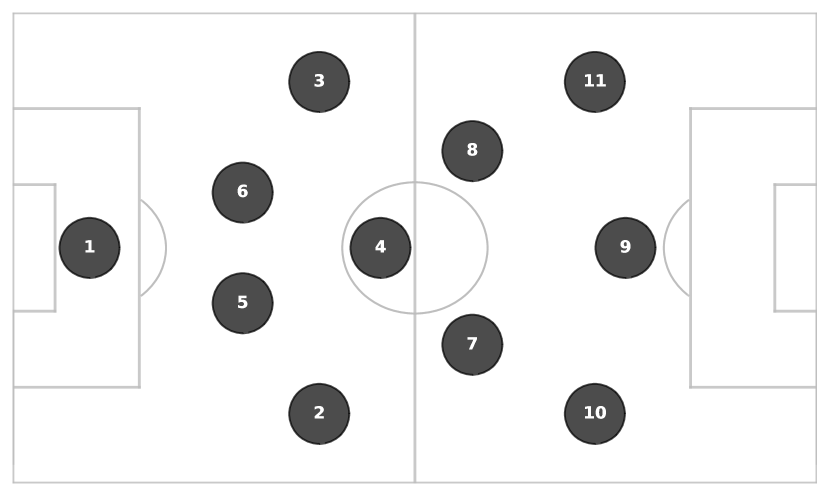
(a) 433 Formation.

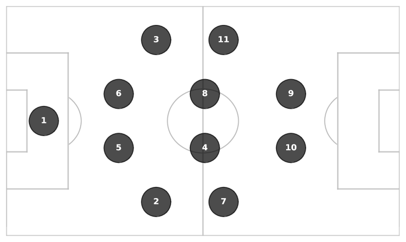
(b) 442 Formation.

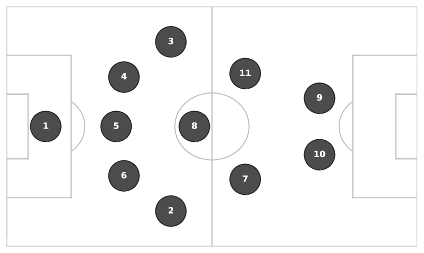
(c) 532 Formation.

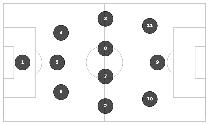
(d) 343 Formation.

Figure 1: The number associated with each position for each group of formations.

3.2 Processing of the data for Hawkes inference

We study our event-based data using Hawkes processes. Doing so, we can gain insights from timestamps of events and information about the spatial coordinates of the ball. For a given team and a list of its games in the same formation cluster, we build a 12-dimensional point process for each game. Each dimension $p\in\{1,\dots,11\}$ records the timestamps of ball touches by the player occupying position $p$, regardless of his identity. The twelfth dimension represents the threat state and is triggered every time there is a ball touch by a player from the considered team in the danger area of the opponent. The danger area is defined as a box around the opposing goal covering 50% of the width of the pitch and 25% of its length, as illustrated in Figure 2. When a player has possession of the ball in this region, the probability of a shot occurring is high, see Singh, (2018) for an estimate of the shot probability at each location on the pitch. Compared to the penalty surface, the danger area is slightly closer to the midfielders and defenders, enabling us to capture more threat events generated by these positions.

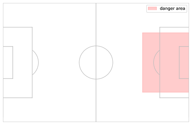
Figure 2: Representation of the danger area.

The following rules are applied when constructing the process:

1. Every time a player in the considered team touches the ball, there is a jump in the dimension $p\in\{1,\dots,11\}$ associated with his position.

2. Every time a player in the considered team touches the ball inside the opposing threat area, there is a jump in the twelfth dimension at the corresponding timestamp. In this case, no jump is recorded in the component associated with the player.

3. Once a threat state is triggered, no jumps or time are recorded until the ball exits the danger area. We resume counting the jumps when the ball is outside the danger area by at least two meters.

4. When the ball is lost (when there is an event where the opposing team has the ball), the time and events are not recorded until the ball is won again. Upon regaining possession, we resume recording the events in our point process by adding a random duration, with an average of twelve seconds, generated from the sum of two exponential distributions of parameter six.

5. We exclude crossing events coming from a free kick or a corner.

Rule 3 is considered to avoid consecutive threat states. We are not interested in the auto-exciting property of the threat events. Therefore, we stop recording once a threat state is achieved and only resume when the team is outside the opposing surface by at least two meters. In Rule 4, we want to avoid having large durations where no event occurs. This is the case every time the considered team loses the ball to the opposition. Thus, the possession times of the opponent are compressed into an average of twelve seconds. The choice of the twelve seconds threshold is based on the average duration between events to which we add another exponential random variable as a penalization for losing the ball. The constructed point process considers possession stretches of the team to be uninterrupted. Rule 5 is implemented because the crossing events are highly correlated with threat events. In particular, the designated set piece taker of each team is naturally responsible for more threats. Therefore, we choose to discard these events to remove bias from our measure of danger creation and ensure fair player comparisons.

Given a collection of games of a team, the point processes built from each game are assembled into one process. An example of the resulting point process is shown in Figure 3. We use information on the timestamps and spatial coordinates on the field to define the threat state. The aim is to extract the causal relationship between player touches. We are interested in identifying the positions where a ball touch is directly correlated to a future jump in the twelfth dimension, which represents a threat. We also want to measure the indirect contribution of a player to the generation of threat through his interaction with other players.

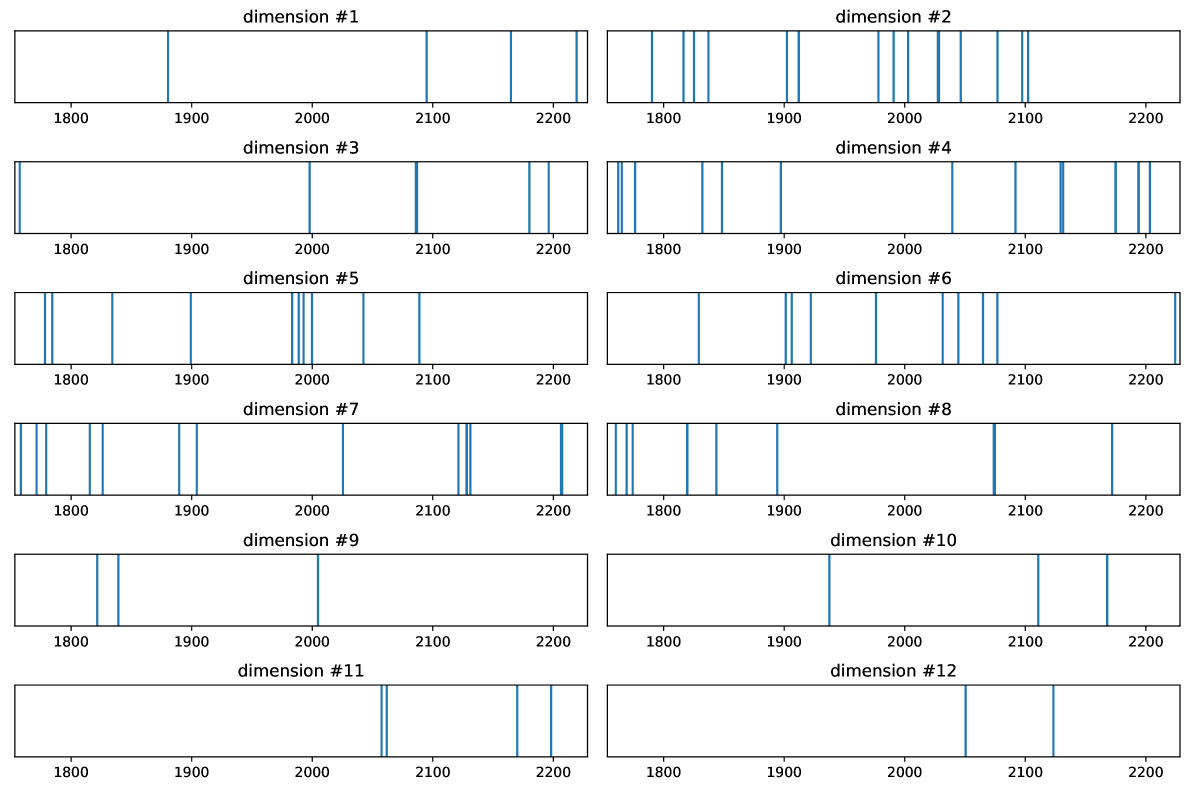
Figure 3: Example of constructed point process.

Remark 3.1.

In the following, we aim at evaluating a player’s performance when he plays in a specific position. To achieve this, we only consider sequences of games where the player in question is playing in that position. We record ball touches in the other positions regardless of the identity of the player occupying them. In Section 5 and Appendix A where we analyze the interactions between the starting eleven players in given teams, we only record sequences of games where the same eleven players play in their respective positions. The way we deal with substitutions is detailed for each case in Sections 5 and 6.

Remark 3.2 (A different twelfth dimension).

In this work, we have incorporated a twelfth dimension that tracks the instances of entering the opposing danger area. This is done because we want to identify the players who are responsible for creating the threat events. Our approach can be extended for various analyses by selecting an alternative twelfth state. For example, we can choose to record the timestamps of ball losses in the twelfth dimension instead of threats. This would enable us to identify the players who are most accountable for losing possession and measure the correlation between their touches and subsequent turnovers.

3.3 Generation of Threat (GoT) indices

The immigration-birth representation of Hawkes processes explained in Section 2 allows us to establish connections between the events in a football match. Essentially, each ball touch or threat event can be seen as an individual in a population, that generates first-generation children of various types - ball touches from other players and threat situations. These offspring, in turn, generate additional ball touches or threat events etc. When we say that an event generates a ball touch or a dangerous situation, we mean that it is responsible for its occurrence. This is a subtle definition because being responsible for an action does not necessarily mean providing the pass that leads to it. In some instances, the second-to-last pass is the most crucial step in creating the dangerous situation. There may even be several events between the generating ball touch and the dangerous action. Our approach eliminates these "noisy" in-between events and associates events through parent-child connections. Hawkes processes impute the responsibility of generating a threat to the most likely parent event, even if it occurred prior to other ball touches. In particular, they allow us to quantify the average number of dangerous actions that can be attributed to a given player.

Using this population representation, we define the following GoT indices to assess the ability of a player to generate threat when he plays in a given position. The first two indices evaluate the impact of one touch of the player whereas the latter two measure the impact of the player’s touches over 90 minutes.

Direct GoT per touch (GoT^d):

A ball touch from the player in position $p$ generates first-generation children of type threat. We refer to these instances as the direct threat events generated by the player touch. We define GoT^d as the average number of these threat events that occur because of one touch from player $p$. This metric describes the intrinsic ability of the player to create dangerous situations. It can be calculated through the estimated branching matrix:

$$\textup{GoT}^{d}(p)=K_{12,p}.$$

Indirect GoT per touch (GoTⁱ):

A ball touch from a given player can be directly responsible for a threat event, but can also generate other ball touches that then generate danger. To quantify the total impact of a single player touch on the danger creation process, we use Proposition 2.1 and consider the matrix

$$M=K(I-K)^{-1}.$$

The coefficient $M_{12,p}$ represents the expected number of threat events where the ball touch from the player $p$ originates the chain of events leading to it. This includes the threat directly generated but also the one resulting from a sequence of other player touches. The difference with the GoT^d index is that we credit the player touch for being at the root of the generation process and not for the crucial creative step.

$$\textup{GoT}^{i}(p)=M_{12,p}.$$

Direct GoT per 90 minutes (GoT${}^{d}_{90}$):

We may want to account for the involvement in the game of a given player by normalizing GoT^d by his expected number of touches. We define the direct GoT per 90 minutes as the expected number of dangerous actions over 90 minutes for which we credit the player:

$$\textup{GoT}_{90}^{d}=\mathbf{E}\left(N_{p}(T)\right)\times\textup{GoT}^{d}(p),$$

where $T=90\textup{ minutes}$. The expected number of touches vector can be approximated thanks to the law of large numbers:

$$\mathbf{E}\left(N(T)\right)\approx(I-K)^{-1}\mu T.$$

Indirect GoT per 90 minutes (GoT${}^{i}_{90}$):

This index measures the expected number of threats over 90 minutes where a given player is involved in the building circuit. We define the indirect GoT per 90 minutes as the average number of threat events subtracted by the average number of threat events if the considered player is removed from the pitch. The GoT${}^{i}_{90}$ index is therefore calculated as follows:

$$\textup{GoT}_{90}^{i}=\mathbf{E}\left(N_{12}(T,K,\mu)-N_{12}(T,K^{(-p)},\mu^{(-p)})\right),$$

where $K^{(-p)}$ is defined as the matrix K where the $p^{th}$ row and $p^{th}$ column are set to zero. Likewise, $\mu^{(-p)}$ is defined as the vector $\mu$ where the $p^{th}$ coordinate is set to 0. The expected number of threats can be approximated using the branching matrix and the baseline intensity $\mu$:

$$\mathbf{E}\left(N_{12}(T,K,\mu)\right)\approx\left((I-K)^{-1}\mu T\right)_{12}.$$

Remark 3.3.

Calculating the GoT${}^{i}_{90}$ by multiplying the GoTⁱ index by the average number of ball touches of the player would overestimate the player’s involvement in danger creation. In fact, we would count multiple times the circuits leading to threat where the player touches the ball more than once.

Additionally, a ball touch from a player can also be responsible for generating ball touches from other players or himself. In this case as well, this is not necessarily achieved through a direct pass. Hawkes processes allow us to estimate the expected number of these generated ball touches. Similar to the GoT^d index definition, the branching coefficient $K_{p_{1},p_{2}}$ indicates the expected number of touches of player $p_{1}$ that happen because a given ball touch from player $p_{2}$ occurred before. The graphical representation of these interaction indices through a graph helps us gain a better understanding of the danger creation process. In particular, it allows us to identify the patterns of play that end in a threat.

4 Maximum Likelihood estimation

4.1 Likelihood of Hawkes process

This section describes briefly parameters estimation for multivariate Hawkes processes, see Ogata et al., (1978); Bonnet et al., 2022b . Consider a $d$-dimensional point process $(N(t))$ on $[0,T]$ with intensity of the form

$$\lambda_{i}(t,\theta^{*})=\mu_{i}^{*}+\sum_{j=1}^{d}\sum_{t_{k}^{(j)}<t}\alpha_{i,j}^{*}\exp\left(-\beta_{i,j}^{*}(t-t_{k}^{(j)})\right),$$

where $\theta^{*}=(\mu^{*},\alpha^{*},\beta^{*})$ are some unknown parameters. Given fixed parameters $\theta=(\mu,\alpha,\beta)$ and a realization of the Hawkes process, the log-likelihood is calculated as follows:

$$\ell(\theta)=\sum_{i=1}^{d}\left(-\int_{0}^{T}\lambda_{i}(s,\theta)ds+\sum_{t_{k}^{(j)}<T}\log\left(\lambda_{i}(t_{k}^{(i)},\theta)\right)\right).$$ (1)

The maximum likelihood estimator is the parameter that maximizes the above function. It can be observed from Equation (1) that the likelihood can be separated into $d$ distinct subfunctions, each dependent on the parameters $\mu_{i}$ and $(\alpha_{i,j},\beta_{i,j})_{j=1,\dots,d}$ for $i$ in $\{1,\dots,d\}$. As a result, the optimization can be performed separately $d$ different times to estimate each subset of parameters. It is shown in Ogata et al., (1978) that this estimator is consistent. Additionally, the log-likelihood can be simplified in the case of exponential kernels and computed in time complexity of $\mathcal{O}\left(d^{2}N(T)\right)$, see Ogata, (1981). For example, for $d=1$ and $T=t_{n}$, the likelihood is given by :

$$\ell(\theta)=\sum\limits_{i=1}^{n}\log\left(\mu+\alpha R(i)\right)-\mu t_{n}+\frac{\alpha}{\beta}\sum_{i=1}^{n}\left(e^{-\beta(t_{n}-t_{i})}-1\right),$$

where $R(i)=\sum\limits_{j=1}^{i-1}e^{-\beta(t_{i}-t_{j})}$ can be computed recursively for i in $\{2,\dots,n\}$ :

$$R(i)=e^{-\beta(t_{i}-t_{i-1})}\left(1+R(i-1)\right).$$

Remark 4.1.

The likelihood function is not concave with respect to $(\beta_{k,l})_{k,l=1,\dots,d}$ in the exponential case. This means that convergence to the global maximum is not guaranteed, especially in large dimensions. Fixing $\beta_{k,l}=\beta_{k}$ for all $l=1,\dots,d$ as proposed by Bonnet et al., 2022b produces very good results for $d=12$. In this case, each of the objective functions is not concave in only one parameter instead of $d$.

Remark 4.2.

In the context of football, the effect of a ball touch on the intensity of the process should last no longer than a few seconds. When $n$ realizations of football matches are concatenated and treated as one long game, the likelihood function should not be altered by much. In fact, the rapid decay of the exponential kernel compared to the duration of games makes the induced error negligible.

4.2 Simulation study

The goal of this section is to evaluate the maximum likelihood estimation using a simulated dataset that reproduces similar dynamics as those in a football game. We want to determine the amount of data required for an accurate estimation of the branching matrix. We also want to assess the model’s ability to detect a null kernel between two dimensions. A null kernel $\phi_{i,j}$ means a jump in dimension $j$ has no exciting effect on dimension $i$. In the context of football, it is particularly informative to detect such an absence of connection between players.

We perform simulations over different horizons. The parameters are sampled as follows:

• $\mu$ is chosen from a uniform random variable over $[0.006,0.01]$.

• $\beta$ is chosen to be constant for all $i,j$ in $\{1,\dots,12\}$ sampled from a uniform random variable over $[0.5,1]$ .

• The $\alpha_{i,j}$ are chosen independently from a geometric distribution of parameter $p=0.4$ scaled by $40$ for all $i,j$ so that $40\%$ of the values are equal to $0$.

Horizon (minutes)	False positive	Error on false negative	Relative error
300	1.1%	0.0054	25.7%
600	0.0%	0.0045	19.3%
1200	0.0%	0.0030	12.4%
2400	0.0%	0.0020	11.4%

Table 1: Accuracy results of the maximum likelihood estimation of Hawkes parameters on the simulated dataset.

Then we fit a 12-dimensional Hawkes process to this data using the algorithm from Bonnet et al., 2022b . We analyze the resulting accuracy as a function of the simulation horizon. Table 1 presents the results through three different metrics:

• False positive: Percentage of branching matrix coefficients $\hat{\alpha}_{i,j}$ wrongly estimated as null when $\alpha_{i,j}>0$. Our estimation correctly detects existing links even for small horizons.

• Error on false negative: Our estimation detects accurately 60% of null links $\alpha_{i,j}=0$. The estimation on the remaining 40% is generally very low as can be seen in Table 1.

• Relative error: The weighted mean absolute percentage error when $\alpha_{i,j}>0$. This metric is defined as the mean absolute error divided by the average value of $\alpha_{i,j}$:

  $$\textup{wMAPE}=\frac{\sum\limits_{i,j}\left|\hat{\alpha}_{i,j}-\alpha_{i,j}\right|\mathbb{1}_{\alpha_{i,j}>0}}{\sum\limits_{i,j}\alpha_{i,j}\mathbb{1}_{\alpha_{i,j}>0}}.$$

The maximum likelihood estimate is good enough for our purposes given the high dimensionality. Figure 4 shows the estimated branching matrix from a simulation of horizon 600 minutes. We observe that the estimated branching matrix appears to correctly approximate the true branching matrix in Figure 5.

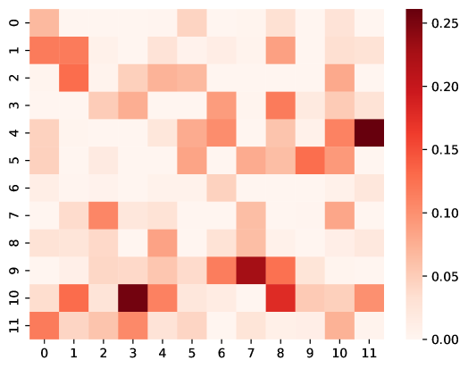
Figure 4: Estimated branching matrix.

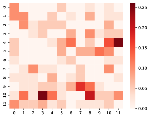
Figure 5: True branching matrix.

Remark 4.3 (Confidence intervals).

Given regularity assumptions on the kernel of the Hawkes process, we can retrieve the rate of convergence of the maximum likelihood estimator and build asymptotic confidence intervals. We do not include confidence interval values here to ease reading but our choice of minimal number of games is dictated by them and the analysis in this section.

5 Analysis of Chelsea FC in the 2016-2017 season

As a first example, we perform our analysis on a selection of Chelsea FC matches from the 2016-2017 season. The team had a stable formation and a constant starting eleven over thirteen games in the Premier League. This is quite convenient because we retrieve a large amount of data where each position $p$ in $\{1,\dots,11\}$ is associated with one player. Similar analysis for Stade Rennais in the 2021-2022 season is provided in Appendix A.

5.1 Selected games

In Table 2, we give the list of selected games for Chelsea FC. In each of these games, the flat 343 formation is used for at least sixty minutes and the starting eleven remains the same:

• Thibaut Courtois.

• Gary Cahill - David Luiz - Cesar Azpilicueta.

• Marcos Alonso - Nemanja Matic - N’Golo Kante - Victor Moses.

• Eden Hazard - Diego Costa - Pedro Rodriguez.

Therefore, we use the data before the first substitution from Chelsea FC in each game to build the counting process.

Date	Opponent	Home or Away	Competition
Oct 15, 2016	Leicester City	Home	English Premier League
Oct 23, 2016	Manchester United	Home	English Premier League
Oct 30, 2016	Southampton	Away	English Premier League
Nov 5, 2016	Everton	Home	English Premier League
Nov 20, 2016	Middlesbrough	Away	English Premier League
Nov 26, 2016	Tottenham Hotspur	Home	English Premier League
Dec 11, 2016	West Bromwich Albion	Home	English Premier League
Jan 4, 2017	Tottenham Hotspur	Away	English Premier League
Jan 22, 2017	Hull City	Home	English Premier League
Feb 4, 2017	Arsenal	Home	English Premier League
Feb 12, 2017	Burnley	Away	English Premier League
Apr 8, 2017	Bournemouth	Away	English Premier League
Apr 30, 2017	Everton	Away	English Premier League

Table 2: List of selected games with the same starting eleven for Chelsea FC.

5.2 Results and discussion

In Table 3, we display the different GoT indices for the Chelsea players. Figure 6 graphically represents the direct interactions between players as well as their GoTⁱ indices and Figure 7 shows the estimated branching matrix. We can identify two buildup schemes along the wings with two triangles: Cahill-Alonso-Matic and Kante-Azpilicueta-Moses. The main channel of communication between both sides is based on the Matic-Kante link.

Below is a list of observations on players:

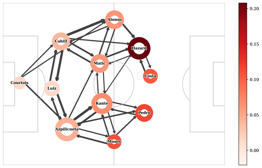
Figure 6: Graph summarizing the interactions between Chelsea players. The width of an arrow from player $p_{1}$ to player $p_{2}$ is proportional to the expected number of touches of player $p_{2}$ generated by one touch from player $p_{1}$. The size of the circle of player $p$ is proportional to the sum of the arrow sizes received, indicating the involvement of the player in the considered games. The color of the circle represents the GoTⁱ index for each player.

Player name	GoTd	GoTi	GoT${}^{d}_{90}$	GoT${}^{i}_{90}$
Eden Hazard	0.16	0.21	14.2	15.0
Victor Moses	0.07	0.11	5.7	7.5
Pedro Rodriguez	0.08	0.12	5.5	6.7
N’Golo Kante	0.02	0.07	2.7	6.2
Nemanja Matic	0.01	0.06	1.5	5.2
Marcos Alonso	0.02	0.06	1.9	5.1
Diego Costa	0.07	0.10	3.6	4.8
Cesar Azpilicueta	0.00	0.04	0.0	4.1
Gary Cahill	0.00	0.04	0.0	3.0
David Luiz	0.00	0.01	0.0	1.0
Thibaut Courtois	0.00	0.01	0.0	0.6

Table 3: Generated threat metrics for the players of Chelsea FC. The table is sorted by GoT${}^{i}_{90}$.

Eden Hazard:

Unsurprisingly, the offensive player, ranked second in the PFA Players’ Player of the Year 2017 award, leads all GoT metrics. In particular, there is no significant difference between his GoT${}^{d}_{90}$ and GoT${}^{i}_{90}$ indices, indicating that his primary way of creating danger is through direct threat. Hazard was well known for his aggressive and direct play as well as for his dribbling.

N’Golo Kante:

Ranking fourth in GoT${}^{i}_{90}$ is evidence to Kante’s important role in Chelsea’s success in the 2016-2017 season. The winner of the PFA Players’ Player of the Year 2017 award is definitely not limited to defense as the numbers show that he is largely involved in danger creation. This is explained by the fact that Kante is a box to box midfielder and that he is at the center of multiple circuits that end in a threat:

• Kante $\rightarrow$ Pedro $\rightarrow$ Threat.

• Kante $\rightarrow$ Moses $\rightarrow$ Pedro $\rightarrow$ Threat.

• Kante $\rightarrow$ Matic $\rightarrow$ Hazard $\rightarrow$ Threat.

David Luiz:

The contribution of the central defender David Luiz in the generation of threat is minimal. This is not surprising as the flat 3-4-3 system relies heavily on the wings. David Luiz naturally passes the ball to either Gary Cahill or Azpilicueta in the build-up to spread the play.

Diego Costa:

Costa generates a small number of threats despite being a striker. This is expected as he is responsible for transforming the goalscoring chances rather than being at the origin of the danger. Moreover, his GoT${}^{i}_{90}$ statistic is particularly low since he has a low number of touches per time unit and many of his touches in the danger zone are not recorded in the constructed counting process.

We can clearly see that considering indirect contribution to threat generation is important for defenders and midfielders. These positions are generally at the base of the danger creation process. They have small GoT^d indices. However, indirect generated threat combined with the consideration of the number of touches allows us to effectively compare players playing in deeper positions.

From the graphical representation in Figure 6, we can identify some patterns that lead to a dangerous situation. When facing a team like Chelsea in the 2016-2017 season, some strategies can be derived from this analysis:

• As illustrated in Figure 6, the right side of Chelsea combines a lot for threat generation and should be disrupted at the root. Azpilicueta should be stopped from feeding the ball to the midfielders or directly to Pedro.

• The left side relies much more on the direct offensive output of Eden Hazard. In fact, all of Gary Cahill, Matic and Marcos Alonso mostly aim at delivering the ball to the left winger. To neutralize the threat of the left side, it is essential to prevent the ball from reaching Hazard. This can be achieved by marking him closely or by constantly closing the passing lanes to him.

• Goalkeeper Courtois is successful in targetting Marcos Alonso directly. This passing pattern should be considered when pressing Chelsea.

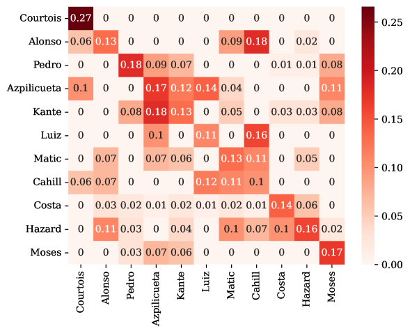
Figure 7: Estimated branching matrix for Chelsea FC.

6 Ligue 1 2021-22 season analysis

In this section, we provide a ranking of players and teams from Ligue 1 in the 2021-2022 season based on their generation of threat. To maintain homogeneity, we only consider for each team the games where they use their main formation cluster, see Table 12 in Appendix B for the list of formation clusters of each team.

6.1 Generated threat to rank players in a position

Each position on the pitch imposes a different role on the player who occupies it. In particular, we cannot expect the same player to produce the same GoT metrics at two different positions. Therefore, we choose to evaluate players when they play in a particular position. This approach will also allow us to determine the optimal position for a player to maximize a GoT metric of interest. Additionally, we apply a filter to consider only players who play at least 600 minutes at a given position, with playing time calculated based on games in which the player features for at least 45 minutes.

Given a player and a position, we record the games in which the player occupies the position. The remaining positions may feature different players at each game. Whenever a player from his team is substituted, we do not consider the rest of the game in the construction of the counting process. We fit a Hawkes process and assign to the player the generated threat indices of his position. Tables 4 and 5 present the top twenty players in Ligue 1 in terms of GoT^d and GoT${}^{i}_{90}$, respectively (see Tables 10 and 11 in Appendix B for the Top 100). We display these two indices because they quantify the two extremes of the danger generation process. GoT^d isolates the direct impact of players while GoT${}^{i}_{90}$ measures their participation in the chain of events leading to threats.

In reference to the results in Section 4.2, one should keep in mind that the fewer minutes a player plays in a position, the less accurate the estimate of his generated threat is. Moreover, our estimation relies on selected games only. When a player has a limited number of minutes in a position, a good GoT metric should be interpreted as a measure of performance across the considered games only. For example, Moses Simon ranking third in GoT^d should not be surprising as he provided seven assists in the 1200 minutes but only gave one more assist in the remaining games when the team plays in a different formation or when he plays in a different position.

Below are some observations based on the results:

Rank	Name	Position	Team	Minutes	GoTd
1	Lionel Messi	10	Paris Saint-Germain	630	0.130
2	Ángel Di María	10	Paris Saint-Germain	1171	0.128
3	Moses Simon	11	Nantes	1222	0.120
4	Kylian Mbappé	9	Paris Saint-Germain	1338	0.110
5	Lionel Messi	9	Paris Saint-Germain	675	0.109
6	Martin Terrier	11	Rennes	1386	0.108
7	Kylian Mbappé	11	Paris Saint-Germain	1066	0.107
8	Romain Faivre	7	Brest	630	0.106
8	Houssem Aouar	7	Lyon	810	0.106
10	Sofiane Boufal	9	Angers	771	0.100
11	Jonathan Ikoné	7	Lille	767	0.096
12	Wissam Ben Yedder	9	Monaco	1625	0.094
13	Franck Honorat	11	Brest	838	0.093
13	Karl Toko-Ekambi	11	Lyon	1855	0.093
15	Benjamin Bourigeaud	10	Rennes	1719	0.092
16	Sofiane Boufal	11	Angers	665	0.091
17	Justin Kluivert	11	Nice	1207	0.090
19	Dimitri Payet	9	Marseille	617	0.088
19	Kevin Gameiro	10	Strasbourg	673	0.088
19	Neymar	11	Paris Saint-Germain	1258	0.088

Table 4: Ranking of Ligue 1 players in terms of GoT^d.

GoT^d vs GoT${}^{i}_{90}$:

GoT^d captures the intrinsic ability of a player to advance the ball to the opponent’s danger area while GoT${}^{i}_{90}$ incorporates possible combinations with teammates. Therefore, the style of play and the ability of teammates can have an impact on the value of GoT${}^{i}_{90}$. These two indices describe different ways to contribute to threat generation and allow us to select different profiles of players. For example, the Paris Saint-Germain midfielder Verratti produces high values of GoT${}^{i}_{90}$ while Moses Simon from FC Nantes features in the top positions in terms of GoT^d.

Jason Berthomier as a surprising pick:

In his only season in Ligue 1, Jason Berthomier delivered excellent values of GoT${}^{i}_{90}$. The Clermont Foot midfielder ranks 43^rd in terms of GoT^d and climbs up to the tenth position in the GoT${}^{i}_{90}$ ranking. This proves that he is consistently involved in the generation of dangerous situations for his team and is successful in feeding the forward players.

Téji Savanier excels in midfield:

Téji Savanier stands out as an interior midfielder in the 433 formation of Montpellier. With eight goals and seven assists, it is no surprise that he is central to the process of threat generation of his team. He ranks eighth in GoT${}^{i}_{90}$ and outperforms many offensive players in the league. This confirms the quality of Téji Savanier and his good performance during the 2021-2022 season.

A defender in the Top 20:

Frederic Guilbert of Strasbourg is a defender who excels at creating threats, ranking 18^th in GoT${}^{i}_{90}$. In fact, his team deploys a 532 formation that provides enough cover for the fullbacks to play offensively. The same holds for Jonathan Clauss who acts almost as a right midfielder in the Lens formation and ranks 33^rd in GoT${}^{i}_{90}$. This is also not surprising as Clauss ranks third in the league in the number of passes that lead to a shot, another proof of his creative play.

A good season from Messi in generated threat:

Despite underperforming in terms of scoring goals, Lionel Messi delivers outstanding values of generated threat both directly given his dribbling and passing quality, and indirectly given his involvement in ball possession. Additionally, we observe that his performance increases slightly when playing in his natural position as a 10 in the 433 formation. The right wing is Messi’s best position as he poses more of a threat cutting inside from the right.

Optimal position for some players:

Romain Faivre stands out in both GoT^d and GoT${}^{i}_{90}$, ranking among the top twenty players. This is in fact expected because, when playing as a right midfielder in the 442 formation of Brest, the player performed well and was involved in six goals in just 660 minutes. Similarly, Houssem Aouar was successful as an interior midfielder in the 433 formation. He scored three and assisted three more in the considered period, earning him a top spot on our list.

A metric that does not value center forwards:

Very few strikers make the Top 20 in the two metrics. This is because the role of some center forwards is to receive the ball in the danger area and not necessarily to be at the origin of the threat. This is even more pronounced when looking at GoT${}^{i}_{90}$. For example, Mbappé, the top scorer in the league, barely makes it to the Top 20. Mbappe is not known for participating in possession and touching the ball a lot but as an aggressive transition player. In contrast, midfielders such as Verratti and Guimarães, that are involved in the build-up of a lot of dangerous situations, feature in the top positions in terms of GoT${}^{i}_{90}$.

Rank	Name	Position	Team	Minutes	GoT${}^{i}_{90}$
1	Lionel Messi	10	Paris Saint-Germain	630	14.911
2	Ángel Di María	10	Paris Saint-Germain	1171	13.218
3	Neymar	11	Paris Saint-Germain	1258	12.724
4	Marco Verratti	4	Paris Saint-Germain	602	12.581
5	Lionel Messi	9	Paris Saint-Germain	675	12.353
6	Romain Faivre	7	Brest	630	10.402
7	Houssem Aouar	7	Lyon	810	10.077
8	Téji Savanier	7	Montpellier	2209	9.608
9	Marco Verratti	8	Paris Saint-Germain	1069	9.446
10	Jason Berthomier	7	Clermont	1244	9.340
11	Benjamin Bourigeaud	10	Rennes	1719	9.211
12	Sofiane Boufal	9	Angers	771	9.100
13	Bruno Guimarães	4	Lyon	900	8.817
14	Dimitri Payet	9	Marseille	617	8.815
15	Moses Simon	11	Nantes	1222	8.790
16	Martin Terrier	11	Rennes	1386	8.639
17	Kylian Mbappé	11	Paris Saint-Germain	1066	8.577
18	Frédéric Guilbert	2	Strasbourg	2428	8.421
19	Ruben Aguilar	2	Monaco	1205	8.019
20	Lovro Majer	7	Rennes	1302	7.927

Table 5: Ranking of Ligue 1 players in terms of GoT${}^{i}_{90}$.

6.2 Ranking the central defenders’ involvement in terms of GoT

To quantify the involvement of central defenders in danger creation, we use the indirect generation of threat per 90 minutes. This is because the direct generation of threat (GoT^d) values are particularly low for defenders and therefore cannot be used to compare players. While GoT${}^{i}_{90}$ is influenced by the quality of the offensive players and team style of play, it also provides valuable information on the role of defenders in the team’s build-up scheme. For instance, a center-back who is technically proficient but avoids taking risks and does not contribute much to ball progression will have a low value of GoT${}^{i}_{90}$. This metric strikes a balance in measuring a player’s intrinsic ability as well as their involvement within the team. Table 6 displays the Top 10 best central defenders with the highest values of GoT${}^{i}_{90}$.

It is no surprise that Marquinhos and Kimpembe take the first two spots, given that they are part of Paris Saint-Germain, the most dominant team in Ligue 1. This is of course due to their technical ability, but there is also a factor due to the high possession values and danger creation ability of their team. The same holds for Nayef Aguerd and Warmed Omari that contribute significantly to ball progression, primarily through accurate long balls. The third-placed is Facundo Medina. The Lens defender is well known for his range of passing and for his ability to switch play from one side to the other. In particular, he ranks tenth in the league in terms of accurate passes per 90 minutes. William Saliba naturally completes the Top 5. The Marseille player excels with the ball at his feet and ranks third in accurate passing in Ligue 1. The player has now moved to Arsenal, a team that likes to play from the back, and continues to deliver in that aspect of the game.

Rank	Name	Position	Team	Minutes	GoT${}^{i}_{90}$
1	Marquinhos	5	Paris Saint-Germain	2340	5.625
2	Presnel Kimpembe	6	Paris Saint-Germain	1840	5.230
3	Facundo Medina	4	Lens	1329	4.953
4	Nayef Aguerd	6	Rennes	1698	4.908
5	William Saliba	5	Marseille	1800	4.652
6	Jason Denayer	6	Lyon	630	4.591
7	Jonathan Gradit	6	Lens	1710	4.535
8	Warmed Omari	5	Rennes	1710	4.407
9	Damien Da Silva	5	Lyon	612	4.182
10	Dante	6	Nice	2880	3.707
11	Duje Caleta-Car	6	Marseille	1397	3.462
12	Lucas Perrin	6	Strasbourg	2329	3.185
13	Kevin Danso	5	Lens	1620	3.105
14	Benoît Badiashile	6	Monaco	975	3.075
15	Castello Lukeba	6	Lyon	1375	3.074
16	Mamadou Sakho	6	Montpellier	1962	2.998
17	Florent Ogier	6	Clermont	2329	2.949
18	Guillermo Maripán	6	Monaco	810	2.916
19	Guillermo Maripán	5	Monaco	605	2.915
20	Jean-Clair Todibo	5	Nice	3123	2.864

Table 6: Ranking of Ligue 1 central defenders in terms of GoT${}^{i}_{90}$.

6.3 GoT^d to rank teams

To verify the consistency of our metrics, we rank Ligue 1 teams based on their aggregate values of GoT^d. This metric can be considered as an indicator of squad quality. For each club, we fit a 12-dimensional Hawkes process to all matches in which they use their primary formation cluster, regardless of the players occupying each position. We then sum the estimated direct threat per touch GoT^d for all the positions.

Table 7 shows the resulting Top 10 based on generated threat. Our metric describes an important part of the offensive performance but obviously does not cover all aspects of the game. Nevertheless, it remains a very good measure of the quality of the team. Our ranking shows a significant $62\%$ Kendall correlation with the realized ranking of Ligue 1. This is achieved while only looking at ball touch and threat event timestamps to infer player abilities. Below are some observations from the ranking:

• Rennes climbs to the second position in our ranking. This is because the team was very attack-minded in the 2021-2022 season and managed to score 82 goals, one of the highest totals in Europe. Their expected threat is proof of their offensive output.

• Olympique Lyonnais, ranked eighth in Ligue 1, still had a very prolific season offensively. They have the third-highest total of goals and the second-highest total of expected goals. It is therefore natural they are fourth with respect to our offensive metric.

Team	GoTd	Ligue 1 ranking	Goals scored
Paris Saint-Germain	0.42	1	90
Rennes	0.41	4	82
Monaco	0.41	3	65
Lyon	0.36	8	66
Marseille	0.36	2	63
Lens	0.30	7	62
Nice	0.28	5	52
Strasbourg	0.26	6	60
Lille	0.26	10	48
Reims	0.26	12	43

Table 7: Top 10 Ligue 1 teams with respect to aggregated GoT^d of starting eleven.

7 Conclusion and future work

In order to measure a player’s ability to create threat in football, we develop model-based metrics that rely on Hawkes processes. These processes provide an easy to interpret way to capture causation between event times. Thanks to this modeling, we are able to identify the players whose touches are most consistently correlated with subsequent threats. We derive four different metrics each describing different ways to create danger. On the one hand, the direct generation of threat metrics GoT^d and GoT${}^{d}_{90}$ allow us to isolate the intrinsic ability of players. On the other hand, GoTⁱ and GoT${}^{i}_{90}$ indicate the indirect contribution to the generation of threat through interactions with other positions. Beyond crediting players for danger generation, our approach can also be used to quantify and visualize the synergies between players on the pitch and identify the patterns that lead to dangerous situations.

We demonstrate our methodology can successfully detect and rank the key players in the 2021-2022 Ligue 1 season, who contribute to their team’s offensive output. The results we find are consistent with the observed performances of the retrieved players, but also reveal some surprising choices. Through the example of Chelsea in the 2016-2017 season, we show that our model-based approach can help teams make data-driven decisions about their tactics. By primarily looking at timestamps of ball touches, we gain a deeper understanding of the threat generation process of a team.

Future work will include exploring the application of our model-based metrics for optimal team selection. In fact, if we are capable of inferring the branching matrix parameters linking players from different teams, we can measure the impact of a potential transfer on the danger creation process. In addition, we can use this framework to capture interactions of players with other game states different from threats. In particular, by replacing the threat events with ball losses, we can effectively analyze the defensive aspect of the game and determine players whose touches are most correlated with a turnover.

Acknowledgment:

The authors thank Anna Bonnet for her help with the estimation of Hawkes processes in large dimensions. They are also grateful to Charlotte Dion and Céline Duval. The authors gratefully acknowledge financial support from the chairs “Machine Learning & Systematic Methods in Finance” and “Deep Finance and Statistics”.

Appendix

Appendix A Stade Rennais

In this appendix, we present a detailed analysis of one of the Ligue 1 teams in the 2021-2022 season.

A.1 Selected games

In the same spirit as Section 5, we choose a collection of games where the formation is the same and starting lineup is as stable as possible. Table 8 shows the selected matches for Stade Rennais. The team plays in a 433 formation in all of these games but the starting eleven is not always exactly the same. In fact, some players are sometimes rotated for a game or two, but we assume that the substitute behaves approximately the same as the starting player. Stade Rennais line up as follows in the selected games, where the main player in each position is in bold:

• Gomis/Alemdar

• Traore - Omari/Bade - Aguerd/Bade/Santamaria - Truffert/Meling

• Majer - Santamaria/Martin - Tait

• Bourigeaud - Laborde/Guirassy - Terrier

We construct a 12-dimensional counting process from the selected Stade Rennais games regardless of the players starting. We use the data from each game as long as the eleven players on the pitch correspond to the scheme provided above. We then fit a 12-dimensional Hawkes process and associate the estimated metrics of each position with the main player occupying it.

Date	Opponent	Home or Away	Competition
May 11, 2022	Nantes	Away	French Ligue 1
Apr 2, 2022	Nice	Away	French Ligue 1
May 14, 2022	Marseille	Home	French Ligue 1
Dec 22, 2021	Monaco	Away	French Ligue 1
Mar 20, 2022	Metz	Home	French Ligue 1
Apr 15, 2022	Monaco	Home	French Ligue 1
Apr 30, 2022	St Etienne	Home	French Ligue 1
Apr 24, 2022	Lorient	Home	French Ligue 1
Nov 20, 2021	Montpellier	Home	French Ligue 1
May 21, 2022	Lille	Away	French Ligue 1
Nov 7, 2021	Lyon	Home	French Ligue 1

Table 8: List of selected games for Stade Rennais F.C.

A.2 Results and discussion

In Table 9, we rank the Stade Rennais players with respect to generated threat metrics. Figure 8 graphically represents the direct interactions between them and Figure 9 displays the estimated branching matrix.

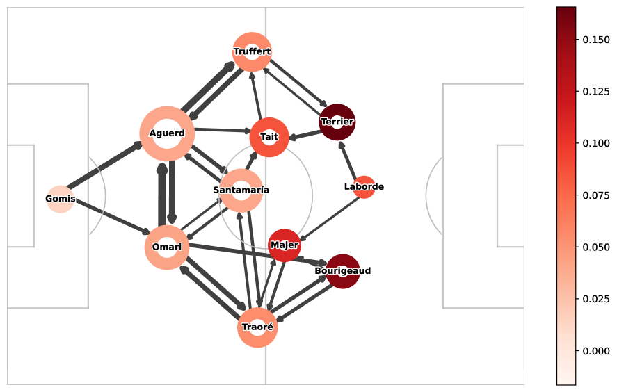
Figure 8: Graph summarizing the interactions between Stade Rennais players. The width of an arrow from player $p_{1}$ to player $p_{2}$ is proportional to the expected number of touches of player $p_{2}$ generated by one touch from player $p_{1}$. The size of the circle of player $p$ is proportional to the sum of the arrow sizes received, indicating the involvement of the player in the considered games. The color of the circle represents the GoTⁱ index for each player.

We can see that the team adopts a 433 shape that progresses mainly through the wings. The danger creation is asymmetric with more combinations occurring on the right side, where Majer is the most creative midfielder. Interestingly, despite being a central midfielder, Flavien Tait delivers a large value of GoT${}^{i}_{90}$, indicating that he is a significant contributor to the team’s offensive efforts. In contrast, although Santamaria has more possession, he has limited involvement in creating threats. This difference in their threat generation can be attributed to their distinct roles on the field. On one hand, Tait is a more box-to-box midfielder who frequently projects forward and has a considerable direct threat metric. On the other hand, Santamaria belongs to a class of defensive midfielders who act as anchor points. They participate in the buildup close to the center backs and have limited interactions with the forward positions.

The main threat sources are Bourigeaud, Majer, and Terrier. These three players are outstanding going forward. Terrier is the leader of the team in goalscoring and ranks third in Ligue 1 but seems to be involved in danger creation as well. Bourigeaud generating the most threat is not surprising since he is the creative force of the team. In fact, he ranks first in the league in terms of key passes with 3.2 per game, and first in accurate crosses with 104 in the season.

As expected, the center backs have zero direct threat contribution. However, in terms of indirect threat per 90 minutes GoT${}^{i}_{90}$, Aguerd and Omari rank fourth and sixth in the team respectively. The pair generates danger through their involvement in team build-up and possession. In particular, Aguerd and Omari are comfortable with the ball at their feet and rank eighth and twentieth in the league, respectively, in the number of passes per game with high success rates.

Player name	GoTd	GoTi	GoT${}^{d}_{90}$	GoT${}^{i}_{90}$
Benjamin Bourigeaud	0.14	0.16	11.8	12.6
Martin Terrier	0.13	0.17	8.6	9.5
Lovro Majer	0.08	0.11	6.9	8.1
Flavien Tait	0.06	0.09	5.5	7.2
Adrien Truffert	0.02	0.06	2.4	5.2
Hamari Traoré	0.01	0.05	1.5	4.6
Nayef Aguerd	0.00	0.04	0.0	4.5
Baptiste Santamaría	0.00	0.05	0.4	4.3
Warmed Omari	0.00	0.04	0.0	4.0
Gaëtan Laborde	0.04	0.08	2.0	3.0
Alfred Gomis	0.00	0.01	0.0	0.7

Table 9: Generated threat metrics for the players of Stade Rennais. The table is sorted by GoT${}^{i}_{90}$.

Finally, we can observe from Figure 8 some remarkable circuits that lead to dangerous situations. These patterns of play should be taken into account by an opposing team when facing Stade Rennais:

• Aguerd $\rightarrow$ Truffert $\rightarrow$ Terrier $\rightarrow$ Threat.

• Terrier $\rightarrow$ Tait $\rightarrow$ Threat. Terrier is highly effective in generating direct threats, but he also frequently combines with Flavien Tait to create danger. Similarly, Bourigeaud often gives the ball to Lovro Majer to generate indirect threat.

• Omari $\rightarrow$ Traoré $\rightarrow$ Bourigeaud $\rightarrow$ Threat.

• Omari $\rightarrow$ Bourigeaud $\rightarrow$ Threat. This is a straightforward pattern from defense to attack that should be controlled. Omari is highly successful in progressing the ball, both through slow build-up play by passing the ball to the right-back Traoré, as well as through fast transitions with direct passes to Bourigeaud.

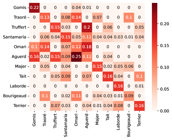
Figure 9: Estimated branching matrix for Stade Rennais.

Appendix B Top 100 ranking of Ligue 1 player in terms of GoT

Rank	Name	Position	Team	Minutes	GoTd
1	Lionel Messi	10	Paris Saint-Germain	630	0.130
2	Ángel Di María	10	Paris Saint-Germain	1171	0.128
3	Moses Simon	11	Nantes	1222	0.120
4	Kylian Mbappé	9	Paris Saint-Germain	1338	0.110
5	Lionel Messi	9	Paris Saint-Germain	675	0.109
6	Martin Terrier	11	Rennes	1386	0.108
7	Kylian Mbappé	11	Paris Saint-Germain	1066	0.107
8	Romain Faivre	7	Brest	630	0.106
8	Houssem Aouar	7	Lyon	810	0.106
10	Sofiane Boufal	9	Angers	771	0.100
11	Jonathan Ikoné	7	Lille	767	0.096
12	Wissam Ben Yedder	9	Monaco	1625	0.094
13	Franck Honorat	11	Brest	838	0.093
13	Karl Toko-Ekambi	11	Lyon	1855	0.093
15	Benjamin Bourigeaud	10	Rennes	1719	0.092
16	Sofiane Boufal	11	Angers	665	0.091
17	Justin Kluivert	11	Nice	1207	0.090
19	Dimitri Payet	9	Marseille	617	0.088
19	Kevin Gameiro	10	Strasbourg	673	0.088
19	Neymar	11	Paris Saint-Germain	1258	0.088
21	Jodel Dossou	10	Clermont	1762	0.086
22	Lucas Da Cunha	10	Clermont	606	0.084
22	Jim Allevinah	11	Clermont	858	0.084
24	Frédéric Guilbert	2	Strasbourg	2428	0.082
25	Armand Laurienté	9	Lorient	842	0.080
26	Ludovic Blas	7	Nantes	810	0.078
27	Gaël Kakuta	9	Lens	976	0.077
28	Arnaud Kalimuendo-Muinga	11	Lens	724	0.075
29	Cengiz Ünder	10	Marseille	1047	0.074
29	Florent Mollet	10	Montpellier	1269	0.074
31	Téji Savanier	7	Montpellier	2209	0.071
32	Ghislain Konan	3	Reims	1007	0.070
33	Lovro Majer	7	Rennes	1302	0.068
34	Kevin Volland	7	Monaco	1131	0.067
34	Jonathan Clauss	2	Lens	1940	0.067
36	Angelo Fulgini	8	Angers	630	0.066
36	Andy Delort	10	Nice	1478	0.066
38	Javairô Dilrosun	9	Bordeaux	675	0.064
39	Vanderson	10	Monaco	619	0.061
40	Lucas Paquetá	7	Lyon	1248	0.060
40	Burak Yilmaz	9	Lille	1900	0.060
43	Jonathan Bamba	11	Lille	1763	0.059
43	Thomas Foket	2	Reims	631	0.059
43	Jason Berthomier	7	Clermont	1244	0.059
45	Amine Gouiri	9	Nice	1749	0.058
46	Gaëtan Laborde	9	Rennes	1305	0.057
47	Ibrahima Sissoko	7	Strasbourg	826	0.055
48	Jonathan David	10	Lille	2072	0.054
49	Dimitri Lienard	3	Strasbourg	1728	0.050
51	Flavien Tait	8	Rennes	1129	0.046

Rank	Name	Position	Team	Minutes	GoTd
51	Florian Sotoca	10	Lens	1119	0.046
51	Jérémy Le Douaron	10	Brest	759	0.046
53	Andy Delort	9	Nice	795	0.045
55	Youcef Atal	2	Nice	1032	0.044
55	Randal Kolo Muani	9	Nantes	876	0.044
55	Stephy Mavididi	11	Montpellier	1585	0.044
55	Aleksandr Golovin	11	Monaco	607	0.044
58	Elbasan Rashani	11	Clermont	1588	0.043
59	Mohamed Bayo	9	Clermont	2331	0.042
60	Abdu Conté	3	Troyes	695	0.041
60	Sanjin Prcic	11	Strasbourg	652	0.041
64	Bruno Guimarães	4	Lyon	900	0.040
64	Anthony Caci	3	Strasbourg	1400	0.040
64	Kevin Gameiro	9	Strasbourg	1458	0.040
64	Hicham Boudaoui	7	Nice	1304	0.040
64	Gerson	8	Marseille	704	0.040
67	Sofiane Diop	11	Monaco	631	0.039
68	Igor Silva	2	Lorient	1197	0.038
69	Renato Sanches	8	Lille	951	0.037
69	Issa Kaboré	2	Troyes	1679	0.037
71	Mohamed-Ali Cho	10	Angers	807	0.035
71	Angelo Fulgini	9	Angers	751	0.035
74	Akim Zedadka	2	Clermont	3330	0.034
74	Pol Lirola	2	Marseille	863	0.034
74	Adrien Thomasson	7	Strasbourg	1853	0.034
76	Habib Diallo	10	Strasbourg	859	0.033
76	Xavier Chavalerin	11	Troyes	949	0.033
78	Jean-Ricner Bellegarde	11	Strasbourg	1454	0.032
78	Maxence Caqueret	8	Lyon	1389	0.032
80	Vital N’Simba	3	Clermont	2731	0.031
80	Ruben Aguilar	2	Monaco	1205	0.031
83	Seko Fofana	8	Lens	1861	0.030
83	Ismail Jakobs	3	Monaco	650	0.030
83	Terem Moffi	10	Lorient	911	0.030
87	Valère Germain	9	Montpellier	1083	0.029
87	Stéphane Bahoken	10	Angers	657	0.029
87	Youssouf Fofana	8	Monaco	1116	0.029
87	Mattéo Guendouzi	7	Marseille	1350	0.029
87	Ludovic Ajorque	10	Strasbourg	1334	0.029
90	Ludovic Ajorque	9	Strasbourg	1243	0.028
90	Marco Verratti	4	Paris Saint-Germain	602	0.028
93	Baptiste Santamaría	8	Rennes	675	0.027
93	Vincent Le Goff	3	Lorient	1440	0.027
93	Ricardo Mangas	3	Bordeaux	613	0.027
96	Caio Henrique	3	Monaco	1454	0.026
96	Mihailo Ristic	3	Montpellier	1150	0.026
96	Junior Sambia	2	Montpellier	732	0.026
98	Souleyman Doumbia	3	Angers	1797	0.025
98	Przemyslaw Frankowski	3	Lens	1191	0.025
100	Florian Tardieu	8	Troyes	1530	0.024

Table 10: Ranking of Ligue 1 players in terms of GoT^d.

Rank	Name	Position	Team	Minutes	GoT${}^{i}_{90}$
1	Lionel Messi	10	Paris Saint-Germain	630	14.911
2	Ángel Di María	10	Paris Saint-Germain	1171	13.218
3	Neymar	11	Paris Saint-Germain	1258	12.724
4	Marco Verratti	4	Paris Saint-Germain	602	12.581
5	Lionel Messi	9	Paris Saint-Germain	675	12.353
6	Romain Faivre	7	Brest	630	10.402
7	Houssem Aouar	7	Lyon	810	10.077
8	Téji Savanier	7	Montpellier	2209	9.608
9	Marco Verratti	8	Paris Saint-Germain	1069	9.446
10	Jason Berthomier	7	Clermont	1244	9.340
11	Benjamin Bourigeaud	10	Rennes	1719	9.211
12	Sofiane Boufal	9	Angers	771	9.100
13	Bruno Guimarães	4	Lyon	900	8.817
14	Dimitri Payet	9	Marseille	617	8.815
15	Moses Simon	11	Nantes	1222	8.790
16	Martin Terrier	11	Rennes	1386	8.639
17	Kylian Mbappé	11	Paris Saint-Germain	1066	8.577
18	Frédéric Guilbert	2	Strasbourg	2428	8.421
19	Ruben Aguilar	2	Monaco	1205	8.019
20	Lovro Majer	7	Rennes	1302	7.927
21	Lucas Da Cunha	10	Clermont	606	7.882
22	Kylian Mbappé	9	Paris Saint-Germain	1338	7.733
23	Ghislain Konan	3	Reims	1007	7.721
24	Sanjin Prcic	11	Strasbourg	652	7.624
25	Sofiane Boufal	11	Angers	665	7.547
26	Lucas Paquetá	7	Lyon	1248	7.450
27	Karl Toko-Ekambi	11	Lyon	1855	7.365
28	Jonathan Ikoné	7	Lille	767	7.285
29	Franck Honorat	11	Brest	838	7.207
30	Achraf Hakimi	2	Paris Saint-Germain	1781	7.125
31	Idrissa Gueye	8	Paris Saint-Germain	662	7.090
32	Dimitri Lienard	3	Strasbourg	1728	7.050
33	Gerson	8	Marseille	704	7.016
34	Vanderson	10	Monaco	619	6.939
35	Ibrahima Sissoko	7	Strasbourg	826	6.892
36	Ludovic Blas	7	Nantes	810	6.816
37	Gaël Kakuta	9	Lens	976	6.802
38	Jonathan Clauss	2	Lens	1940	6.757
39	Justin Kluivert	11	Nice	1207	6.700
40	Flavien Tait	8	Rennes	1129	6.671
41	Kevin Gameiro	10	Strasbourg	673	6.569
42	Florent Mollet	10	Montpellier	1269	6.465
43	Angelo Fulgini	8	Angers	630	6.459
44	Renato Sanches	8	Lille	951	6.427
45	Henrique	3	Lyon	619	6.385
46	Danilo Pereira	4	Paris Saint-Germain	879	6.346
47	Pol Lirola	2	Marseille	863	6.327
48	Jim Allevinah	11	Clermont	858	6.303
49	Youcef Atal	2	Nice	1032	6.258
50	Maxence Caqueret	8	Lyon	1389	6.229

Rank	Name	Position	Team	Minutes	GoT${}^{i}_{90}$
51	Vital N’Simba	3	Clermont	2731	6.066
52	Anthony Caci	3	Strasbourg	1400	6.023
53	Emerson	3	Lyon	1848	6.019
54	Aleksandr Golovin	11	Monaco	607	5.973
55	Birger Meling	3	Rennes	776	5.936
56	Juan Bernat	3	Paris Saint-Germain	777	5.929
57	Jodel Dossou	10	Clermont	1762	5.864
58	Caio Henrique	3	Monaco	1454	5.855
59	Jonas Martin	4	Rennes	1115	5.810
60	Thomas Foket	2	Reims	631	5.805
61	Jonathan Bamba	11	Lille	1763	5.632
62	Marquinhos	5	Paris Saint-Germain	2340	5.625
63	Florian Sotoca	10	Lens	1119	5.598
64	Jordan Ferri	8	Montpellier	2129	5.516
65	Aurélien Tchouaméni	4	Monaco	1620	5.431
66	Malo Gusto	2	Lyon	1369	5.382
67	Cheick Oumar Doucouré	7	Lens	1350	5.372
68	Armand Laurienté	9	Lorient	842	5.345
69	Akim Zedadka	2	Clermont	3330	5.281
70	Presnel Kimpembe	6	Paris Saint-Germain	1840	5.230
71	Ismail Jakobs	3	Monaco	650	5.199
72	Fábio	3	Nantes	726	5.154
73	Thilo Kehrer	2	Paris Saint-Germain	632	5.144
74	Cengiz Ünder	10	Marseille	1047	5.079
75	Léo Dubois	2	Lyon	1246	5.060
76	Mattéo Guendouzi	7	Marseille	1350	4.995
77	Facundo Medina	4	Lens	1329	4.953
78	Adrien Thomasson	7	Strasbourg	1853	4.921
79	Nayef Aguerd	6	Rennes	1698	4.908
80	Abdu Conté	3	Troyes	695	4.891
81	Javairô Dilrosun	9	Bordeaux	675	4.845
82	Hamari Traoré	2	Rennes	1878	4.836
83	Przemyslaw Frankowski	3	Lens	1191	4.778
84	Wissam Ben Yedder	9	Monaco	1625	4.685
85	Vincent Le Goff	3	Lorient	1440	4.669
86	Valentin Rongier	2	Marseille	899	4.668
87	Angelo Fulgini	9	Angers	751	4.661
88	William Saliba	5	Marseille	1800	4.652
89	Boubacar Kamara	4	Marseille	1497	4.636
90	Nuno Mendes	3	Paris Saint-Germain	1246	4.599
91	Jason Denayer	6	Lyon	630	4.591
92	Baptiste Santamaría	8	Rennes	675	4.536
93	Jonathan Gradit	6	Lens	1710	4.535
94	Youssouf Fofana	8	Monaco	1116	4.517
95	Florian Tardieu	8	Troyes	1530	4.496
96	Jordan Lotomba	2	Nice	1410	4.454
97	Mihailo Ristic	3	Montpellier	1150	4.439
98	Warmed Omari	5	Rennes	1710	4.407
99	Melvin Bard	3	Nice	2470	4.350
100	Seko Fofana	8	Lens	1861	4.345

Table 11: Ranking of Ligue 1 players in terms of GoT${}^{i}_{90}$.

Team	Formation cluster
Angers	3
Bordeaux	3
Brest	2
Clermont	1
Lens	3
Lille	2
Lorient	3
Lyon	1
Marseille	1
Metz	3
Monaco	1
Montpellier	1
Nantes	1
Nice	2
Paris Saint-Germain	1
Reims	3
Rennes	1
St Etienne	4
Strasbourg	3
Troyes	4

Table 12: The main formation clusters for each team in Ligue 1 in the 2021-2022 season.

References

- Adamopoulos, (1976) Adamopoulos, L. (1976). Cluster models for earthquakes: Regional comparisons. Journal of the International Association for Mathematical Geology, 8:463–475.
- (2) Bonnet, A., Dion-Blanc, C., Gindraud, F., and Lemler, S. (2022a). Neuronal network inference and membrane potential model using multivariate Hawkes processes. Journal of Neuroscience Methods, 372:109550.
- (3) Bonnet, A., Herrera, M. M., and Sangnier, M. (2022b). Inference of multivariate exponential Hawkes processes with inhibition and application to neuronal activity. arXiv preprint arXiv:2205.04107.
- Brémaud, (1981) Brémaud, P. (1981). Point processes and queues: martingale dynamics, volume 50. Springer.
- Green, (2012) Green, S. (2012). Assessing the performance of Premier League goalscorers. https://www.statsperform.com/resource/assessing-the-performance-of-premier-league-goalscorers/.
- (6) Hawkes, A. G. (1971a). Point spectra of some mutually exciting point processes. Journal of the Royal Statistical Society: Series B (Methodological), 33(3):438–443.
- (7) Hawkes, A. G. (1971b). Spectra of some self-exciting and mutually exciting point processes. Biometrika, 58(1):83–90.
- Hawkes and Oakes, (1974) Hawkes, A. G. and Oakes, D. (1974). A cluster process representation of a self-exciting process. Journal of Applied Probability, 11(3):493–503.
- Jaisson and Rosenbaum, (2015) Jaisson, T. and Rosenbaum, M. (2015). Limit theorems for nearly unstable Hawkes processes. The Annals of Applied Probability, 25(2).
- Lambert et al., (2018) Lambert, R. C., Tuleau-Malot, C., Bessaih, T., Rivoirard, V., Bouret, Y., Leresche, N., and Reynaud-Bouret, P. (2018). Reconstructing the functional connectivity of multiple spike trains using Hawkes models. Journal of neuroscience methods, 297:9–21.
- Ogata, (1981) Ogata, Y. (1981). On lewis’ simulation method for point processes. IEEE transactions on information theory, 27(1):23–31.
- Ogata, (1988) Ogata, Y. (1988). Statistical models for earthquake occurrences and residual analysis for point processes. Journal of the American Statistical association, 83(401):9–27.
- Ogata et al., (1978) Ogata, Y. et al. (1978). The asymptotic behaviour of maximum likelihood estimators for stationary point processes. Annals of the Institute of Statistical Mathematics, 30(1):243–261.
- Singh, (2018) Singh, K. (2018). Introducing Expected Threat (xT). https://karun.in/blog/expected-threat.html.
- Whitmore, (2021) Whitmore, J. (2021). What Are Expected Assists (xA)? https://theanalyst.com/eu/2021/03/what-are-expected-assists-xa/.