Nonergodic measurements of qubit frequency noise

Abstract

Slow fluctuations of a qubit frequency are one of the major problems faced by quantum computers. To understand their origin it is necessary to go beyond the analysis of their spectra. We show that characteristic features of the fluctuations can be revealed using comparatively short sequences of periodically repeated Ramsey measurements, with the sequence duration smaller than needed for the noise to approach the ergodic limit. The outcomes distribution and its dependence on the sequence duration are sensitive to the nature of noise. The time needed for quantum measurements to display quasi-ergodic behavior can strongly depend on the measurement parameters.

I Introduction

Due to the probabilistic nature of quantum measurements, many currently implemented quantum algorithms rely on repeatedly running a quantum computer. It is important that the qubit parameters remain essentially the same between the runs. This imposes a constraint on comparatively slow fluctuations of the qubit parameters, in particular qubit frequencies, and on developing means of revealing and charactetizing such fluctuations.

Slow qubit frequency fluctuations have been a subject of intense studies [1, 2, 3, 4, 5, 6, 7, 8, 9, 10, 11, 12, 13, 14, 15, 16, 17, 18, 19, 20, 21, 22, 23]. Of primary interest has been their spectrum, although their statistics has also attracted interest [24, 25, 26, 27, 28, 29, 30, 31, 32, 33]. This statistics is important as it may help to reveal the source of the underlying noise. In particular, fluctuations from the coupling to a few TLSs should be non-Gaussian [34, 35, 36, 37, 38, 25, 39, 30, 40]. The fluctuation statistics has been often described in terms of higher-order time correlators or their Fourier transforms, bi-spectra and high-order spectra. Most work thus far has been done on fluctuations induced by noise with the correlation time smaller than the qubit decay time.

Here we show that important information about qubit frequency fluctuations can be extracted from what we call nonergodic measurements. The idea is to perform $M$ successive qubit measurements (for example, Ramsey measurements) over time longer than the qubit decay time but shorter than the noise correlation time. The measurement outcomes are determined by the instantaneous state of the noise source, for example, by the instantaneous TLSs’ states. They vary from one series of $M$ measurements to another. Thus the outcome distribution reflects the distribution of the noise source over its states. It provides information that is washed out in the ensemble averaging inherent to ergodic measurements.

Closely related is the question of how long should a quantum measurement sequence be to reach the ergodic limit in which the noise source explores all its states. Does the measurement duration depend on the type and parameters of the measurement, not only the noise source properties, and if so, on which parameters?

A convenient and frequently used method of performing successive measurements is to repeat them periodically. In this case the duration of data acquisition of $M$ measurements is $\propto M$. For the measurements to be nonergodic it should suffice for this duration to be smaller than the noise correlation time. This imposes a limitation on $M$ from above. The limitation on $M$ from below is imposed by the uncertainty that comes from the quantum nature of the measurements and thus requires statistical averaging over the outcomes.

We consider a periodic sequence of Ramsey measurements sketched in Fig. 1. At the beginning of a measurement the qubit, initially in the ground state $\ket{0}$, is rotated about the $y$-axis of the Bloch sphere by $\pi/2$, which brings it to the state $(\ket{0}+\ket{1})/\sqrt{2}$. After time $t_{R}$ the rotation is repeated and is followed by a projective measurement of finding the qubit in state $\ket{1}$. The qubit is then reset to $\ket{0}$, cf. [41]. In our scheme the measurements are repeated $M\gg 1$ times, with period $t_{\mathrm{cyc}}$.

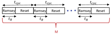
Figure 1: Schematics of $M$ Ramsey measurements. In each measurement the qubit phase is accumulated over time $t_{R}$. The measurements give the probability $p$ to find the qubit in state $\ket{1}$. After a measurement the qubit is reset to state $\ket{0}$. The measurements are repeated with period $t_{\mathrm{cyc}}$.

The outcome of a $k$th Ramsey measurement $x_{k}$ is 0 or 1. The probability $p$ to find $x_{k}=1$ is determined by the qubit phase accumulated over time $t_{R}$. This phase comes from the detuning of the qubit frequency from the frequency of the reference drive and from the noise-induced qubit frequency fluctuations $\delta\omega_{\mathrm{q}}(t)$. The detuning is controllable, and we will use $\phi_{R}$ to indicate the phase that comes from it. The Hamiltonian $H_{\mathrm{fl}}$ that describes frequency fluctuations and the phase $\theta_{k}$ accumulated in the $k$th measurement due to these fluctuations have the form

$$H_{\mathrm{fl}}=-\frac{1}{2}\delta\omega_{\mathrm{q}}(t)\sigma_{z},\qquad\theta_{k}=\int_{kt_{\mathrm{cyc}}}^{kt_{\mathrm{cyc}}+t_{R}}\delta\omega_{\mathrm{q}}(t)dt\ .$$ (1)

Here we have set $\hbar=1$; we associate the Pauli operators $\sigma_{x,y,z}$ with the operators acting on the qubit states. We are interested in slow frequency fluctuations. The correlation time of $\delta\omega_{\mathrm{q}}(t)$ is $\gtrsim t_{\mathrm{cyc}}$ and may significantly exceed the reciprocal qubit decay rate.

In terms of the phases $\theta$ and $\phi_{R}$, the probability to have $x_{k}=1$ is [42]

$$p(\theta)=\frac{1}{2}\left[1+e^{-t_{R}/T_{2}}\cos(\phi_{R}+\theta)\right],$$ (2)

where $T_{2}^{-1}$ is the qubit decoherence rate due to fast processes leading to decay and dephasing. In the absence of qubit frequency noise $\theta=0$ for all $M$ measurements and the distribution of the measurement outcomes is a binomial distribution [43]. Because of the frequency noise, the phase $\theta$ in Eq. (2) becomes random, changing from one measurement to another, and thus the probability $p(\theta)$ also becomes random. Then the outcomes distribution is determined not just by the quantum randomness, but also by the distribution of the values of $\theta$.

The randomness of the phase is captured by the probability $\rho(m|M)$ to have $x_{k}=1$ as a measurement outcome $m$ times in $M$ measurements, $\rho(m|M)=\mathrm{Prob}(\sum_{k=1}^{M}x_{k}=m)$. We consider $\rho(m|M)$ for periodically repeated measurements, see Fig. 1. If the frequency noise has correlation time small compared to the period $t_{\mathrm{cyc}}$, the phases $\theta_{k}$ in successive measurements are uncorrelated. Then $\rho(m|M)$ is still given by a binomial distribution,

$$\rho_{\mathrm{binom}}(m|M)=\binom{M}{m}r_{1}^{m}(1-r_{1})^{M-m},$$ (3)

where $r_{1}\equiv\langle x_{k}\rangle=\langle p(\theta)\rangle_{\theta}$; here $\langle...\rangle_{\theta}$ indicates averaging over realizations of $\theta$. For large $M$ this distribution is close to a Gaussian peak centered at $r_{1}$.

We are interested in the opposite case of slow frequency noise. Here the distribution $\rho(m|M)$ can strongly deviate from the binomial distribution. The deviation becomes pronounced and characteristic of the noise if $Mt_{\mathrm{cyc}}$ is comparable or smaller than the noise correlation time while $M$ is still large.

The effect is particularly clear in the static limit, where the noise does not change over time $Mt_{\mathrm{cyc}}$, i.e., the phase $\theta$ remains constant during $M$ measurements. Even though $\theta$ is constant, its value $\theta=\theta(\ell)$ is random, it varies from one series of $M$ measurements to another; here $\ell$ enumerates the series, and we assume that noise correlations decay between successive series. The probability $P[\theta(\ell)]$ to have a given $\theta(\ell)$ is determined by the noise statistics. The distribution of the outcomes $\rho(m|M)$ is obtained by averaging the results of multiply repeated series of $M$ measurements. Extending the familiar arguments that lead to Eq. (3), we find

$$\rho(m|M)=\binom{M}{m}\sum_{\ell}P[\theta(\ell)]p^{m}[\theta(\ell)]$$

$$\times\{1-p[\theta(\ell)]\}^{M-m}$$ (4)

The distribution (I) directly reflects the distribution of the noise over its states. In particular, if the values of $\theta(\ell)$ are discrete and well-separated (see an example below), $\rho(m|M)$ has a characteristic fine structure with peaks located at $m\approx Mp[\theta(\ell))]$ for $M\gg 1$; the peak heights are determined by $P[\theta(\ell)]$.

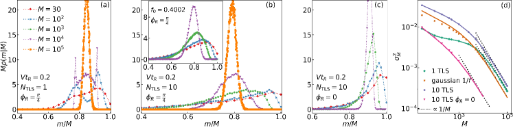
Figure 2: Transition from nonerogidc to ergodic behavior with the increasing number of measurements. Red diamonds, blue crosses, green dots, purple triangles, and orange squares in panels (a)-(c) show $\rho(m|M)$ for $M=30,10^{2},10^{3},10^{4}$ and $10^{5}$, respectively. The parameter of the dispersive qubit-to-TLS coupling is $Vt_{R}=0.2$. The control parameter $\phi_{R}$ is $\pi/4$ in panels (a) and (b). (a) Coupling to a single symmetric TLS with the scaled switching rate $Wt_{R}=1.2\times 10^{-4}$. (b) Coupling to 10 symmetric TLSs with the switching rates $W^{(n)}t_{R}=\exp(-3n/4)$, $n=3,4,\ldots,12$. The inset shows the results for Gaussian $1/f$-type noise described in the text, $f_{0}=\langle\delta\omega_{q}^{2}\rangle t_{R}^{2}$. (c) Coupling to the same 10 TLSs as in panel (b), but for $\phi_{R}=0$. (d) The variance of $\rho(m|M)$ for the data in panels (a)-(c); the solid lines show the theory, Eq. (I), the data points show the results of the simulations. The dashed lines show the ergodic limit.

An important example of slow frequency noise is the noise that results from dispersive coupling to a set of slowly switching TLSs,

$$\delta\omega_{\mathrm{q}}(t)=\sum_{n}V^{(n)}{}\hat{\tau}_{z}^{(n)}.$$ (5)

Here $n=1,...,N_{\mathrm{TLS}}$ enumerates the TLSs, $\hat{\tau}_{z}^{(n)}$ is the Pauli operator of the $n$th TLS, and $V^{(n)}{}$ is the coupling parameter; the states of the $n$th TLS are $\ket{0}^{(n)}$ and $\ket{1}^{(n)}$, and $\hat{\tau}_{z}^{(n)}\ket{i}^{(n)}=(-1)^{i}\ket{i}^{(n)}$ with $i=0,1$. We assume that the TLSs do not interact with each other. Their dynamics is described by the balance equations for the state populations. The only parameters are the rates $W_{ij}^{(n)}$ of $\ket{i}^{(n)}\to\ket{j}^{(n)}$ transitions, where $i,j=0,1$ [44, *Phillips1972, *Phillips1987]. The rates $W_{ij}^{(n)}$ also give the stationary occupations of the TLSs states $w_{0,1}^{(n)}$,

$$w_{0}^{(n)}=W_{10}^{(n)}/W^{(n)},\quad w_{1}^{(n)}=W_{01}^{(n)}/W^{(n)}.$$ (6)

Here $W^{(n)}=W_{01}^{(n)}+W_{10}^{(n)}$ is the TLS relaxation rate. The value of $\min W^{(n)}$ gives the reciprocal correlation time of the noise from the TLSs.

In the static-limit approximation, the TLSs remain in the initially occupied states $\ket{0}^{(n)}$ or $\ket{1}^{(n)}$ during all $M$ measurements. Then, from Eq. (5), the phase $\delta\omega_{\mathrm{q}}t_{R}$ that the qubit accumulates during a measurement is

$$\theta(\{j_{n}\})=\sum_{n}V^{(n)}{}(-1)^{j_{n}}t_{R},$$ (7)

where $j_{n}=0$ if the occupied TLS state is $\ket{0}^{(n)}$ and $j_{n}=1$ if the occupied state is $\ket{1}^{(n)}$. The probability to have a given $\theta(\{j_{n}\})$ is determined by the stationary state occupations, $P[\theta(\{j_{n}\})]=\prod_{n}w_{j_{n}}^{(n)}$.

For the TLSs’ induced noise, $\ell$ in Eq. (I) enumerates various combinations $\{j_{n}\}$. With the increasing coupling $V^{(n)}$, the separation of the values of $\theta(\{j_{n}\})$ increases, helping to observe the fine structure of $\rho(m|M)$.

The expression for $\rho(m|M)$ simplifies in the important case where the TLSs are symmetric, $w_{0}^{(n)}=w_{1}^{(n)}=1/2$, and all coupling parameters are the same, $V^{(n)}{}=V$, cf. [47, 9]. In this case $\theta(\{j_{n}\})$ takes on values $\theta_{\mathrm{sym}}(\ell)=Vt_{R}(2\ell-N_{\mathrm{TLS}})$ with $0\leq\ell\leq N_{\mathrm{TLS}}$, and

$$\rho(m|M)=2^{-N_{\mathrm{TLS}}}\binom{M}{m}\sum_{\ell}\binom{N_{\mathrm{TLS}}}{\ell}p^{m}[\theta_{\mathrm{sym}}(\ell)]$$

$$\times\{1-p[\theta_{\mathrm{sym}}(\ell)]\}^{M-m}.$$ (8)

The phases $\theta_{\mathrm{sym}}(\ell)$ are determined by the coupling constant $V$ multiplied by the difference of the number of TLSs in the states $\ket{0}$ and $\ket{1}$, so that $\theta_{\mathrm{sym}}(\ell)$ may be significantly larger than for a single TLS .

The probability $\rho(m|M)$ of having “1” $m$ times in $M$ measurements has a characteristic form also in the case of Gaussian frequency fluctuations if the fluctuations are slow, so that $\delta\omega_{\mathrm{q}}(t)$ does not change over time $Mt_{\mathrm{cyc}}$. An important example of slow noise is $1/f$ noise. In the static limit $\rho(m|M)$ is described by an extension of Eq. (I), which takes into account that $\theta$ takes on continuous values. Respectively, one has to change in Eq. (I) from the sum over $\ell$ to the integral over $\theta(\ell)$, with $P[\theta(\ell)]$ becoming the probability density. For Gaussian noise $P[\theta(\ell)]=(2\pi f_{0})^{-1/2}\exp[-\theta^{2}(\ell)/2f_{0}]$, where $f_{0}=\langle\delta\omega_{\mathrm{q}}^{2}\rangle t_{R}^{2}$ (we assume that $\langle\delta\omega_{\mathrm{q}}\rangle=0$). The distribution $\rho(m|M)$ does not have fine structure, it depends only on the noise intensity in the static limit.

The opposite of the static limit is the ergodic limit, where $Mt_{\mathrm{cyc}}$ is much larger than the noise correlation time and the noise has time to explore all states during the measurements. In this limit $\rho(m|M)$ as a function of $m/M$ has a narrow peak at $r_{1}=\langle m/M\rangle\equiv\sum_{m}(m/M)\rho(m|M)$, with $\langle[(m/M)-r_{1}]^{n}\rangle\propto M^{1-n}$.

Simulations. We performed numerical simulations to explore the transition from the static to the ergodic limit and the features of $\rho(m|M)$ for slow noise. We used $t_{\mathrm{cyc}}=3t_{R}$. The measurements were simulated at least $10^{5}$ times. In Figs. 2 and 3 we show $\rho(m|M)$ for the noise from symmetric TLSs, $W_{01}^{(n)}=W_{10}^{(n)}=W^{(n)}/2$. The results for asymmetric TLSs are similar [48].

Figure 2 shows evolution of $\rho(m|M)$ with the varying measurements number $M$. It is very different for different numbers of TLSs and the measurement parameter $\phi_{R}$. The figure refers to a relatively weak qubit-TLS coupling. Panel (a) refers to a single TLS. Here, in the static limit $\rho(m|M)$ is double-peaked, with the peaks at $m/M\approx 0.92$ and $0.78$, from Eq. (I). Such peaks are seen for $M=100$ and $M=10^{4}$, where $MWt_{\mathrm{cyc}}=3.6\times 10^{-2}$ and $3.6$, respectively, even though one might expect the system to be close to ergodic for $M=10^{4}$. For $M=30$ the fine structure is smeared, because $M$ is not large enough to average out the uncertainty of quantum measurements, but $\rho(m|M)$ displays a significant and characteristic asymmetry. For $M=10^{5}$, where $MWt_{\mathrm{cyc}}=36$, the distribution does approach the ergodic limit, with a single peak at $m/M\approx 0.85$ [48].

Figure 2 (b) refers to 10 TLSs. Their scaled switching rates $W^{(n)}t_{\mathrm{cyc}}$ form a geometric series, varying from $\approx 0.32$ to $\approx 3.7\times 10^{-4}$, so that the static limit does not apply and the fine structure is not resolved [48]. The asymmetry of $\rho(m|M)$ is profound. It gradually decreases with the increasing $M$. It is important that, for $\phi_{R}=\pi/4$, the distribution approaches the ergodic limit for $Mt_{\mathrm{cyc}}\times(\min W^{(n)})\gtrsim 30$, similar to the case of one TLS (the choice $\phi_{R}=\pi/4$ is explained in [48]).

The inset in Fig. 2 (b) shows the evolution of $\rho(m|M)$ for $1/f$-type Gaussian frequency noise $\delta\omega_{\mathrm{q}}(t)$ with the power spectrum $S_{q}(\omega)=(2D/\pi)\int_{\omega_{\min}}^{\infty}dW/(W^{2}+\omega^{2})$. The cutoff frequency $\omega_{\min}$ is set equal to the minimal switching rate of the 10 TLS in the main panel $\min(W^{(n)})$, and the intensity $D$ is chosen so that, in the ergodic limit, $\rho(m|M)$ has a maximum for the same $m/M$ as for the 10 TLSs [48]). Yet the evolution of $\rho(m|M)$ with the increasing $M$ is fairly different from that in the main panel.

The result of Fig. 2 (c) is surprising. The data refers to the same 10 TLS as in panel (b), except that the phase of the Ramsey measurement is set to $\phi_{R}=0$. The change of $\phi_{R}$ does not affect the dynamics of the TLSs. However, for the same $M$ values, the peak of $\rho(m|M)$ is much narrower than where $\phi_{R}=\pi/4$ and the ergodic limit is approached by the measurement outcomes for an order of magnitude smaller $M$.

A simple measure of closeness of $\rho(m|M)$ to the ergodic limit is the variance $\sigma_{M}^{2}=\sum_{m}(m/M)^{2}\rho(m|M)-r_{1}^{2}$, where $r_{1}=\langle x_{k}\rangle\equiv\sum_{m}(m/M)\rho(m|M)_{M\to\infty}$. A straightforward calculation shows that

$$\sigma_{M}^{2}=M^{-1}r_{1}(1-r_{1})+2M^{-1}\sum_{k=1}^{M-1}\tilde{r}_{2}(k)[1-(k/M)],$$

$$\tilde{r}_{2}(k)=\langle x_{n}x_{n+k}\rangle-\langle x_{n}\rangle^{2}$$ (9)

($\tilde{r}_{2}(k)$ is the centered correlator of the measurement outcomes). For correlated noise $\rho(m|M)$ differs from the binomial distribution (3) and $\sigma_{M}^{2}$ is larger than its value $r_{1}(1-r_{1})/M$ for uncorrelated noise. Still, in agreement with statistical physics, in the ergodic limit $\sigma_{M}^{2}\propto M^{-1}$. In contrast, the static-limit value of $\sigma_{M}^{2}$ is generally much larger and scales differently with $M$.

Figure 2 (d) shows how $\sigma_{M}^{2}$ approaches the ergodic scaling. For $\phi_{R}=\pi/4$ and the same correlation time of the noise from 1 or 10 TLSs and of Gaussian noise ($\sim 1/\min W^{(n)}$ and $\sim 1/\omega_{\min}$), $\sigma_{M}^{2}$ behaves similarly for large $M$. Yet, for the same 10 TLSs, but for $\phi_{R}=0$ the variance approaches the ergodic limit much faster.

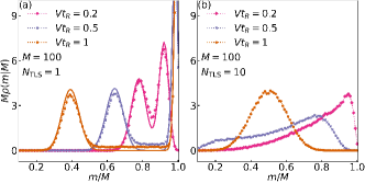
Figure 3: Nonergodic behavior for a different strength of the qubit to TLSs coupling. The results refer to $M=100$. (a) Coupling to a single TLS, $Wt_{R}=10^{3}$. Solid lines show the static limit, Eq. (I). (b) Coupling to 10 TLSs with the same switching rates as in Fig. 2.

Figure 3 shows the effect of the strength of the coupling to the TLSs for an intermediate number of measurements $M=100$. Panel (a) shows a profoundly double-peaked distribution for a single TLS, in excellent agreement with the static-limit (I). As expected, the distance between the peaks increases with the increasing coupling. For 10 TLSs, as seen in panel (b), the distribution is broad and strongly asymmetric. Both its shape and the position of the maximum sensitively depend on the coupling. It is important that the coupling parameter $Vt_{R}$ can be changed in the experiment by varying $t_{R}$, which helps pointing to the mechanism of the noise. We note the distinction from direct measurements of qubit frequency as a function of time [2, 5, 20], which is efficient for still much slower noise.

Discussion. To reach ergodic limit, a system of 10 TLSs has to visit its $2^{10}$ states. The needed time is a property of the TLSs themselves. However, the results of the measurements can approach quasi-ergodic limit, except for the far tail of the outcomes distribution, over a shorter time. This time depends on how the measurements are done. In our setup, the noise is measured by the qubit, and then the results are read through Ramsey measurements. An important parameter is the qubit-to-TLSs coupling, which we chose to be the same for all TLSs to avoid any bias. Unexpectedly, there is another important parameter, the phase $\phi_{R}$.

The effect of $\phi_{R}$ on the convergence to the ergodic limit is not obvious in advance. It comes through the dependence on $\phi_{R}$ of the centered correlator $\tilde{r}_{2}(k)$ of the measurement outcomes. For weak coupling to slowly switching TLSs, $V^{(n)}t_{R}\ll 1$ and $W^{(n)}t_{R}\ll 1$, and for small $\phi_{R}$ this correlator is small. Moreover, it falls off with the increasing $k$ much faster than for $\phi_{R}=\mathcal{O}(1)$ [48]. This indicates a reduced role of the noise correlations for small $\phi_{R}$. Respectively, the ergodic limit is reached must faster with the increasing $M$.

Conclusions We studied the distribution of the outcomes of periodically repeated Ramsey measurements with the sequence length $Mt_{\mathrm{cyc}}$ shorter than needed to approach the ergodic limit. Such distribution proves to provide an alternative, and sensitive, means of characterizing qubit frequency noise with a long correlation time. The analytical results and simulations show that, for non-Gaussian noise, in particular the noise from TLSs, the distribution can display a characteristic fine structure. Even where there is no fine structure, the form of the distribution and its evolution with the sequence length are noise-specific.

The results show that the way the system approaches the ergodic limit with the increasing number of quantum measurements depends not only on the noise source, but also on the character and parameters of the measurement. These parameters are not necessarily known in advance. Their effect can be strong and depends on the noise source. Measurement outcomes can practically approach the ergodic limit well before the noise source approaches this limit.

FW and MID acknowledge partial support from NASA Academic Mission Services, Contract No. NNA16BD14C, and from Google under NASA-Google SAA2-403512.

References

- Nakamura et al. [2002] Y. Nakamura, Yu. A. Pashkin, T. Yamamoto, and J. S. Tsai, Charge Echo in a Cooper-Pair Box, Phys. Rev. Lett. 88, 047901 (2002).
- Bialczak et al. [2007] R. C. Bialczak, R. McDermott, M. Ansmann, M. Hofheinz, N. Katz, E. Lucero, M. Neeley, A. D. O’Connell, H. Wang, A. N. Cleland, and J. M. Martinis, 1/f Flux Noise in Josephson Phase Qubits, Phys. Rev. Lett. 99, 187006 (2007).
- Álvarez and Suter [2011] G. A. Álvarez and D. Suter, Measuring the Spectrum of Colored Noise by Dynamical Decoupling, Phys. Rev. Lett. 107, 230501 (2011).
- Bylander et al. [2011] J. Bylander, S. Gustavsson, F. Yan, F. Yoshihara, K. Harrabi, G. Fitch, D. G. Cory, Y. Nakamura, J.-S. Tsai, and W. D. Oliver, Noise spectroscopy through dynamical decoupling with a superconducting flux qubit, Nat. Phys. 7, 565 (2011).
- Sank et al. [2012] D. Sank, R. Barends, R. C. Bialczak, Y. Chen, J. Kelly, M. Lenander, E. Lucero, M. Mariantoni, A. Megrant, M. Neeley, P. J. J. O’Malley, A. Vainsencher, H. Wang, J. Wenner, T. C. White, T. Yamamoto, Y. Yin, A. N. Cleland, and J. M. Martinis, Flux Noise Probed with Real Time Qubit Tomography in a Josephson Phase Qubit, Phys. Rev. Lett. 109, 067001 (2012).
- Yan et al. [2012] F. Yan, J. Bylander, S. Gustavsson, F. Yoshihara, K. Harrabi, D. G. Cory, T. P. Orlando, Y. Nakamura, J.-S. Tsai, and W. D. Oliver, Spectroscopy of low-frequency noise and its temperature dependence in a superconducting qubit, Phys. Rev. B 85, 174521 (2012).
- Young and Whaley [2012] K. C. Young and K. B. Whaley, Qubits as spectrometers of dephasing noise, Phys. Rev. A 86, 012314 (2012).
- Paz-Silva and Viola [2014] G. A. Paz-Silva and L. Viola, General Transfer-Function Approach to Noise Filtering in Open-Loop Quantum Control, Phys. Rev. Lett. 113, 250501 (2014).
- Yoshihara et al. [2014] F. Yoshihara, Y. Nakamura, F. Yan, S. Gustavsson, J. Bylander, W. D. Oliver, and J.-S. Tsai, Flux qubit noise spectroscopy using Rabi oscillations under strong driving conditions, Phys. Rev. B 89, 020503 (2014).
- Kim et al. [2015] M. Kim, H. J. Mamin, M. H. Sherwood, K. Ohno, D. D. Awschalom, and D. Rugar, Decoherence of Near-Surface Nitrogen-Vacancy Centers Due to Electric Field Noise, Phys. Rev. Lett. 115, 087602 (2015).
- Brownnutt et al. [2015] M. Brownnutt, M. Kumph, P. Rabl, and R. Blatt, Ion-trap measurements of electric-field noise near surfaces, Rev. Mod. Phys. 87, 1419 (2015).
- O’Malley et al. [2015] P. J. J. O’Malley, J. Kelly, R. Barends, B. Campbell, Y. Chen, Z. Chen, B. Chiaro, A. Dunsworth, A. G. Fowler, I.-C. Hoi, E. Jeffrey, A. Megrant, J. Mutus, C. Neill, C. Quintana, P. Roushan, D. Sank, A. Vainsencher, J. Wenner, T. C. White, A. N. Korotkov, A. N. Cleland, and J. M. Martinis, Qubit Metrology of Ultralow Phase Noise Using Randomized Benchmarking, Phys. Rev. Applied 3, 044009 (2015).
- Yan et al. [2016] F. Yan, S. Gustavsson, A. Kamal, J. Birenbaum, A. P. Sears, D. Hover, T. J. Gudmundsen, D. Rosenberg, G. Samach, S. Weber, J. L. Yoder, T. P. Orlando, J. Clarke, A. J. Kerman, and W. D. Oliver, The flux qubit revisited to enhance coherence and reproducibility, Nat Commun 7, 1 (2016).
- Myers et al. [2017] B. A. Myers, A. Ariyaratne, and A. C. B. Jayich, Double-Quantum Spin-Relaxation Limits to Coherence of Near-Surface Nitrogen-Vacancy Centers, Phys. Rev. Lett. 118, 197201 (2017).
- Quintana et al. [2017] C. M. Quintana, Y. Chen, D. Sank, A. G. Petukhov, T. C. White, D. Kafri, B. Chiaro, A. Megrant, R. Barends, B. Campbell, Z. Chen, A. Dunsworth, A. G. Fowler, R. Graff, E. Jeffrey, J. Kelly, E. Lucero, J. Y. Mutus, M. Neeley, C. Neill, P. J. J. O’Malley, P. Roushan, A. Shabani, V. N. Smelyanskiy, A. Vainsencher, J. Wenner, H. Neven, and J. M. Martinis, Observation of Classical-Quantum Crossover of $1/f$ Flux Noise and Its Paramagnetic Temperature Dependence, Phys. Rev. Lett. 118, 057702 (2017).
- Paz-Silva et al. [2017] G. A. Paz-Silva, L. M. Norris, and L. Viola, Multiqubit spectroscopy of Gaussian quantum noise, Phys. Rev. A 95, 022121 (2017).
- Ferrie et al. [2018] C. Ferrie, C. Granade, G. Paz-Silva, and H. M. Wiseman, Bayesian quantum noise spectroscopy, New J. Phys. 20, 123005 (2018).
- Noel et al. [2019] C. Noel, M. Berlin-Udi, C. Matthiesen, J. Yu, Y. Zhou, V. Lordi, and H. Häffner, Electric-field noise from thermally activated fluctuators in a surface ion trap, Phys. Rev. A 99, 063427 (2019).
- von Lüpke et al. [2020] U. von Lüpke, F. Beaudoin, L. M. Norris, Y. Sung, R. Winik, J. Y. Qiu, M. Kjaergaard, D. Kim, J. Yoder, S. Gustavsson, L. Viola, and W. D. Oliver, Two-Qubit Spectroscopy of Spatiotemporally Correlated Quantum Noise in Superconducting Qubits, PRX Quantum 1, 010305 (2020).
- Proctor et al. [2020] T. Proctor, M. Revelle, E. Nielsen, K. Rudinger, D. Lobser, P. Maunz, R. Blume-Kohout, and K. Young, Detecting and tracking drift in quantum information processors, Nat Commun 11, 5396 (2020).
- Wolfowicz et al. [2021] G. Wolfowicz, F. J. Heremans, C. P. Anderson, S. Kanai, H. Seo, A. Gali, G. Galli, and D. D. Awschalom, Qubit guidelines for solid-state spin defects, Nat. Rev. Mater. 6, 906 (2021), comment: 40 pages, 7 figures, 259 references.
- Wang and Clerk [2021] Y.-X. Wang and A. A. Clerk, Intrinsic and induced quantum quenches for enhancing qubit-based quantum noise spectroscopy, Nat Commun 12, 6528 (2021).
- Burgardt et al. [2023] S. Burgardt, S. B. Jäger, J. Feß, S. Hiebel, I. Schneider, and A. Widera, Measuring the environment of a Cs qubit with dynamical decoupling sequences (2023), arXiv:2303.06983 .
- Li et al. [2013] F. Li, A. Saxena, D. Smith, and N. A. Sinitsyn, Higher-order spin noise statistics, New J. Phys. 15, 113038 (2013).
- Ramon [2015] G. Ramon, Non-Gaussian signatures and collective effects in charge noise affecting a dynamically decoupled qubit, Phys. Rev. B 92, 155422 (2015).
- Norris et al. [2016] L. M. Norris, G. A. Paz-Silva, and L. Viola, Qubit Noise Spectroscopy for Non-Gaussian Dephasing Environments, Phys. Rev. Lett. 116, 150503 (2016).
- Sinitsyn and Pershin [2016] N. A. Sinitsyn and Y. V. Pershin, The theory of spin noise spectroscopy: A review, Rep. Prog. Phys. 79, 106501 (2016).
- Szańkowski et al. [2017] P. Szańkowski, G. Ramon, J. Krzywda, D. Kwiatkowski, and L Cywiński, Environmental noise spectroscopy with qubits subjected to dynamical decoupling, J. Phys.: Condens. Matter 29, 333001 (2017).
- Sung et al. [2019] Y. Sung, F. Beaudoin, L. M. Norris, F. Yan, D. K. Kim, J. Y. Qiu, U. von Lüpke, J. L. Yoder, T. P. Orlando, S. Gustavsson, L. Viola, and W. D. Oliver, Non-Gaussian noise spectroscopy with a superconducting qubit sensor, Nat. Commun. 10, 3715 (2019).
- Ramon [2019] G. Ramon, Trispectrum reconstruction of non-Gaussian noise, Phys. Rev. B 100, 161302(R) (2019).
- Sakuldee and Cywiński [2020] F. Sakuldee and Ł. Cywiński, Relationship between subjecting the qubit to dynamical decoupling and to a sequence of projective measurements, Phys. Rev. A 101, 042329 (2020).
- Wang and Clerk [2020] Y.-X. Wang and A. A. Clerk, Spectral characterization of non-Gaussian quantum noise: Keldysh approach and application to photon shot noise, Phys. Rev. Res. 2, 033196 (2020).
- You et al. [2021] X. You, A. A. Clerk, and J. Koch, Positive- and negative-frequency noise from an ensemble of two-level fluctuators, Phys Rev Res. 3, 013045 (2021), arxiv:2005.03591 .
- Paladino et al. [2002] E. Paladino, L. Faoro, G. Falci, and R. Fazio, Decoherence and 1/f Noise in Josephson Qubits, Phys. Rev. Lett. 88, 228304 (2002).
- Galperin et al. [2004] Y. M. Galperin, B. L. Altshuler, and D. V. Shantsev, Low-frequency noise as a source of dephasing of a qubit, in Fundamental Problems of Mesoscopic Physics, edited by I. V. Lerner (Kluwer Academic Publishing, The Netherlands, 2004) pp. 141–165, comment: 18 pages, 8 figures, Proc. of NATO/Euresco Conf. "Fundamental Problems of Mesoscopic Physics: Interactions and Decoherence", Granada, Spain, Sept.2003.
- Faoro and Viola [2004] L. Faoro and L. Viola, Dynamical Suppression of 1/f Noise Processes in Qubit Systems, Phys. Rev. Lett. 92, 117905 (2004).
- Galperin et al. [2006] Y. M. Galperin, B. L. Altshuler, J. Bergli, and D. V. Shantsev, Non-Gaussian Low-Frequency Noise as a Source of Qubit Decoherence, Phys. Rev. Lett. 96, 097009 (2006).
- Paladino et al. [2014] E. Paladino, Y. M. Galperin, G. Falci, and B. L. Altshuler, 1/f noise: Implications for solid-state quantum information, Rev. Mod. Phys. 86, 361 (2014).
- Müller et al. [2019] C. Müller, J. H. Cole, and J. Lisenfeld, Towards understanding two-level-systems in amorphous solids: Insights from quantum circuits, Rep. Prog. Phys. 82, 124501 (2019).
- Huang et al. [2022] Z. Huang, X. You, U. Alyanak, A. Romanenko, A. Grassellino, and S. Zhu, High-Order Qubit Dephasing at Sweet Spots by Non-Gaussian Fluctuators: Symmetry Breaking and Floquet Protection (2022), arxiv:2206.02827 [quant-ph] .
- Fink and Bluhm [2013] T. Fink and H. Bluhm, Noise Spectroscopy Using Correlations of Single-Shot Qubit Readout, Phys. Rev. Lett. 110, 010403 (2013).
- Nielsen and Chuang [2011] M. A. Nielsen and I. L. Chuang, Quantum Computation and Quantum Information: 10th Anniversary Edition, 1st ed. (Cambridge University Press, Cambridge ; New York, 2011).
- Van Kampen [2007] N. G. Van Kampen, Stochastic Processes in Physics and Chemistry, 3rd ed. (Elsevier, Amsterdam, 2007).
- Anderson et al. [1972] P. W. Anderson, B. I. Halperin, and C. M. Varma, Anomalous low-temperature thermal properties of glasses and spin glasses, Philos. Mag. J. Theor. Exp. Appl. Phys. 25, 1 (1972).
- Phillips [1972] W. A. Phillips, Tunneling states in amorphous solids, J Low Temp Phys 7, 351 (1972).
- Phillips [1987] W. A. Phillips, Two-Level States in Glasses, Rep. Prog. Phys. 50, 1657 (1987).
- Ithier et al. [2005] G. Ithier, E. Collin, P. Joyez, P. J. Meeson, D. Vion, D. Esteve, F. Chiarello, A. Shnirman, Y. Makhlin, J. Schriefl, and G. Schön, Decoherence in a superconducting quantum bit circuit, Phys. Rev. B 72, 134519 (2005).
- Note [1] See Supplemental Material for more results on , including the fine structure, the effect of asymmetric TLSs, and the transition to the ergodic limit.