SPIRiT-Diffusion: Self-Consistency Driven Diffusion Model for Accelerated MRI

Abstract

Diffusion models are a leading method for image generation and have been successfully applied in magnetic resonance imaging (MRI) reconstruction. Current diffusion-based reconstruction methods rely on coil sensitivity maps (CSM) to reconstruct multi-coil data. However, it is difficult to accurately estimate CSMs in practice use, resulting in degradation of the reconstruction quality. To address this issue, we propose a self-consistency-driven diffusion model inspired by the iterative self-consistent parallel imaging (SPIRiT), namely SPIRiT-Diffusion. Specifically, the iterative solver of the self-consistent term in SPIRiT is utilized to design a novel stochastic differential equation (SDE) for diffusion process. Then k-space data can be interpolated directly during the reverse diffusion process, instead of using CSM to separate and combine individual coil images. This method indicates that the optimization model can be used to design SDE in diffusion models, driving the diffusion process strongly conforming with the physics involved in the optimization model, dubbed model-driven diffusion. The proposed SPIRiT-Diffusion method was evaluated on a 3D joint Intracranial and Carotid Vessel Wall imaging dataset. The results demonstrate that it outperforms the CSM-based reconstruction methods, and achieves high reconstruction quality at a high acceleration rate of 10.

Diffusion Models, Parallel Imaging, K-Space Interpolation, Inverse Problem

1 Introduction

Magnetic resonance imaging (MRI) is widely used in clinical and research domains. However, its long acquisition time is still a major limitation, resulting in trade-offs between spatial and temporal resolution or coverage. As a result, there is a growing interest in reconstructing high-quality MR images from a limited amount of $k$-space data to accelerate acquisitions. The advances of compressed sensing (CS)[1, 2, 3, 4, 5, 6] and deep learning (DL)[7, 8, 9, 10, 11] have made substantial progress in MR reconstruction field over the past few decades. They leverage image prior information to create hand-crafted or learnable regularizations, which are combined with a data consistency term to solve the ill-posed inverse problem of MR reconstruction.

Most recently, score-based diffusion models[12, 13, 14, 15] have emerged as a powerful deep generative prior in MR reconstruction[16, 17, 18]. These approaches rely on forward and reverse stochastic differential equations (SDEs) to encode and decode (generate) images. The forward SDE comprises a drift term that represents the deterministic trend of the forward process, and a diffusion term that introduces random fluctuations. For example, the drift term in Variance Preserving (VP)-SDE[14] is a deterministic trend of energy reduction linearly, representing that the mean of the image signal decays to zero deterministically. The reverse SDE is derived from the forward one, leveraging the score function of the marginal probability densities. Image reconstruction is achieved through the reverse process based on the reverse SDE, using acquired $k$-space data as guidance. Notably, score-based MR reconstruction learns the data distribution instead of end-to-end mapping between $k$-space data and images. Therefore it enables unsupervised learning and facilitates the adaptation to out-of-distribution data. The method has yielded promising results, as reported in the literature.

In practical use, all reconstruction methods need to be extended to multi-coil forms, since modern MR systems typically acquire multi-coil data simultaneously using multiple receiver coils. A commonly employed strategy is to incorporate the spatial sensitivity maps of individual coils into the reconstruction model as weighting functions of coil images. Specifically, an image is first recovered via compressed sensing or a neural network. Then it multiplies each coil sensitivity map (CSM) to obtain the coil image, respectively, which will be used in the data consistency term. These two steps perform iteratively until convergence. However, it is difficult to accurately measure the CSMs, especially when FOV limited [19] or existing rapid field variations. Even small errors in coil sensitivities can lead to inconsistency between coil images and acquired $k$-space data, resulting in artifacts in the reconstructed image. On the other hand, direct interpolation of missing $k$-space data can avoid the difficulties associated with CSM estimation, such as parallel imaging (PI) methods in $k$-space, GRAPPA[20] uses shift-invariant convolutional kernels to estimate missing $k$-space data, and is more robust to inaccurate coil sensitivity estimation relative to SENSE. SPIRiT[21] generalizes the GRAPPA method by enforcing self-consistency with the calibration and acquisition data, resulting in more accurate reconstruction and better noise behavior.

From an optimization perspective, the iterative algorithm for solving the SPIRiT inverse problem can be treated as the Euler discrete form of some SDEs. Inspired by this, we propose a novel diffusion-based MR reconstruction method that employs the self-consistent term of SPIRiT as the drift coefficient in the SDE. Furthermore, coil sensitivity maps are integrated into the diffusion coefficient of this SDE to calculate the mean and variance of the perturbation kernel accurately. This method no longer uses the explicit coil sensitivity for data consistency and therefore is robust to inaccurate sensitivity estimation. More importantly, it can achieve a high acceleration with more tiny structures preserved by exploiting both correlations among multi-coil data and the prior from learned data distributions. Because this method draws inspiration from SPIRiT in the sense of self-consistency, we referred to it as SPIRiT-Diffusion in this manuscript.

1.1 Contributions

1. We developed a novel paradigm for SDE design in the diffusion model, dubbed model-driven diffusion. That is, the drift term of SDE can be designed based on the iteration solution of an optimization model, driving the diffusion process conforming with the physics involved in the optimization model.

2. We proposed a new diffusion-based MR reconstruction model with the SDE derived from the self-consistency term of SPIRiT, addressing the issues from inaccurate coil sensitivity estimation.

This paper is organized as follows. Section 2 introduces the background; Section 3 describes the related works; Section 4 presents the proposed method and implementation details; Section 5 provides the experimental results. The discussion and conclusion are in Sections 6 and 7, respectively.

2 Background

2.1 SPIRiT Method

The forward model for MR reconstruction can be expressed as follows:

$$\mathbf{y}=\mathbf{A}\mathbf{x}+\mathbf{n},$$ (1)

where $\mathbf{x}$ is the image to be reconstructed, $\mathbf{y}$ is the undersampled $k$-space data, $\mathbf{n}$ is the Gaussian noise, and $\mathbf{A}$ is the encoding matrix, see Table 1 for details of the meaning.

The SPIRiT method is a self-consistent method for coil-by-coil reconstruction, which can be used for data from arbitrary $k$-space sampling patterns. SPIRiT formulates the MR reconstruction as the following optimization problem:

$$\underset{\mathbf{\hat{x}}}{\arg\min}\|\mathbf{G\hat{x}}-\mathbf{\hat{x}}\|_{2}^{2},~{}~{}~{}s.t.~{}\|\mathbf{A}\mathbf{x}-\mathbf{y}\|_{2}^{2}\leq\epsilon,$$ (2)

where $\epsilon$ is the parameter to control data consistency. The first term is the self-consistency constraint, and the second one is the consistency with the data acquisition. The kernel $\mathbf{G}$ convolves the entire undersampling $k$-space to interpolate the missing $k$-space data. If $\mathbf{\hat{x}}$ is the true solution, the point synthesized from its neighborhood is equal to itself, i.e. $\mathbf{G\hat{x}}=\mathbf{\hat{x}}$.

Table 1: Meaning of mathematical symbols in background and methods.

Symbol	Symbol Meaning
$\mathbb{F}$	Fourier operator
$\mathbf{x}$	MR image
$\mathbf{\hat{x}}$	$k$-space data, $\mathbf{\hat{x}}=\mathbb{F}(\mathbf{x})$
$\mathbf{M}$	undersampling operator
$\mathbf{I}$	identity matrix
$\mathbf{S}$	coil sensitivity maps, $\mathbf{S}=[\mathbf{s}_{1},\mathbf{s}_{2},...,\mathbf{s}_{m}]$, $\mathbf{S^{*}S}=\mathbf{I}$
$\mathbf{A}$	encoding matrix, $\mathbf{A}=\mathbf{M}\mathbb{F}\mathbf{S}$
$\mathbf{y}$	undersampled $k$-space data, $\mathbf{y}=\mathbf{Ax}$
$\mathbf{G}$	kernel in SPIRiT[21], $\mathbf{\hat{x}}=\mathbf{G\hat{x}}$
$\Psi$	$\Psi(\cdot)=\mathbb{F}^{-1}(\mathbf{G}-\mathbf{I})^{H}(\mathbf{G}-\mathbf{I})\mathbb{F}(\cdot)$

2.2 Score-Based Diffusion Model

Score-based diffusion model is a framework of diffusion generative models. It perturbs data by injecting different scales of Gaussian noise to gradually transform the data distribution to Gaussian distribution, and then generates samples from the Gaussian noise according to the corresponding reverse process. The diffusion process $\{\mathbf{x}(t)\}_{t=0}^{T}$ can be seen as the solution of the forward SDE as follows:

$$\mathrm{d}\mathbf{x}=\mathbf{f}(\mathbf{x},t)\mathrm{d}t+g(t)\mathrm{d}\mathbf{w},$$ (3)

where $t$ is the continuous time variable, $t\in[0,T]$, $\mathbf{x}(0)\sim p_{0}=p_{data}$, $\mathbf{x}(T)\sim p_{T}$ and $p_{T}$ is a prior distribution, typically using Gaussian distribution. $\mathbf{f}$ and $g$ are the drift and diffusion coefficients of $\mathbf{x}(t)$, and $\mathbf{w}$ is the standard Wiener process.

The reverse-time SDE of Eq. (3) is:

$$\mathrm{d}\mathbf{x}=\left[\mathbf{f}(\mathbf{x},t)-g(t)^{2}\nabla_{\mathbf{x}}\log p_{t}(\mathbf{x})\right]\mathrm{d}t+g(t)\mathrm{d}\mathbf{\bar{w}},$$ (4)

where $\mathbf{\bar{w}}$ is the standard Wiener process for the time from $T$ to $0$. The score function $\nabla_{\mathbf{x}}\log p_{t}(\mathbf{x})$ is approximated by the score model $\mathbf{s}_{\boldsymbol{\theta}}$ trained by

$$\boldsymbol{\theta}^{*}=\underset{\boldsymbol{\theta}}{\arg\min}\mathbb{E}_{t}\Big{\{}\lambda(t)\mathbb{E}_{\mathbf{x}(0)}\mathbb{E}_{\mathbf{x}(t)\mid\mathbf{x}(0)}\big{[}\big{\|}\mathbf{s}_{\boldsymbol{\theta}}(\mathbf{x}(t),t)\\ -\nabla_{\mathbf{x}(t)}\log p_{0t}(\mathbf{x}(t)\mid\mathbf{x}(0))\big{\|}_{2}^{2}\big{]}\Big{\}},$$ (5)

where $p_{0t}(\mathbf{x}(t)\mid\mathbf{x}(0))$ is the perturbation kernel and can be derived from the forward diffusion process. Once the score model $\mathbf{s}_{\boldsymbol{\theta}}$ is trained, we can generate samples through reverse-time SDE.

3 Related Works

3.1 K-Space PI Methods using DL

There are several deep learning reconstruction methods based on $k$-space interpolation, such as RAKI[22], LORAKI[23], DL-SPIRiT[24], $k$-space DL[25], and Deep-SLR[26].

RAKI is based on GRAPPA method. It trains a neural network using autocalibration signal (ACS) data to learn the GRAPPA kernel instead of solving the linear function. LORAKI is an extension of RAKI for Autocalibrated LORAKS method[27], which can be treated as a GRAPPA method with substantially more constraints. LORAKI uses a recurrent neural network to precisely compute the calibration kernel for interpolating the missing $k$-space data. DL-SPIRiT is based on the unrolling method that unrolls the iterative solution of L1-SPIRiT method[28, 29] into a neural network. The employed algorithm is the projection onto convex sets (POCS) method.

Another strategy to directly interpolate $k$-space data is the annihilating filter-based low-rank Hankel matrix approach (ALOHA), which estimates annihilation relations using low-rank matrix complementation. Based on the principle of ALOHA, Ye et al.[25] incorporated convolutional neural networks (CNNs) and Hankel matrix decomposition to interpolate missing data in $k$-space.

A major issue in ALOHA is SLR matrix completion has high computational complexity because they learn all parameters for a set of linear filters from the dataset itself. To overcome this issue, Jacob et al.[26] proposed Deep-SLR method that uses CNNs to represent the filter parameters using the convolutional kernel, avoiding the SLR matrix completion.

3.2 Score-Based Diffusion Model for MR Reconstruction

Score-based diffusion model has been applied to MR reconstruction and has shown promising results. Jalal et al.[18] was the first one to employ this method. They trained the score function using the fastMRI dataset and subsequently employed posterior sampling with Langevin to generate high-quality reconstructed data. The controllable generation is achieved through the reverse diffusion process with the posterior distribution $\nabla_{\mathbf{x}}\log p_{t}(\mathbf{x}\mid\mathbf{y})$:

$$\nabla_{\mathbf{x}}\log p_{t}(\mathbf{x}(t)\mid\mathbf{y}) =\nabla_{\mathbf{x}}\log p_{t}(\mathbf{x}(t))+\nabla_{\mathbf{x}}\log p_{t}(\mathbf{y}\mid\mathbf{x}(t))$$ (6)

$$\approx\mathbf{s}_{{\boldsymbol{\theta}}^{*}}(\mathbf{x}(t),t)+\nabla_{\mathbf{x}}\log p_{t}(\mathbf{y}\mid\mathbf{x}(t))$$

$$=\mathbf{s}_{{\boldsymbol{\theta}}^{*}}(\mathbf{x}(t),t)+\frac{\mathbf{A}^{H}(\mathbf{y}-\mathbf{A}\mathbf{x}(t))}{\sigma^{2}_{\epsilon}},$$

where $\mathbf{y}$ is the undersampled $k$-space data and $\mathbf{x}$ is the desired MR image.

Using a similar approach, Song et al. utilized the score-based diffusion model to solve the inverse problems in both MRI and CT[16]. But they just tested on single-coil data. For multi-coil scenarios, Chung et al.[17] proposed two approaches: one to integrate the CSMs in the encoding matrix $\mathbf{A}$. The other was to reconstruct coil images individually and combine the reconstructed images via the sum of squares method.

4 Methodology

In this section, we’ll introduce the SPIRiT-Diffusion method, followed by a description of score model training and implementation details.

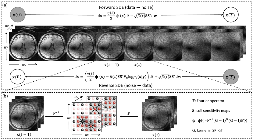
Figure 1: The framework of SPIRiT-Diffusion. (a) In the forward process, self-consistency noise at different scales is gradually injected into the multi-coil images. (b) The detailed reverse process from $t$ to $t-1$: first, transform $\mathbf{x}(t)$ to $k$-space domain; then fill in the missing points; and finally, transform k-space data back to the image domain.

4.1 SPIRiT-Diffusion Model

4.1.1 Forward SDE

Eq. (2) in the SPIRiT method can be solved using the gradient descent algorithm with the following iterative solution:

$$\mathbf{x}_{k}=\mathbf{x}_{k+1}+\eta_{k+1}\mathbb{F}^{-1}((\mathbf{G}-\mathbf{I})^{H}(\mathbf{G}-\mathbf{I})\mathbb{F}(\mathbf{x}_{k+1}))+\\ \lambda_{k+1}\mathbf{A}^{H}(\mathbf{Ax_{k+1}}-\mathbf{y})\quad k=T-1,\cdots,0,$$ (7)

where $\eta_{k}$ and $\lambda_{k}$ denote the stepsize. Suppose Eq. (7) is viewed roughly as the discrete form of the reverse diffusion process conditioned on $\mathbf{Ax}-\mathbf{y}=\mathbf{n}$. The gradient of the self-consistency term can be treated as the drift coefficient $\mathbf{f}(\mathbf{x},t)$ of the diffusion process. A new SDE can be derived:

$$\mathrm{d}\mathbf{x}=\frac{\eta(t)}{2}\Psi(\mathbf{x})\mathrm{d}t+\sqrt{\beta(t)}\mathrm{d}\mathbf{w},$$ (8)

where $\Psi(\cdot)=\mathbb{F}^{-1}(\mathbf{G}-\mathbf{I})^{H}(\mathbf{G}-\mathbf{I})\mathbb{F}(\cdot)$, $\beta(t)$ is the parameter to control the noise level, and $\eta(t)$ is the serialization of $\eta_{k}$. The perturbation kernel can be derived by Eqs. 5.50 and 5.51 in [30] as:

$$p_{0t}(\mathbf{x}(t)\mid\mathbf{x}(0))=\mathcal{N}\big{(}\mathbf{x}(t);e^{\frac{1}{2}\int_{0}^{t}\eta(s)\Psi ds}\mathbf{x}(0),\\ \frac{1}{2}\int_{0}^{t}\beta(\tau)e^{\int_{\tau}^{t}\eta(s)ds}d\tau e^{2\Psi}\big{)},\quad t\in[0,1].$$ (9)

Since $\mathbf{\Psi}(\mathbf{x}(0))=0$, the mean $\boldsymbol{\mu}$ can be calculated using Taylor expansion as follows:

$$\boldsymbol{\mu}= e^{\frac{1}{2}\int_{0}^{t}\eta(s)\Psi ds}\mathbf{x}(0)$$ (10)

$$= \Big{(}\mathbf{I}+\frac{1}{2}\int_{0}^{t}\eta(s)\Psi ds+\frac{1}{2!}(\frac{1}{2}\int_{0}^{t}\eta(s)\Psi ds)^{2}+$$

$$o((\frac{1}{2}\int_{0}^{t}\eta(s)\Psi ds)^{3})\Big{)}\mathbf{x}(0)$$

$$= \mathbf{x}(0).$$

But for the covariance $\boldsymbol{\Sigma}$, the noise dose not have the property of self-consistency and the Taylor expansion of $e^{2\Psi}$ is computationally intolerable and time-consuming. We have tried using the first-order Taylor series as an approximation. But the gap between this approximation and the real one is too large to learn the true data distribution, and experiments showed poor performance.

To solve this issue, we introduce the coil redundancy to the diffusion coefficient, enforcing the self-consistency property to the Gaussian noise during the diffusion process, i.e. $\mathbf{GS}\mathbf{S}^{*}(\mathbf{z})=\mathbf{z}$ which implies $\mathbf{\Psi}(\mathbf{S}\mathbf{S}^{*}\mathbf{z})=0$, where $\mathbf{z}\sim\mathcal{N}(\mathbf{0},\mathbf{I})$ and $\mathbf{S}$ is the CSM. The corresponding forward SPIRiT-Diffusion process is:

$$\mathrm{d}\mathbf{x}=\frac{\eta(t)}{2}\Psi(\mathbf{x})\mathrm{d}t+\sqrt{\beta(t)}\mathbf{S}\mathbf{S}^{*}\mathrm{d}\mathbf{w}.$$ (11)

Then the perturbation kernel becomes:

$$p_{0t}(\mathbf{x}(t)\mid\mathbf{x}(0))=\mathcal{N}\big{(}\mathbf{x}(t);\mathbf{x}(0),\\ \frac{1}{2}\int_{0}^{t}\beta(\tau)e^{\int_{\tau}^{t}\eta(s)ds}d\tau e^{\Psi}\mathbf{S}\mathbf{S}^{*}[e^{\Psi}\mathbf{S}\mathbf{S}^{*}]^{*}\big{)},\quad t\in[0,1].$$ (12)

Let $\sigma=\sqrt{\frac{1}{2}\int_{0}^{t}\beta(\tau)e^{\int_{\tau}^{t}\eta(s)ds}d\tau}$, the covariance can be calculated as follows:

$$\boldsymbol{\Sigma^{\frac{1}{2}}}= \sigma e^{\Psi}\mathbf{S}\mathbf{S}^{*}(\cdot)$$ (13)

$$= \sigma(\mathbf{I}+\Psi+\frac{1}{2!}\Psi^{2}+o(\Psi^{3}))\mathbf{S}\mathbf{S}^{*}(\cdot)$$

$$= \sigma\mathbf{S}\mathbf{S}^{*}(\cdot).$$

The final expression of the perturbation kernel is

$$p_{0t}(\mathbf{x}(t)\mid\mathbf{x}(0))=\mathcal{N}\big{(}\mathbf{x}(t);\mathbf{x}(0),\sigma^{2}\mathbf{S}\mathbf{S}^{*}\big{)},\quad t\in[0,1].$$ (14)

4.1.2 Estimating Score Functions

Since CSM is integrated into the diffusion coefficient of the SPIRiT-Diffusion, it is infeasible to train the score model by estimating pure Gaussian noise. According to the perturbation kernel in Eq. (14), the loss function of the score model in SPIRiT-Diffusion is derived as (details in Appendix .1):

$$\boldsymbol{\theta}^{*}=\underset{\boldsymbol{\theta}}{\arg\min}\mathbb{E}_{t}\big{\{}\lambda(t)\mathbb{E}_{\mathbf{x}(0)}\mathbb{E}_{\mathbf{x}(t)\mid\mathbf{x}(0)}\big{[}\big{\|}\sigma\mathbf{S}^{*}\mathbf{s}_{\boldsymbol{\theta}}(\mathbf{x}(t),t)\\ +\mathbf{S}^{*}\mathbf{z}\big{\|}_{2}^{2}\big{]}\big{\}}.$$ (15)

4.1.3 Reverse SDE

After the score model is trained, MR images can be reconstructed by the conditional reverse SPIRiT-Diffusion process as:

$$\mathrm{d}\mathbf{x}=\Big{[}\frac{\eta(t)}{2}\Psi(\mathbf{x})-\beta(t)\mathbf{S}\mathbf{S}^{*}\nabla_{\mathbf{x}}\log p_{t}(\mathbf{x}\mid\mathbf{y})\Big{]}\mathrm{d}t\\ +\sqrt{\beta(t)}\mathbf{S}\mathbf{S}^{*}\mathrm{d}\mathbf{\bar{w}}.$$ (16)

The whole framework of SPIRiT-Diffusion is shown in Fig. 1, and the Predictor-Corrector method (PC Sampling) is used to generate MR images, as presented in Alg. 1.

Algorithm 1 PC Sampling (SPIRiT-Diffusion).

1:$\eta(t),\{\beta_{i}\}_{i=1}^{N},\sigma,\mathbf{S},\mathbf{y},\lambda_{1},\lambda_{2},r,N,\mathbf{M}$.

2:$\mathbf{x}_{N}\sim\mathcal{N}(\mathbf{0},(\sigma\mathbf{S}\mathbf{S}^{*})^{2})$

3:for $i=N-1$ to $0$ do

4:     $\mathbf{z}\sim\mathcal{N}(\mathbf{0},\mathbf{I})$

5:     $\mathbf{g}\leftarrow\mathbf{s}_{\boldsymbol{\theta^{*}}}\left(\mathbf{x}_{i+1},i+1\right)$

6:     $\mathbf{m}=\sum_{j=1}^{n}\mathbf{S}^{*}\mathbb{F}^{-1}\left(\mathbb{F}(\mathbf{S}\cdot\mathbf{x}_{i})\cdot\mathbf{M}-\mathbf{y}\right)$

7:     $\epsilon\leftarrow\lambda_{1}\left(\|\mathbf{g}\|_{2}/\|\mathbf{m}\|_{2}\right)$

8:     $\mathbf{x}_{i}\leftarrow\mathbf{x}_{i+1}+\frac{1}{2}\eta_{i+1}\Psi(\mathbf{x}_{i})+\beta_{i+1}\mathbf{SS}^{*}(\mathbf{g}-\epsilon\mathbf{m})+\sqrt{\beta_{i+1}}\mathbf{SS}^{*}(\mathbf{z})$

9:     for $k\leftarrow 1$ to $M$ do

10:         $\mathbf{z}\sim\mathcal{N}(\mathbf{0},\mathbf{I})$

11:         $\mathbf{g}\leftarrow\mathbf{s}_{\boldsymbol{\theta}^{*}}\left(\mathbf{x}_{i}^{k-1},i\right)$

12:         $\mathbf{m}=\sum_{j=1}^{n}\mathbf{S}^{*}\cdot\mathbb{F}^{-1}\left(\mathbb{F}(\mathbf{S}\cdot\mathbf{x}_{i}^{k})\mathbf{M}-\mathbf{y}\right)$

13:         $\epsilon_{1}\leftarrow 2\left(r\|\mathbf{z}\|_{2}/\|\mathbf{g}\|_{2}\right)^{2}$

14:         $\epsilon_{2}\leftarrow\lambda_{2}\left(\|\mathbf{g}\|_{2}/\|\mathbf{m}\|_{2}\right)$

15:         $\mathbf{x}_{i}^{k}\leftarrow\mathbf{x}_{i}^{k-1}+\frac{1}{2}\eta_{i+1}\Psi(\mathbf{x}_{i}^{k-1})+\epsilon_{1}\mathbf{SS}^{*}(\mathbf{g}-\epsilon_{2}\mathbf{m})+\sqrt{2\epsilon_{1}}\mathbf{SS}^{*}(\mathbf{z})$

16:     end for

17:     $\mathbf{x}_{i-1}^{0}\leftarrow\mathbf{x}_{i}^{M}$

18:end for

19:return ${\mathbf{x}}_{0}^{0}$

4.2 Implementation Details

The network structure of SPIRiT-Diffusion is the same as that of VE-SDE (ncsnpp). The exponential moving average (EMA) rate is set to $0.999$, $\beta_{max}=348$, $\beta_{min}=0.01$, and the batch size is set to 1. Unlike previous approaches that combine multi-coil data into a single channel for network training, SPIRiT-Diffusion directly inputs multi-coil images to the network. The complex MR data is split into real and imaginary components and concatenated before input into the network, resulting in an input tensor of size $nc\times 2\times nx\times ny$. $nc$ is the coil number, $2$ represents the concatenated real and imaginary parts of the data, and $nx$ and $ny$ represent the image size. The coil dimension is permuted to the batch size dimension to keep the convolution parameters of each channel consistent. The network is trained for 100 epochs in a computing environment using the torch1.13 library[31], cuda11.6 on an NVIDIA A100 Tensor Core GPU.

5 Experiments

5.1 Experimental setup

5.1.1 Datasets

We conducted experiments on a 3D joint Intracranial and Carotid Vessel Wall Imaging (VWI) dataset, including fully sample $k$-space data from 11 healthy volunteers and a prospectively 4.5-fold undersampled data from 1 stroke patient. The dataset was acquired using a 3T MR scanner (uMR 790, United Imaging Healthcare, China) with the combination of a 32-channel head coil and an 8-channel neck coil. The imaging parameters were: acquisition matrix = 384×318×240-256 (RO×PE1×PE2), FOV = 232×192×144-154 (HF×AP×LR) mm³, Acq. resolution = 0.6mm³ (isotropic), TR/TE = 800/135 ms, scan time of full sample = 20 to 22 minutes. Inverse Fourier transform was applied in the RO direction first, and then the 3D $k$-space data were split into 2D slices along the RO direction. Zero-padding of $k$-space data was applied in PE directions, resulting in the image size of $320\times 320$. Ten healthy volunteers were randomly selected as the training dataset, total of 3680 images. The remaining data from the healthy volunteer were used as test dataset I (300 images), and the data from the stroke patient were used as test dataset II (320 images).

5.1.2 Parameter Configuration

SPIRiT-Diffusion is compared with different types of reconstruction methods, including SPIRiT[21], DL-SPIRiT[24], ISTA-Net[32], and VE-SDE based on CSMs[17]. The deep learning-based methods were trained using identical training data. ISTA-Net and DL-SPIRiT underwent 50 epochs of training. All score-based SDEs methods underwent 500 epochs of training.

5.1.3 Performance Evaluation

Three metrics were used to evaluate the results quantitatively, including normalized mean square error (NMSE), the peak signal-to-noise ratio (PSNR), and the structural similarity index (SSIM)[33]. The metrics were calculated on the imaging region, removing the background.

5.2 Experimental Results

5.2.1 Retrospective Experiments

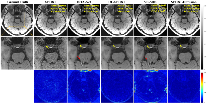
Figure 2: Reconstruction results of VWI data at 7.6-fold. The top row shows the ground truth and the reconstructions obtained using different methods. The second row shows an enlarged view of the ROI and the third row displays the error map of the reconstructions. The result of SPIRiT shows severe noise amplification. DL-SPIRiT can suppress noise but loses tiny structures. Aliasing artifacts appear on the images of ISTA-Net and VE-SDE. SPIRiT-Diffusion achieves good reconstruction quality.

Figure 3: Reconstruction results of VWI data at 10-fold. The top row shows the ground truth and the reconstructions obtained using different methods. The second row shows an enlarged view of the ROI and the third row displays the error map of the reconstructions. The vessel wall (yellow arrow) can be barely seen on the images using other compared reconstruction methods at such a high acceleration rate. SPIRiT-Diffusion can still achieve good reconstruction quality.

We retrospectively undersampled the test dataset I with 7.6- and 10-fold, respectively. Fig. 2 shows the reconstruction results of 7.6-fold undersampling. The result of SPIRiT shows severe noise amplification since it is based on the parallel imaging method. DL-SPIRiT can suppress noise but also loses tiny structures (yellow arrow), which is a common issue for DL-based reconstructions. The reconstruction quality of VE-SDE is poor, and artifacts can be easily seen in the image. This is because the estimated CSMs are inaccurate due to the FOV aliasing, especially at the image’s border. SPIRiT-Diffusion achieves good reconstruction quality with the highest quantitative metrics among compared methods.

Fig. 3 shows the results of 10-fold undersampling. SPIRiT-Diffusion can still achieve good reconstruction quality with quantitative metrics slightly degraded. The vessel wall (yellow arrow) can be barely seen on the images using other compared reconstruction methods at such a high acceleration rate. More aliasing artifacts appear on the images reconstructed by VE-SDE and ISTA-Net relative to 7.6-fold undersampling.

The average quantitative metrics of test dataset I are shown in Table 2. SPIRiT-Diffusion achieved the best NMSE and PSNR.

5.2.2 Prospective Experiments

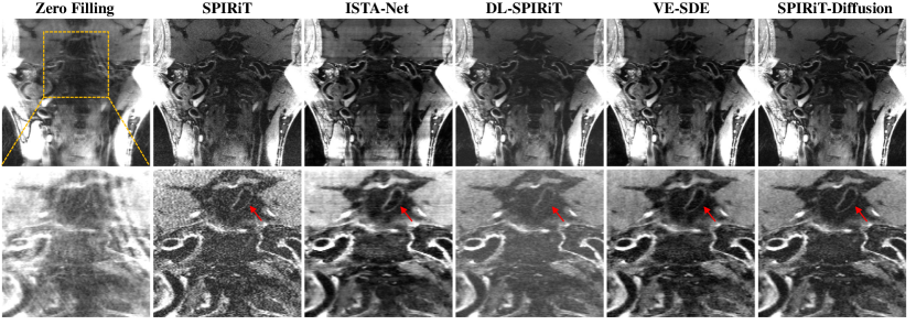
Figure 4: Prospective reconstruction results of VWI data at 4.5-fold. The top row shows the ground truth and the reconstructions obtained using different methods. The second row shows an enlarged view of the ROI indicated by the yellow box in the first row. The image of SPIRiT is a bit noisy. Aliasing artifacts appear on the images of ISTA-Net and VE-SDE. The result of DL-SPIRiT loses parts of the vessel wall. SPIRiT-Diffusion can suppress artifacts and noise well.

Fig. 4 shows the reconstruction results of the prospectively undersampled VWI data from the stroke patient at the coronal view. Similar conclusions can be drawn from the retrospective study. The image of SPIRiT is a bit noisy. Aliasing artifacts appear on the images of ISTA-Net and VE-SDE. Parts of the vessel wall were lost on the images of DL-SPIRiT. SPIRiT-Diffusion can suppress artifacts and noise well, and the vessel wall can be clearly seen in its image.

6 Discussion

This study has demonstrated that the self-consistency property of $k$-space data can be incorporated into an SDE to interpolate $k$-space in diffusion-based MR reconstruction. Based on this, the proposed SPIRiT-Diffusion method for coil-by-coil reconstruction avoids the issues induced by inaccurate coil sensitivity estimation. Since this method exploits both data distribution prior and the correlations among multi-coil data, it can reconstruct high-quality images at a high acceleration of 10-fold in 3D imaging. Even in the case the reconstruction failed by image domain methods such as ISTA-Net and VE-SDE, SPIRiT-Diffusion still can achieve a solution. We chose 3D VWI data for testing since 3D VWI has a large FOV coverage, and reduced FOV is typically employed to shorten the scan time. In this scenario, it is difficult to estimate CSMs accurately and can better verify that SPIRiT-Diffusion improves the robustness of inaccurate CSMs. In addition, we developed the model-driven diffusion that integrates a traditional optimization model into the diffusion model, making the diffusion process more conform to the constraints compared with pure data-driven diffusion.

6.1 The effect of CSM estimation methods

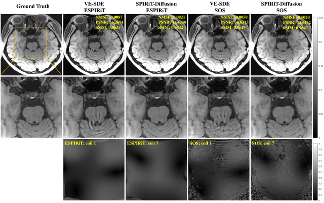
Figure 5: Reconstruction results of VWI data at 7.6-fold with the CSM estimated by different methods. The top row displays the ground truth and the reconstruction obtained using VE-SDE and SPIRiT-Diffusion (proposed method). The second row shows an enlarged view of the ROI and the third row displays the CSM estimated by ESPIRiT and SOS. The CSM variation has little effect on the performance of SPIRiT-Diffusion.

Table 2: The average quantitative metrics on the SIAT vessel wall imaging dataset at 7.6-fold and 10-fold.

AF	Methods	NMSE(*e-2)	PSNR (dB)	SSIM(*e-2)
7.6	SPIRiT	1.20 $\pm$ 1.64	38.68 $\pm$ 4.81	95.20 $\pm$ 4.05
	ISTA-Net	0.59 $\pm$ 0.41	41.02 $\pm$ 4.20	98.06 $\pm$ 1.66
	DL-SPIRiT	0.41 $\pm$ 0.27	42.35 $\pm$ 3.69	98.42 $\pm$ 1.23
	VE-SDE	0.80 $\pm$ 0.50	39.56 $\pm$ 3.95	97.44$\pm$ 1.92
	SPIRiT-Diffusion	0.38 $\pm$ 0.24	42.74 $\pm$ 3.79	98.35 $\pm$ 1.35
10	SPIRiT	2.06 $\pm$ 2.60	36.48 $\pm$ 4.98	92.99 $\pm$ 6.14
	ISTA-Net	0.90 $\pm$ 0.54	39.04 $\pm$ 3.95	97.48 $\pm$ 2.08
	DL-SPIRiT	0.62 $\pm$ 0.48	40.78 $\pm$ 3.95	97.95 $\pm$ 1.55
	VE-SDE	1.05 $\pm$ 0.72	38.40 $\pm$ 3.91	96.72 $\pm$ 2.50
	SPIRiT-Diffusion	0.58 $\pm$ 0.39	40.97 $\pm$ 3.66	97.99 $\pm$ 1.56

Table 3: Using the CSM estimated by different methods, the average quantitative metrics on the SIAT vessel wall imaging dataset at 7.6-fold.

Estimated	Methods	NMSE(*e-3)	PSNR (dB)	SSIM(*e-2)
ESPIRiT	VE-SDE	8.57 $\pm$ 5.69	37.56 $\pm$ 5.62	95.94 $\pm$ 3.85
ESPIRiT	SPIRiT-Diffusion	3.68 $\pm$ 2.29	41.14 $\pm$ 4.87	97.31 $\pm$ 2.63
SOS	VE-SDE	6.78 $\pm$ 3.54	38.25 $\pm$ 4.78	95.35 $\pm$ 4.24
SOS	SPIRiT-Diffusion	3.61 $\pm$ 2.04	41.17 $\pm$ 4.87	97.30 $\pm$ 2.64

There are several CSM estimation methods proposed that rely on different assumptions, such as adaptive CSM and ESPIRiT[19]. We tested the performance of SPIRiT-Diffusion with CSM estimated using different methods to verify that the variation of CSM has little effect on the reconstruction quality. Two CSM methods were adopted: one was a simple method that directly used the conjugate of the low-resolution ($48\times 48$ ACS region) coil images, as indicated in the sum-of-squares (SOS) method; the other was the ESPIRiT method assembled in bart[34], which is popularly used in MR reconstruction research. Fig. 5 shows the reconstructed results using SPIRiT-Diffusion and VE-SDE at 7.6-fold, along with the representative CSMs estimated. The reconstruction quality of VE-SDE relies on the CSM methods, while the images of SPIRiT-Diffusion are close when using different CSM estimation methods. The average quantitative metrics of test dataset I are shown in Table 3. This experiment verified that although CSM is integrated as a weighting function into the diffusion coefficient to reduce the computational complexity in calculating the perturbation kernel, its variation has little effect on the performance of SPIRiT-Diffusion.

6.2 The model-driven diffusion model

Physics plays an important role in MR imaging and is generally utilized to construct the optimization model for MR reconstruction. However, the conventional diffusion model is trained solely on image domain distributions and does not leverage these physics. To integrate imaging physics into diffusion models, we can roughly treat the iterative solution of an optimization model as the reverse diffusion process. That is, the iterative solution would correspond to the drift coefficient of the reverse-time SDE. In this scenario, the physics in any optimization model can be used to “drive” the diffusion process by designing the SDE accordingly, dubbed model-driven diffusion. Then the model-driven diffusion reconstruction methods utilize both priors from the optimization model and data distribution, improving the reconstruction quality. SPIRiT-Diffusion can be regarded as a typical example of model-driven diffusion.

In practice, we usually need to know the perturbation kernel to estimate the score function in diffusion models. Generally speaking, the perturbation kernel is a Gaussian distribution with closed-form mean and variance when the drift coefficient is affine. For model-driven diffusion, it’s substantial to make the perturbation kernel computable since the physical operator is in the exponential term most of the time. In SPIRiT-Diffusion, this issue is solved by introducing the coil sensitivity in the diffusion coefficient. Alternatively, using sliced score matching for model training also provides a feasible solution, i.e., simulating the SDE to sample from $p_{0t}(\mathbf{x}(t)\mid\mathbf{x}(0))$ to bypass the computation of the perturbation kernel.

6.3 Limitations

Since SPIRiT-Diffusion is a coil-by-coil reconstruction method, its graphic memory footprint is much larger than conventional diffusion-based reconstruction methods. The memory needed depends on the receiver coil number. In this study, the training data was compressed to 18 coils with an image size of 320$\times$320, which requires roughly 77GB of memory, while the VE-SDE based on CSM merging requires only 6GB of memory. Another issue is that SPIRiT-Diffusion generates coil images rather than a single image in each sampling step, aggravating the slow sampling procedure of diffusion models. Recent publications have reported that the optimal reverse variance has analytic forms and can achieve a 20 to 40 speed up compared to the full timesteps[35, 36]. This strategy is applicable to a variety of diffusion models, and we’ll investigate it to accelerate the sampling procedure of SPIRiT-Diffusion in our future work.

7 Conclusions

In this paper, we proposed a new SPIRiT-driven diffusion model for MR reconstruction, solving the issue induced by inaccurate CSM estimation. SPIRiT-Diffusion achieves good reconstruction quality at a high acceleration rate, and CSM variations have little effect on its reconstruction quality. Additionally, we have presented a new paradigm for designing diffusion models, known as model-driven diffusion, which drives the diffusion process conforming with the physics involved in the optimization model.

References

- [1] M. Lustig, D. L. Donoho, J. M. Santos, and J. M. Pauly, “Compressed sensing mri,” IEEE Signal Processing Magazine, vol. 25, no. 2, pp. 72–82, 2008.
- [2] A. Majumdar, “Improving synthesis and analysis prior blind compressed sensing with low-rank constraints for dynamic mri reconstruction,” Magnetic Resonance Imaging, vol. 33, no. 1, pp. 174–179, 2015.
- [3] J. C. Ye, “Compressed sensing mri: a review from signal processing perspective,” BMC Biomedical Engineering, vol. 1, no. 1, pp. 1–17, 2019.
- [4] J. P. Haldar, D. Hernando, and Z.-P. Liang, “Compressed-sensing mri with random encoding,” IEEE Transactions on Medical Imaging, vol. 30, no. 4, pp. 893–903, 2010.
- [5] B. Zhao, J. P. Haldar, A. G. Christodoulou, and Z.-P. Liang, “Image reconstruction from highly undersampled (k, t)-space data with joint partial separability and sparsity constraints,” IEEE Transactions on Medical Imaging, vol. 31, no. 9, pp. 1809–1820, 2012.
- [6] C. Y. Lin and J. A. Fessler, “Efficient dynamic parallel mri reconstruction for the low-rank plus sparse model,” IEEE Transactions on Computational Imaging, vol. 5, no. 1, pp. 17–26, 2019.
- [7] Y. Yang, J. Sun, H. Li, and Z. Xu, “Admm-csnet: A deep learning approach for image compressive sensing,” IEEE Transactions on Pattern Analysis and Machine Intelligence, vol. 42, no. 3, pp. 521–538, 2018.
- [8] H. K. Aggarwal, M. P. Mani, and M. Jacob, “Modl: Model-based deep learning architecture for inverse problems,” IEEE Transactions on Medical Imaging, vol. 38, no. 2, pp. 394–405, 2018.
- [9] B. Zhu, J. Z. Liu, S. F. Cauley, B. R. Rosen, and M. S. Rosen, “Image reconstruction by domain-transform manifold learning,” Nature, vol. 555, no. 7697, pp. 487–492, 2018.
- [10] D. Liang, J. Cheng, Z. Ke, and L. Ying, “Deep magnetic resonance image reconstruction: Inverse problems meet neural networks,” IEEE Signal Processing Magazine, vol. 37, no. 1, pp. 141–151, 2020.
- [11] X. Peng, B. P. Sutton, F. Lam, and Z.-P. Liang, “Deepsense: Learning coil sensitivity functions for sense reconstruction using deep learning,” Magnetic Resonance in Medicine, vol. 87, no. 4, pp. 1894–1902, 2022.
- [12] Y. Song and S. Ermon, “Generative modeling by estimating gradients of the data distribution,” Advances in Neural Information Processing Systems, vol. 32, 2019.
- [13] ——, “Improved techniques for training score-based generative models,” Advances in Neural Information Processing Systems, vol. 33, 2020.
- [14] Y. Song, J. Sohl-Dickstein, D. P. Kingma, A. Kumar, S. Ermon, and B. Poole, “Score-based generative modeling through stochastic differential equations,” in International Conference on Learning Representations, 2021. [Online]. Available: https://openreview.net/forum?id=PxTIG12RRHS
- [15] J. Ho, A. Jain, and P. Abbeel, “Denoising diffusion probabilistic models,” Advances in Neural Information Processing Systems, vol. 33, pp. 6840–6851, 2020.
- [16] Y. Song, L. Shen, L. Xing, and S. Ermon, “Solving inverse problems in medical imaging with score-based generative models,” in International Conference on Learning Representations, 2022. [Online]. Available: https://openreview.net/forum?id=vaRCHVj0uGI
- [17] H. Chung and J. C. Ye, “Score-based diffusion models for accelerated mri,” Medical Image Analysis, p. 102479, 2022.
- [18] A. Jalal, M. Arvinte, G. Daras, E. Price, A. G. Dimakis, and J. Tamir, “Robust compressed sensing mri with deep generative priors,” Advances in Neural Information Processing Systems, vol. 34, pp. 14 938–14 954, 2021.
- [19] M. Uecker, P. Lai, M. J. Murphy, P. Virtue, M. Elad, J. M. Pauly, S. S. Vasanawala, and M. Lustig, “Espirit—an eigenvalue approach to autocalibrating parallel mri: where sense meets grappa,” Magnetic Resonance in Medicine, vol. 71, no. 3, pp. 990–1001, 2014.
- [20] M. A. Griswold, P. M. Jakob, R. M. Heidemann, M. Nittka, V. Jellus, J. Wang, B. Kiefer, and A. Haase, “Generalized autocalibrating partially parallel acquisitions (grappa),” Magnetic Resonance in Medicine, vol. 47, no. 6, pp. 1202–1210, 2002.
- [21] M. Lustig and J. M. Pauly, “Spirit: iterative self-consistent parallel imaging reconstruction from arbitrary k-space,” Magnetic Mesonance in Medicine, vol. 64, no. 2, pp. 457–471, 2010.
- [22] M. Akçakaya, S. Moeller, S. Weingärtner, and K. Uğurbil, “Scan-specific robust artificial-neural-networks for k-space interpolation (raki) reconstruction: Database-free deep learning for fast imaging,” Magnetic Resonance in Medicine, vol. 81, no. 1, pp. 439–453, 2019.
- [23] T. H. Kim, P. Garg, and J. P. Haldar, “Loraki: Autocalibrated recurrent neural networks for autoregressive mri reconstruction in k-space,” arXiv preprint arXiv:1904.09390, 2019.
- [24] S. Jia, J. Cheng, Z. Cui, L. Zhang, H. Wang, X. Liu, H. Zheng, H. Zhang, and D. Liang, “Deep learning regularized spirit reconstruction accelerates joint intracranial and carotid vessel wall imaging into 3.5 minutes.”
- [25] Y. Han, L. Sunwoo, and J. C. Ye, “k-space deep learning for accelerated mri,” IEEE Transactions on Medical Imaging, vol. 39, no. 2, pp. 377–386, 2019.
- [26] A. Pramanik, H. K. Aggarwal, and M. Jacob, “Deep generalization of structured low-rank algorithms (deep-slr),” IEEE Transactions on Medical Imaging, vol. 39, no. 12, pp. 4186–4197, 2020.
- [27] R. A. Lobos, T. H. Kim, W. S. Hoge, and J. P. Haldar, “Navigator-free epi ghost correction with structured low-rank matrix models: New theory and methods,” IEEE Transactions on Medical Imaging, vol. 37, no. 11, pp. 2390–2402, 2018.
- [28] M. Lustig, M. Alley, S. Vasanawala, D. L. Donoho, and J. M. Pauly, “L1 spir-it: Autocalibrating parallel imaging compressed sensing,” in Proc Intl Soc Mag Reson Med, vol. 17, 2009, p. 379.
- [29] M. Murphy, M. Alley, J. Demmel, K. Keutzer, S. Vasanawala, and M. Lustig, “Fast -spirit compressed sensing parallel imaging mri: scalable parallel implementation and clinically feasible runtime,” IEEE transactions on medical imaging, vol. 31, no. 6, pp. 1250–1262, 2012.
- [30] S. Särkkä and A. Solin, Applied Stochastic Differential Equations. Cambridge University Press, 2019, vol. 10.
- [31] A. Paszke, S. Gross, F. Massa, A. Lerer, J. Bradbury, G. Chanan, T. Killeen, Z. Lin, N. Gimelshein, L. Antiga et al., “Pytorch: An imperative style, high-performance deep learning library,” Advances in neural information processing systems, vol. 32, 2019.
- [32] J. Zhang and B. Ghanem, “Ista-net: Interpretable optimization-inspired deep network for image compressive sensing,” in Proceedings of the IEEE conference on computer vision and pattern recognition, 2018, pp. 1828–1837.
- [33] Z. Wang, A. C. Bovik, H. R. Sheikh, and E. P. Simoncelli, “Image quality assessment: from error visibility to structural similarity,” IEEE Transactions on Image Processing, vol. 13, no. 4, pp. 600–612, 2004.
- [34] M. Uecker, F. Ong, J. I. Tamir, D. Bahri, P. Virtue, J. Y. Cheng, T. Zhang, and M. Lustig, “Berkeley advanced reconstruction toolbox,” in Proc. Intl. Soc. Mag. Reson. Med, vol. 23, no. 2486, 2015.
- [35] F. Bao, C. Li, J. Zhu, and B. Zhang, “Analytic-dpm: an analytic estimate of the optimal reverse variance in diffusion probabilistic models,” arXiv preprint arXiv:2201.06503, 2022.
- [36] C. Lu, Y. Zhou, F. Bao, J. Chen, C. Li, and J. Zhu, “Dpm-solver: A fast ode solver for diffusion probabilistic model sampling in around 10 steps,” arXiv preprint arXiv:2206.00927, 2022.