Hyperbolic Geometric Graph Representation Learning for Hierarchy-imbalance Node Classification

Abstract.

Learning unbiased node representations for imbalanced samples in the graph has become a more remarkable and important topic. For the graph, a significant challenge is that the topological properties of the nodes (e.g., locations, roles) are unbalanced (topology-imbalance), other than the number of training labeled nodes (quantity-imbalance). Existing studies on topology-imbalance focus on the location or the local neighborhood structure of nodes, ignoring the global underlying hierarchical properties of the graph, i.e., hierarchy. In the real-world scenario, the hierarchical structure of graph data reveals important topological properties of graphs and is relevant to a wide range of applications. We find that training labeled nodes with different hierarchical properties have a significant impact on the node classification tasks and confirm it in our experiments. It is well known that hyperbolic geometry has a unique advantage in representing the hierarchical structure of graphs. Therefore, we attempt to explore the hierarchy-imbalance issue for node classification of graph neural networks with a novelty perspective of hyperbolic geometry, including its characteristics and causes. Then, we propose a novel hyperbolic geometric hierarchy-imbalance learning framework, named HyperIMBA, to alleviate the hierarchy-imbalance issue caused by uneven hierarchy-levels and cross-hierarchy connectivity patterns of labeled nodes. Extensive experimental results demonstrate the superior effectiveness of HyperIMBA for hierarchy-imbalance node classification tasks.

1. Introduction

In recent years, graph representation learning has shown its effectiveness in capturing the irregular but related complex structures in graph data (Hamilton et al., 2017; Zhang et al., 2020; Li et al., 2022; Fu et al., 2021; Sun et al., 2021). With the intensive studies and wide applications of graphs (Nastase et al., 2015; Sun et al., 2023; Li et al., 2023; Yu et al., 2022), some recent works (Nickel and Kiela, 2017; Chami et al., 2019; Topping et al., 2022) show that the geometric properties of graph topology play a crucial role in graph representation learning. Among the variety of topological properties, the hierarchy is a ubiquitous and significant property of graphs. In this work, we focus on the semi-supervised unbalanced node classification task for a graph with hierarchy.

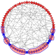
(a) Quantity-imbalance.

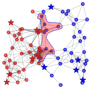
(b) Position-imbalance.

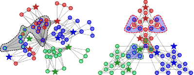
(c) Hierarchy-imbalance.

Figure 1. Representative cases of imbalanced node classification on the graphs by label propagation. Colors represents different types of nodes, where the fill colors of nodes represent the ground truth and the border colors represent the classification result by label propagation. Incorrect results are marked with the dashed regions. The star and circular symbols represent the labeled nodes and unlabeled nodes, respectively.

Due to the cost of labeling in the real-world, the number of labels in different classes is always imbalanced. Most of the existing studies on imbalanced learning of graphs focus on the imbalanced number of labeled nodes in different classes, i.e., quantity-imbalance (Sun et al., 2009; He and Garcia, 2009; Haixiang et al., 2017; Lin et al., 2017; Park et al., 2021; Wang et al., 2021), and a toy example as shown in Figure 1 (a). With the in-depth study of the topological properties and the learning mechanism of GNNs, some recent works have focused on the problem of an unbalanced distribution of labeled nodes in topological positions, i.e., topological position imbalance. The (topological) position-imbalance (Chen et al., 2021; Song et al., 2022; Sun et al., 2022) is caused by the uneven location distribution of labeled nodes in the topological space. As shown in Figure 1 (b), since the graph neural networks (Kipf and Welling, 2017; Velickovic et al., 2018; Hamilton et al., 2017) learn node representations in the message-passing paradigm (Gilmer et al., 2017), even if the labeled nodes have balanced quantity, the uneven position distribution of nodes leads to low-quality of label propagation. However, the existing works (Chen et al., 2021; Song et al., 2022; Sun et al., 2022) only focus on the position and neighborhood information of nodes in the topology structure, and they are difficult to handle the label imbalance issue caused by implicit topological properties of graphs. To sum up, the imbalance issue exploring the topological properties is still in its infancy.

Hierarchy-imbalance issue. Hierarchy is an important topological property of graphs, which simultaneously reproduces the unique properties of scale-free topology and the high clustering of nodes (Ravasz and Barabási, 2003; Vázquez et al., 2002) and can be widely observed in nature, from biology to language to some social networks (Ravasz and Barabási, 2003; Albert et al., 1999), and reflects the important role of nodes in the network. Since graphs with the hierarchical structures are scale-free (with an exponential number growth of nodes and power-law degree distribution) (Barabási and Albert, 1999) and highly modularity (with high connectivity) (Dorogovtsev et al., 2002), it is difficult to measure label imbalance on hierarchical graphs simply by the quantity and location of nodes. For example, the graph in Figure 1 (c) with a hierarchical structure has a balanced quantity (with the same number of labeled nodes in each class) and balanced position (with the same shortest distance to the graph center and degree distribution) of labeled nodes. However, the blue- and green-class labeled nodes occupy higher hierarchy-level roles, resulting in a large number of errors in the classification results. It can be observed that the distribution of labeled nodes in the hierarchy can seriously affect the decision boundary shift of the classifier. Compared with quantity- and position-imbalance issues, exploring the hierarchy-imbalance issue has two major challenges: (1) Implicit topology: hierarchy-imbalance is caused by the uneven distribution of labeled nodes in implicit topological properties, which is difficult to measure intuitively. (2) Hierarchical connectivity: hierarchy of the graph introduces more complex connectivity patterns for nodes, which are difficult to be directly observed and quantified in a single way. Therefore, a natural problem is, ”How to effectively and efficiently measure the hierarchy for each node of graphs, and how does hierarchy-imbalanced label information affect the classification results by the message-passing mechanism? ”

Present work. To solve the above problem, we first give a quantitative analysis for understanding and explore the hierarchy-imbalance issue. Furthermore, inspired by the success of hyperbolic graph learning (Nickel and Kiela, 2017; Tifrea et al., 2019; Chami et al., 2019) for hierarchy-preserving (Krioukov et al., 2010; Papadopoulos et al., 2012), we propose an effective metric to measure the hierarchy of labeled nodes using hyperbolic geometric embedding. Then we propose a novel Hyperbolic Geometric Hierarchy-IMBAlance Learning (HyperIMBA) framework to re-weight the label information propagation and adjust the objective margin accordingly based on the node hierarchy. The key insight of HyperIMBA is to use the graph geometric method to deal with the imbalance issue caused by the topological geometric properties. Specifically, based on the Poincaré model, we design a novel Hierarchy-Aware Margin (HAM) to reduce the decision boundary bias caused by hierarchy-imbalance labeled nodes. Then we design a Hierarchy-aware Message-Passing Neural Network (HMPNN) mechanism based on the class-aware Ricci curvature weight, which measures the influence from the label information and connectivity of neighborhood, alleviating the over-squashing caused by message-passing of cross-hierarchy connectivity pattern by re-weight the ”backbone” paths. Overall, the contributions are summarized as follows:

• For the first time, we explore the hierarchy-imbalance node representation learning as a new issue of topological imbalance topic for semi-supervised node classification.

• We propose a novel training framework, named HyperIMBA, to alleviate the hierarchy-imbalance issue by designing two key mechanisms: HAM captures the implicit hierarchy of labeled nodes to adjust the decision boundary margins, and HMPNN re-weights the path of supervision information passing according to the cross-hierarchy connectivity pattern.

• Extensive experiments on synthetic and real-world datasets demonstrate a significant and consistent improvement and provide insightful analysis for the hierarchy-imbalance issue.

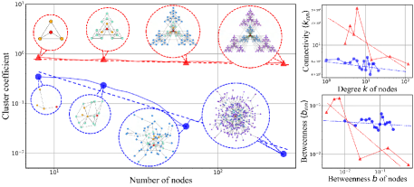
(a) Quantitative analysis of hierarchical network.

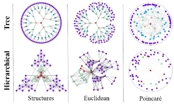
(b) Tree, hierarchical structure in hyperbolic space.

Figure 2. (a) The quantitative analysis of the hierarchical graph and the Barabási–Albert graph. With the growth of the network scale, the cluster coefficients of BA networks are referred to as the power-law distribution, and the cluster coefficients of the hierarchical network vary independently of the scale of the network. The connectivity correlation analysis shows that the nodes tend to connect nodes with similar connectivity and betweenness in BA networks, and the low-degree nodes of the hierarchical network tend to connect to the core nodes. (b) Compared with the Euclidean embedding method, the Poincaré Model can better represent the hierarchy of nodes in hyperbolic space.

2. Preliminary

In this section, we briefly introduce some notations and key definitions. Our work focuses on exploring the relationship between the imbalance issue and hierarchical geometric properties of labeled nodes in the semi-supervised node classification task on graphs.

2.1. Semi-supervised Node Classification

Given a graph $\mathcal{G}=\{\mathcal{V},\mathcal{E}\}$ with the node set $\mathcal{V}$ of $N$ nodes and the edge set $\mathcal{E}$. Let $\mathbf{A}\in\mathbb{R}^{N\times N}$ be the adjacency matrix and $\mathbf{X}\in\mathbb{R}^{N\times d}$ be the node feature matrix, where $d$ denotes the dimension of node features. For node $v$, its neighbors set is $N(v):\{u\in\mathcal{V}|u,v\in\mathcal{E}\}.$ $d_{v}:|\mathcal{N}(v)|$ is the degree of node $v$. Given the labeled node set $\mathcal{V}_{L}$ and their labels $\mathcal{Y}_{L}$ where each node $v_{i}$ is associated with a label $y_{i}$, semi-supervised node classification aims to train a node classifier $f_{\theta}:v\rightarrow\mathbb{R}^{C}$ to predict the labels $\mathcal{Y}_{U}$ of remaining unlabeled nodes $\mathcal{V}_{U}=\mathcal{V}\setminus\mathcal{V}_{L}$, where $C$ denotes the number of classes. We separate the labeled node set $\mathcal{V}_{L}$ into $\{\mathcal{V}^{1}_{L},\mathcal{V}^{2}_{L},\cdots,\mathcal{V}^{C}_{L}\}$, where $\mathcal{V}^{i}_{L}$ denotes the nodes of class $i$ in $\mathcal{V}_{L}$. We focus on semi-supervised node classification based on GNNs methods.

2.2. Hyperbolic Geometric Model

Hyperbolic space is commonly referred to a manifold with constant negative curvature and is used for modeling complex networks. In hyperbolic geometry, five common isometric models are used to describe hyperbolic spaces (Cannon et al., 1997). In this work, we use the Poincaré disk model to reveal the underlying hierarchy of the graph.

Definition 1 (Poincaré disk Model).

The Poincaré Disk Model is a two-dimensional model of hyperbolic geometry with nodes located in the unit disk interior, and the generalization of n-dimensional with standard negative curvature $c$ is the Poincaré ball $\mathcal{B}^{n}_{c}=\{\boldsymbol{x}\in\mathbb{R}^{n}:\left\|\boldsymbol{x}\right\|^{2}<1/c\}$. For any point pair $(\boldsymbol{x},\boldsymbol{y})\in\mathcal{B}^{n}_{c}$, $\boldsymbol{x}\neq\boldsymbol{y}$, the distance on this manifold is defined as:

(1) $$d_{\mathcal{B}^{n}_{c}}(\boldsymbol{x},\boldsymbol{y})=\frac{2}{\sqrt{c}}\tanh^{-1}(\sqrt{c}\left\|-\boldsymbol{x}\oplus_{c}\boldsymbol{y}\right\|),$$

where $\oplus_{c}$ is Möbius addition and $\left\|\cdot\right\|$ is $L_{2}$ norm.

Definition 2 (Poincaré norm).

The Poincaré Norm is defined as the distance of any point $\boldsymbol{x}\in\mathcal{B}^{n}_{c}$ from the origin of Poincaré ball:

(2) $$\left\|\boldsymbol{x}\right\|_{\mathcal{B}^{n}_{c}}=\frac{2}{\sqrt{c}}\tanh^{-1}(\sqrt{c}\left\|\boldsymbol{x}\right\|).$$

3. Understanding Hierarchy-imbalance

In this section, we present a novel hierarchy-imbalance issue for semi-supervised node classification on graphs. Then a quantitative analysis of how the hierarchical nature of the graph affects the representation learning of nodes is presented. Finally, we present a new insight on the hierarchy-imbalance issue of graphs from a hyperbolic geometric perspective.

3.1. Hierarchy-imbalance of Node Classification

The quantity and quality of the information received by a node determine the expressiveness of its representation in GNNs. In graphs with an intrinsic hierarchical structure, hierarchy is highly correlated with both the quantity and quality of information a node can receive. We argue that the imbalance of the node hierarchical tag affects the performance of GNNs in two aspects:

(1) Implicit hierarchy-level: Considering the node label quality, the topological roles of labeled nodes are also highly relevant to the propagation of supervision information. Under the condition that the supervision information decays with the topological distance (Buchnik and Cohen, 2018), the further the quality supervision information can achieve by propagation, the more significant influence the nodes can receive.

(2) Cross-hierarchy connectivity pattern: The hierarchical structure will introduce extra correlations in the graph topology, with the potential to cause nodes at different levels to have different patterns of neighborhood connectivity. The message-passing of supervision and other information may cause an over-squashing problem when the messages are across different hierarchy-levels with narrow connectivity (Topping et al., 2022). The reason is that there are narrow ”bottlenecks” between hierarchy-levels with different connectivity.

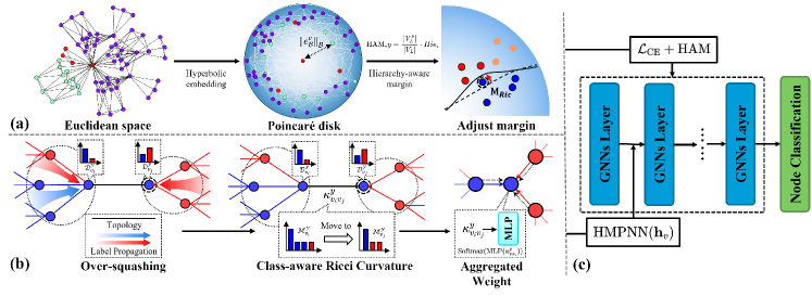
Figure 3. An illustration of HyperIMBA  architecture. (1) HyperIMBA  learns the hyperbolic embedding and the hierarchy of each node by Poincaré model, then gets the hierarchy-aware margin and adds it to the GNNs loss to adjust the decision boundaries; (2) HyperIMBA  calculates class-aware Ricci curvature for each edge, then transforms the Ricci curvatures to aggregated weights by an MLP and Softmax function. (3) HyperIMBA  performs as GNNs with HAM and HMPNN for the node classification.

3.2. Quantitative Analysis of Hierarchical Structure

To further understand the hierarchy-imbalance issue, we use well-known graph models to generate two types of synthetic graphs for quantitative analysis: (a) Hierarchical graph: It is a deterministic fractal and scale-free graph with a 4-nodes module and 4-levels hierarchy and is generated by the Hierarchical Network Model (Ravasz and Barabási, 2003), (b) Barabási–Albert (BA) graph: It is a random scale-free graph with power-law distributions and generated by the extended Barabási–Albert Model (Albert and Barabási, 2000).

Hierarchy and topological properties. Most classification methods based on graph topology rely on the modularity of graphs: the model can easily identify a set of nodes that are closely connected to each other within the class, but with few or no links to nodes outside the class (Albert and Barabási, 2000). These clearly identifiable modular organizations have intuitive decision boundaries on the topology (Figure 1 (b)). As shown in Figure 2 (a) left plot, unlike the BA scale-free graph model in which the clustering coefficients are independent of the degree of a particular node, the clustering coefficients in a hierarchical network can be expressed by a function of degree, i.e., $C(k)=k^{-\beta}$, and the exponent $\beta=1$ in deterministic scale-free networks (Dorogovtsev et al., 2002). It indicates that the decision boundaries may be implicit in the hierarchical topology (Figure 1 (b)). To sum up, the topological role importance of labeled nodes in the hierarchy can more effectively affect the decision boundaries between node classes.

Hierarchy and correlations. The nodes with different hierarchy-levels have different connection patterns on the hierarchical graph. To quantitatively analyze the local topological properties of nodes in the hierarchical network to reveal the connection patterns of different nodes, we consider two important local topological properties, connectivity(degree) and betweenness of nodes, where high connectivity represents nodes that are easier to propagate information, and high betweenness represents nodes that are on the ”backbone” paths of the graph. To quantify the graph propagation patterns across levels of hierarchy, we compute the corresponding average nearest neighbor connectivity $\left\langle k_{nn}\right\rangle$ and betweenness $\left\langle b_{nn}\right\rangle$ of nodes with connectivity $k$ and betweenness $b$ as:

(3) $$\left\langle k_{nn}\right\rangle=\sum_{k^{\prime}}k^{\prime}\operatorname{prob}\left(k^{\prime}\mid k\right),\left\langle b_{nn}\right\rangle=\sum_{b^{\prime}}b^{\prime}\operatorname{prob}\left(b^{\prime}\mid b\right),$$

where $k^{\prime}$ and $b^{\prime}$ are connectivity and betweenness of other nodes, respectively. The results are shown in Figure 2 (a) right plots. For BA graph (blue lines), both $\left\langle k_{nn}\right\rangle$ and $\left\langle b_{nn}\right\rangle$ show that nodes tend to connect with other nodes whose connectivity and betweenness are similar to themselves. For the hierarchical graph (red lines), the $\left\langle k_{nn}\right\rangle$ results indicate that the nodes are more likely to connect to nodes at other different levels, and the $\left\langle b_{nn}\right\rangle$ results reveal that more nodes on ”backbone” paths are more frequently connected with the nodes in the local group. For example, these hierarchical properties on the Internet are likely driven by several additional factors, such as economic market demand. In conclusion, the quantitative analysis shows that the local connectivity and betweenness are closely related to the hierarchy of nodes, and the topological bottleneck of the graph may exist between different hierarchy-levels, which aggravates the over-squashing problem in the message-passing of supervision information.

3.3. Hierarchy of Hyperbolic Geometry Perspective

Hyperbolic space can be understood as smooth versions of trees abstracting the hierarchical organization of complex networks (Krioukov et al., 2010). Figure 2 (b) shows the node embeddings of the tree, hierarchical graphs on Euclidean and hyperbolic space. We can observe that the graph size grows as the radius of the Poincaré disk increases, and the hierarchy deepens as the graph size grows in hyperbolic space. Even though the hierarchical graph has a more complex structure, the position distribution of its hyperbolic embeddings is similar to a tree in hyperbolic space. In the GNNs community, learning the geometric properties of graphs has attracted much attention, and a typical case is learning the hierarchical structure of graphs using hyperbolic geometry (Kennedy et al., 2016; Ganea et al., 2018; Nickel and Kiela, 2017). In summary, hyperbolic geometry provides us with exciting ways to capture and measure the implicit hierarchical structure of graphs.

4. HyperIMBA Model

In this section, we present a novel hyperbolic geometric hierarchy-imbalance learning (HyperIMBA) training framework to address the two main challenges of hierarchy-imbalance. The key insight is that we leverage hyperbolic geometry to abstract the implicit hierarchy of nodes in the graph and introduce a discrete geometric metric to deal with the over-squashing problem of supervision information propagated between hierarchy-levels. The architecture is shown in Figure 3, and the overall process of HyperIMBA is shown in Algorithm 1.

4.1. Hyperbolic Hierarchy-aware Margin

Our goal is to capture the implicit hierarchy of each labeled node, which is an important global property in a hierarchical graph to adjust the decision boundaries in the learning process. To this end, we design the Hyperbolic Hierarchy-Aware Margin (HAM), which consists of three steps: First, we use the topological information of the graph to learn a hyperbolic embedding of the graph by using the Poincaré model. The hierarchical weights of nodes are then learned using their hyperbolic embeddings. Finally, a hyperbolic level-aware margin is designed to modify the objective function.

Step-1: Hyperbolic Embedding of Labeled Nodes. Poincaré embedding (Nickel and Kiela, 2017) is a shallow method of learning embedding into an $n$-dimensional Poincaré ball $\mathcal{B}^{n}_{c}$. In our work, we utilize Poincaré embedding to find the optimal embeddings of nodes by minimizing a hyperbolic distance-based loss function. Based on the hyperbolic distance in Equation 1, the loss function of Poincaré embedding is defined as follows:

(4) $$\mathcal{L}_{\mathcal{B}^{n}_{c}}(\Theta)=\sum_{(u,v)\in\mathcal{E}}\log\frac{e^{-d_{\mathcal{B}^{n}_{c}}(\boldsymbol{u},\boldsymbol{v})}}{\sum_{\boldsymbol{v}^{\prime}\in\mathrm{Neg}(u)}e^{-d_{\mathcal{B}^{n}_{c}}\left(\boldsymbol{u},\boldsymbol{v}^{\prime}\right)}},$$

where the negative examples $\mathrm{Neg}(u)$ of $u$ is $\mathrm{Neg}(u)=\{v|{u,v}\notin\mathcal{E}\}\cup\{u\}$. Then we utilize the stochastic Riemannian optimization method to solve the optimization problem as:

(5) $$\Theta^{\prime}\leftarrow\underset{\Theta}{\arg\min}\mathcal{L}(\Theta)\quad\text{ s.t. }\forall\theta_{i}\in\Theta:\left\|\theta_{i}\right\|<{1/c}.$$

We follow Poincaré embedding using Riemannian stochastic gradient descent (Bonnabel, 2013) to update the model parameters. For each labeled node $v\in\mathcal{V}_{L}$, we get the hyperbolic embedding $e^{v}_{\mathcal{B}}$ by Poincaré embedding method to capture the hierarchy of the node.

Step-2: Hyperbolic Hierarchy-aware Margin. In hyperbolic geometric space, the hyperbolic distance (radius) $R$ of an embedded node from the hyperbolic disk origin (North Pole) is able to abstract the depth of the hidden tree-like hierarchy (Krioukov et al., 2010). In our work, we compute the hyperbolic radius according to Equation 2 as the hierarchy of nodes by computing the Poincaré norm of the hyperbolic node embedding, and then we use a Multi-layer Perceptron (MLP) to transform the Poincaré norm into the hierarchy weights of the nodes. For each node $v\in\mathcal{V}$, the Hierarchy-aware Margin is defined as:

(6) $$\operatorname{HAM}_{v^{y}}=\frac{|\mathcal{V}^{y}_{L}|}{|\mathcal{V}_{L}|}\operatorname{Softmax}\left(\operatorname{MLP}\left(\left\|e^{v}_{\mathcal{B}}\right\|_{\mathcal{B}}\right)\right).$$

Step-3: Objective Function Adjustment. In Section 3.2, we observe the hierarchy of a labeled node represents its global topological role and importance. Inspired by the margin-based imbalance handling methods (Song et al., 2022), we design the Hierarchy-Aware Margin to adaptively handle the intensity of supervision information based on a hierarchy to adjust the decision boundaries. The HyperIMBA learning objective function is formulated as:

(7) $$\mathcal{L}=\frac{1}{\|\mathcal{V}\|}\sum_{v\in\mathcal{V}}\mathcal{L}_{\operatorname{GNNs}}\left(\operatorname{HMPNN}(\boldsymbol{h}_{v})+\alpha\mathrm{HAM},y_{v}\right),$$

4.2. Hierarchy-aware Message-passing

Although HAM can adjust the intensity of the supervision information on global topology, it cannot recognize the hierarchical connectivity patterns of individual nodes. Based on the observations in Section 3.2, we draw a conclusion that a node of hierarchical graph tends to connect nodes with different connectivity (degree) and betweenness, and this cross-hierarchy connectivity pattern is more likely to lead to topology bottlenecks in message-passing.

Class-aware Ricci curvature. Recently, Ricci curvature has been introduced to analyze and measure the over-squashing problem caused by topological bottlenecks (Topping et al., 2022). Inspired by this work, we extend Ollivier-Ricci curvature (Ollivier, 2009) as the edge weights to affect message-passing, which can alleviate the over-squashing problem. Specifically, we first consider the label $i$ distribution in the one-hop neighborhood of a node $u$ is defined as:

(8) $$D_{u,i}=\frac{\left|\left\{v\in\mathcal{N}(u)\mid y=i\right\}\right|}{\|\mathcal{N}(u)\|}.$$

Our class-aware Ricci curvature $\kappa(u,v)_{c}$ of the edge $(u,v)$ is defined as:

(9) $$\kappa(u,v) =\frac{W(m^{y_{u}}_{u},m^{y_{v}}_{v})}{d(u,v)},$$

where $W(\cdot,\cdot)$ is the Wasserstein distance, $d(\cdot,\cdot)$ is the geodesic distance (embedding distance), and $m^{y_{u}}_{u}$ is the mass distribution of node $u$. The mass distribution represents the important distribution of a node and its one-hop neighborhood (Ollivier, 2009), and we further consider the label distribution in the neighborhood as:

$$m^{\alpha,p}_{u}(u_{i},D^{y_{u_{i}}}_{u_{i}})=\begin{cases}\alpha&\mbox{ if }u_{i}=x\\ \frac{1-\alpha}{C}\cdot b^{-D^{y_{u_{i}}}_{u_{i}}d(u,u_{i})^{p}}&\mbox{ if }u_{i}\in\mathcal{N}(u)\\ 0&\mbox{ otherwise }\end{cases},$$

where $C=\sum_{u_{i}\in\mathcal{N}(u)}b^{-d(u,u_{i})^{p}}$. $\alpha$ and $p$ are hyper-parameters that represent the importance of node $x$ and we take $\alpha=0.5$ and $p=2$ following the existing works (Sia et al., 2019; Ye et al., 2019).

Input: Graph $\mathcal{G}=\{\mathcal{V},\mathcal{E}\}$ with node labels $\mathcal{Y}$; Number of training epochs $E$; Loss hyperparameter $\alpha$

1 Parameter $\theta$ initialization;

Output: Predicted label $\hat{\mathcal{Y}}$.

// Learn hierarchy of nodes

2 Learning node Poincaré embedding $e_{\mathcal{B}}\leftarrow$ Equation (4);

3 Calculate node label distribution ${D}\leftarrow$ Equation (8);

4 Calculate class-aware Ricci curvature $\kappa\leftarrow$ Equation (9);

5 for $e=1,2,\cdots,E$ do

       // Learn hyperbolic hierarchy-imbalance margin

6       Calculate the $\operatorname{HAM}\leftarrow$ Equation (6);

       // Hierarchy-aware message-passing

7       Learning curvature-aware $\operatorname{HMPNN}\leftarrow$ Eq. (10);

8       Predict node labels $\hat{\mathcal{Y}}$ $\leftarrow$ Eq. (7);

       // Optimize

9       Calculate the classification loss $\mathcal{L}\leftarrow$ Eq. (7),

10       Update model parameters $\theta$ $\leftarrow\theta-\eta\nabla\theta$.

11 end for

Algorithm 1 HyperIMBA

Curvature-Aware Message-Passing. Class-aware Ricci curvature measures how easily the label information flows through an edge and can be used to guide message-passing. We follow (Ye et al., 2019) by using an MLP to learn the mapping function from the curvature to the aggregated weights $\tau_{uv}$ of MPNN. We have Hierarchy-aware Massage-Passing Neural Networks (HMPNN) as follow:

(10) $$\tau_{uv} =\operatorname{Softmax}\left(\operatorname{MLP}\left(\kappa(u,v)\right)\right),$$

$$\boldsymbol{h}_{i}^{l+1} =U^{l}\left(\boldsymbol{h}_{i}^{l},\sum_{j\in\mathcal{N}(i)}M^{l}\left(\boldsymbol{h}_{i}^{l},\boldsymbol{h}_{j}^{l},\tau_{ij}e_{ij}\right)\right).$$

Table 1. Statistics of real-world datasets.

Dataset		#Node	#Edge	#Label	#Avg. Deg	#$\mathcal{H}$($\mathcal{G}$)
	Cora	2,708	5,429	7	4.01	0.83
	Citeseer	3,327	4,732	6	2.85	0.72
	Photo	7,487	119,043	8	31.80	0.83
	Actor	7,600	33,544	5	8.83	0.24
	Chameleon	2,277	31,421	5	27.60	0.25
	Squirrel	5,201	198,493	5	76.33	0.22

5. Experiment

In this section, we conduct comprehensive experiments to demonstrate the effectiveness and adaptability of HyperIMBA  on various datasets and tasks. We further analyze the robustness to investigate the expressiveness of HyperIMBA.

Table 2. Weighted-F1 score and Micro-F1 score (% ± standard deviation) of node classification on real-world graph datasets.
(Result: average score ± standard deviation; Bold: best; Underline: runner-up; The hyphen symbol indicates experiments results are not accessible due to memory issue or time limits.)

	Model	Cora		Citeseer		Photo		Actor		Chameleon		Squirrel
		W-F1	M-F1	W-F1	M-F1	W-F1	M-F1	W-F1	M-F1	W-F1	M-F1	W-F1	M-F1
GCN	original	79.4±0.9	77.5±1.5	66.3±1.3	62.2±1.2	85.4±2.8	84.6±1.3	21.8±1.3	20.9±1.4	30.5±3.4	30.5±3.3	21.9±1.2	21.9±1.2
	ReNode	80.0±0.7	78.4±1.3	66.4±1.0	62.4±1.1	86.2±2.4	85.3±1.6	21.2±1.2	20.2±1.6	30.3±3.2	30.4±2.8	22.4±1.1	22.4±1.1
	DropEdge	79.8±0.8	77.8±1.0	66.6±1.4	63.4±1.6	86.8±1.7	85.4±1.3	22.4±1.0	21.4±1.3	30.6±3.5	30.6±3.3	22.8±1.2	22.8±1.2
	SDRF	82.1±0.8	79.3±1.0	69.6±0.4	66.6±0.3	-	-	-	-	32.3±0.7	39.0±1.2	-	-
	ReNode+TAM	80.1±0.9	78.2±1.6	67.1±1.4	62.3±0.9	87.6±1.3	86.9±1.0	23.1±0.9	22.2±1.3	32.3±0.9	32.1±0.8	22.1±0.4	22.1±0.3
	HyperIMBA	83.0±0.3	83.1±0.4	76.3±0.2	73.4±0.3	92.8±0.3	92.5±0.3	30.7±0.2	29.3±0.4	44.1±0.7	42.3±1.1	31.2±2.4	28.4±2.0
GAT	original	78.3±1.5	76.4±1.7	64.4±1.7	60.6±1.7	88.2±2.9	86.2±2.6	21.8±1.2	20.9±1.1	29.9±3.5	29.9±3.1	20.5±1.4	20.5±1.4
	ReNode	78.9±1.2	77.2±1.5	64.9±1.6	61.0±1.5	89.1±2.4	87.1±2.6	21.5±1.2	20.5±1.1	29.2±2.3	29.1±2.0	20.4±1.8	20.4±1.8
	DropEdge	78.7±1.3	76.9±1.5	64.5±1.4	60.5±1.3	88.9±1.9	87.1±2.1	22.9±1.2	21.8±1.1	30.3±1.6	30.2±1.2	21.2±1.5	21.2±1.5
	SDRF	77.9±0.7	75.9±0.9	64.9±0.6	61.9±0.9	-	-	-	-	43.0±1.9	42.5±1.9	-	-
	ReNode+TAM	78.4±1.3	77.3±1.3	64.2±1.3	63.1±0.8	89.0±1.8	87.3±1.7	21.3±1.2	20.7±1.1	30.9±1.5	30.2±1.8	20.0±1.4	19.4 ±1.2
	HyperIMBA	83.5±0.3	83.6±0.3	75.0±0.4	73.0±0.4	92.5±0.5	92.1±0.8	30.9±1.0	29.8±1.0	43.2±0.7	42.5±0.6	31.1±1.0	28.7±1.3
GraphSAGE	original	75.4±1.6	74.1±1.6	64.8±1.6	60.7±1.6	86.1±2.5	83.3±2.4	24.0±1.2	23.2±1.0	36.5±1.6	36.2±1.6	27.2±1.7	27.2±1.7
	ReNode	76.4±0.9	75.0±1.1	65.4±1.7	61.2±1.7	86.5±1.7	84.1±1.7	23.7±1.2	22.8±1.0	36.4±1.9	36.1±1.9	27.7±1.8	27.7±1.8
	DropEdge	76.0±1.6	74.5±1.6	65.1±1.4	60.9±1.4	86.2±1.6	83.5±1.4	24.1±1.0	23.3±0.9	37.5±1.4	37.2±1.4	27.5±1.8	27.5±1.8
	SDRF	75.7±0.8	74.6±0.8	65.3±0.6	61.4±0.6	-	-	-	-	41.5±2.6	41.6±2.7	-	-
	ReNode+TAM	76.0±1.1	74.9±1.0	67.1±2.0	63.4±1.2	86.4±1.4	83.8±1.2	23.6±1.2	22.5±1.3	38.3±1.8	38.1±1.8	27.8±1.4	27.8±1.4
	HyperIMBA	72.4±0.3	71.5±0.5	72.8±0.2	70.5±0.3	80.9±1.2	78.2±1.2	35.6±0.6	34.3±1.1	42.9±0.6	42.5±0.6	38.6±1.1	36.9±0.7

Table 3. Weighted-F1 scores (% ± standard deviation) and improvements (%) results of Ablation Study. (Result: average score ± standard deviation; Bold: best.)

Model	Cora		Citeseer		Photo		Actor		Chameleon		Squirrel
	W-F1 (%)	$\Delta$ (%)	W-F1 (%)	$\Delta$ (%)	W-F1 (%)	$\Delta$ (%)	W-F1 (%)	$\Delta$ (%)	W-F1 (%)	$\Delta$ (%)	W-F1 (%)	$\Delta$ (%)
GCN	79.4±0.9	-	66.3±1.3	-	85.4±2.8	-	21.8±1.3	-	30.5±3.4	-	21.9±1.2	-
HyperIMBA (w/o HMPNN)	82.3±0.3	$\uparrow$2.9	71.3±0.7	$\uparrow$5.0	92.4±0.3	$\uparrow$7.0	29.6±2.9	$\uparrow$7.8	39.6±0.9	$\uparrow$9.1	24.9±0.8	$\uparrow$3.0
HyperIMBA (w/o HAM)	82.9±0.5	$\uparrow$3.5	75.8±0.5	$\uparrow$9.5	92.6±0.4	$\uparrow$7.2	30.1±0.5	$\uparrow$8.3	42.4±0.9	$\uparrow$11.9	26.3±0.8	$\uparrow$4.4
HyperIMBA	83.0±0.3	$\uparrow$3.6	76.3±0.2	$\uparrow$10.0	92.8±0.3	$\uparrow$7.4	30.7±0.2	$\uparrow$8.9	44.1±0.7	$\uparrow$13.6	31.2±2.4	$\uparrow$9.3

5.1. Datasets

We conduct experiments on synthetic and real-world datasets to evaluate our method, and analyze the model’s capabilities in terms of both graph theory and real-world scenarios. The statistics of the datasets are summarized in Table 1. The edge homophily $\mathcal{H}(\mathcal{G})$ is computed according to (Pei et al., 2020a).

Synthetic Datasets. We generate the hierarchical synthetic graphs for essential verification and analysis of our method by the well-accepted graph theoretical model: Hierarchical Network Model (HNM) (Ravasz and Barabási, 2003). For each dataset, we create 1,024 nodes and subsequently perform the graph generation algorithm on these nodes. For the hierarchical graph, we consider an initial network of $N=4$ fully interconnected nodes as the fractal, and derive $k=5$ times in an iterative way by replicating the initial fractal of the graph according to the fractal structure. For each generated graph, we randomly select 80% nodes as the test set, 10% nodes as the training set, and the other 10% nodes as the validation set.

Real-world Datasets. We also conducted experiments on several real-world datasets: (1) Citation network: Cora and Citeseer (Sen et al., 2008) are citation networks of academic papers. (2) Co-occurrence network: Photo (Shchur et al., 2018) is segment of the Amazon co-purchase graph and Actor (Pei et al., 2020b) is an actor co-occurrence network. (3) Page-page network: Chameleon and Squirrel (Rozemberczki et al., 2021) are page-page networks on Wikipedia. Since we focus on the imbalance issue of topological properties, we set the same number of labeled nodes for each class.

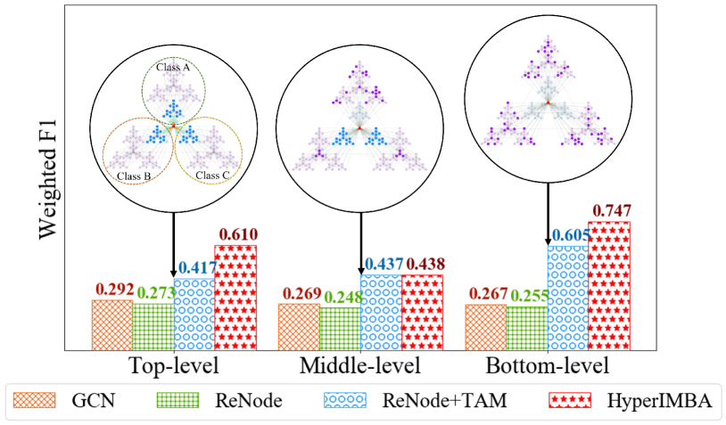
Figure 4. Performances of different hierarchy-level training setup on the synthetic graph.

5.2. Experimental Setup

Baselines. We choose well-known GNNs as backbones, including GCN (Kipf and Welling, 2017), GAT (Velickovic et al., 2018), and GraphSAGE (Hamilton et al., 2017). To evaluate the proposed HyperIMBA, we compare it with a variety of baselines, including: the most relevant baselines of the topology-imbalance issue are ReNode (Chen et al., 2021) and TAM (Song et al., 2022). ReNode is a position-aware and re-weighted (Cao et al., 2019; Cui et al., 2019; Ren et al., 2018) method, and TAM is a neighborhood class information-aware margin-based method. DropEdge (Rong et al., 2019) randomly removes a certain number of edges from the input graph at each training epoch, which acts as data augmentation (Park et al., 2021) in terms of structure. SDRF (Topping et al., 2022) is a structure rewiring method for the over-squashing issue, which modifies edges with Ricci curvatures.

Settings. We set the depth of GNN backbones as 2 layers and adopt the implementations from the PyTorch Geometric Library in all experiments. We set the representation dimension of all baselines and HyperIMBA to 256. The parameters of baselines are set as the suggested value in their papers or carefully tuned. For DropEdge, we set the edge dropping/adding probability to 10%. For HyperIMBA, we set the hyperbolic curvature $c=1$ of Poincaé model.

5.3. Performance Evaluation

Performance on Synthetic Graphs. To verify the hierarchy capturing ability, we evaluate our method on hierarchical organization synthetic graph HNM. The node classes of HNM are three communities with the same hierarchical structure and are evenly distributed in three directions of the graph, as shown in Figure 4. We divide the hierarchical graph into three levels according to the hierarchy-level: the top-level (1, 2, 3-order fractals of HNM), the middle-level (4-order fractals of HNM), and the bottom-level (5-order fractals of HNM), respectively, to verify the effect of the model using labeled nodes at different hierarchy-levels as training samples. We allow randomly sample labeled nodes in low-level to supplement the high-level labeled nodes together as training nodes to reach a consensus for each class. According to Figure 4, HyperIMBA  significantly outperforms all baselines, especially with top-level or bottom-level training setup. In addition, unlike the performance of ReNode and TAM increases monotonically from the top- to bottom-level, the performance of HyperIMBA and vanilla GCN is higher in the top- and bottom-level than in the middle-level. This phenomenon matches perfectly with the hierarchical connectivity pattern which we discussed in Section  3.2, i.e., nodes of a hierarchical graph tend to connect with nodes of different connectivity and betweenness rather than the nodes with similar properties. HyperIMBA benefits from the discrete curvature-aware re-weighting, which effectively alleviates the over-squashing problem caused by cross-hierarchy connectivity pattern.

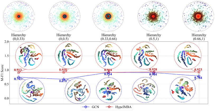
Figure 5. Performances and analyis on Photo with different hierarchy-levels training setting.

Performance on Real-world Graphs. Table 2 summarizes the performance of HyperIMBA  and all baselines on six real-world datasets. Our HyperIMBA shows significant superiority in improving the performance of GCN and GAT on all datasets. It demonstrates that HyperIMBA  is capable of capturing the underlying topology and important connectivity patterns, especially for the backbones that can thoroughly learn the topology. Our method has only a few improvements for the backbone on high homophily and weak hierarchical graphs such as Cora. By contrast, our method achieves an overwhelming advantage on graphs with high heterophily datasets (Actor, Chameleon, and Squirrel). TAM improves the performance of ReNode by considering the label connectivity of the neighborhood, but it still does not work well on the graph with poor connectivity (Citeseer). The reason for the poor performance of ReNode is that topological boundaries are difficult to be directly used as decision boundaries on real-world graphs. Compared with SDRF, HyperIMBA  further considers the over-squashing problem of supervision information, and the improvement of results also confirms our intuition. Note that the performance of HyperIMBA  depends on whether global and higher-order topological properties play an important role in learning. For the subgraph-sampling method (GraphSAGE), HyperIMBA  can still obtain significant improvement in most cases of incomplete topology information.

5.4. Analysis of HyperIMBA

In this subsection, we conduct ablation studies for HAM and HMPNN, to provide further performance analysis for our model. Then we perform a case study of hierarchy-imbalance learning, and provide the observation of the learning performances under different hierarchy-level training settings to explore the intrinsic mechanism of the hierarchy-imbalance issue. We also visualize the learning results to provide further insights into the impact caused by the hierarchy-imbalance issue more intuitively.

Ablation Study. We conduct ablation studies for the two main mechanisms of HyperIMBA, hierarchy-aware margin and hierarchy-aware message-passing. We choose GCN as the backbone, and the results are shown in Table 3. HAM plays a key role in alleviating the hierarchy-imbalance issue, and demonstrate the superiority of hyperbolic geometry for capturing the underlying hierarchy of graphs. Moreover, HMPNN also significantly alleviates the over-compression problem of label supervision information. In summary, HyperIMBA consistently outperforms the GCN and the other two variants on all real-world datasets.

Case study and Visualization. We construct a case study based on the real-world dataset Photo to explore how the labeled nodes at different hierarchy-levels will affect the learning models. We divide five regions in the embedded Poincaré disk of Photo, and randomly sample labeled nodes in the regions as training samples, respectively. In order to satisfy the quantity-balanced setting of labeled nodes for each node class, we also perform a random supplement selection of nodes according to a certain probability as in Subsection 5.3. Figure 5 shows the training setting of five hierarchy-levels and reports the performances and visualizations of GCN and HyperIMBA for each hierarchy-level using t-SNE(Van der Maaten and Hinton, 2008).

As we can observe in Figure 5, the labeled nodes with different hierarchy-levels significantly affect the shapes and boundaries of the node embedding clusters, which indicates that the hierarchical properties can directly affect the decision boundary of the model by handling the connectivity pattern on the graph. An interesting observation is that the top-level labeled nodes make the embedding distribution much more compact and produce a large number of false positives, which indicates that it has a severe over-squashing problem in the message-passing process. It is consistent with the quantitative analysis in Section 3.2, i.e., the nodes with high connectivity and betweenness refer to connect nodes with low connectivity and betweenness according to hierarchical connectivity patterns. In addition, we observe that the bottom-level nodes with more diverse information, resulting in node clusters with diffuse shapes and wider boundaries, may easily lead to conflicts or overlaps between different node classes. The visualization of the results in Figure 5 shows that HyperIMBA consistently maintains the appropriate node cluster shapes and boundaries under different hierarchy-level training settings.

6. Conclusion

In this paper, for the first time, we explore the hierarchy-imbalance issue on the hierarchical structure, which is a significant topological property of the graph. We proposed HyperIMBA, a novel training framework to alleviate the hierarchy-imbalance issue from the hyperbolic geometric perspective. HyperIMBA can effectively capture the implicit hierarchy of nodes by hyperbolic geometric embedding, and we propose a hierarchy-aware margin for adjusting classification decision boundaries. Moreover, HyperIMBA leverages discrete local curvature to improve the message-passing mechanism for alleviating the over-squashing problem caused by hierarchy connectivity patterns. Experimental results on synthetic and real-world datasets demonstrate that HyperIMBA consistently and significantly outperforms existing works.

- (1)
- Albert and Barabási (2000) Réka Albert and Albert-László Barabási. 2000. Topology of evolving networks: local events and universality. Physical review letters 85, 24 (2000), 5234.
- Albert et al. (1999) Réka Albert, Hawoong Jeong, and Albert-László Barabási. 1999. Diameter of the world-wide web. nature 401, 6749 (1999), 130–131.
- Barabási and Albert (1999) Albert-László Barabási and Réka Albert. 1999. Emergence of scaling in random networks. Science 286, 5439 (1999), 509–512.
- Bonnabel (2013) Silvere Bonnabel. 2013. Stochastic gradient descent on Riemannian manifolds. IEEE Trans. Automat. Control 58, 9 (2013), 2217–2229.
- Buchnik and Cohen (2018) Eliav Buchnik and Edith Cohen. 2018. Bootstrapped graph diffusions: Exposing the power of nonlinearity. In SIGMETRICS. 8–10.
- Cannon et al. (1997) James W Cannon, William J Floyd, Richard Kenyon, Walter R Parry, et al. 1997. Hyperbolic geometry. Flavors of geometry 31 (1997), 59–115.
- Cao et al. (2019) Kaidi Cao, Colin Wei, Adrien Gaidon, Nikos Arechiga, and Tengyu Ma. 2019. Learning imbalanced datasets with label-distribution-aware margin loss. In NeurIPS, Vol. 32.
- Chami et al. (2019) Ines Chami, Zhitao Ying, Christopher Ré, and Jure Leskovec. 2019. Hyperbolic Graph Convolutional Neural Networks. In NeurIPS. 4869–4880.
- Chen et al. (2021) Deli Chen, Yankai Lin, Guangxiang Zhao, Xuancheng Ren, Peng Li, Jie Zhou, and Xu Sun. 2021. Topology-Imbalance Learning for Semi-Supervised Node Classification. NeurIPS 34 (2021).
- Cui et al. (2019) Yin Cui, Menglin Jia, Tsung-Yi Lin, Yang Song, and Serge Belongie. 2019. Class-balanced loss based on effective number of samples. In CVPR. 9268–9277.
- Dorogovtsev et al. (2002) Sergey N Dorogovtsev, Alexander V Goltsev, and José Ferreira F Mendes. 2002. Pseudofractal scale-free web. Physical review E 65, 6 (2002), 066122.
- Fu et al. (2021) Xingcheng Fu, Jianxin Li, Jia Wu, Qingyun Sun, Cheng Ji, Senzhang Wang, Jiajun Tan, Hao Peng, and S Yu Philip. 2021. ACE-HGNN: Adaptive Curvature Exploration Hyperbolic Graph Neural Network. In ICDM. IEEE, 111–120.
- Ganea et al. (2018) Octavian-Eugen Ganea, Gary Bécigneul, and Thomas Hofmann. 2018. Hyperbolic Neural Networks. In NeurIPS. 5350–5360.
- Gilmer et al. (2017) Justin Gilmer, Samuel S Schoenholz, Patrick F Riley, Oriol Vinyals, and George E Dahl. 2017. Neural message passing for quantum chemistry. In ICML. 1263–1272.
- Haixiang et al. (2017) Guo Haixiang, Li Yijing, Jennifer Shang, Gu Mingyun, Huang Yuanyue, and Gong Bing. 2017. Learning from class-imbalanced data: Review of methods and applications. Expert systems with applications 73 (2017), 220–239.
- Hamilton et al. (2017) Will Hamilton, Zhitao Ying, and Jure Leskovec. 2017. Inductive representation learning on large graphs. In NeurIPS. 1024–1034.
- He and Garcia (2009) Haibo He and Edwardo A Garcia. 2009. Learning from imbalanced data. IEEE Transactions on knowledge and data engineering 21, 9 (2009), 1263–1284.
- Kennedy et al. (2016) W Sean Kennedy, Iraj Saniee, and Onuttom Narayan. 2016. On the hyperbolicity of large-scale networks and its estimation. In Big Data. IEEE, 3344–3351.
- Kipf and Welling (2017) Thomas N. Kipf and Max Welling. 2017. Semi-Supervised Classification with Graph Convolutional Networks. In ICLR.
- Krioukov et al. (2010) Dmitri Krioukov, Fragkiskos Papadopoulos, Maksim Kitsak, Amin Vahdat, and Marián Boguná. 2010. Hyperbolic geometry of complex networks. Physical Review E 82, 3 (2010), 036106.
- Li et al. (2022) Jianxin Li, Xingcheng Fu, Qingyun Sun, Cheng Ji, Jiajun Tan, Jia Wu, and Hao Peng. 2022. Curvature Graph Generative Adversarial Networks. In WWW. 1528–1537.
- Li et al. (2023) Jianxin Li, Qingyun Sun, Hao Peng, Beining Yang, Jia Wu, and S Yu Phillp. 2023. Adaptive Subgraph Neural Network with Reinforced Critical Structure Mining. IEEE Transactions on Pattern Analysis and Machine Intelligence (2023).
- Lin et al. (2017) Tsung-Yi Lin, Priya Goyal, Ross Girshick, Kaiming He, and Piotr Dollár. 2017. Focal loss for dense object detection. In ECCV. 2980–2988.
- Nastase et al. (2015) Vivi Nastase, Rada Mihalcea, and Dragomir R Radev. 2015. A survey of graphs in natural language processing. Natural Language Engineering 21, 5 (2015), 665–698.
- Nickel and Kiela (2017) Maximilian Nickel and Douwe Kiela. 2017. Poincaré Embeddings for Learning Hierarchical Representations. In NeurIPS. 6338–6347.
- Ollivier (2009) Yann Ollivier. 2009. Ricci curvature of Markov chains on metric spaces. Journal of Functional Analysis 256, 3 (2009), 810–864.
- Papadopoulos et al. (2012) Fragkiskos Papadopoulos, Maksim Kitsak, M Ángeles Serrano, Marián Boguná, and Dmitri Krioukov. 2012. Popularity versus similarity in growing networks. Nature (2012), 537–540.
- Park et al. (2021) Joonhyung Park, Jaeyun Song, and Eunho Yang. 2021. GraphENS: Neighbor-Aware Ego Network Synthesis for Class-Imbalanced Node Classification. In ICLR.
- Pei et al. (2020a) Hongbin Pei, Bingzhe Wei, Kevin Chen-Chuan Chang, Yu Lei, and Bo Yang. 2020a. Geom-GCN: Geometric Graph Convolutional Networks. In ICLR. OpenReview.net.
- Pei et al. (2020b) Hongbin Pei, Bingzhe Wei, Kevin Chen-Chuan Chang, Yu Lei, and Bo Yang. 2020b. Geom-gcn: Geometric graph convolutional networks. In ICLR.
- Ravasz and Barabási (2003) Erzsébet Ravasz and Albert-László Barabási. 2003. Hierarchical organization in complex networks. Physical review E 67, 2 (2003), 026112.
- Ren et al. (2018) Mengye Ren, Wenyuan Zeng, Bin Yang, and Raquel Urtasun. 2018. Learning to reweight examples for robust deep learning. In ICML. PMLR, 4334–4343.
- Rong et al. (2019) Yu Rong, Wenbing Huang, Tingyang Xu, and Junzhou Huang. 2019. Dropedge: Towards deep graph convolutional networks on node classification. In ICLR.
- Rozemberczki et al. (2021) Benedek Rozemberczki, Carl Allen, and Rik Sarkar. 2021. Multi-scale attributed node embedding. Journal of Complex Networks 9, 2 (2021), cnab014.
- Sen et al. (2008) Prithviraj Sen, Galileo Namata, Mustafa Bilgic, Lise Getoor, Brian Galligher, and Tina Eliassi-Rad. 2008. Collective classification in network data. AI magazine 29, 3 (2008), 93–93.
- Shchur et al. (2018) Oleksandr Shchur, Maximilian Mumme, Aleksandar Bojchevski, and Stephan Günnemann. 2018. Pitfalls of graph neural network evaluation. arXiv preprint arXiv:1811.05868 (2018).
- Sia et al. (2019) Jayson Sia, Edmond Jonckheere, and Paul Bogdan. 2019. Ollivier-ricci curvature-based method to community detection in complex networks. Scientific reports 9, 1 (2019), 1–12.
- Song et al. (2022) Jaeyun Song, Joonhyung Park, and Eunho Yang. 2022. TAM: Topology-Aware Margin Loss for Class-Imbalanced Node Classification. In ICML. PMLR, 20369–20383.
- Sun et al. (2021) Qingyun Sun, Jianxin Li, Hao Peng, Jia Wu, Yuanxing Ning, Philip S Yu, and Lifang He. 2021. Sugar: Subgraph neural network with reinforcement pooling and self-supervised mutual information mechanism. In Proceedings of the Web Conference 2021. 2081–2091.
- Sun et al. (2023) Qingyun Sun, Jianxin Li, Beining Yang, Xingcheng Fu, Hao Peng, and Philip S Yu. 2023. Self-organization Preserved Graph Structure Learning with Principle of Relevant Information. In AAAI.
- Sun et al. (2022) Qingyun Sun, Jianxin Li, Haonan Yuan, Xingcheng Fu, Hao Peng, Cheng Ji, Qian Li, and Philip S Yu. 2022. Position-aware Structure Learning for Graph Topology-imbalance by Relieving Under-reaching and Over-squashing. In CIKM. Association for Computing Machinery, 1848–1857.
- Sun et al. (2009) Yanmin Sun, Andrew KC Wong, and Mohamed S Kamel. 2009. Classification of imbalanced data: A review. International journal of pattern recognition and artificial intelligence 23, 04 (2009), 687–719.
- Tifrea et al. (2019) Alexandru Tifrea, Gary Bécigneul, and Octavian-Eugen Ganea. 2019. Poincare Glove: Hyperbolic Word Embeddings. In ICLR.
- Topping et al. (2022) Jake Topping, Francesco Di Giovanni, Benjamin Paul Chamberlain, Xiaowen Dong, and Michael M Bronstein. 2022. Understanding over-squashing and bottlenecks on graphs via curvature. In ICLR.
- Van der Maaten and Hinton (2008) Laurens Van der Maaten and Geoffrey Hinton. 2008. Visualizing data using t-SNE. Journal of machine learning research 9, 11 (2008).
- Vázquez et al. (2002) Alexei Vázquez, Romualdo Pastor-Satorras, and Alessandro Vespignani. 2002. Large-scale topological and dynamical properties of the Internet. Physical Review E 65, 6 (2002), 066130.
- Velickovic et al. (2018) Petar Velickovic, Guillem Cucurull, Arantxa Casanova, Adriana Romero, Pietro Liò, and Yoshua Bengio. 2018. Graph Attention Networks. In ICLR.
- Wang et al. (2021) Yu Wang, Charu Aggarwal, and Tyler Derr. 2021. Distance-wise Prototypical Graph Neural Network in Node Imbalance Classification. arXiv preprint arXiv:2110.12035 (2021).
- Ye et al. (2019) Ze Ye, Kin Sum Liu, Tengfei Ma, Jie Gao, and Chao Chen. 2019. Curvature graph network. In ICLR.
- Yu et al. (2022) Jinze Yu, Jiaming Liu, Xiaobao Wei, Haoyi Zhou, Yohei Nakata, Denis Gudovskiy, Tomoyuki Okuno, Jianxin Li, Kurt Keutzer, and Shanghang Zhang. 2022. Cross-Domain Object Detection with Mean-Teacher Transformer. In ECCV.
- Zhang et al. (2020) Ziwei Zhang, Peng Cui, and Wenwu Zhu. 2020. Deep learning on graphs: A survey. IEEE Transactions on Knowledge and Data Engineering (2020).