Multi-Graph Convolution Network for Pose Forecasting

Abstract

Recently, there has been a growing interest in predicting human motion, which involves forecasting future body poses based on observed pose sequences. This task is complex due to modeling spatial and temporal relationships. The most commonly used models for this task are autoregressive models, such as recurrent neural networks (RNNs) or variants, and Transformer Networks. However, RNNs have several drawbacks, such as vanishing or exploding gradients. Other researchers have attempted to solve the communication problem in the spatial dimension by integrating Graph Convolutional Networks (GCN) and Long Short-Term Memory (LSTM) models. These works deal with temporal and spatial information separately, which limits the effectiveness. To fix this problem, we propose a novel approach called the multi-graph convolution network (MGCN) for 3D human pose forecasting. This model simultaneously captures spatial and temporal information by introducing an augmented graph for pose sequences. Multiple frames give multiple parts, joined together in a single graph instance. Furthermore, we also explore the influence of natural structure and sequence-aware attention to our model. In our experimental evaluation of the large-scale benchmark datasets, Human3.6M[11], AMSS[17] and 3DPW[31], MGCN outperforms the state-of-the-art in pose prediction (See Table 1 and Figure 1).

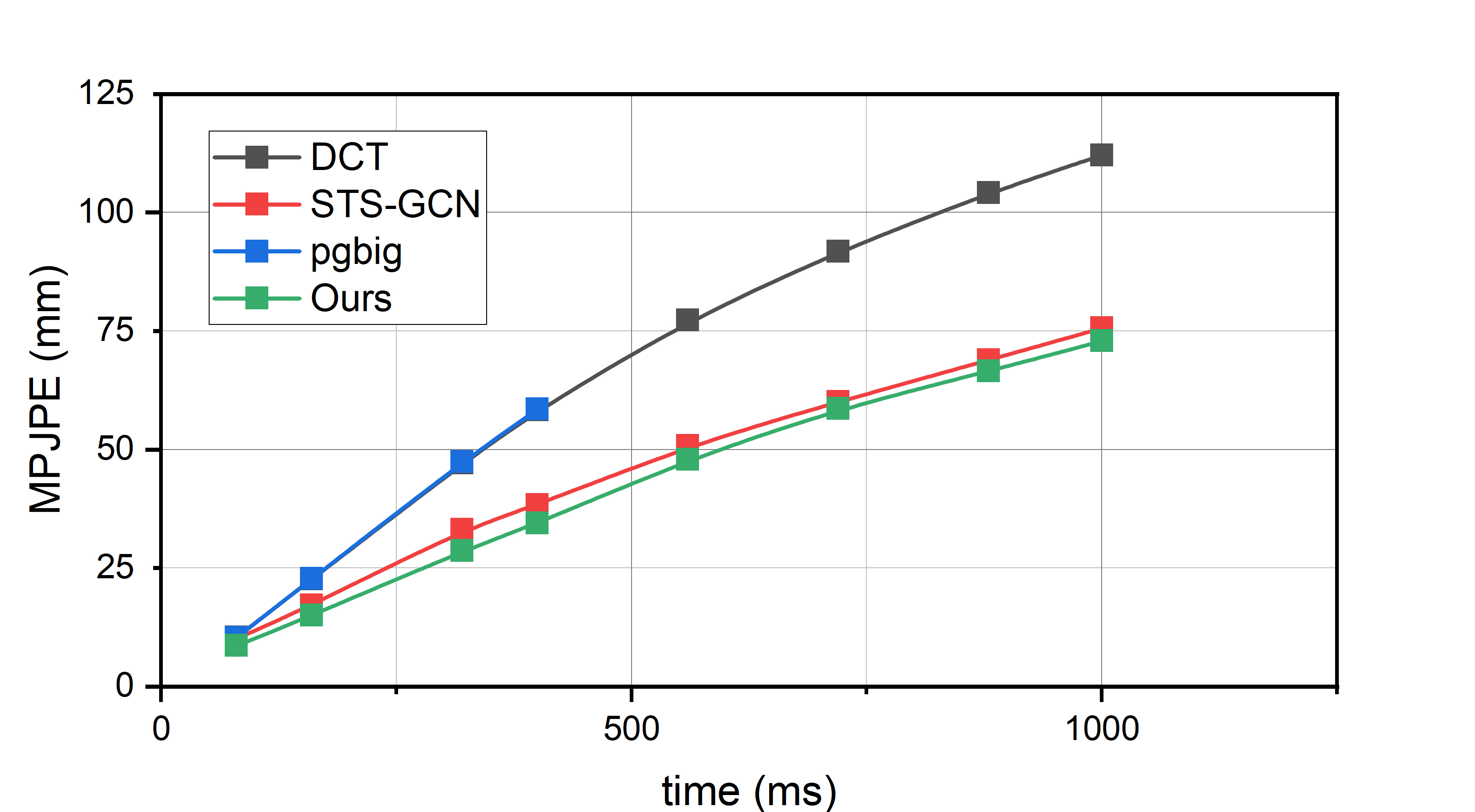
(a)

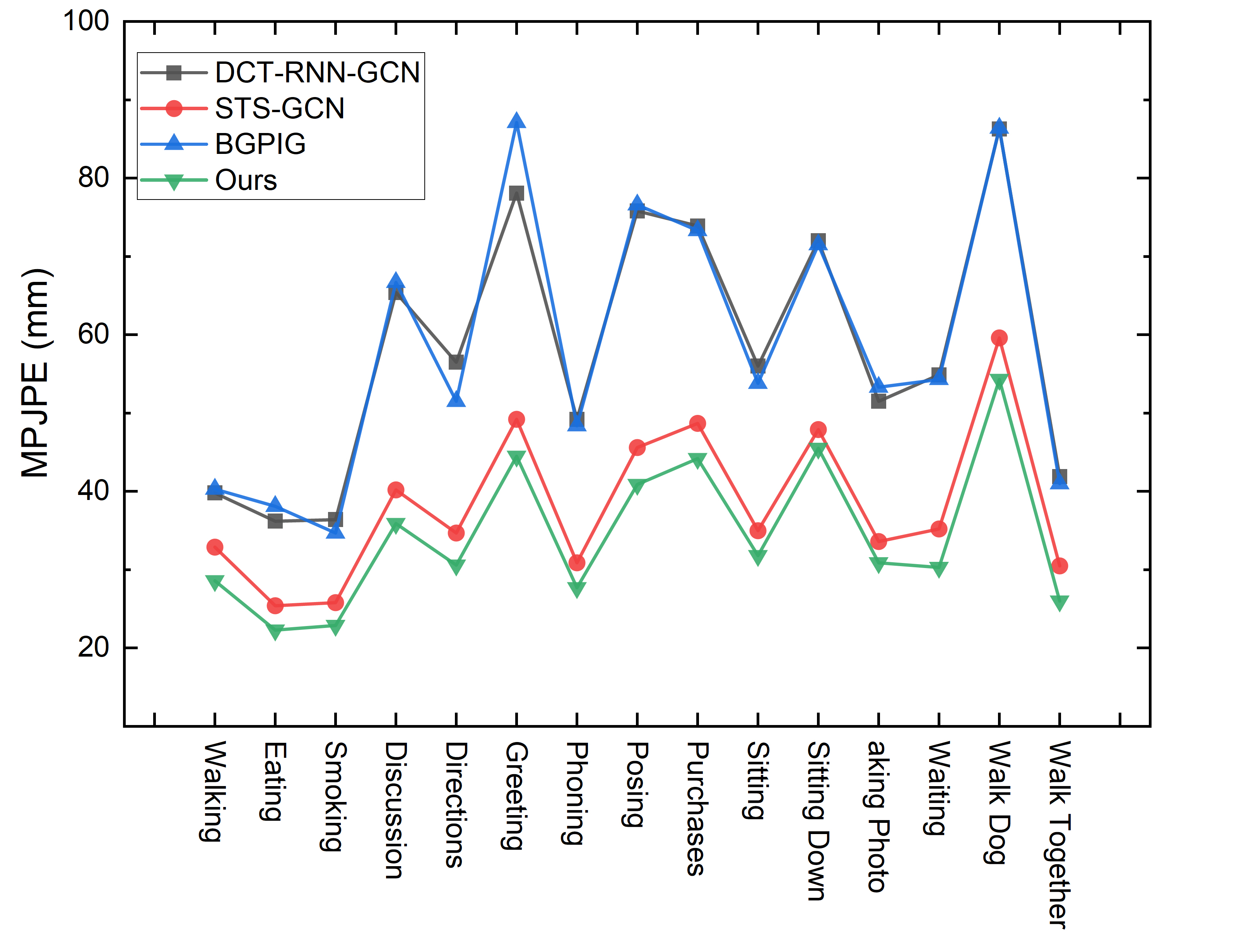
(b)

Figure 1: (a) Performance of various methods on Human3.6M. The figure shows that our method outperforms others and achieves state-of-the-art. (b) Performance of different actions on a 400 ms prediction task.

1 Introduction

Human pose forecasting is a critical task that involves modeling the complete structured sequence of joints. It has various applications in human-robot interaction systems [12], autonomous driving [21], and healthcare [29]. Many researchers [5, 18, 19] use recurrent neural networks (RNNs) or variants to tackle this task due to the sequential nature of the data. However, RNNs have several drawbacks. Firstly, they are prone to vanishing or exploding gradients [22]. Secondly, RNN-based methods often suffer from severe discontinuities between adjacent output frames, leading to poor global smoothing of the output sequence [13, 20]. To tackle these challenges, Graph Convolutional Networks (GCN) have been introduced. GCNs extract features from key point graphs and have achieved state-of-the-art performance on several benchmark datasets, as reported in [24].

Song et al. [25] utilize the connection between different frames for traffic management. Inspired by this, we propose an approach to pose forecasting which simultaneously models spatial and temporal body joints. Specifically, Graph Convolutional networks are employed: a given time instant gives a pose, which is part of the graph. Multiple frames give multiple parts, joined together in a single graph instance. In addition, we have taken inspiration from the autoregressive mechanism and decoder of the Transformer [30] to create a masked attention mechanism. This mechanism allows our model to accurately represent the human pose in frame $t$ using only the feature information prior to frame $t$.

Figure 2 and Figure 3 illustrate the pipeline of our proposed model and the network architecture of MGCN respectively. Firstly, we generate vectors Q, K, and V using MGCN. We adopt a modified attention mechanism and add a mask to the S to perceive the sequences, which we refer to as "sequence-aware attention". Next, we use temporal convolutional networks (TCNs [10, 2]) as a time sequence generator to align the number of frames to predict. Finally, we add a refinement process after the generator to achieve a smoother representation of the output frames.

The main contributions of this paper are summarized as follows:

$\bullet$ A novel multi-graph convolutional network with spatial-temporal reception is proposed.

$\bullet$ We propose two strategies on attention to make the model aware of the sequence, which achieve state-of-the-art at different tasks.

$\bullet$ We experimentally prove the importance of natural links for GCN.

$\bullet$ The proposed model of MGCN significantly exceeds the state-of-the-art in Human3.6M, 3DPW and AMASS benchmarks.

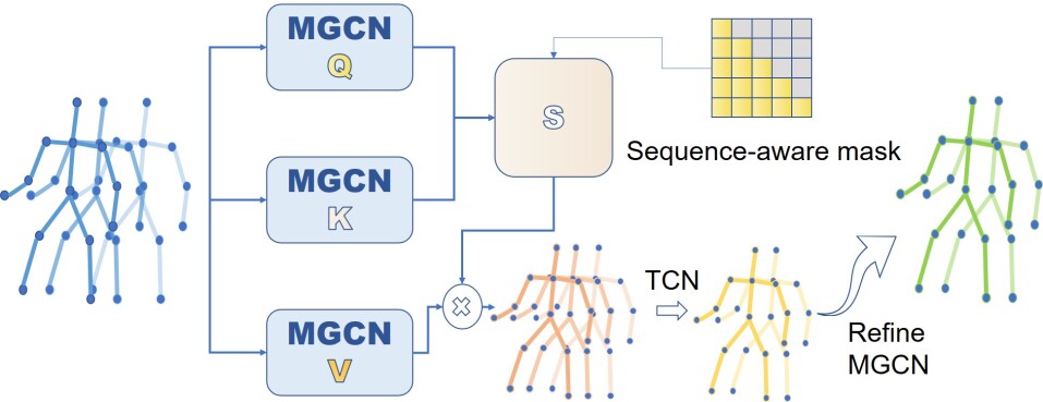
Figure 2: The complete pipelines of the proposed model. The vectors Q, K, and V are all produced by the MGCN. After the masked attention, TCN is applied as a time sequence generator, aligning the number of frames the model will predict. Finally, we use another MGCN module to refine the results.

2 Related Work

Considering whether graph convolution networks are used or not, we divide the recent works related to human pose forecasting into two parts.

No-GCN methods RNN [5, 18, 19] or variants such as gated recurrent units (GRU) [34] or long short-term memory networks (LSTM) [33] have been widely adopted in human pose forecasting. These flexible techniques have limitations for long-term prediction and can be challenging to train [22]. Discontinuities between adjacent output frames may also arise [13, 20]. Feed-forward approaches have been studied as an alternative way to solve the discontinuity problem. Btepage et al. [3] propose to treat a recent pose history as input to a fully-connected network and introduce different strategies to encode additional temporal information via convolutions and spatial structure by exploiting the kinematic tree. Similarly Diller et al. [8] also use previous joint prediction as input to automatic regress. Many excellent performances are attained with convolutional layers [13, 19] on the temporal dimension, which are known as temporal convolutional networks (TCNs) [2, 15]. Here, we adopt TCN only for aligning the time dimension due to its performance. Besides, attention technique are also used to get a better understanding of temporal or spatial relations[19, 4, 26].

GCN methods Since the graph is a natural and suitable tool for representing the human body, GCN shows great promise in addressing human joint data[32, 28]. Cui et al. [6] propose a deep generative model based on graph networks and adversarial learning to tackle the complicated topology problem of human joints. Dang et al. [7] propose a novel Multi-Scale Residual Graph Convolution Network to extract features from fine to coarse scale and then from coarse to fine scale. Si et al. [23] integrate the GCN and the LSTM to solve the communication problem on the temporal dimension. Moreover, Sofianos et al. [24] use Space-Time-Separable Graph Convolutional Network to achieve the state-of-the-art. We propose a model to unify the treatment of timing and space.

To construct graph, instead of explicitly defining the graph, many researchers have made all joints interconnected [19, 18, 24]. Nevertheless, the inherent topology of human connections lends itself well to structural comprehension. Based on this, we can construct a graph that reflects the natural links between joints. Partitioning strategies for graphs [32, 28] have also been shown to enhance their effectiveness. Thakkar et al. [28] divide the graph into different parts and use GCN on different parts respectively. Then they use some techniques on common joints of different parts to achieve communication between different parts.

3 Method

3.1 Problem Formalization

We observe the body pose of a person, represented by the 3D coordinates of its joints, for a duration of $T$ frames. Given $V$ key points (human joints) in each of $T$ frames, the task is to predict the locations of these $V$ key points in the next $K$ frames. Each point $v$ at the $k$-th frame is represented by a 3D vector $\boldsymbol{x}_{v}^{k}$. The historical motion of human poses is represented by the tensor $\mathcal{X}_{input}=\left[X_{1},X_{2}\ldots,X_{T}\right]$, where $X_{i}\in\mathbb{R}^{3\times V}$. The goal is to predict the next $K$ poses $\mathcal{X}_{out}=\left[X_{T+1},X_{T+2}\ldots,X_{T+K}\right]$. Unlike other works, our proposed Multi-Graph Convolutional Network (MGCN) constructs the graph not only based on one frame $X_{i}$, but on a series of adjacent frames $\mathcal{X}_{input}$. More details about the graph construction will be provided in Section 3.3.

3.2 Backgroud of GCN

Since GCN can easily extract good spatial features, this paper constructs the MGCN model based on it.

Let $\mathcal{H}^{(l)}\in\mathbb{R}^{V\times C^{(l)}}$ be the input of GCN in the $l$-th layer. Especially, for the first layer, the input dimensionality $C^{(1)}=3$ and $\mathcal{H}^{(1)}=X_{input}$. The output of the $l$-th layer can be written as

$$\mathcal{H}^{(l+1)}=\sigma\left(A\mathcal{H}^{(l)}W^{(l)}\right),$$ (1)

where $A$ is a constant matrix which is normalized from adjacency matrix, $W^{(l)}\in\mathbb{R}^{C^{(l)}\times C^{(l+1)}}$ is the weight and $\sigma$ is the active function.

3.3 Multi-Graph Convolution Network

To construct the graph, we represent the human skeleton as a sparse graph with joints as nodes and natural connections between them as edges. We define $\mathcal{g}=(\mathcal{v},\mathcal{e})$ as the human skeleton graph with $V$ nodes, and $g\in\mathbb{R}^{V\times V}$ as its spatial adjacency matrix.

If the adjacency matrix is defined according to the traditional method mentioned above, the receptive field and the amount of information are too small, and the extracted features are incomplete. To avoid this problem, we define $g_{k}$ as a part of $g$. If the length of the shortest path between points i and j is equal k, take $g_{k}$ equal to 1(see Figure 3(b)). In this paper, all adjacency matrices used in the experiments have the same definition as following:

$$g_{k_{(i,j)}}=\begin{cases}\begin{aligned} 1&\quad if\quad d\left(i,j\right)=k,\\ 0&\quad otherwise.\\ \end{aligned}\end{cases}$$ (2)

$$g=\sum_{k=0}^{D}g_{k}$$ (3)

where $D$ is a hyperparameter. See details in Section 3.4.

To incorporate the interactions of body joints across all observed frames, we introduce the graph with $T*V$ nodes denoted by $\mathcal{G}=(\mathcal{V},\mathcal{E})$, with its adjacency matrix being $G\in\mathbb{R}^{VT\times VT}$. As shown in Figure 3(a), $G$ is constructed by replicating $g$ along the diagonal and connecting the same joints across different frames within span of L(Section 3.4). The connections of $\mathcal{E}$ are defined as follows. Within each frame, we add edges between connected joints in $\mathcal{g}$; across different frames, we add edges between joints that correspond to the same body part. The connections of $\mathcal{E}$ are formulated by

$$G\left(\boldsymbol{x}_{v1}^{k1},\boldsymbol{x}_{v2}^{k2}\right)=\begin{cases}\begin{aligned} 1\quad if\left(\boldsymbol{x}_{v1},\boldsymbol{x}_{v2}\right)\in\mathcal{e},\\ 0\quad if\left(\boldsymbol{x}_{v1},\boldsymbol{x}_{v2}\right)\notin\mathcal{e}.\\ \end{aligned}\end{cases}$$ (4)

where $\boldsymbol{x}_{v1}^{k1}$ indicates the $v1$ node in frame $k1$, same as $\boldsymbol{x}_{v2}^{k2}$. And $|k1-k2|\leq L$.

The multi-graph construction enables our model to capture temporal dependencies and spatial interactions among joints. It is worth noting that the dimensions of input and output are same:

$$MGCN(\mathcal{X}_{input},G):\mathbb{R}^{T\times V\times 3}\rightarrow\mathbb{R}^{T\times V\times 3}.$$ (5)

The $l$-th layer of the multi-graph convolution layer is

$$\mathcal{H}^{(l+1)}=\sigma\left(G\mathcal{H}^{(l)}W^{(l)}\right)=\sigma\left(\sum_{k=0}^{D}G_{k}\mathcal{H}^{(l)}W^{(l)}_{k}\right)$$ (6)

where $G_{k}$ is an integrated matrix which consists of $g_{k}$.

3.4 Hyperparameter L & D

We incorporate a hyperparameter L to limit the range of joint connections. Specifically, in our experiments, we only connect the t-th frame to frames between the $(t-L)$-th and $(t+L)$-th frames (if they exist). This parameter controls the spatial receptive field and aids in extracting robust information for different tasks.

Additionally, we utilize another hyperparameter D to restrict the maximum distance that a joint can connect to in one frame. We follow the Distance partition[32] to divide the adjacency matrix $g$ according to different hops (see Figure 3(b)). Our experiments demonstrate that setting a large L and D is not beneficial for long-term forecasting, as shown in Table 1.

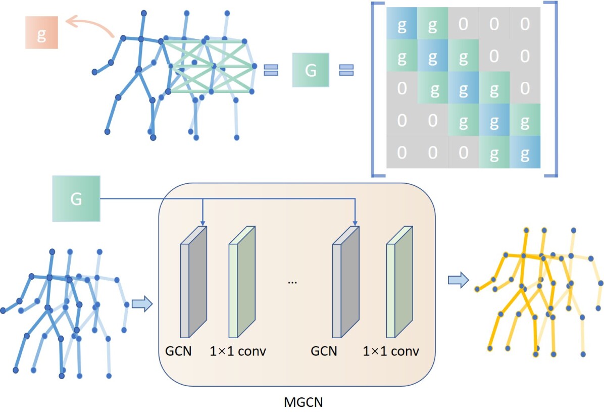
(a)

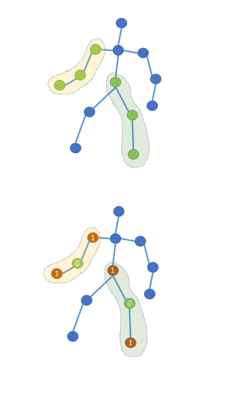
(b)

Figure 3: Overview of the MGCN model and Distance partition. For convenience, we assume that the human body has 13 joints. (a) illustrates the model MGCN. The graph G for MGCN consists of $T\times T$ g, where $T$ is the number of input frames. The blue parts show the connections inner frames; green parts show the connections inter frames; gray parts show the frames beyond time receptive field $L$. Here we illustrate the state when $T$ = 5, $L$ = 1. For every frame $t$, we merely connect from the frame $t-1$ to $t+1$ (if they exist). Given joints and G as input, MGCN outputs the prediction. (b) is the illustrations with or without Distance partition.

3.5 MGCN with sequence-aware attention

Many recent works on pose forecasting have used self-attention mechanisms to capture the relationship between frames [18, 4] and/or the relationship of joints [4]. We adopt the Multi-Graph Convolutional Network (MGCN) to produce the Query (Q), Key (K), and Value (V) representations. Due to the sequential nature of the data, we use masked attention which we refer it as sequence-aware attention. In contrast to using position encoding, which yielded suboptimal results, we propose two novel strategies for sequence-aware attention: Pseudo-autoregressive and Anchor.

Pseudo-autoregressive strategy: We directly set the $S$ matrix (see Figure 2) as a lower triangular matrix filled with 1. To achieve better results, we predict the coordinate offset of the original position instead of predicting the position directly. S * V achieves offset accumulation in the time dimension. The outputs are defined as follows:

$$offset=MGCN_{V}(X_{input},G)$$ (7)

$$X_{T+i}=\sum_{k=1}^{i}offset_{k}+X_{T},\quad offset_{k}\in\mathbb{R}^{V\times 3}.$$ (8)

The process of predicting future frames based on previous data is illustrated in Figure 4. This approach not only avoids the need to compute MGCN-Q and MGCN-K, but also achieves the best performance in short-term prediction (as discussed in more detail in Section 4.2).

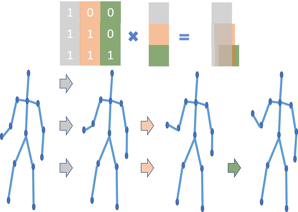
Figure 4: The illustration of the Pseudo-autoregressive strategy of sequence-aware attention. The output of time $t$ can be considered as a recursive addition of the previous offsets, so the model can have a global reception of movement.

Anchor (Possible Space): We introduce Anchor to add spatial constraints into our model. Firstly S matrix is generated by MGCN-Q and MGCN-K through masked softmax, and a set of anchors are produced by MGCN-V. The anchors work as a set of basis for Possible Space of future joints. Specially, it can be constructed as a cuboid along axis when there are only two anchors (Figure 5). Specifically, we use masked softmax on each of the three spatial dimensions (x, y, z), resulting in a reachable space that is a cuboid. The prediction for each joint is then a convex combination of these anchor points. The output in the frame $T+i$ is given by the following equation:

$$X_{T+i}^{d} =\sum_{k=1}^{i}\lambda_{ik}^{d}anchor_{k}^{d},\quad anchor_{k}\in\mathbb{R}^{V\times 3}$$ (9)

$$anchor=MGCN_{V}(X_{input},G),$$ (10)

where $\sum_{k=1}^{i}\lambda_{ik}^{d}=1$, $d\in{1,2,3}$. Figure 5 illustrates the process of predicting by 2 anchors. In our model, we use the 10 anchors to have a better understanding of the global movement.”

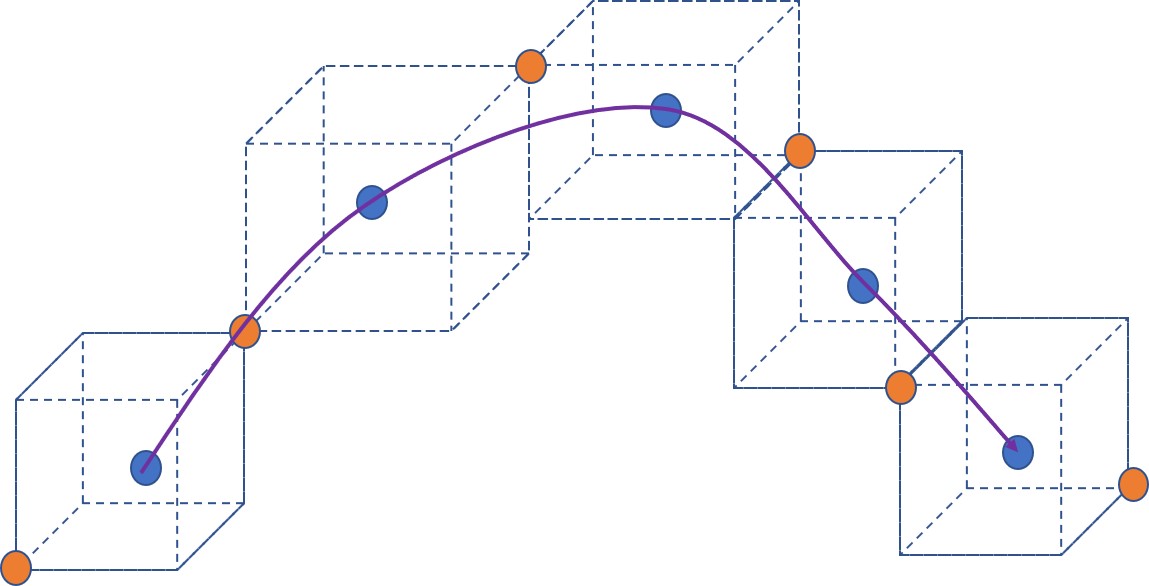
Figure 5: The illustration of the Anchor strategy. This strategy uses anchors to restrict the reachable space of the future joints. The yellow points on the corner of the cuboid are anchors, so the cuboid formed by two yellow anchors is the space where the future joint will be. We only use the last two anchors to form the reachable cuboid for the convenience of description.

3.6 TCN & Refine MGCN

The time dimension of the result after attention is same as the input (Equation 5). To fix the temporal mismatch between the output and target, we utilize Temporal Convolutional Networks to align the time dimension following [24]. Specifically, the 1*1 conv are applied in the temporal dimension.

Finally, a refined MGCN is used to improve the performance of the frame output.

msec	80	400	1000
DCT-RNN-GCN[18]	10.4	58.3	112.1
BGPIG[16]	10.3	58.5	-
STS-GCN[24]	10.1	38.3	75.6
SAA-10-MGCN L2D3	8.9	35.1	72.9
SAA-10-MGCN L6D4	8.6	34.4	83.6

Table 1: MPJPE error in mm for prediction of 3D joint positions on Human3.6M. All are given 10 frames to predict the 2, 10, 25 frames(80, 400, 1000 msec) in the future respectively. SAA-10-MGCN means the model using sequence-aware attention and 10 anchors before. L2D3 indicates we set L = 2, D = 3 in our MGCN. Our model outperforms the state-of-the-art on three scales. We change the temporal receptive field L and graph max hop distance D for different tasks.

	Walking				Eating				Smoking				Discussion
msec	80	160	320	400	80	160	320	400	80	160	320	400	80	160	320	400
DCT-RNN-GCN[18]	10.0	19.5	34.2	39.8	6.4	14.0	28.7	36.2	7.0	14.9	29.9	36.4	10.2	23.4	52.1	65.4
STS-GCN[24]	10.7	16.9	29.1	32.9	6.8	11.3	22.6	25.4	7.2	11.6	22.3	25.8	9.8	16.8	33.4	40.2
BGPIG[16]	10.2	19.8	34.5	40.3	7.0	15.1	30.6	38.1	6.6	14.1	28.2	34.7	10.0	23.8	53.6	66.7
Ours (L6D4)	9.3	14.0	24.7	28.6	5.7	10.2	18.9	22.3	5.8	10.9	20.0	22.9	8.0	14.6	29.8	35.9
	Directions				Greeting				Phoning				Posing
msec	80	160	320	400	80	160	320	400	80	160	320	400	80	160	320	400
DCT-RNN-GCN[18]	7.4	18.5	44.5	56.5	13.7	30.1	63.8	78.1	8.6	18.3	39.0	49.2	10.2	24.2	58.2	75.8
STS-GCN[24]	7.4	13.5	29.2	34.7	12.4	21.8	42.1	49.2	8.2	13.7	26.9	30.9	9.9	18.0	38.2	45.6
BGPIG[16]	7.2	17.6	40.9	51.5	15.2	34.1	71.6	87.1	8.3	18.3	38.7	48.4	10.7	25.7	60.0	76.6
Ours (L6D4)	5.9	11.5	24.5	30.6	10.8	18.3	35.9	44.5	6.8	12.5	23.1	27.7	7.7	15.5	32.4	40.9
	Purchases				Sitting				Sitting Down				Taking Photo
msec	80	160	320	400	80	160	320	400	80	160	320	400	80	160	320	400
DCT-RNN-GCN[18]	13.0	29.2	60.4	73.9	9.3	20.1	44.3	56.0	14.9	30.7	59.1	72.0	8.3	18.4	40.7	51.5
STS-GCN[24]	11.9	21.3	42.0	48.7	9.1	15.1	29.9	35.0	14.4	23.7	41.9	47.9	8.2	14.2	29.7	33.6
BGPIG[16]	12.5	28.7	60.1	73.3	8.8	19.2	42.4	53.8	13.9	27.9	57.4	71.5	8.4	18.9	42.0	53.3
Ours (L6D4)	10.2	18.6	37.1	44.2	7.6	14.1	26.6	31.8	14.0	21.7	37.8	45.5	7.0	13.3	25.4	30.9
	Waiting				Walking Dog				Walking Together				Average
msec	80	160	320	400	80	160	320	400	80	160	320	400	80	160	320	400
DCT-RNN-GCN[18]	8.7	19.2	43.4	54.9	20.1	40.3	73.3	86.3	8.9	18.4	35.1	41.9	10.4	22.6	47.1	58.3
STS-GCN[24]	8.6	14.7	29.6	35.2	17.6	29.4	52.6	59.6	8.6	14.3	26.5	30.5	10.1	17.1	33.1	38.3
BGPIG[16]	8.9	20.1	43.6	54.3	18.8	39.3	73.7	86.4	8.7	18.6	34.4	41.0	10.3	22.7	47.4	58.5
Ours (L6D4)	6.8	12.4	24.9	30.3	15.6	25.5	45.5	54.3	7.3	12.4	22.4	26.0	8.6	15.0	28.6	34.4

Table 2: MPJPE error in mm for short-term prediction of 3D joint positions on Human3.6M. Our model (L6D4) outperforms the state-of-the-art by a large margin. We use 10 frames (400 msec) as input and predict 2-10 frames(80-400 msec).

3.7 Training

In the MGCN architecture of end-to-end supervised training, we adopt the loss function based on Mean Per Joint Position Error (MPJPE)  [11, 19]

$${\cal L}_{MPJPE}=\frac{1}{V\times K}\sum_{k=T}^{T+K}\sum_{v=1}^{V}\left\|\hat{\boldsymbol{x}}_{v}^{k}-\boldsymbol{x}_{v}^{k}\right\|_{2},$$ (11)

where $\hat{\boldsymbol{x}}_{v}^{k}\in\mathbb{R}^{3}$ is the corresponding ground truth and $\boldsymbol{x}_{v}^{k}\in\mathbb{R}^{3}$ denotes the predicted coordinates of the joint $v$ in the $k$-th frame.

4 Experimental evaluation

We experimentally evaluate the proposed model against the state-of-the-art on the recent, large-scale and challenging benchmark, Human3.6M, AMASS and 3DPW.

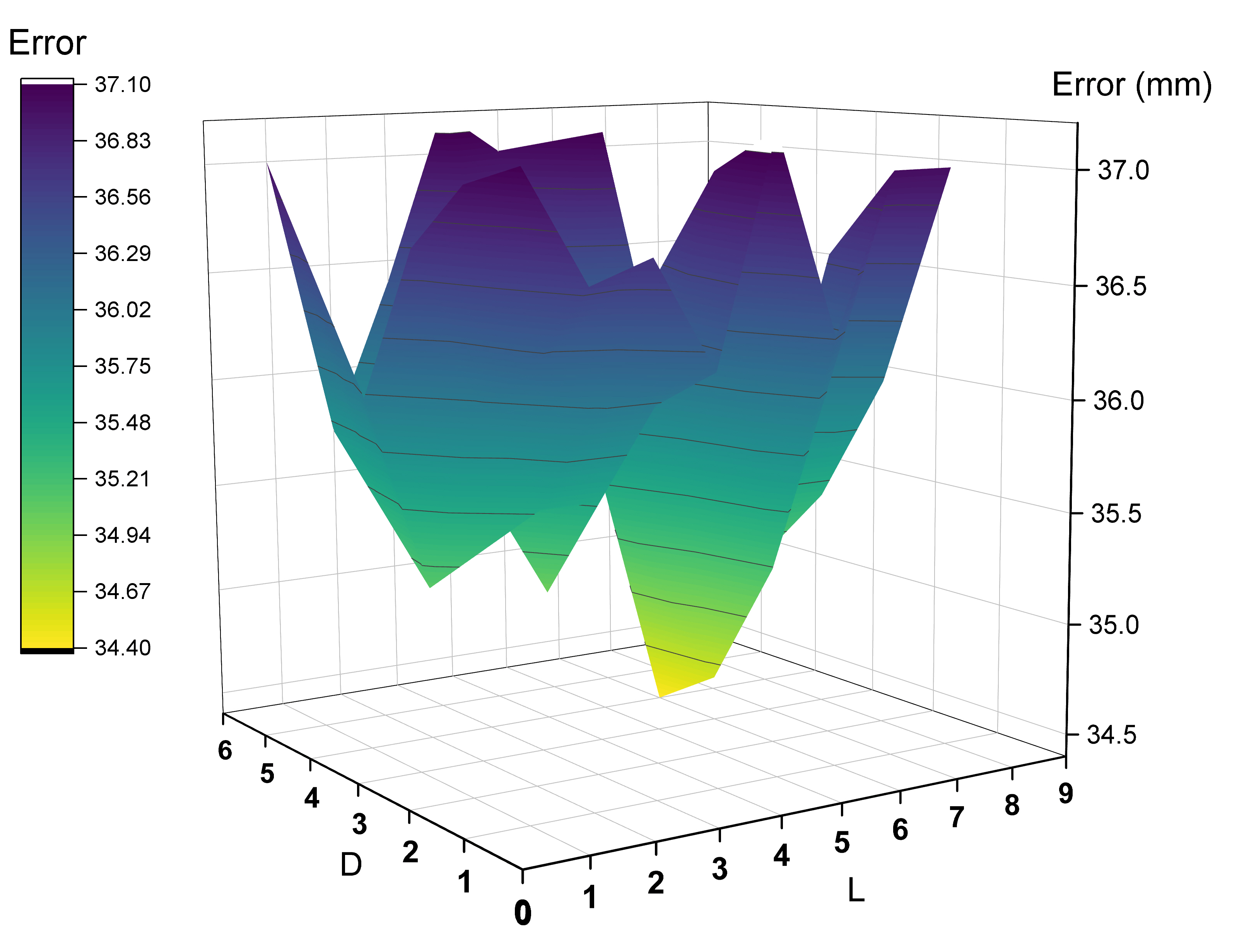
(a)

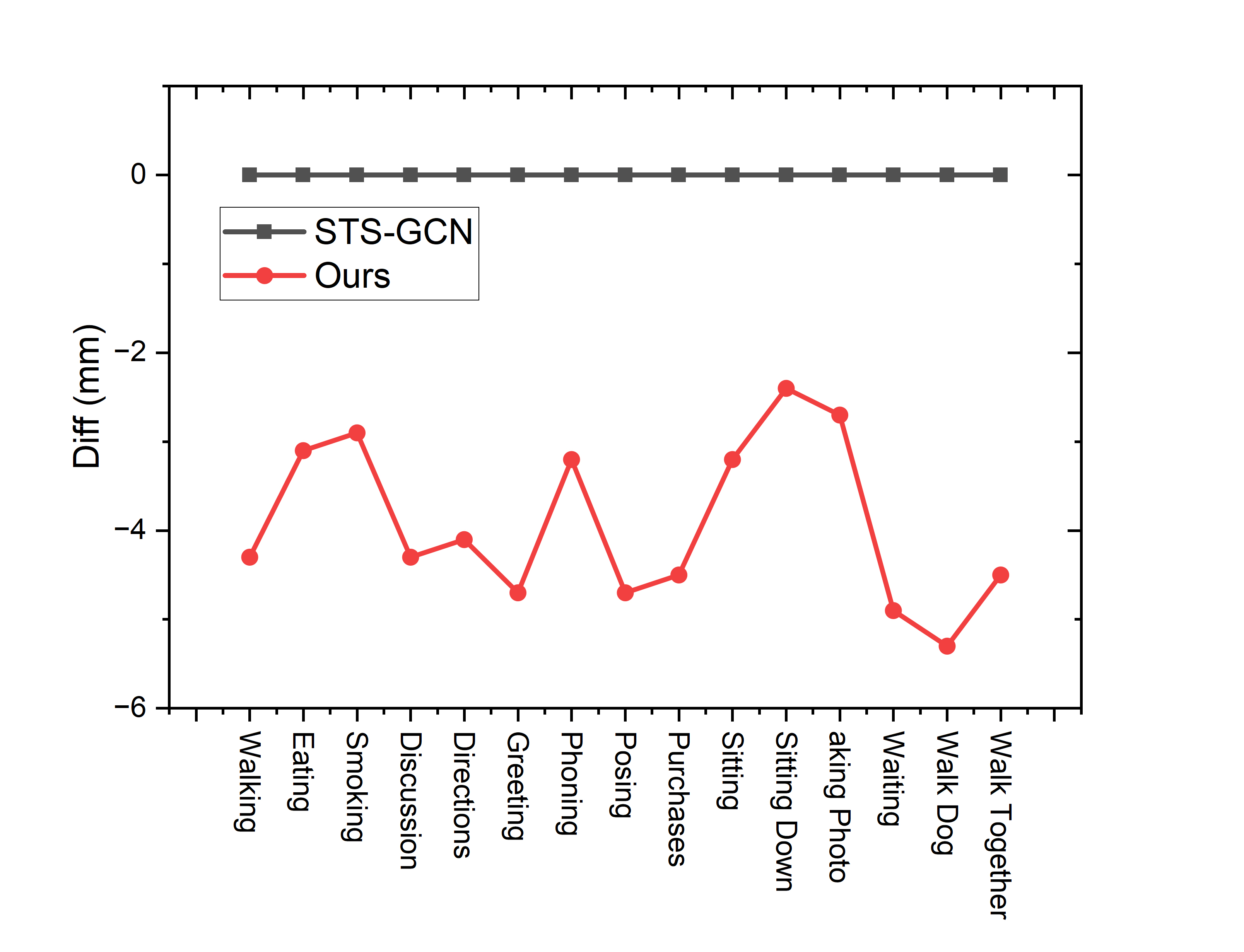
(b)

Figure 6: (a) The influence of hyperparameters L and D. The plot shows that the best performance of the model is obtained when L=4 and D=6 on 400ms task. (b)The advantage of our method is most significant for the action of “walking dog”.

4.1 Datasets and metrics

Human3.6M.[11] This dataset is widespread for human pose forecasting, which has 3.6 million 3D human poses and the corresponding images. It consists of 7 actors performing 15 different actions (e.g. Walking, Eating, Phoning). The actors are represented as skeletons of 32 joints. The orientations of joints are represented as exponential maps, from which the 3D coordinates may be computed [27, 9]. For each pose, we consider 22 joints out of the provided 32 for estimating MPJPE[24]. Following the current literature [19, 18, 20], we use the subject 11 (S11) for validation, the subject 5 (S5) for testing, and all the rest of the subjects for training.

AMASS[17] The Archive of Motion Capture as Surface Shapes (AMASS) dataset has been recently proposed, to gather 18 existing mocap datasets. We select 10 from those and take 5 for training, 4 for validation and 1 (BMLrub) as the test set. Then we use the SMPL [14] parameterization to derive a representation of human pose based on a shape vector and its joints rotation angles. We obtain human poses in 3D by applying forward kinematics. Overall, AMASS consists of 40 human-subjects that perform the action of walking. Each human pose is represented by 52 joints, including 22 body joints and 30 hand joints. Here we consider for forecasting the body joints only and discard from those 4 static ones, leading to an 18-joint human pose.

3DPW[31] The 3D Pose in the Wild dataset consists of video sequences acquired by a moving phone camera. 3DPW includes indoor and outdoor actions. Overall, it contains 51,000 frames captured at 30Hz, divided into 60 video sequences. We use this dataset to test generalization of the models trained on AMASS.

Metrics Following the benchmark protocols, we adopt the MPJPE error metrics. It quantifies the error of the 3D coordinate predictions in mm. We only adopted the 3D coordinate due to the inherent ambiguity of angle representation [4, 1].

Implementation details The MGCN is a seq2seq model which takes a series of joints from consecutive frames as inputs, and its outputs represent a series of vectors in the future consecutive frames. Following [24], we stack MGCN modules and only channel C changes: from 3 (the input dimension: x, y, z) to 64, then 32, 64, and finally 3. MGCN for Q and K change the channel by {3,64,32,16,16,3}. The masked softmax is adopted to implement sequence-aware attention. We train the model using the Adam optimizer on one NVIDIA RTX 2080Ti GPU with the minibatch size for GPU set as 256. The number of total epochs was fixed at 50. The learning rate is initially set to 0.1 and decays only at positions {20, 35, 45}.

	Walking				Eating				Smoking				Discussion
msec	560	720	880	1000	560	720	880	1000	560	720	880	1000	560	720	880	1000
DCT-RNN-GCN[18]	47.4	52.1	55.5	58.1	50.0	61.4	70.6	75.5	47.5	56.6	64.4	69.5	86.6	102.2	113.2	119.8
STS-GCN[24]	40.6	45.0	48.0	51.8	33.9	40.2	46.2	52.4	33.6	39.6	45.4	50.0	53.4	63.6	72.3	78.8
Ours (L2D3)	36.0	41.6	44.2	47.5	31.5	38.6	44.0	48.8	32.8	40.1	43.9	49.1	50.8	62.2	70.2	76.8
	Directions				Greeting				Phoning				Posing
msec	560	720	880	1000	560	720	880	1000	560	720	880	1000	560	720	880	1000
DCT-RNN-GCN[18]	73.9	88.2	100.1	106.5	101.9	118.4	132.7	138.8	67.4	82.9	96.5	105.0	107.6	136.8	161.4	178.2
STS-GCN[24]	47.6	56.5	64.5	71.0	64.8	76.3	85.5	91.6	41.8	51.1	59.3	66.1	64.3	79.3	94.5	106.4
Ours (L2D3)	44.1	54.7	63.6	69.9	60.8	73.2	83.9	89.3	40.0	50.1	56.6	63.9	60.2	75.8	89.8	100.3
	Purchases				Sitting				Sitting Down				Taking Photo
msec	560	720	880	1000	560	720	880	1000	560	720	880	1000	560	720	880	1000
DCT-RNN-GCN[18]	95.6	110.9	125.0	134.2	76.4	93.1	107.0	115.9	97.0	116.1	132.1	143.6	72.1	90.1	105.5	115.9
STS-GCN[24]	63.7	74.9	86.2	93.5	47.7	57.0	67.4	75.2	63.3	73.9	86.2	94.3	47.0	57.4	67.2	76.9
Ours (L2D3)	60.6	74.7	85.1	91.2	46.0	57.9	65.4	73.0	61.7	74.9	85.5	93.2	45.7	56.3	65.8	73.2
	Waiting				Walking Dog				Walking Together				Average
msec	560	720	880	1000	560	720	880	1000	560	720	880	1000	560	720	880	1000
DCT-RNN-GCN[18]	74.5	89.0	100.3	108.2	108.2	120.6	135.9	146.9	52.7	57.8	62.0	64.9	77.3	91.8	104.1	112.1
STS-GCN[24]	47.3	56.8	66.1	72.0	74.7	85.7	96.2	102.6	38.9	44.0	48.2	51.1	50.8	60.1	68.9	75.6
Ours (L2D3)	43.5	54.5	61.9	68.8	70.3	82.0	91.0	97.7	35.2	41.9	47.0	50.0	47.9	58.6	66.5	72.9

Table 3: MPJPE error in mm for short-term prediction of 3D joint positions on Human3.6M. Our model (L2D3) outperforms the state-of-the-art by a small margin. We use 10 frames (400 msec) as input and predict 14-25 frames(560-1000 msec).

msec	400
D = 4		L = 6
L = 2	35.1	D = 1	36.3
L = 3	35.5	D = 2	35.2
L = 4	35.0	D = 3	34.6
L = 5	35.5	D =4	34.4
L=6	34.4	D = 5	37.1
L = 7	34.8	D = 6	35.8
L = 10	35.2	D = 7	36.2
L=6, D=4	34.4

Table 4: The influence of temporal receptive field L and graph max hop distance D to MPJPE Error. In the first part, we fix the D = 4 and see the influence of L. In the second part, we fix the L = 6 and see the influence of D on the model.

msec	80	400	1000
no attention L2D3	9.1	35.8	74.4
attention L2D3	9.0	35.6	73.7
learnable graph L6D4	9.0	49.8	96.5
SAA-ar-MGCN L2D3	7.6	35.3	77.6
SAA-2-MGCN L2D3	8.5	36.0	77.8
SAA-10-no refine L2D3	9.1	36.1	76.4
SAA-10-no refine L6D4	9.0	35.3	82.2
SAA-10-MGCN L2D3	8.9	35.1	72.9
SAA-10-MGCN L6D4	8.6	34.4	83.6

Table 5: MPJPE error in mm for prediction of 3D joint positions on Human3.6M. All are given 10 frames to predict the 2, 10, 25 frames(80, 400, 1000 msec) in the future respectively. We experiment with the effects of the seq-attention mechanism, refine-MGCN, time receptive L and max hop D for the graph. No attention L2D3 means not using attention and setting L =2, D = 3, and attention L2D3 means using normal attention and setting L =2, D = 3.

msec	80	400	1000
H3.6M(STS-GCN[24])	10.1	38.3	75.6
H3.6M(our)	8.6	34.4	72.9
3DPW(STS-GCN[24])	8.6	24.5	42.3
3DPW(our)	8.1	24.0	40.3
AMASS(STS-GCN[24])	10.0	24.5	45.5
AMASS(our)	8.0	24.1	42.6

Table 6: Average MPJPE in mm. For the 80ms and 400ms prediction tasks, we set L=4 and D=6, while for the 1000ms prediction task, we set L=2 and D=3. In particular, for the experiments on AMASS and 3DPW datasets, we trained the model on AMASS and tested it on the BMLrub test sequences of both AMASS and 3DPW.

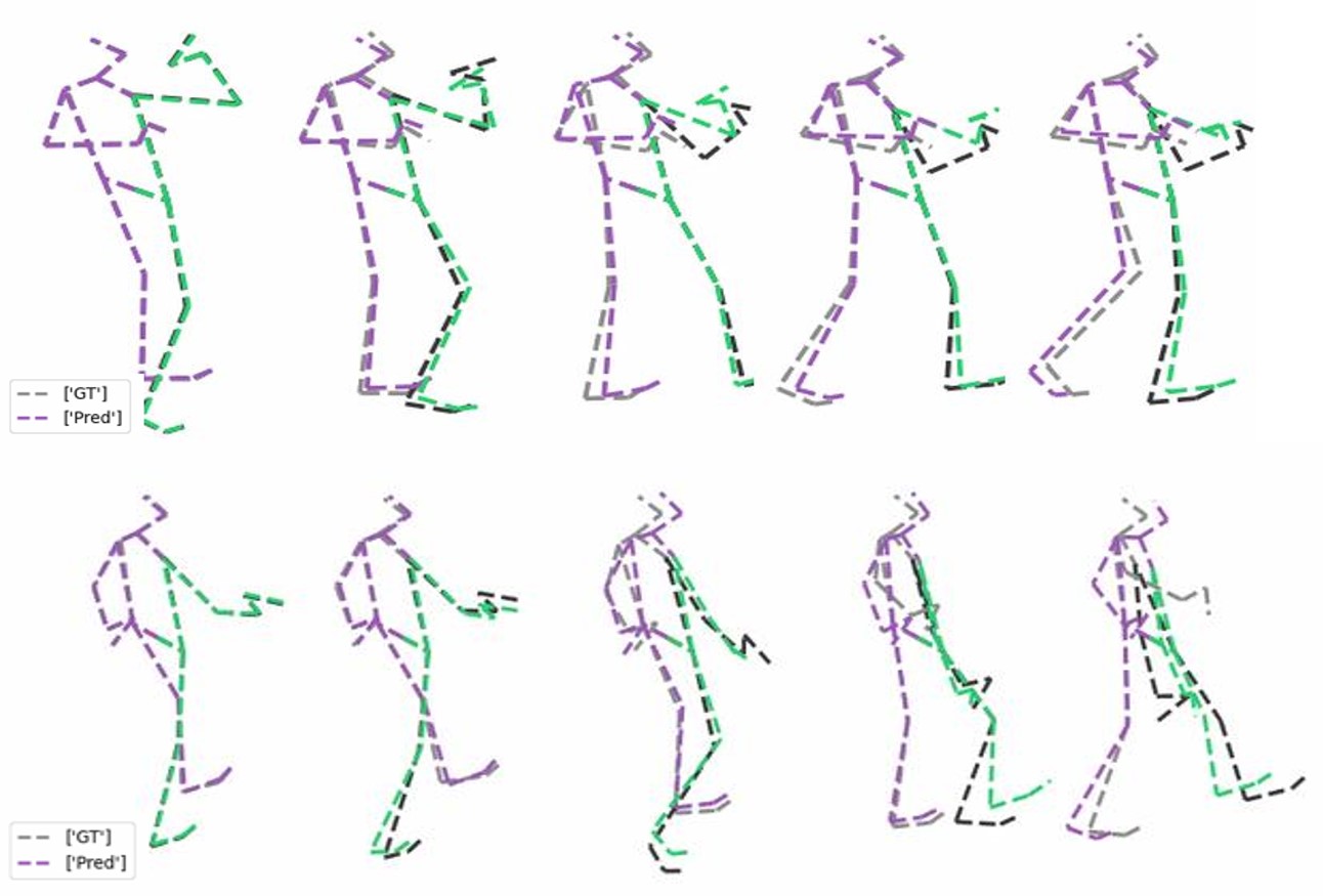
Figure 7: Sample long-term predictions (25 frames, 1 sec) for the actions of Eating and Walking. Purple/green limbs are the left/right sides of the body. Gray/black pictorials indicate the observed ground-truth (GT) skeletons.

4.2 Ablation study

Selection of L and D We conducted experiments to investigate how the temporal receptive field length (L) and the maximum hop distance in a graph (D) impact the performance of our model.

The Table 4 show that both L and D can negatively affect model performance if they are too short or too long. By comparing the "*-L2D3" and the "*-L6D4" models in Table 5, we found that the model with L6D4 outperformed the model with L2D3 for short-term prediction tasks.

Importance of natural link To explore the impact of the natural link on our model, we conduct experiments on the model with a learnable graph where all joints interconnected.

Comparing the "learnable graph L6D4" and "SAA-10-MGCN L6D4" models in Table 5, we observed a significant performance gap between the learnable graph and the natural link. This finding indicates that the natural connection plays a crucial role in human pose recognition.

Sequence-aware attention Comparing the "no attention L2D3" and "attention L2D3" models in Table 5, we found that models with attention outperformed those without attention on all prediction tasks. Furthermore, comparing the "attention L2D3" and "SAA-10-MGCN L2D3" models, sequence-aware attention performed better than normal attention. Comparing "SAA-2-MGCN L2D3" and "SAA-10-MGCN L2D3", more anchors benefit the score in long-term task. Notably, the "SAA-ar-MGCN" achieved the best performance on the 2 frames prediction task. It illustrates Pseudo-autoregressive strategy performance better than anchor strategy in 2 frames task. Therefore, we can choose different strategies for different problems to achieve the optimum.

Refine MGCN Comparing the last four models in Table 5, we observed that the "refine model" significantly improved the model’s performance for both short-term and long-term prediction tasks.

4.3 Other Findings and Discussion

Further analysis reveals predicting changeable movements, such as discussions, is more challenging than normal movements that typically involve periodic motion, like walking (See Table 2 and Table 3). Visual comparisons between our model and the ground truth are presented in Figure 7.

The results in Table 6 demonstrate that our proposed approach is effective and generalizable for different datasets. Our model achieved superior performance compared to state-of-the-art methods in terms of short-term and long-term predictions of 3D coordinates for both AMASS and 3DPW datasets. These results further validate the robustness and effectiveness of our proposed approach in predicting human poses over time.

GCN was adopted as a shape constraint model to avoid the physically impossible pose. Our MGCN extends this effect in the time dimension: GCN can constrain the structure, and MGCN can extra constrain the joint trajectory. GCN is a sort of fully connected network with prior information describing the connections, and if the graph is learnable, the topology information will be lost. We consider that the changeable motions are the most difficult task and may need to be offered more prior information like action category. And predicting movement from key points ignores important appearance features.

5 Conclusions

This paper has proposed a novel approach called multi-graph convolutional network (MGCN). The key to the effectiveness of the framework is that we simultaneously extract the spatial-temporal information and decompose the task into many steps. The proposed MGCN includes two attention strategies that make the model aware of the sequence, leading to state-of-the-art results on different tasks: 1) Pseudo-autoregressive strategy considers outputs as a recursive addition of the previous offsets; 2) Anchor strategy considers outputs as a convex combination of a set of anchors. Furthermore, by incorporating a post-processing step called Refine-MGCN, we were able to achieve significant improvements in the results. These findings provide further evidence for the superiority of our MGCN model. To build upon this approach, future work could consider applying it to other related problems such as human action recognition and pose interpolation.

References

- [1] Ijaz Akhter and Michael J. Black. Pose-conditioned joint angle limits for 3d human pose reconstruction. 2015 IEEE Conference on Computer Vision and Pattern Recognition (CVPR), pages 1446–1455, 2015.
- [2] Shaojie Bai, J. Zico Kolter, and Vladlen Koltun. An empirical evaluation of generic convolutional and recurrent networks for sequence modeling. ArXiv, abs/1803.01271, 2018.
- [3] Judith Bütepage, Michael J. Black, Danica Kragic, and Hedvig Kjellström. Deep representation learning for human motion prediction and classification. 2017 IEEE Conference on Computer Vision and Pattern Recognition (CVPR), pages 1591–1599, 2017.
- [4] Yujun Cai, Lin Huang, Yiwei Wang, T. Cham, Jianfei Cai, Junsong Yuan, Jun Liu, Xu Yang, Yiheng Zhu, Xiaohui Shen, Ding Liu, Jing Liu, and Nadia Magnenat-Thalmann. Learning progressive joint propagation for human motion prediction. In ECCV, 2020.
- [5] Hsu-kuang Chiu, Ehsan Adeli, Borui Wang, De-An Huang, and Juan Carlos Niebles. Action-agnostic human pose forecasting. In 2019 IEEE Winter Conference on Applications of Computer Vision (WACV), pages 1423–1432. IEEE, 2019.
- [6] Qiongjie Cui, Huaijiang Sun, and Fei Yang. Learning dynamic relationships for 3d human motion prediction. 2020 IEEE/CVF Conference on Computer Vision and Pattern Recognition (CVPR), pages 6518–6526, 2020.
- [7] Lingwei Dang, Yongwei Nie, Chengjiang Long, Qing Zhang, and Guiqing Li. Msr-gcn: Multi-scale residual graph convolution networks for human motion prediction. 2021 IEEE/CVF International Conference on Computer Vision (ICCV), pages 11447–11456, 2021.
- [8] Christian Diller, Thomas A. Funkhouser, and Angela Dai. Forecasting characteristic 3d poses of human actions. ArXiv, abs/2011.15079, 2020.
- [9] Katerina Fragkiadaki, Sergey Levine, Panna Felsen, and Jitendra Malik. Recurrent network models for human dynamics. 2015 IEEE International Conference on Computer Vision (ICCV), pages 4346–4354, 2015.
- [10] Jonas Gehring, Michael Auli, David Grangier, Denis Yarats, and Yann Dauphin. Convolutional sequence to sequence learning. In ICML, 2017.
- [11] Catalin Ionescu, Dragos Papava, Vlad Olaru, and Cristian Sminchisescu. Human3.6m: Large scale datasets and predictive methods for 3d human sensing in natural environments. IEEE Transactions on Pattern Analysis and Machine Intelligence, 36:1325–1339, 2014.
- [12] Hema Swetha Koppula and Ashutosh Saxena. Anticipating human activities for reactive robotic response. 2013 IEEE/RSJ International Conference on Intelligent Robots and Systems, pages 2071–2071, 2013.
- [13] Chen Li, Zhen Zhang, Wee Sun Lee, and Gim Hee Lee. Convolutional sequence to sequence model for human dynamics. 2018 IEEE/CVF Conference on Computer Vision and Pattern Recognition, pages 5226–5234, 2018.
- [14] Matthew Loper, Naureen Mahmood, Javier Romero, Gerard Pons-Moll, and Michael J. Black. Smpl: a skinned multi-person linear model. ACM Trans. Graph., 34:248:1–248:16, 2015.
- [15] Wenjie Luo, Binh Yang, and Raquel Urtasun. Fast and furious: Real time end-to-end 3d detection, tracking and motion forecasting with a single convolutional net. 2018 IEEE/CVF Conference on Computer Vision and Pattern Recognition, pages 3569–3577, 2018.
- [16] Tiezheng Ma, Yongwei Nie, Chengjiang Long, Qing Zhang, and Guiqing Li. Progressively generating better initial guesses towards next stages for high-quality human motion prediction. 2022 IEEE/CVF Conference on Computer Vision and Pattern Recognition (CVPR), pages 6427–6436, 2022.
- [17] Naureen Mahmood, Nima Ghorbani, Nikolaus F. Troje, Gerard Pons-Moll, and Michael J. Black. Amass: Archive of motion capture as surface shapes. 2019 IEEE/CVF International Conference on Computer Vision (ICCV), pages 5441–5450, 2019.
- [18] Wei Mao, Miaomiao Liu, and Mathieu Salzmann. History repeats itself: Human motion prediction via motion attention. In European Conference on Computer Vision, pages 474–489. Springer, 2020.
- [19] Wei Mao, Miaomiao Liu, Mathieu Salzmann, and Hongdong Li. Learning trajectory dependencies for human motion prediction. In Proceedings of the IEEE/CVF International Conference on Computer Vision, pages 9489–9497, 2019.
- [20] Julieta Martinez, Michael J. Black, and Javier Romero. On human motion prediction using recurrent neural networks. 2017 IEEE Conference on Computer Vision and Pattern Recognition (CVPR), pages 4674–4683, 2017.
- [21] Brian Paden, Michal Cáp, Sze Zheng Yong, Dmitry S. Yershov, and Emilio Frazzoli. A survey of motion planning and control techniques for self-driving urban vehicles. IEEE Transactions on Intelligent Vehicles, 1:33–55, 2016.
- [22] Razvan Pascanu, Tomas Mikolov, and Yoshua Bengio. On the difficulty of training recurrent neural networks. In ICML, 2013.
- [23] Chenyang Si, Wentao Chen, Wei Wang, Liang Wang, and Tieniu Tan. An attention enhanced graph convolutional lstm network for skeleton-based action recognition. 2019 IEEE/CVF Conference on Computer Vision and Pattern Recognition (CVPR), pages 1227–1236, 2019.
- [24] Theodoros Sofianos, Alessio Sampieri, Luca Franco, and Fabio Galasso. Space-time-separable graph convolutional network for pose forecasting. In Proceedings of the IEEE/CVF International Conference on Computer Vision, pages 11209–11218, 2021.
- [25] Chao Song, Youfang Lin, S. Guo, and Huaiyu Wan. Spatial-temporal synchronous graph convolutional networks: A new framework for spatial-temporal network data forecasting. In AAAI, 2020.
- [26] Yongyi Tang, Lin Ma, W. Liu, and Weishi Zheng. Long-term human motion prediction by modeling motion context and enhancing motion dynamic. ArXiv, abs/1805.02513, 2018.
- [27] Graham W. Taylor, Geoffrey E. Hinton, and Sam T. Roweis. Modeling human motion using binary latent variables. In NIPS, 2006.
- [28] Kalpit C. Thakkar and P. J. Narayanan. Part-based graph convolutional network for action recognition. ArXiv, abs/1809.04983, 2018.
- [29] Nikolaus F. Troje. Decomposing biological motion: a framework for analysis and synthesis of human gait patterns. Journal of vision, 2 5:371–87, 2002.
- [30] Ashish Vaswani, Noam M. Shazeer, Niki Parmar, Jakob Uszkoreit, Llion Jones, Aidan N. Gomez, Lukasz Kaiser, and Illia Polosukhin. Attention is all you need. ArXiv, abs/1706.03762, 2017.
- [31] Timo von Marcard, Roberto Henschel, Michael J. Black, Bodo Rosenhahn, and Gerard Pons-Moll. Recovering accurate 3d human pose in the wild using imus and a moving camera. In European Conference on Computer Vision, 2018.
- [32] Sijie Yan, Yuanjun Xiong, and Dahua Lin. Spatial temporal graph convolutional networks for skeleton-based action recognition. ArXiv, abs/1801.07455, 2018.
- [33] Ye Yuan and Kris Kitani. Ego-pose estimation and forecasting as real-time pd control. 2019 IEEE/CVF International Conference on Computer Vision (ICCV), pages 10081–10091, 2019.
- [34] Ye Yuan and Kris M. Kitani. Dlow: Diversifying latent flows for diverse human motion prediction. In ECCV, 2020.