On Beckner’s Inequality for Axially Symmetric Functions on $\mathbb{S}^{6}$

Abstract.

We prove that axially symmetric solutions to the $Q$-curvature type problem

$$\alpha P_{6}u+120(1-\frac{e^{6u}}{\int_{\mathbb{S}^{6}}e^{6u}})=0\ \ \ \ \ \mbox{on}\ \mathbb{S}^{6}$$

must be constants, provided that $\frac{1}{2}\leq\alpha<1$. In view of the existence of non-constant solutions obtained by Gui-Hu-Xie [17] for $\frac{1}{7}<\alpha<\frac{1}{2}$, this result is sharp. This result closes the gap of the related results in [17], which proved a similar uniqueness result for $\alpha\geq 0.6168$. The improvement is based on two types of new estimates: one is a better estimate of the semi-norm $\lfloor G\rfloor^{2}$, the other one is a family of refined estimates on Gegenbauer coefficients, such as pointwise decaying and cancellations properties.

1. Introduction and Main Results

Beckner’s inequality on $\mathbb{S}^{6}$, a higher order Moser-Trudinger inequality, asserts that the functional

$$J_{\alpha}(u):=\frac{\alpha}{2}\int_{\mathbb{S}^{6}}u(P_{6}u)\text{d}w+120\int_{\mathbb{S}^{6}}u\text{d}w-20\ln\int_{\mathbb{S}^{6}}e^{6u}\text{d}w$$

is non-negative for $\alpha=1$ and all $u\in H^{2}(\mathbb{S}^{6})$, where d$w$ denotes the normalized Lebesgue measure on $\mathbb{S}^{6}$ with $\int_{\mathbb{S}^{6}}\text{d}w=1$ and $P_{6}=-\Delta(-\Delta+4)(-\Delta+6)$ represents the Paneitz operator on $\mathbb{S}^{6}$. Additionally, with the extra assumption that the mass center of $u$ is at the origin and $u$ belongs to the set

$$\mathcal{L}=\left\{u\in H^{2}(\mathbb{S}^{6})\ :\ \int_{\mathbb{S}^{6}}e^{6u}x_{j}\text{d}w=0,\ j=1,...,7\right\},$$

an improved higher-order Moser-Trudinger-Onofri inequality demonstrates that for any $\alpha\geq\frac{1}{2}$, a constant $C(\alpha)\geq 0$ exists such that $J_{\alpha}(u)\geq-C(\alpha)$. As in the second-order case [7], it is conjectured that $C(\alpha)$ can be chosen to be $0$ for any $\alpha\geq\frac{1}{2}$.

The functional $J_{\alpha}$’s Euler-Lagrange equation is the following $Q$-curvature-type equation on $\mathbb{S}^{6}$

$$\alpha P_{6}u+120(1-\frac{e^{6u}}{\int_{\mathbb{S}^{6}}e^{6u}\text{d}w})=0\ \mbox{on}\ \mathbb{S}^{6},$$ (1.1)

If (1.1) admits only constant solutions, then the conjecture is valid. If $\alpha<1$ is near $1$, the third author and Xu [26] proved that all solutions to (1.1) are constants. However, for general $\alpha\in[\frac{1}{2},1)$, it remains unresolved. For results and backgrounds on $Q$-curvature problems, we refer to [9, 10, 11, 12, 16, 19, 21, 23, 26] and the references therein.

The corresponding problem on $\mathbb{S}^{2}$ is known as the Nirenberg problem:

$$-\alpha\Delta u+1-\frac{e^{2u}}{\int_{\mathbb{S}^{2}}e^{2u}}=0\ \ \mbox{on}\ \mathbb{S}^{2}.$$

This problem has been extensively studied over the past four decades. For more information, refer to [7, 8, 20] and the references therein. A. Chang and P. Yang conjectured in [7, 8] that the following functional

$$\alpha\int_{\mathbb{S}^{2}}|\nabla u|^{2}\text{d}w+2\int_{\mathbb{S}^{2}}u\text{d}w-\ln\int_{\mathbb{S}^{2}}e^{2u}\text{d}w$$

is non-negative for any $\alpha\geq\frac{1}{2}$ and $u$ with zero center of mass $\int_{\mathbb{S}^{2}}e^{2u}\vec{x}\text{d}w=0$. Feldman, Froese, Ghoussoub and the first author [13] demonstrated that the conjecture is true for axially symmetric functions when $\alpha>\frac{16}{25}-\epsilon$, the first and the third author in [18] confirmed that the conjecture is indeed true for axially symmetric functions. Later Ghoussoub and Lin [14] showed that the conjecture holds true for $\alpha>\frac{2}{3}-\epsilon$. Finally, the first author and Moradifam [15] proved the full conjecture. For more general results on improved Moser-Trudinger-Onofri inequality on $\mathbb{S}^{2}$ and its connections with the Szeg”o limit theorem, see [5, 6].

For the related problem on $\mathbb{S}^{4}$,

$$\alpha P_{4}u+6(1-\frac{e^{4u}}{\int_{\mathbb{S}^{4}}e^{4u}\text{d}w})=0\ \mbox{on}\ \mathbb{S}^{4},$$ (1.2)

various results have been achieved for axially symmetric solutions. Gui-Hu-Xie [16] proved the existence of non-constant solutions for $\frac{1}{5}<\alpha<\frac{1}{2}$ using bifurcation methods. They also demonstrated that for $\alpha\geq 0.517$, the above equation admits only constant solutions with axially symmetric assumption. The precise bound $\alpha\geq\frac{1}{2}$ is obtained by Li-Wei-Ye [22] using refined estimates on Gegenbauer polynomials.

These settings can be extended to the $\mathbb{S}^{n}$ case for any $n\geq 3$. Gui-Hu-Xie [17] established the existence of non-constant solutions using bifurcation methods for $\frac{1}{n+1}<\alpha<\frac{1}{2}$, while for $\alpha\geq 0.6168$ ($n=6$) and $\alpha\geq 0.8261$ ($n=8$), all critical points are constants.

In this paper, we focus on axially symmetric solutions in the $\mathbb{S}^{6}$ case for $\alpha\in[\frac{1}{2},1)$. As we will see later, the problem is considerably difficult.

As in [17], (1.1) becomes:

$$-\alpha[(1-x^{2})^{3}u^{\prime}]^{(5)}+120-128\frac{e^{6u}}{\gamma}=0,\ x\in(-1,1),$$ (1.3)

which is the critical point of the functional

$$I_{\alpha}(u) =-\frac{\alpha}{2}\int_{-1}^{1}(1-x^{2})^{2}[(1-x^{2})^{3}u^{\prime}]^{(5)}u+120\int_{-1}^{1}(1-x^{2})^{2}u$$

$$-\frac{64}{3}\ln\left(\frac{15}{16}\int_{-1}^{1}(1-x^{2})^{2}e^{6u}\right)$$ (1.4)

restricted to the set

$$\mathcal{L}_{r}=\{u\in H^{2}(\mathbb{S}^{6}):\ u=u(x)\text{ and }\int_{-1}^{1}x(1-x^{2})^{2}e^{6u}dx=0\}.$$ (1.5)

The main result of this paper is:

Theorem 1.1.

If $\alpha\geq\frac{1}{2}$, then the only critical points of the functional $I_{\alpha}$ restricted to $\mathcal{L}_{r}$ are constant functions. As a consequence, we have the following improved Beckner’s inequality for axially symmetric functions on $\mathbb{S}^{6}$

$$\inf_{u\in{\mathcal{L}_{r}}}I_{\alpha}(u)=0,\ \alpha\geq\frac{1}{2}.$$

In the work of Gui-Hu-Xie [17], the assumption $\alpha\geq\frac{1}{2}$ is shown to be sharp, and they proved Theorem 1.1 for $\alpha\geq 0.6168$ using a strategy similar to that in [16, 18, 22]. Specifically, they expand $G=(1-x^{2})u^{\prime}$ in terms of Gegenbauer polynomials and introduce a quantity $D$ related to the Gegenbauer coefficients and the estimate of $\lfloor G\rfloor^{2}$ (see (3)). However, unlike the $\mathbb{S}^{4}$ case discussed in [16], they are unable to obtain a bound on $\beta$ and, consequently, on $a=\frac{6}{7}(1-\alpha\beta)$. As a result, they cannot use $D$ to generate a series of inequalities as in [16] and proceed through the induction procedure.

In this paper, we provide a better estimate on $\lfloor G\rfloor^{2}$ and work with a revised quantity $D$. To render the induction procedure $a\leq\frac{d_{0}}{\lambda_{n}}$ feasible, we employ refined point-wise estimates of Gegenbauer polynomials similar to those in $\mathbb{S}^{4}$ [22] to improve the estimates of $G$’s Gegenbauer coefficients. More precisely, we refine the decaying behavior of Gegenbauer polynomials near $x=\pm 1$. Additionally, we utilize the cancellation properties of consecutive Gegenbauer polynomials to modify the methods in the $\mathbb{S}^{4}$ case.

This paper is organized as follows. In Section 2, we gather some properties of Gegenbauer polynomials, expand $G$ in terms of Gegenbauer polynomials, and cite some basic facts from [17]. In Section 3, we present improved estimates of $\lfloor G\rfloor^{2}$ and Gegenbauer coefficients of $G$. In Section 4, we prove Theorem 1.1 using the estimates above. Several Lemmas in Section 3 and Proposition 4.1 are proven in the appendices.

2. Preliminaries and some basic estimates

In this section, we first introduce some properties of Gegenbauer polynomials and some known facts about the equation.

The Gegenbauer polynomials of order $\nu$ and degree $k$ ([24]) is given by

$$C_{k}^{\nu}(x)=\frac{(-1)^{k}}{2^{k}k!}\frac{\Gamma(\nu+\frac{1}{2})\Gamma(k+2\nu)}{\Gamma(2\nu)\Gamma(\nu+k+\frac{1}{2})}(1-x^{2})^{-\nu+\frac{1}{2}}\frac{d^{k}}{dx^{k}}(1-x^{2})^{k+\nu-\frac{1}{2}}.$$

$C_{k}^{\nu}$ is an even function if $k$ is even and it is odd if $k$ is odd. The derivative of $C_{k}^{\nu}$ satisfies

$$\frac{d}{dx}C_{k}^{\nu}(x)=2\nu C_{k-1}^{\nu+1}(x).$$ (2.1)

Let $F_{k}^{\nu}$ be the normalization of $C_{k}^{\nu}$ such that $F_{k}^{\nu}(1)=1$, i.e.

$$F_{k}^{\nu}=\frac{k!\Gamma(2\nu)}{\Gamma(k+2\nu)}C_{k}^{\nu},$$ (2.2)

then $F_{k}^{\nu}$ satisfies

$$(1-x^{2})(F_{k}^{\nu})^{\prime\prime}-(2\nu+1)x(F_{k}^{\nu})^{\prime}+k(k+2\nu)F_{k}^{\nu}=0,$$ (2.3)

and (2.1) becomes

$$(F_{k}^{\nu})^{\prime}=\frac{k(k+2\nu)}{2\nu+1}F_{k-1}^{\nu+1}.$$ (2.4)

It is also useful to introduce the following expressions using hypergeometric functions

$$F_{2m+1}^{\nu}(\cos\theta)=\cos\theta{{}_{2}}F_{1}(-m,m+\nu+1;\nu+\frac{1}{2};\sin^{2}\theta),$$ (2.5)

$$F_{2m}^{\nu+1}(\cos\theta)={{}_{2}}F_{1}(-m,m+\nu+1;\nu+\frac{3}{2};\sin^{2}\theta),$$ (2.6)

where we recall the hypergeometric function is defined for $|x|<1$ by power series

$${{}_{2}}F_{1}(a,b;c;x)=\sum_{k=0}^{\infty}\frac{(a)_{k}(b)_{k}}{(c)_{k}}\frac{x^{k}}{k!}.$$

Here $(a)_{k}=\frac{\Gamma(a+k)}{\Gamma(a)}$ is the Pochhammer symbol.

On $\mathbb{S}^{6}$, the corresponding Gegenbauer polynomial is $C_{k}^{\frac{5}{2}}$. For notational simplicity, in what follows we will write $F_{k}$ for $F_{k}^{\frac{5}{2}}$, and there should be no danger of confusion.

From (2.3) it turns out that $F_{k}$ satisfies

$$(1-x^{2})F_{k}^{\prime\prime}-6xF_{k}^{\prime}+\lambda_{k}F_{k}=0$$ (2.7)

and

$$\int_{-1}^{1}(1-x^{2})F_{k}F_{l}=\frac{128}{(2k+5)(\lambda_{k}+4)(\lambda_{k}+6)}\delta_{kl},$$ (2.8)

where $\lambda_{k}=k(k+5)$. As in [16, 18], we define the following key quantity

$$G(x)=(1-x^{2})u^{\prime},$$ (2.9)

where $u$ is a solution to (1.3). Then $G$ satisfies the equation

$$\alpha[(1-x^{2})^{2}G]^{(5)}+120-128\frac{e^{6u}}{\gamma}=0,$$ (2.10)

where

$$\gamma=\int_{-1}^{1}(1-x^{2})^{2}e^{6u}.$$ (2.11)

$G$ can be expanded in terms of Gegenbauer polynomials

$$G=a_{0}F_{0}+\beta x+a_{2}F_{2}(x)+\sum_{k=3}^{\infty}a_{k}F_{k}(x).$$ (2.12)

Denote

$$g=(1-x^{2})^{2}\frac{e^{6u}}{\gamma},\ a:=\int_{-1}^{1}(1-x^{2})g.$$ (2.13)

We recall some results from [17].

Lemma 2.1.

For $g=(1-x^{2})^{2}\frac{e^{6u}}{\gamma}$ and $G=(1-x^{2})u^{\prime}$ as above, we have $a_{0}=0$ and

$$\int_{-1}^{1}(1-x^{2})F_{1}G=\frac{16}{105}\beta,$$ (2.14)

$$a=\int_{-1}^{1}(1-x^{2})g=\frac{6}{7}(1-\alpha\beta),$$ (2.15)

$$\int_{-1}^{1}(1-x^{2})F_{k}G=-\frac{128}{\alpha(\lambda_{k}+4)(\lambda_{k}+6)}\int_{-1}^{1}(1-x^{2})gF_{k}^{\prime},\text{ }k\geq 2,$$ (2.16)

$$\int_{-1}^{1}|[(1-x^{2})^{2}G]^{\prime\prime}|^{2}=\frac{256}{35}(7-\frac{1}{\alpha})\beta.$$ (2.17)

Lemma 2.2.

For all $x\in(-1,1)$, we have

$$G_{j}:=(-1)^{j}[(1-x^{2})^{j}G]^{(2j+1)}\leq\frac{(2j+1)!}{\alpha},\ 0\leq j\leq 2.$$ (2.18)

3. Refined Estimates

In this section, we deduce two refined estimates on the semi-norm $\lfloor G\rfloor^{2}$ and $b_{k}$ defined later.

To get a rough estimate of $\beta$ and $a=\frac{6}{7}(1-\alpha\beta)$, we need an estimate of the following semi-norm $\lfloor G\rfloor^{2}$. Let

$$\lfloor G\rfloor^{2}=-\int_{-1}^{1}(1-x^{2})^{2}[(1-x^{2})^{3}G^{\prime}]^{(5)}G.$$ (3.1)

By integrating by parts (see Gui-Hu-Xie [17]), we have

$$\lfloor G\rfloor^{2}= -15\int_{-1}^{1}|[(1-x^{2})^{2}G]^{\prime\prime}|^{2}+\frac{720}{\alpha}\int_{-1}^{1}(1-x^{2})^{2}G^{2}+30\int_{-1}^{1}(1-x^{2})^{4}G^{\prime}(G^{\prime\prime})^{2}$$

$$+160\int_{-1}^{1}(1-x^{2})^{3}(G^{\prime})^{3}.$$ (3.2)

With the help of Lemma 2.2, they applied $G^{\prime}\leq\frac{1}{\alpha}$ directly to the last two integrals and obtained an estimate of $\lfloor G\rfloor^{2}$

$$\lfloor G\rfloor^{2}\leq(\frac{30}{\alpha}-15)\int_{-1}^{1}|[(1-x^{2})^{2}G]^{\prime\prime}|^{2}-\frac{320}{\alpha}\int_{-1}^{1}(1-x^{2})^{3}(G^{\prime})^{2}.$$

However, with this estimate, it is not enough to get a rough lower bound of $\beta$, hence an upper bound of $a$. The main issue here is that the coefficient of $\int_{-1}^{1}|[(1-x^{2})^{2}G]^{\prime\prime}|^{2}$ is too large. To solve this problem, we introduce the following Proposition to drop the third integral in (3).

Proposition 3.1.

$$\lfloor G\rfloor^{2}\leq-15\int_{-1}^{1}|[(1-x^{2})^{2}G]^{\prime\prime}|^{2}+\frac{720}{\alpha}\int_{-1}^{1}(1-x^{2})^{2}G^{2}+\frac{160}{\alpha}\int_{-1}^{1}(1-x^{2})^{3}(G^{\prime})^{2},$$ (3.3)

Proof.

Integrating (3) by parts, we get

$$\lfloor G\rfloor^{2}= -15\int_{-1}^{1}|[(1-x^{2})^{2}G]^{\prime\prime}|^{2}+\frac{720}{\alpha}\int_{-1}^{1}(1-x^{2})^{2}G^{2}+\int_{-1}^{1}(1-x^{2})^{3}\tilde{G}(G^{\prime})^{2},$$

where

$$\tilde{G}=-15(1-x^{2})G^{\prime\prime\prime}+120xG^{\prime\prime}+160G^{\prime}.$$ (3.4)

Let

$$\hat{G}=-15(1-x^{2})G^{\prime\prime\prime}+120xG^{\prime\prime}+150G^{\prime}.$$ (3.5)

Direct calculation yields that $\hat{G}$ satisfies

$$(1-x^{2})\hat{G}^{\prime\prime}-8x\hat{G}^{\prime}-12\hat{G}=-15[(1-x^{2})^{2}G]^{(5)}\geq-\frac{1800}{\alpha}.$$

The last inequality follows from Lemma 2.2.

Then we claim that

$$\hat{G}\leq\frac{150}{\alpha}.$$

To prove the claim, denote $M=\max\limits_{-1\leq x\leq 1}\hat{G}(x)$.

If $M$ is attained at some point $x_{0}\in(-1,1)$, then

$$\hat{G}^{\prime}(x_{0})=0,\ \hat{G}^{\prime\prime}(x_{0})\leq 0$$

and the desired esitmate follows.

If $M$ is attained at $1$ or $-1$, without loss of generality, suppose there exists a sequence $x_{k}\to 1$ such that

$$M=\lim\limits_{k\to\infty}\hat{G}(x_{k}).$$

Let $r=\sqrt{1-x^{2}}$ and write

$$G(x)=\bar{G}(r)\text{ and }u(x)=\bar{u}(r)\text{ for }r\in[0,1),\ x\in(0,1].$$

Then we can extend $\bar{u}(r)$ to be a smooth even function on $(-\frac{1}{2},\frac{1}{2})$.

Hence,

$$G(x)=\bar{G}(r)=-r\sqrt{1-r^{2}}u_{r}$$

is a smooth function.

Direct calculation yields that

$$\hat{G}(r)=-15(1-r^{2})^{2}u_{rrrr}+30(1-r^{2})(7r^{2}-4)\frac{u_{rrr}}{r}-15(48r^{4}-50r^{2}+5)\frac{u_{rr}}{r^{2}}$$

is an even function with respect to $r$. Moreover, since

$$\lim\limits_{r\to 0}\frac{u_{rrr}(r)}{r}=u_{rrrr}(0),\ \lim\limits_{r\to 0}\frac{u_{rr}(r)}{r^{2}}=\frac{1}{2}u_{rrrr}(0),$$

$\hat{G}(r)$ is smooth on $(-\frac{1}{2},\frac{1}{2})$. Now we can write

$$\hat{G}(r) =c_{1}+c_{2}r^{2}+c_{3}r^{4}+O(r^{6}),$$

$$x\hat{G}^{\prime}(x) =-2c_{2}+O(r^{2}),$$

$$(1-x^{2})\hat{G}^{\prime\prime}(x) =(-2c_{2}+8c_{3})r^{2}+O(r^{4})$$

near $r=0$. Since $\hat{G}(r)$ attains its local maximum at $r=0$, we have $c_{2}\leq 0$ and hence

$$\lim\limits_{x\to 1}x\hat{G}^{\prime}(x)\leq 0,\ \lim\limits_{x\to 1}(1-x^{2})\hat{G}^{\prime\prime}(x)=0.$$

Then we obtain $M\leq\frac{150}{\alpha}$. Applying Lemma 2.2 again, we get

$$\tilde{G}\leq\frac{160}{\alpha}.$$

and the Proposition follows. ∎

In the following part, we begin to estimate $b_{k}:=a_{k}\sqrt{\int_{-1}^{1}(1-x^{2})F_{k}^{2}}$, where $a_{k}$ is the $k$-th coefficient in the expansion of $G$ (see (2.12)). The estimates of $b_{k}$ play a key role in the proofs of [16, 18]. In [16], they used (2.16) and the fact that

$$|F_{k}^{\prime}(x)|\leq|F_{k}^{\prime}(1)|=\frac{\lambda_{k}}{6}$$ (3.6)

to estimate $b_{k}$ as follows

$$b_{k}^{2} =a_{k}^{2}\int_{-1}^{1}(1-x^{2})F_{k}^{2}=\frac{1}{\int_{-1}^{1}(1-x^{2})F_{k}^{2}}\left[\frac{128}{\alpha\lambda_{k}}\int_{-1}^{1}(1-x^{2})gF_{k}^{\prime}\right]^{2}$$

$$\leq\frac{(2k+5)(\lambda_{k}+4)(\lambda_{k}+6)}{128}\left[\frac{128}{\alpha\lambda_{k}(\lambda_{k}+2)}\frac{\lambda_{k}}{6}a\right]^{2}$$

$$=\frac{32(2k+5)}{9\alpha^{2}(\lambda_{k}+4)(\lambda_{k}+6)}a^{2}.$$

However, as in the $\mathbb{S}^{4}$ case, this estimate is not strong enough to deduce the induction

$$a=\frac{6}{7}(1-\alpha\beta)\leq\frac{d_{0}}{\lambda_{n}}.$$ (3.7)

Likewise, we need a refined estimate on $b_{k}$, which follows from the following refined estimate on Gegenbauer polynomials. For simplicity, in the rest of the paper, we denote

$$\tilde{F}_{k}^{\prime}=\frac{6}{\lambda_{k}}F_{k}^{\prime}=\frac{720}{\lambda_{k}(\lambda_{k}+4)(\lambda_{k}+6)}C_{k-1}^{\frac{7}{2}}$$ (3.8)

so that $\tilde{F}_{k}^{\prime}(1)=1$. As in $\mathbb{S}^{4}$, we split the integral in the right hand side of $b_{k}$ into two parts. To this end, we define

$$a_{+}:=\int_{0}^{1}(1-x^{2})g,\ a_{-}:=\int_{-1}^{0}(1-x^{2})g,\ A_{k}^{+}=\int_{0}^{1}(1-x^{2})\tilde{F}_{k}^{\prime}g,\ A_{k}^{-}=\int_{-1}^{0}(1-x^{2})\tilde{F}_{k}^{\prime}g,$$ (3.9)

Without loss of generality, we may assume $a_{+}=\lambda a$ with $\frac{1}{2}\leq\lambda\leq 1$.

Now we derive some estimates about $g$. Recalling the definition of $g$, we have

$$\int_{-1}^{1}g=1,\ \int_{-1}^{1}xg=0\text{ and }\int_{-1}^{1}(1-x^{2})g=a.$$

From the second integral above, we have

$$\int_{0}^{1}g-\int_{0}^{1}(1-x)g=\int_{0}^{1}xg=-\int_{-1}^{0}xg=\int_{-1}^{0}g-\int_{-1}^{0}(1+x)g.$$ (3.10)

Since

$$\left|\int_{0}^{1}(1-x)g\right|\leq\int_{0}^{1}(1-x^{2})g=a_{+},\ \left|\int_{-1}^{0}(1+x)g\right|\leq\int_{0}^{1}(1-x^{2})g=a_{-},$$

combining with (3.10), we have

$$\left|\int_{0}^{1}g-\int_{-1}^{0}g\right|\leq a.$$

Hence

$$\frac{1-a}{2}\leq\int_{0}^{1}g,\int_{-1}^{0}g\leq\frac{1+a}{2}.$$ (3.11)

Moreover, it follows directly from the definition of $g$ that

$$\int_{0}^{1}xg\leq\min\{\int_{0}^{1}g,\int_{-1}^{0}g\}\leq\frac{1}{2},$$ (3.12)

and

$$\int_{0}^{1}(1+x)g=1-\int_{-1}^{0}(1+x)g<1.$$ (3.13)

With the estimates on $g$ above, the following Theorem gives a refined estimate on $A_{k}^{\pm}$, hence on $b_{k}$.

Theorem 3.2.

Let $d=8$, $b=0.33$. Suppose $a\leq\frac{16}{\lambda_{n}}$ for some $n\geq 3$. Then for all $k$, we have

$$|A_{k}^{+}|\leq\mathcal{A}_{k}^{+}:=\begin{cases}a_{+}-\frac{1-b}{d}\lambda_{k}a_{+}^{2},\text{ if }\lambda_{k}\leq\frac{\lambda_{n}}{4},\\ ba_{+}+(1-b)\frac{d}{4\lambda_{k}},\text{ if }\frac{\lambda_{n}}{4}<\lambda_{k}\leq\lambda_{n},\end{cases}$$ (3.14)

$$|A_{k}^{-}|\leq\mathcal{A}_{k}^{-}:=\begin{cases}a_{-}-\frac{1-b}{d}\lambda_{k}a_{-}^{2},\text{ if }a_{-}\leq\frac{4}{\lambda_{n}},\\ ba_{-}+(1-b)\frac{d}{4\lambda_{k}}\chi_{\{\lambda\neq 1\}},\text{ if }\frac{4}{\lambda_{n}}<a_{-}\leq\frac{8}{\lambda_{n}}.\end{cases}$$ (3.15)

In fact, for the toy cases in which $k$’s are small, better estimates can be obtained. The proof is left to Appendix A.

Lemma 3.3.

For $A_{k}$, $2\leq k\leq 5$,

$$|A_{2}| \leq a_{+}-a_{+}^{2},$$ (3.16)

$$|A_{3}| \leq a-\frac{9}{4}\frac{a^{2}}{a+1}(2\lambda^{2}-2\lambda+1),$$ (3.17)

$$|A_{4}| \leq (a_{+}-a_{+}^{2})-\frac{11}{4}(a_{+}-a_{+}^{2})^{2}+\frac{1}{4\sqrt{11}}a_{-},$$ (3.18)

$$|A_{5}| \leq a-\frac{11(a_{+}^{2}+a_{-}^{2})}{2(a+1)}+\frac{143(a_{+}^{3}+a_{-}^{3})}{10(a+1)^{2}}.$$ (3.19)

Before we prove Theorem 3.2 for general $k$’s, we first introduce some point-wise estimates of Gegenbauer polynomials.

Lemma 3.4 (Corollary 5.3 of Nemes and Olde Daalhuis [25] ).

Let $0<\zeta<\pi$ and $N\geq 3$ be an integer. Then

$$C_{k-1}^{\frac{7}{2}}(\cos{\zeta})=\frac{2}{\Gamma(\frac{7}{2})(2\sin{\zeta})^{\frac{7}{2}}}\left(\sum_{n=0}^{N-1}t_{n}(3)\frac{\Gamma(k+6)}{\Gamma(k+n+\frac{7}{2})}\frac{\cos{(\delta_{k-1,n})}}{\sin^{n}{\zeta}}+R_{N}(\zeta,k-1)\right),$$ (3.20)

where $\delta_{k,n}=(k+n+\frac{7}{2})\zeta-(\frac{7}{2}-n)\frac{\pi}{2}$, $t_{n}(\mu)=\frac{(\frac{1}{2}-\mu)_{n}(\frac{1}{2}+\mu)_{n}}{(-2)^{n}n!}$, and $(x)_{n}=\frac{\Gamma(x+n)}{\Gamma(x)}$ is the Pochhammer symbol. The remainder term $R$ satisfies the estimate

$$|R_{N}(\zeta,k)|\leq|t_{N}(3)|\frac{\Gamma(k+6)}{\Gamma(k+N+\frac{7}{2})}\frac{1}{\sin^{N}{\zeta}}\cdot\begin{cases}|\sec{\zeta}|&\text{ if }0<\zeta\leq\frac{\pi}{4}\text{ or }\frac{3\pi}{4}\leq\zeta<\pi,\\ 2\sin{\zeta}&\text{ if }\frac{\pi}{4}<\zeta<\frac{3\pi}{4}.\end{cases}$$ (3.21)

Using the pointwise estimate (3.20), we can prove the following lower and upper bounds for $\tilde{F}_{k}^{\prime}$. Recall that $\tilde{F}_{k}^{\prime}$ is odd for $k$ even and even for $k$ odd. It suffices to estimate $\tilde{F}_{k}^{\prime}$ on $[0,1]$. The proofs are left to Appendix B.

Lemma 3.5.

Let $m_{0}=0.04$, then for all $k\geq 8$, we have

$$\widetilde{F}_{k}^{\prime}\geq-m_{0},\quad 0\leq x\leq 1.$$

Lemma 3.6.

Let $d=8$ and $b=0.33$. Then for all $k\geq 6$,

$$\widetilde{F}_{k}^{{}^{\prime}}\leq\left\{\begin{aligned} &b,\quad&0\leq x\leq 1-\frac{d}{\lambda_{k}},\\ &1-\frac{\lambda_{k}}{d}(1-b)(1-x),\quad&1-\frac{d}{\lambda_{k}}\leq x\leq 1.\end{aligned}\right.$$

With the help of the above two lemmas, we are able to derive Theoreo 3.2.

Proof of Theorem 3.2.

By (4.4) below, we have $\beta\geq\frac{113}{88}$, $\alpha<0.578$ and hence $a\leq 0.221$. It is straightforward to check the cases when $2\leq k\leq 5$ hold for better estimate in the form of Lemma 3.6. In the following argument, we may assume $k\geq 6$. Define $I=(0,1-\frac{d}{\lambda_{k}})$, $II=(1-\frac{d}{\lambda_{k}},1)$, and $a_{I}=\int_{I}(1-x^{2})g$, $a_{II}=\int_{II}(1-x^{2})g$. Then by Lemma 3.6 and (3.13), we have

$$\int_{0}^{1}(1-x^{2})\widetilde{F}_{k}^{\prime}g =\int_{I}(1-x^{2})\widetilde{F}_{k}^{\prime}g+\int_{II}(1-x^{2})\widetilde{F}_{k}^{\prime}g$$

$$\leq\int_{I}(1-x^{2})bg+\int_{II}(1-x^{2})(1-\frac{\lambda_{k}}{d}(1-b)(1-x))g$$

$$=ba_{I}+a_{II}-\frac{\lambda_{k}}{d}(1-b)\int_{II}(1-x^{2})(1-x)g$$

$$\leq ba_{I}+a_{II}-\frac{\lambda_{k}}{d}(1-b)\frac{(\int_{II}(1-x^{2})g)^{2}}{\int_{II}(1+x)g}$$

$$\leq ba_{I}+a_{II}-\frac{\lambda_{k}}{d}(1-b)a_{II}^{2}$$

$$=ba_{+}+(1-b)(a_{II}-\frac{\lambda_{k}}{d}a_{II}^{2}).$$ (3.22)

If $\lambda_{k}\leq\frac{\lambda_{n}}{4}$, we have $a_{II}\leq a_{+}\leq a\leq\frac{16}{\lambda_{n}}\leq\frac{d}{2\lambda_{k}}$. Hence,

$$\int_{0}^{1}(1-x^{2})\widetilde{F}_{k}^{\prime}g\leq a_{+}+(1-b)(a_{+}-\frac{\lambda_{k}}{d}a_{+}^{2})=a_{+}-\frac{\lambda_{k}}{d}(1-b)a_{+}^{2}.$$

For the case when $\lambda_{k}>\frac{\lambda_{n}}{4}$, we get directly

$$\int_{0}^{1}(1-x^{2})\widetilde{F}_{k}^{\prime}g\leq ba_{+}+(1-b)\frac{d}{4\lambda_{k}}.$$

On the other hand, Lemma 3.5 yields

$$\int_{0}^{1}(1-x^{2})\widetilde{F}_{k}^{\prime}g\geq-0.04\int_{0}^{1}(1-x^{2})g=-0.04a_{+}.$$

Combining the above three estimates, we obtain the desired estimate on $A_{k}^{+}$.

Similarly, on estimating $A_{k}^{-}$, just note that $a_{-}\leq\frac{a}{2}\leq\frac{8}{\lambda_{n}}$. We can get an estimate analogous to (3.22) and then (3.15) follows directly. We omit the details. ∎

Next we derive a uniform estimate of cancellation of consecutive Gegenbauer polynomials. The estimate is based on the recursion formula and a useful inequality of Gegenbauer polynomials. It is well known that for $0<\nu<1$, $-1\leq x\leq 1$, one has

$$(1-x^{2})^{\frac{\nu}{2}}|C_{n}^{\nu}(x)|<\frac{2^{1-\nu}}{\Gamma(\nu)}n^{\nu-1},$$ (3.23)

where the constant $\frac{2^{1-\nu}}{\Gamma(\nu)}$ is optimal. (See Theorem 7.33.2 in [3]). We believe that an analogous result of (3.23) exists for $\nu>1$, but now the following lemma, whose proof is left to Appendix C, is enough for our use. We will use $F_{n}^{\nu}$ instead of $C_{n}^{\nu}$ for the sake of notational consistency.

Lemma 3.7.

For $\nu\geq 2$ and $-1\leq x\leq 1$, if $n\geq\max\{2\nu+2,12\}$, then we have

$$|(1-x^{2}){F}_{n}^{\nu}(x)|\leq\frac{\widetilde{C}_{\nu}}{n(n+2\nu)},$$ (3.24)

where $\widetilde{C}_{\nu}$ is given in(C.6).

With the help of the above lemma, we can prove the following proposition.

Proposition 3.8.

Let $c_{n}^{\nu}=\max\limits_{0\leq x\leq 1}|{F}_{n+1}^{\nu}(x)-{F}_{n}^{\nu}(x)|$. For $\nu\geq 2$, we have

$$c_{n}^{\nu}\leq\frac{1}{n}\left(\frac{\widetilde{C}_{\nu}}{n+2\nu+1}+\widetilde{C}_{\nu+1}\right)$$

if $n\geq\max\{2\nu+2,12\}$.

Proof.

Recall the recursion formula for Gegenbauer polynomials

$$(1-x^{2})2\nu C_{n}^{\nu+1}=-(n+1)xC_{n+1}^{\nu}+(n+2\nu)C_{n}^{\nu},$$

which, in view of (2.2), can be rewritten as

$$(1-x^{2})(n+2\nu+1)F_{n}^{\nu+1}=-xF_{n+1}^{\nu}+F_{n}^{\nu}.$$

Then by (3.24),

$$|F_{n+1}^{\nu}(x)-F_{n}^{\nu}(x)| =|(1-x)F_{n+1}^{\nu}(x)-(1-x^{2})(n+2\nu+1)F_{n}^{\nu+1}(x)|$$

$$\leq|(1-x^{2})F_{n+1}^{\nu}(x)|+(n+2\nu+1)|(1-x^{2})F_{n}^{\nu+1}(x)|$$

$$\leq\frac{\widetilde{C}_{\nu}}{(n+1)(n+2\nu+1)}+\frac{(n+2\nu+1)\widetilde{C}_{\nu+1}}{n(n+2\nu+2)}$$

$$\leq\frac{1}{n}\left(\frac{\widetilde{C}_{\nu}}{n+2\nu+1}+\widetilde{C}_{\nu+1}\right).$$

∎

Recall that $\tilde{F}_{n}^{\prime}=F_{n-1}^{\frac{7}{2}}$, so we have

Corollary 3.9.

Let $c_{n}=\max\limits_{0\leq x\leq 1}|\tilde{F}_{n+1}^{\prime}-\tilde{F}_{n}^{\prime}|$, then $c_{n}\leq 0.12$ if $6\leq n\leq 29$ and $c_{n}<0.026$ if $n\geq 30$.

Proof.

Direct computation by Matlab shows that the first assertion holds, and $c_{n}<0.026$ for $30\leq n\leq 428$ (the computational results are recorded in a supplemental data file). For $n>428$, by (C.6), we have $\widetilde{C}_{\frac{7}{2}}\leq 9.19$ and $\widetilde{C}_{\frac{9}{2}}\leq 11.02$, so we can also deduce that

$$c_{n}=c_{n-1}^{\frac{7}{2}}\leq\frac{11.1}{n-1}<0.026.$$

∎

4. proof of main theorem for $\mathbb{S}^{6}$

In this section, we will prove Theorem 1.1 for $\mathbb{S}^{6}$ by induction argument, with the help of refined estimates on $b_{k}$’s.

We claim that $\beta=0$, which yields that $(1-x^{2})^{2}G$ is a linear function by (2.17). Since $G$ is bounded on $(-1,1)$, we get $G\equiv 0$ and we are done.

So it suffices to show that $\beta=0$. We will argue by contradiction. If $\beta\neq 0$, then $0<\beta<\frac{1}{\alpha}$ since $a=\int_{-1}^{1}(1-x^{2})g=\frac{6}{7}(1-\alpha\beta)>0$. It then suffices to show $a=0$. We will achieve this by proving

$$a=\frac{6}{7}(1-\alpha\beta)\leq\frac{d_{0}}{\lambda_{n}},\ \forall n\geq 5\text{ with }n\equiv 1\text{ (mod }4),$$ (4.1)

where $d_{0}=16$.

As in [18] and [22], we will prove (4.1) by induction.

To begin with, we introduce the quantity

$$D=\sum\limits_{k=3}^{\infty}\left[\lambda_{k}(\lambda_{k}+4)(\lambda_{k}+6)-(14-\frac{74}{9\alpha})(\lambda_{k}+4)(\lambda_{k}+6)-\frac{160}{\alpha}\lambda_{k}-\frac{720}{\alpha}\right]b_{k}^{2}.$$ (4.2)

Then by (2.17) and (3.3), we get

$$D= \lfloor G\rfloor^{2}-(14-\frac{74}{9\alpha})\int_{-1}^{1}|[(1-x^{2})^{2}G]^{\prime\prime}|^{2}-\frac{160}{\alpha}\int_{-1}^{1}(1-x^{2})^{3}(G^{\prime})^{2}$$

$$-\frac{720}{\alpha}\int_{-1}^{1}(1-x^{2})^{2}G^{2}+\frac{16}{105}(\frac{2080}{3\alpha}+960)\beta^{2}$$

$$\leq (\frac{74}{9\alpha}-29)\int_{-1}^{1}|[(1-x^{2})^{2}G]^{\prime\prime}|^{2}+\frac{16}{105}(\frac{2080}{3\alpha}+960)\beta^{2}$$

$$= \frac{256}{35}(\frac{74}{9\alpha}-29)(7-\frac{1}{\alpha})\beta+\frac{512}{7}(\frac{13}{9\alpha}+2)\beta^{2}.$$ (4.3)

Since $D\geq 0$, $\alpha\geq\frac{1}{2}$ and $0<\beta<\frac{1}{\alpha}$, we obtain

$$\beta\geq\frac{9}{440}(29-\frac{74}{9\alpha})(7-\frac{1}{\alpha})\geq\frac{113}{88},$$ (4.4)

and

$$\frac{256}{35}(\frac{74}{9\alpha}-29)(7-\frac{1}{\alpha})+\frac{512}{7}(\frac{13}{9\alpha}+2)\frac{1}{\alpha}\geq 0,$$ (4.5)

which implies that

$$\alpha<0.578.$$ (4.6)

On the other hand, fix any integer $n\geq 3$, we have

$$D= \sum\limits_{k=3}^{\infty}\left[\lambda_{k}(\lambda_{k}+4)(\lambda_{k}+6)-(14-\frac{74}{9\alpha})(\lambda_{k}+4)(\lambda_{k}+6)-\frac{160}{\alpha}\lambda_{k}-\frac{720}{\alpha}\right]b_{k}^{2}$$

$$\geq \sum\limits_{k=n+1}^{\infty}\left[\lambda_{n+1}-14+\frac{74}{9\alpha}-\frac{160\lambda_{n+1}+720}{(\lambda_{n+1}+4)(\lambda_{n+1}+6)\alpha}\right](\lambda_{k}+4)(\lambda_{k}+6)b_{k}^{2}$$

$$+\sum\limits_{k=3}^{n}\left[\lambda_{k}-14+\frac{74}{9\alpha}-\frac{160\lambda_{k}+720}{(\lambda_{k}+4)(\lambda_{k}+6)\alpha}\right](\lambda_{k}+4)(\lambda_{k}+6)b_{k}^{2}$$

$$\geq (\lambda_{n+1}-14+\frac{275}{63\alpha})\sum\limits_{k=n+1}^{\infty}(\lambda_{k}+4)(\lambda_{k}+6)b_{k}^{2}$$

$$+\sum\limits_{k=3}^{n}(\lambda_{k}-14+\frac{176}{63}\alpha)(\lambda_{k}+4)(\lambda_{k}+6)b_{k}^{2}$$

$$= \sum\limits_{k=3}^{n}(\lambda_{k}-\lambda_{n+1}-\frac{11}{7\alpha})(\lambda_{k}+4)(\lambda_{k}+6)b_{k}^{2}$$

$$+(\lambda_{n+1}-14+\frac{275}{63\alpha})\left[\frac{256}{35}(7-\frac{1}{\alpha})\beta-\frac{128}{7}\beta^{2}-360b_{2}^{2}\right].$$ (4.7)

Combining (4.3) and (4.7), we get

$$0\leq \frac{256}{35}(7-\frac{1}{\alpha})(\frac{27}{7\alpha}-15-\lambda_{n+1})\beta+\frac{128}{7}(\lambda_{n+1}-6+\frac{71}{7\alpha})\beta^{2}$$

$$+\frac{176}{63\alpha}(\lambda_{2}+4)(\lambda_{2}+6)b_{2}^{2}+\sum\limits_{k=2}^{n}(\lambda_{n+1}-\lambda_{k}+\frac{11}{7\alpha})(\lambda_{k}+4)(\lambda_{k}+6)b_{k}^{2}.$$ (4.8)

Then we can start the induction procedure to prove $a\leq\frac{16}{\lambda_{n}}$, for all $n\geq 5$ with $n\equiv 1\text{ (mod }4)$. Note that from (4.4) and (4.6), we already have $a\leq 0.221\leq\frac{16}{\lambda_{5}}$.

By induction, now we assume $a\leq\frac{16}{\lambda_{n}}$ for some $n\geq 5$ with $n\equiv 1\text{ (mod }4)$. Then we will show that $a\leq\frac{16}{\lambda_{n+4}}$. We argue by contradiction and suppose $a>\frac{16}{\lambda_{n+4}}$ on the contrary.

Let $B_{k}=\frac{9\alpha^{2}}{32}(\lambda_{n+1}-\lambda_{k}+\frac{11}{7\alpha})(2k+5)$, then for every even $k$, we have

$$\frac{9\alpha^{2}}{32}\left[(\lambda_{n+1}-\lambda_{k}+\frac{11}{7\alpha})(\lambda_{k}+4)(\lambda_{k}+6)b_{k}^{2}+(\lambda_{n+1}-\lambda_{k+1}+\frac{11}{7\alpha})(\lambda_{k+1}+4)(\lambda_{k+1}+6)b_{k+1}^{2}\right]$$

$$= B_{k}(\int_{-1}^{1}(1-x^{2})\tilde{F}_{k}^{\prime}g)^{2}+B_{k+1}(\int_{-1}^{1}(1-x^{2})\tilde{F}_{k+1}^{\prime}g)^{2}$$

$$= B_{k}\left[(\int_{0}^{1}(1-x^{2})\tilde{F}_{k}^{\prime}g)^{2}+(\int_{-1}^{0}(1-x^{2})\tilde{F}_{k}^{\prime}g)^{2}\right]+B_{k+1}\left[(\int_{0}^{1}(1-x^{2})\tilde{F}_{k+1}^{\prime}g)^{2}+(\int_{-1}^{0}(1-x^{2})\tilde{F}_{k+1}^{\prime}g)^{2}\right]$$

$$+ 2B_{k}\int_{0}^{1}(1-x^{2})\tilde{F}_{k}^{\prime}g\int_{-1}^{0}(1-x^{2})(\tilde{F}_{k}^{\prime}+\tilde{F}_{k+1}^{\prime})g+2B_{k+1}\int_{0}^{1}(1-x^{2})(\tilde{F}_{k+1}^{\prime}-\tilde{F}_{k}^{\prime})g\int_{-1}^{0}(1-x^{2})\tilde{F}_{k+1}^{\prime}g$$

$$+ 2(B_{k+1}-B_{k})\int_{0}^{1}(1-x^{2})\tilde{F}_{k}^{\prime}g\int_{-1}^{0}(1-x^{2})\tilde{F}_{k+1}^{\prime}g$$

$$:= R_{k,1}+R_{k,2}+R_{k,3}.$$

Recall the definition of $\mathcal{A}_{k}^{\pm}$ from Theorem 3.2. By Theorem 3.2, we have

$$R_{k,1} =B_{k}\left[(\int_{0}^{1}(1-x^{2})\tilde{F}_{k}^{\prime}g)^{2}+(\int_{-1}^{0}(1-x^{2})\tilde{F}_{k}^{\prime}g)^{2}\right]$$

$$+B_{k+1}\left[(\int_{0}^{1}(1-x^{2})\tilde{F}_{k+1}^{\prime}g)^{2}+(\int_{-1}^{0}(1-x^{2})\tilde{F}_{k+1}^{\prime}g)^{2}\right]$$

$$\leq B_{k}\left(|\mathcal{A}_{k}^{+}|^{2}+|\mathcal{A}_{k}^{-}|^{2}\right)+B_{k+1}\left(|\mathcal{A}_{k+1}^{+}|^{2}+|\mathcal{A}_{k+1}^{-}|^{2}\right).$$ (4.9)

Let $c_{k}$ be defined as in Corollary 3.9, then we have

$$|\int_{-1}^{0}(1-x^{2})(\tilde{F}_{k}^{\prime}+\tilde{F}_{k+1}^{\prime})g|\leq c_{k}a_{-}=c_{k}(1-\lambda)a,$$

$$|\int_{0}^{1}(1-x^{2})(\tilde{F}_{k+1}^{\prime}-\tilde{F}_{k}^{\prime})g|\leq c_{k}a_{+}=c_{k}\lambda a.$$

So

$$R_{k,2} =2B_{k}\int_{0}^{1}(1-x^{2})\tilde{F}_{k}^{\prime}g\int_{-1}^{0}(1-x^{2})(\tilde{F}_{k}^{\prime}+\tilde{F}_{k+1}^{\prime})g$$

$$+2B_{k+1}\int_{0}^{1}(1-x^{2})(\tilde{F}_{k+1}^{\prime}-\tilde{F}_{k}^{\prime})g\int_{-1}^{0}(1-x^{2})\tilde{F}_{k+1}^{\prime}g$$

$$\leq 2(B_{k}+B_{k+1})c_{k}\lambda(1-\lambda)a^{2}.$$ (4.10)

Finally by Lemma 3.5, we have

$$R_{k,3}\leq\left\{\begin{aligned} &2(B_{k+1}-B_{k})\lambda(1-\lambda)a^{2},&\text{ if }B_{k}\leq B_{k+1},\\ &2(B_{k}-B_{k+1})m_{0}(1-\lambda)a^{2},&\text{ if }B_{k+1}<B_{k}.\end{aligned}\right.$$ (4.11)

Now from (4), (4) and (4.11), we can get the estimate of each term in the summation in (4.7) for each even $k$.

$$\frac{9\alpha^{2}}{32}[(\lambda_{n+1}-\lambda_{k}+\frac{11}{7\alpha})(\lambda_{k}+4)(\lambda_{k}+6)b_{k}^{2}+(\lambda_{n+1}-\lambda_{k+1}+\frac{11}{7\alpha})(\lambda_{k+1}+4)(\lambda_{k+1}+6)b_{k+1}^{2}]$$

$$\leq B_{k}\left(|\mathcal{A}_{k}^{+}|^{2}+|\mathcal{A}_{k}^{-}|^{2}\right)+B_{k+1}\left(|\mathcal{A}_{k+1}^{+}|^{2}+|\mathcal{A}_{k+1}^{-}|^{2}\right)+2(B_{k}+B_{k+1})c_{k}\lambda(1-\lambda)a^{2}$$

$$+ \left\{\begin{aligned} &2(B_{k+1}-B_{k})\lambda(1-\lambda)a^{2},&\text{ if }B_{k}\leq B_{k+1},\\ &2(B_{k}-B_{k+1})m_{0}(1-\lambda)a^{2},&\text{ if }B_{k+1}<B_{k}.\end{aligned}\right.$$ (4.12)

Remark 4.1.

Note that this estimate is better than the one in $\mathbb{S}^{4}$ case. Cancellation of consecutive Gegenbauer polynomials is used in the proof.

The right hand side above can be viewed as a function $f_{k,a}(\lambda)$ of $\lambda=\frac{a_{+}}{a}$. The following Proposition yields that the worst case is $\lambda=1$. In particular, in this case, we can drop the small terms $R_{k,2}$ and $R_{k,3}$. The proof is left to Appendix D.

Proposition 4.1.

Suppose $a$ satisfies $\frac{d_{0}}{\lambda_{n+4}}\leq a\leq\frac{d_{0}}{\lambda_{n}}$ for some $n\geq 5$ with $n\equiv 1\text{ (mod }4)$ where $d_{0}=16$. Let $f_{k,a}(\lambda)$ be defined as above. Then for any $k$ even, we have for $n\geq 41$,
(1) If $\lambda_{k}\leq\frac{1}{4}\lambda_{n}$, then

$$f_{k,a}(\lambda)\leq f_{k,a}(1)=B_{k}(a-\frac{1-b}{d}\lambda_{k}a^{2})^{2}+B_{k+1}(a-\frac{1-b}{d}\lambda_{k+1}a^{2})^{2}.$$ (4.13)

(2) If $\frac{1}{4}\lambda_{n}<\lambda_{k}\leq\lambda_{n}$, then

$$f_{k,a}(\lambda)\leq f_{k,a}(1)=B_{k}(ba+(1-b)\frac{d}{4\lambda_{k}})^{2}+B_{k+1}(ba+(1-b)\frac{d}{4\lambda_{k+1}})^{2}.$$ (4.14)

For $5\leq n\leq 65,$ we have

(1) If $\lambda_{k}\leq\frac{1}{4}\lambda_{n}$, then

$$f_{k,a}(\lambda)\leq B_{k}(a-\frac{1-b}{d}\lambda_{k}a^{2})^{2}+B_{k+1}(a-\frac{1-b}{d}\lambda_{k+1}a^{2})^{2}+\frac{1}{2}(B_{k}+B_{k+1})c_{k}a^{2}.$$ (4.15)

(2) If $\frac{1}{4}\lambda_{n}<\lambda_{k}\leq\lambda_{n}$, then

$$f_{k,a}(\lambda)\leq B_{k}(ba+(1-b)\frac{d}{4\lambda_{k}})^{2}+B_{k+1}(ba+(1-b)\frac{d}{4\lambda_{k+1}})^{2}+\frac{1}{2}(B_{k}+B_{k+1})c_{k}a^{2}.$$ (4.16)

In the following, we will assume $n>10000$. The case when $n<10000$ is checked by Matlab and is left to Appendix E .

With the help of Proposition 4.1 and by plugging it into (4), we obtain

$$0\leq \frac{256}{35}(7-\frac{1}{\alpha})(\frac{27}{7\alpha}-15-\lambda_{n+1})\frac{1}{\alpha}(1-\frac{7}{6}a)+\frac{128}{7}(\lambda_{n+1}-6+\frac{71}{7\alpha})\frac{1}{\alpha^{2}}(1-\frac{7}{6}a)^{2}$$

$$+ \frac{176}{63}\alpha(\lambda_{2}+4)(\lambda_{2}+6)b_{2}^{2}$$

$$+ \frac{32}{9\alpha^{2}}\sum_{k=2}^{\frac{n-3}{2}}(\lambda_{n+1}-\lambda_{k}+\frac{11}{7\alpha})(2k+5)(1-\frac{1-b}{d}\lambda_{k}\frac{16}{\lambda_{n+4}})^{2}a^{2}$$

$$+ \frac{32}{9\alpha^{2}}\sum_{k=\frac{n-1}{2}}^{n}(\lambda_{n+1}-\lambda_{k}+\frac{11}{7\alpha})(2k+5)(ba+(1-b)\frac{d}{4\lambda_{k}})^{2}.$$

$$\leq -\frac{512}{7}(\lambda_{n+1}+\frac{51}{7})(1-\frac{7}{6}a)+\frac{512}{7}(\lambda_{n+1}+\frac{100}{7})(1-\frac{7}{6}a)^{2}+\frac{22528}{63\alpha}a^{2}$$

$$+ \frac{128}{9}\sum_{k=2}^{\frac{n-3}{2}}(\lambda_{n+1}-\lambda_{k}+\frac{22}{7})(2k+5)(1-\frac{1-b}{d}\lambda_{k}\frac{16}{\lambda_{n+4}})^{2}a^{2}$$

$$+ \frac{128}{9}\sum_{k=\frac{n-1}{2}}^{n}(\lambda_{n+1}-\lambda_{k}+\frac{22}{7})(2k+5)(ba+(1-b)\frac{d}{4\lambda_{k}})^{2}.$$

$$=: g_{n,1}(a)+g_{n,2}(a)+g_{n,3}(a)=g_{n}(a)$$ (4.17)

where $g_{n,1},g_{n,2}$ and $g_{n,3}$ are defined at the last equality.

For $g_{n,2}(a)$, we can decompose it into three summations

$$g_{n,2}(a)=\frac{128}{9}\left[S_{1}-\frac{34(1-b)}{d\lambda_{n+4}}S_{2}+\frac{289(1-b)^{2}}{d^{2}\lambda_{n+4}^{2}}S_{3}\right]a^{2},$$ (4.18)

where

$$S_{1}=\sum_{k=2}^{\frac{n-3}{2}}(\lambda_{n+1}-\lambda_{k}+\frac{11}{7\alpha})(2k+5)=\frac{7}{32}n^{4}+\frac{23}{8}n^{3}-\frac{115}{112}n^{2}-\frac{4265}{56}n-\frac{20075}{224},$$ (4.19)

$$S_{2} =\sum_{k=2}^{\frac{n-3}{2}}(\lambda_{n+1}-\lambda_{k}+\frac{11}{7\alpha})(2k+5)\lambda_{k}$$

$$=\frac{5}{192}n^{6}+\frac{1}{2}n^{5}+\frac{3611}{1344}n^{4}-\frac{9}{28}n^{3}-\frac{100207}{5376}n^{2}-\frac{1393237}{896}n-\frac{1040985}{1024},$$ (4.20)

$$S_{3} =\sum_{k=2}^{\frac{n-3}{2}}(\lambda_{n+1}-\lambda_{k}+\frac{11}{7\alpha})(2k+5)\lambda_{k}^{2}$$

$$=\frac{13}{3072}n^{8}+\frac{41}{384}n^{7}+\frac{1525}{1792}n^{6}+\frac{3011}{2688}n^{5}-\frac{48697}{3584}n^{4}-\frac{14917}{384}n^{3}$$

$$+\frac{1000525}{5376}n^{2}-\frac{1393237}{896}n-\frac{1040985}{1024}$$ (4.21)

For $g_{n,3}(a)$, direct calculation yields that

$$\sum_{k=\frac{n-1}{2}}^{n}(\lambda_{n+1}-\lambda_{k}+\frac{22}{7})(2k+5)(ba+(1-b)\frac{d}{4\lambda_{k}})^{2}$$

$$= b^{2}S_{4}a^{2}+2b(1-b)(\lambda_{n+1}+\frac{22}{7})\frac{d}{4}S_{5}a-2b(1-b)\frac{d}{4}S_{6}a+(1-b)^{2}\frac{d^{2}}{16}(\lambda_{n+1}+\frac{22}{7})S_{7}-(1-b)^{2}\frac{d^{2}}{16}S_{5},$$ (4.22)

where

$$S_{4} =\sum_{k=\frac{n-1}{2}}^{n}(\lambda_{n+1}-\lambda_{k}+\frac{22}{7})(2k+5)=\frac{9}{32}n^{4}+\frac{33}{8}n^{3}+\frac{2763}{112}n^{2}+\frac{3753}{56}n+\frac{15147}{224},$$ (4.23)

$$S_{5}=\sum_{k=\frac{n-1}{2}}^{n}\frac{2k+5}{\lambda_{k}}=\sum_{k=\frac{n-1}{2}}^{n}(\frac{1}{k}+\frac{1}{k+5})\geq 1.3863,$$ (4.24)

$$S_{6}=\sum_{k=\frac{n-1}{2}}^{n}(2k+5)=\frac{3}{4}n^{2}+\frac{9}{2}n+\frac{27}{4},$$ (4.25)

$$S_{7} =\sum_{k=\frac{n-1}{2}}^{n}\frac{2k+5}{\lambda_{k}^{2}}=\frac{1}{5}\sum_{k=\frac{n-1}{2}}^{n}(\frac{1}{k^{2}}-\frac{1}{(k+5)^{2}})$$

$$=\frac{1}{5}\left(\frac{3}{(n+1)^{2}}-\frac{1}{(n+2)^{2}}+\frac{3}{(n+3)^{2}}-\frac{1}{(n+4)^{2}}+\frac{3}{(n+5)^{2}}+\frac{4}{(n+7)^{2}}+\frac{4}{(n-1)^{2}}\right)$$

$$\leq\frac{3}{n^{2}}.$$ (4.26)

To get a contradiction, we need to show that $g_{n}(a)$ is negative for $\frac{16}{\lambda_{n+4}}<a<\frac{16}{\lambda_{n}}$. Direct computation gives that for $n>10000$ with $n\equiv 1\text{ (mod }4)$, we have the following three estimates

$$g_{n,1}(a)= -\frac{512}{7}(\lambda_{n+1}+\frac{51}{7})(1-\frac{7}{6}a)+\frac{512}{7}(\lambda_{n+1}+\frac{100}{7})(1-\frac{7}{6}a)^{2}+\frac{22528}{63\alpha}a^{2}$$

$$= \frac{512}{7}\left[7-\frac{7}{6}a\lambda_{n+1}-\frac{149}{6}a+\frac{49}{36}\lambda_{n+1}a^{2}+\frac{175}{9}a^{2}\right]+\frac{22528}{63\alpha}a^{2}$$

$$\leq \frac{512}{7}\left(7-\frac{56}{3}\frac{\lambda_{n+1}}{\lambda_{n+4}}-\frac{1192}{3\lambda_{n+4}}+\frac{3136}{9\lambda_{n}}+\frac{44800}{9\lambda{n}^{2}}\right)+\frac{91543}{\lambda_{n}^{2}}\leq-853.33,$$

$$g_{n,2}(a)= \frac{128}{9}\left[S_{1}-\frac{67}{25\lambda_{n+4}}S_{2}+\frac{4489}{2500\lambda_{n+4}^{2}}S_{3}\right]a^{2}$$

$$\leq \frac{128}{9}\left[\left(\frac{56n^{4}}{\lambda_{n}^{2}}+\frac{736n^{3}}{\lambda_{n}^{2}}+\frac{1840n^{2}}{\lambda_{n+4}^{2}}-\frac{136480n}{7\lambda_{n+4}^{2}}-\frac{160600}{7\lambda_{n+4}^{2}}\right)\right.$$

$$+ \left.\left(-\frac{268n^{6}}{15\lambda_{n+4}^{3}}-\frac{343n^{5}}{\lambda_{n+4}^{3}}-\frac{1843n^{4}}{\lambda_{n+4}^{3}}+\frac{221n^{3}}{\lambda_{n}^{3}}+\frac{51154n^{2}}{\lambda_{n}^{3}}+\frac{231234n}{\lambda_{n}^{3}}+\frac{40683}{\lambda_{n}^{3}}\right)\right.$$

$$+ \left.\left(\frac{1.94524n^{8}}{\lambda_{n}^{4}}+\frac{49.0797n^{7}}{\lambda_{n}^{4}}+\frac{391.18n^{6}}{\lambda_{n}^{4}}+\frac{515n^{5}}{\lambda_{n+4}^{4}}-\frac{6245n^{4}}{\lambda_{n+4}^{4}}-\frac{17856n^{3}}{\lambda_{n+4}^{4}}\right.\right.$$

$$- \left.\left.\frac{85550n^{2}}{\lambda_{n}^{4}}-\frac{714770n}{\lambda_{n}^{4}}-\frac{467298}{\lambda_{n+4}^{4}}\right)\right]$$

$$\leq 571.123,$$

$$g_{n,3}(a)= \frac{128}{9}\left[0.1089S_{4}a^{2}+\frac{2211}{2500}(\lambda_{n+1}+\frac{22}{7})S_{5}a-\frac{2211}{2500}S_{6}a+\frac{4489}{2500}(\lambda_{n+1}+\frac{22}{7})S_{7}-\frac{4489}{2500}S_{5}\right]$$

$$\leq \frac{128}{9}\left[\left(\frac{7.8408n^{4}}{\lambda_{n}^{2}}+\frac{115n^{3}}{\lambda_{n}^{2}}+\frac{688n^{2}}{\lambda_{n}^{2}}+\frac{1869n}{\lambda_{n}^{2}}+\frac{1886}{\lambda_{n}^{2}}\right)+19.6166\frac{\lambda_{n+1}+\frac{22}{7}}{\lambda_{n}}-\frac{10.6128n^{2}}{\lambda_{n+4}}\right.$$

$$+ \left.\frac{13467}{2500}\frac{\lambda_{n+1}+\frac{22}{7}}{n^{2}}-2.48923\right]$$

$$\leq 280.95.$$

Combining three estimates above, we found

$$0\leq g_{n}(a)\leq-853.33+571.123+280.95<-1.257<0,$$

for all $n>10000$ with $n\equiv 1\text{ (mod }4)$ and $\frac{16}{\lambda_{n+4}}<a\leq\frac{16}{\lambda_{n}}$, which is a contradiction. Consequently, we finish the proof of Theorem 1.1.

Appendix A proof of Lemma 3.3

In this appendix, we prove Lemma 3.3.

Proof of Lemma 3.3.

Define $A_{m,n}^{+}=\int_{0}^{1}x^{m}(1-x^{2})^{n}g$, $A_{m,n}^{-}=\int_{-1}^{0}|x|^{m}(1-x^{2})^{n}g$, and $A_{m,n}=A_{m,n}^{+}+A_{m,n}^{-}$. We begin with the estimate of $A_{2}$. By definition,

$$|A_{2}|=|\int_{-1}^{1}x(1-x^{2})g|\leq\max\left\{A_{1,1}^{+},A_{1,1}^{-}\right\}.$$

By Cauchy-Schwartz inequality and (3.13),

$$a_{+}-A^{+}_{1,1}=\int_{0}^{1}(1-x^{2})(1-x)g\geq\frac{(\int_{0}^{1}(1-x^{2})g)^{2}}{\int_{0}^{1}(1+x)g}\geq a_{+}^{2},$$

so

$$A^{+}_{1,1}\leq a_{+}-a_{+}^{2}.$$

Similarly,

$$A^{-}_{1,1}\leq a_{-}-a_{-}^{2}.$$

Since $a<1$ and we have assumed $\lambda\geq\frac{1}{2}$, we conclude that

$$|A_{2}|\leq a_{+}-a_{+}^{2}.$$

The estimate of $|A_{4}|$ is similar to that of $|A_{2}|$. By definition,

$$A_{4}=\int_{-1}^{1}(1-x^{2})g\widetilde{F}_{4}^{\prime}=\frac{1}{8}\int_{-1}^{1}(1-x^{2})(11x^{2}-3)xg=A_{1,1}-\frac{11}{8}A_{1,2}.$$

By Cauchy-Schwartz inequality and (3.12),

$$A_{1,2}\geq\frac{(A_{1,1}^{+})^{2}}{\int_{0}^{1}xg}\geq 2(A_{1,1}^{+})^{2},$$

so

$$A_{4}^{+}\leq A_{1,1}^{+}-\frac{11}{4}(A_{1,1}^{+})^{2}$$

On the other hand,

$$A_{4}^{+}\geq\frac{1}{8}\min_{0\leq x\leq 1}\{(11x^{2}-3)x\}\int_{0}^{1}(1-x^{2})g=-\frac{1}{4\sqrt{11}}a_{+}.$$

In the same way,

$$-(A_{1,1}^{-}-\frac{11}{4}(A_{1,1}^{-})^{2})\leq A_{4}^{-}\leq\frac{1}{4\sqrt{11}}a_{-}.$$

Since $\lambda\geq\frac{1}{2}$, we conclude that

$$|A_{4}|\leq A_{1,1}^{+}-\frac{11}{4}(A_{1,1}^{+})^{2}+\frac{1}{4\sqrt{11}}a_{-}\leq(a_{+}-a_{+}^{2})-\frac{11}{4}(a_{+}-a_{+}^{2})^{2}+\frac{1}{4\sqrt{11}}a_{-}.$$

The estimates of $A_{3}$ and $A_{5}$ are slightly different. For $A_{3}$, we write

$$A_{3}=\int_{-1}^{1}(1-x^{2})g\widetilde{F}_{3}^{\prime}=\frac{1}{8}\int_{-1}^{1}(1-x^{2})(9x^{2}-1)g=\frac{1}{8}(9A_{2,1}-a).$$

By Cauchy-Schwartz inequality and (3.11),

$$(A_{2,1}^{+})^{2} \leq\int_{0}^{1}(1-x^{2})^{2}g\int_{0}^{1}x^{4}g$$

$$\leq(a_{+}-A_{2,1}^{+})(\frac{a+1}{2}-a_{+}-A_{2,1}^{+}),$$

so

$$A_{2,1}^{+}\leq a_{+}-\frac{2a_{+}^{2}}{a+1}.$$ (A.1)

In the same way,

$$A_{2,1}^{-}\leq a_{-}-\frac{2a_{-}^{2}}{a+1}.$$

Hence,

$$A_{2,1}\leq a-\frac{2a_{+}^{2}+2a_{-}^{2}}{a+1}=a-\frac{2a^{2}}{a+1}(2\lambda^{2}-2\lambda+1).$$

Therefore

$$A_{3}\leq a-\frac{9}{4}\frac{a^{2}}{a+1}(2\lambda^{2}-2\lambda+1),$$

which, together with the definition of $A_{3}$, implies

$$|A_{3}|\leq\max\left\{a-\frac{9}{4}\frac{a^{2}}{a+1}(2\lambda^{2}-2\lambda+1),\frac{a}{8}\right\}=a-\frac{9}{4}\frac{a^{2}}{a+1}(2\lambda^{2}-2\lambda+1).$$

Finally, for $A_{5}$, we have

$$A_{5}=\frac{1}{80}\int_{-1}^{1}(1-x^{2})(3-66x^{2}+143x^{4})g=\frac{1}{80}(80a-143A_{2,2}-77A_{2,0}).$$

By Cauchy-Schwartz inequality and (3.11),

$$A_{2,2}^{+}\geq\frac{(A_{2,1}^{+})^{2}}{\int_{0}^{1}x^{2}g}\geq\frac{(A_{2,1}^{+})^{2}}{\frac{a+1}{2}-a_{+}},$$

so by (A.1),

$$A_{5}^{+} \leq\frac{1}{80}\big{(}80a_{+}-\frac{143(A_{2,1}^{+})^{2}}{\frac{a+1}{2}-a_{+}}-77(a_{+}-A_{2,1}^{+})\big{)}$$

$$\leq\frac{1}{80}\Big{(}3a_{+}-11(a_{+}-\frac{2a_{+}^{2}}{a+1})(\frac{26a_{+}}{a+1}-7)\Big{)}$$

$$=a_{+}-\frac{11a_{+}^{2}}{2(a+1)}+\frac{143a_{+}^{3}}{10(a+1)^{2}}.$$

Therefore

$$A_{5}\leq a-\frac{11(a_{+}^{2}+a_{-}^{2})}{2(a+1)}+\frac{143(a_{+}^{3}+a_{-}^{3})}{10(a+1)^{2}}.$$

On the other hand,

$$A_{5}\geq\frac{1}{80}\min_{-1\leq x\leq 1}\{3-66x^{2}+143x^{4}\}\int_{-1}^{1}(1-x^{2})g=-\frac{3}{52}a.$$

From (4.4) and the estimates of $|A_{2}|$ and $|A_{3}|$, we can deduce that $a<0.125$, so now it is not hard to see that

$$|A_{5}|\leq a-\frac{11(a_{+}^{2}+a_{-}^{2})}{2(a+1)}+\frac{143(a_{+}^{3}+a_{-}^{3})}{10(a+1)^{2}}.$$

Thus the proof of Lemma 3.3 is completed. ∎

Appendix B proof of Lemma 3.5 and 3.6

In this appendix we prove Lemma 3.5 and Lemma 3.6. The proofs are technical and make use of many quantitative properties of Gegenbauer polynomials.

Before we prove Lemma 3.5, we first state some general lemma about Gegenbauer polynomials. Denote by $x_{nk}(\nu)$, $k=1,\cdots,n$, the zeros of $C_{n}^{\nu}(x)$ enumerated in decreasing order, that is, $1>x_{n1}(\nu)>\cdots>x_{nn}(\nu)>-1$.

Lemma B.1 (Corollary 2.3 in Area et al.[1]).

For any $n\geq 2$ and for every $\nu\geq 1$, the inequality

$$x_{n1}(\nu)\leq\sqrt{\frac{(n-1)(n+2\nu-2)}{(n+\nu-2)(n+\nu-1)}}\cos(\frac{\pi}{n+1})$$ (B.1)

holds.

The next lemma is well-known and it is valid for many other orthogonal polynomials.

Lemma B.2 (Olver et al. [2]).

Denote by $y_{nk}(\nu)$, $k=0,1,\cdots,n-1,n$, the local maxima of $|C_{n}^{\nu}(x)|$ enumerated in decreasing order, then $y_{n0}(\nu)=1,y_{nn}(\nu)=-1$, and we have

1. $y_{nk}(\nu)=x_{n-1,k}(\nu+1),\ k=1,\cdots,n-1.$

2. $|C_{n}^{\nu}(y_{n0}(\nu))|>|C_{n}^{\nu}(y_{n1}(\nu))|>\cdots>|C_{n}^{\nu}(y_{n,[\frac{n+1}{2}]}(\nu))|.$

3. $(C_{n}^{\nu})^{(k)}(x)>0$ on $(x_{n1}(\nu),1)$ for all $k=0,1,\cdots,n.$

Proof of Lemma 3.5.

Direct computation by Matlab shows that the lemma holds for $8\leq k\leq 200$, so in what follows we may assume $k>200$. . By Lemma B.1 and (2.1), we know that the minimum of $\widetilde{F}_{k}^{\prime}$ on $[0,1]$ is achieved at the point

$$x_{k-2,1}(\frac{9}{2})\leq\sqrt{\frac{(k-3)(k+5)}{(k+\frac{3}{2})(k+\frac{1}{2})}}\cos(\frac{\pi}{k-1})<1-\frac{12.5}{k^{2}}.$$ (B.2)

Taking $N=4$ in Lemma 3.4, we obtain

$$\tilde{F}_{k}^{\prime}(\cos{\zeta})=F_{k-1}^{\frac{7}{2}}(\cos{\zeta}) =48\sqrt{\frac{2}{\pi}}\left(\sum_{m=0}^{3}t_{m}(3)\frac{\Gamma(k)}{\Gamma(k+m+\frac{7}{2})}\frac{\cos{(\delta_{k-1,m})}}{\sin^{m+\frac{7}{2}}{\zeta}}+\widetilde{R}\right),$$ (B.3)

where $\widetilde{R}$ satisfies

$$|\widetilde{R}|\leq t_{4}(3)\frac{\Gamma(k)}{\Gamma(k+\frac{15}{2})}(\sin{\zeta})^{-\frac{15}{2}}\cdot\begin{cases}\sec{\zeta}&\text{ if }0<\zeta\leq\frac{\pi}{4},\\ 2\sin{\zeta}&\text{ if }\frac{\pi}{4}<\zeta<\frac{\pi}{2},\end{cases}$$ (B.4)

the value of $t_{m}(3)$ for $0\leq m\leq 3$ are listed below:

$$t_{0}(3)=1,t_{1}(3)=\frac{35}{8},t_{2}(3)=\frac{945}{128},t_{3}(3)=\frac{3465}{1024},t_{4}(3)=-\frac{45045}{32768}.$$

Let $\sin{\zeta}=\frac{l}{k}$. Then by (B.2) we can assume $l\geq 5$. From (B.4) we know that if $l\leq\frac{k}{\sqrt{2}}$, then

$$|\widetilde{R}|\leq|t_{4}(3)|\frac{k^{\frac{15}{2}}\Gamma(k)}{l^{\frac{15}{2}}\Gamma(k+\frac{15}{2})}\frac{1}{\sqrt{1-\frac{l^{2}}{k^{2}}}}<\frac{1.5}{l^{\frac{15}{2}}\sqrt{1-\frac{l^{2}}{k^{2}}}};$$ (B.5)

while if $l>\frac{k}{\sqrt{2}}$, then

$$|\widetilde{R}|\leq 2|t_{4}(3)|\frac{k^{\frac{15}{2}}\Gamma(k)}{l^{\frac{15}{2}}\Gamma(k+\frac{9}{2})}<\frac{3(\sqrt{2})^{\frac{15}{2}}}{k^{\frac{15}{2}}}.$$ (B.6)

To get the desired lower bound, we shall use the following simple estimates.

$$\cos(x+\delta)=\cos x-\delta\sin(x+h\delta)\geq\cos x-|\delta|.$$ (B.7)

$$\zeta-\sin\zeta\leq(\frac{\pi}{2}-1)\sin^{3}{\zeta}\leq\sin^{3}{\zeta},\ 0<\zeta<\frac{\pi}{2}.$$ (B.8)

With the help of (B.7) and (B.8), we have

$$\cos{(\delta_{k-1,m})} =\cos{\left((k+\frac{5}{2}+m)\zeta-(\frac{7}{2}-m)\frac{\pi}{2}\right)}$$

$$=\cos\left((k+\frac{5}{2}+m)\frac{l}{k}+(k+\frac{5}{2}+m)(\zeta-\sin\zeta)-(\frac{7}{2}-m)\frac{\pi}{2}\right)$$

$$\geq\cos\left(l-(\frac{7}{2}-m)\frac{\pi}{2}\right)-\left((k+\frac{5}{2}+m)(\zeta-\sin\zeta)+(\frac{5}{2}+m)\frac{l}{k}\right)$$

$$\geq\cos\left(l-(\frac{7}{2}-m)\frac{\pi}{2}\right)-(3+m)\frac{l}{k}.$$ (B.9)

Therefore we have

$$\sum_{m=0}^{3}t_{m}(3)\frac{\Gamma(k)}{\Gamma(k+m+\frac{7}{2})}\frac{\cos{(\delta_{k-1,m})}}{\sin^{m+\frac{7}{2}}{\zeta}}=\sum_{m=0}^{3}t_{m}(3)\frac{k^{m+\frac{7}{2}}\Gamma(k)}{\Gamma(k+m+\frac{7}{2})}\frac{\cos{(\delta_{k-1,m})}}{l^{m+\frac{7}{2}}}$$

$$\geq \ \frac{k^{\frac{13}{2}}\Gamma(k)}{\Gamma(k+\frac{13}{2})}\sum_{m=0}^{3}t_{m}(3)\frac{(k+\frac{7}{2}+m)_{3-m}}{k^{3-m}l^{m+\frac{7}{2}}}\left(\cos\left(l-(\frac{7}{2}-m)\frac{\pi}{2}\right)-(3+m)\frac{l}{k}\right)$$

$$\geq \min\left\{(1-\frac{16}{k})\sum_{m=0}^{3}t_{m}(3)\frac{(k+\frac{7}{2}+m)_{3-m}}{k^{3-m}l^{m+\frac{7}{2}}}\left(\cos\left(l-(\frac{7}{2}-m)\frac{\pi}{2}\right)-(3+m)\frac{l}{k}\right),0\right\}.$$

Write

$$(1-\frac{16}{k})\sum_{m=0}^{3}t_{m}(3)\frac{(k+\frac{7}{2}+m)_{3-m}}{k^{3-m}l^{m+\frac{7}{2}}}\left(\cos\left(l-(\frac{7}{2}-m)\frac{\pi}{2}\right)-(3+m)\frac{l}{k}\right)=\sum_{i=0}^{4}E_{i},$$

where

$$E_{0}=\frac{1024l^{3}\cos\left(l+\frac{\pi}{4}\right)-1920l^{2}\cos\left(l-\frac{\pi}{4}\right)-840l\cos\left(l+\frac{\pi}{4}\right)-315\cos\left(l-\frac{\pi}{4}\right)}{1024l^{13/2}},$$

$$E_{1}=\frac{-3\left(512l^{3}+1280l^{2}-2304l^{2}\cos\left(l+\frac{\pi}{4}\right)+700l-1920l\cos\left(l-\frac{\pi}{4}\right)+770\cos\left(l+\frac{\pi}{4}\right)-315\right)}{512kl^{11/2}},$$

$$E_{2}=\frac{-10368l^{2}+11520l+15296l\cos\left(l+\frac{\pi}{4}\right)+64920\cos\left(l-\frac{\pi}{4}\right)-5775}{256k^{2}l^{9/2}},$$

$$E_{3}=\frac{-3\left(478l^{2}-2705l-231l\cos\left(l+\frac{\pi}{4}\right)-1980\cos\left(l-\frac{\pi}{4}\right)\right)}{8k^{3}l^{9/2}}$$

$$E_{4}=\frac{297(-7l+80)}{8k^{4}l^{7/2}}.$$

If $5\leq l\leq 6.5$, then $E_{0}\geq-0.0002$, $E_{1}\geq-0.00025$, $E_{2}\geq-1.5\times 10^{-5}$, $E_{3}\geq-10^{-7}$, $E_{4}\geq 0$. By (B.5), $|\widetilde{R}|\leq 8\times 10^{-6}$. Therefore from (B.3) we have

$$\tilde{F}_{k}^{\prime}(\cos{\zeta})\geq-48\sqrt{\frac{2}{\pi}}\times 0.005\geq-0.04.$$

If $l>6.5$, then $E_{0}\geq-0.00077$, $E_{1}\geq-0.0002$, $E_{2}\geq-10^{-5}$, $E_{3}\geq-10^{-7}$, $E_{4}\geq-10^{-9}$. Either (B.5) or (B.6) implies $|\widetilde{R}|\leq 3\times 10^{-7}$, so we also have

$$\tilde{F}_{k}^{\prime}(\cos{\zeta})\geq-48\sqrt{\frac{2}{\pi}}\times 0.01\geq-0.04.$$

Thus the lemma is proved. ∎

Proof of Lemma 3.6.

We first prove the following estimate at one point:

$$0.3\leq\tilde{F}_{k}^{\prime}(1-\frac{8}{\lambda_{k}})\leq 0.33,\quad k\geq 6.$$ (B.10)

Direct computation by Matlab shows that (B.10) holds for $6\leq k\leq 100$, so in what follows we may assume $k>100$. The main tool we use is the hypergeometric expansion (2.5) and (2.6). We will prove (B.10) only for even $k$, and the case for odd $k$ is similar.

Let $k=2m+2$, then $\tilde{F}_{k}^{\prime}=F_{k-1}^{\frac{7}{2}}$, so by (2.5),

$$\tilde{F}_{k}^{\prime}(1-\frac{8}{\lambda_{k}})=(1-\frac{8}{\lambda_{k}}){{}_{2}}F_{1}(-m,m+\frac{9}{2};4;t),$$

where $t=1-(1-\frac{8}{\lambda_{k}})^{2}=\frac{8}{\lambda_{k}}(2-\frac{8}{\lambda_{k}})$. Now we write

$${{}_{2}}F_{1}(-m,m+\frac{9}{2};4;t)=\sum_{i=0}^{m}(-1)^{i}\gamma_{i}t^{i},$$

where $\gamma_{i}=\frac{(m-i+1)_{i}(m+\frac{7}{2})_{i}}{i!(4)_{i}}$. It is easy to see that

$$\min\limits_{1\leq i<m}\{\frac{\gamma_{i}}{\gamma_{i+1}}\}=\frac{\gamma_{1}}{\gamma_{2}}=\frac{10}{(m-1)(m+\frac{9}{2})}=\frac{40}{(k-3)(k+7)}>t.$$

Therefore

$$\sum_{i=0}^{j_{1}\text{ is odd}}(-1)^{i}\gamma_{i}t^{i}\leq{{}_{2}}F_{1}(-m,m+\frac{9}{2};4;t)\leq\sum_{i=0}^{j_{2}\text{ is even}}(-1)^{i}\gamma_{i}t^{i}$$

Take $j_{1}=5,j_{2}=6$, then direct computation shows that (B.10) holds since $m\geq 50$.

Now in view of Lemma 3.5, we see that $\tilde{F}_{k}^{\prime}(1-\frac{8}{\lambda_{k}})>-\min\limits_{0\leq x\leq 1}\tilde{F}_{k}^{\prime}(x)$. Then by Lemma B.2 $(b)$, $\tilde{F}_{k}^{\prime}(1-\frac{8}{\lambda_{k}})\geq\tilde{F}_{k}^{\prime}(x)$ for all $0\leq x\leq 1-\frac{8}{\lambda_{k}}$. Moreover, the convexity of $\widetilde{F}_{k}^{\prime}(x)$ on $[1-\frac{8}{\lambda_{k}},1]$ is guaranteed by Lemma B.2 $(c)$. This completes the proof of Lemma 3.6. ∎

Appendix C proof of Lemma 3.7

We first prove a simple lemma, which enables us to focus on the region near $x=1$. By letting $x=\cos\theta$, we introduce the function $v(\theta)=(\sin\theta)^{2}F_{n}^{\nu}(\cos\theta)$ in this appendix.

Lemma C.1.

For $n\geq 2$ and $\nu>0$, let $v(\theta)$ be defined as above. If $\nu\geq 2$, then the successive relative maxima of $|v(\theta)|$ form an increasing sequence as $\theta$ decreases from $\frac{\pi}{2}$ to $0$.

Proof of Lemma C.1.

By (2.3) it is straightforward to check that $v$ satisfies the equation

$$v^{\prime\prime}(\theta)+p(\theta)v^{\prime}(\theta)+q(\theta)=0,$$

where $p(\theta)=(2\nu-4)\cos\theta$, and $q(\theta)=(n^{2}+2\nu n+4)-\frac{2}{\sin^{2}\theta}+(4\nu-8)(\sin\theta-\frac{1}{\sin\theta})$. Since $\nu>2$, we know that $p\geq 0$, $q$ is increasing and $q$ has a unique zero $\widetilde{\theta}$ in $(0,\frac{\pi}{2})$ .

Since $v(0)=0,v^{\prime}>0$ near $0$, and $q(\theta)<0$ in $(0,\widetilde{\theta})$, by the maximum principle, it’s easy to see that $|v(\theta)|$ has no local maxima in $(0,\widetilde{\theta}]$. Now we consider the case when $\theta\in(\widetilde{\theta},\frac{\pi}{2}]$. Let $\tilde{q}=q^{-1}$, then $\tilde{q}>0$ is strictly decreasing in $(\widetilde{\theta},\frac{\pi}{2}]$. Introducing

$$f(\theta)=v^{2}(\theta)+\tilde{q}(\theta)(v^{\prime})^{2}(\theta),$$

we have

$$f^{\prime}=\tilde{q}^{\prime}(v^{\prime})^{2}+2v^{\prime}(\tilde{q}v^{\prime\prime}+v)=(\tilde{q}^{\prime}-2p\tilde{q})u^{\prime 2}<0.$$

But $f(\theta)=v^{2}(\theta)$ if $v^{\prime}(\theta)=0$, so the lemma is proved. ∎

Proof of Lemma 3.7.

In view of Lemma C.1, we need to find a bound for $\theta_{*}$, the smallest zero of $v^{\prime}(\theta)$ in $(0,\frac{\pi}{2})$. By definition of $v$ and (2.4),

$$v^{\prime}(\theta) =\sin\theta\left(2\cos\theta F_{n}^{\nu}(\cos\theta)-\sin^{2}\theta(F_{n}^{\nu})^{\prime}(\cos\theta)\right)$$

$$=\sin\theta\left(2\cos\theta F_{n}^{\nu}(\cos\theta)-\frac{n(n+2\nu)}{2\nu+1}\sin^{2}\theta F_{n-1}^{\nu+1}(\cos\theta)\right).$$

We claim that when $\theta=\overline{\theta}=\arcsin{\sqrt{\frac{4\nu+2}{n(n+2\nu)}}}$,

$$v^{\prime}(\overline{\theta})=2\sin\overline{\theta}\left(\cos\overline{\theta}F_{n}^{\nu}(\cos\overline{\theta})-F_{n-1}^{\nu+1}(\cos\overline{\theta})\right)<0.$$ (C.1)

We will use the hypergeometric function expansion for Gegenbauer polynomials (2.5) and (2.6) to prove (C.1). We only give the proof for odd $n$, and the proof for even $n$ is similar.

Write $n=2m+1$. By Lemma B.1, it is not difficult to show $\cos\overline{\theta}>x_{2m+1,1}(\nu)$, hence $F_{2m+1}^{\nu}(\cos\overline{\theta})>0$, so we have

$$F_{2m}^{\nu+1}(\cos\overline{\theta})-\cos\overline{\theta}F_{2m+1}^{\nu}(\cos\overline{\theta}) \geq{{}_{2}}F_{1}(-m,m+\nu+1;\nu+\frac{3}{2};\sin^{2}\overline{\theta})-{{}_{2}}F_{1}(-m,m+\nu+1;\nu+\frac{1}{2};\sin^{2}\overline{\theta})$$

$$=\sum_{k=1}^{m}(-1)^{k+1}\alpha_{k}(\sin^{2}\overline{\theta})^{k},$$

where $\alpha_{k}=\frac{(m-k+1)_{k}(m+\nu+1)_{k}}{(k-1)!(\nu+\frac{1}{2})_{k+1}}$. We compute

$$\frac{\alpha_{k}}{\alpha_{k+1}}=\frac{k(k+\nu+\frac{3}{2})}{(m-k)(m+\nu+k+1)}.$$

It is then easy to see that

$$\min\limits_{1\leq k<m}\{\frac{\alpha_{k}}{\alpha_{k+1}}\}=\frac{\alpha_{1}}{\alpha_{2}}=\frac{\nu+\frac{5}{2}}{(m-1)(m+\nu+2)}.$$

Since $\sin^{2}\overline{\theta}=\frac{4\nu+2}{n(n+2\nu)}=\frac{4\nu+2}{(2m+1)(2m+2\nu+1)}<\frac{\nu+\frac{5}{2}}{(m-1)(m+\nu+2)}$, no matter $m$ is even or odd, we have

$$F_{2m}^{\nu+1}(\cos\overline{\theta})-\cos\overline{\theta}F_{2m+1}^{\nu}(\cos\overline{\theta})\geq\sum_{\begin{subarray}{c}1\leq k\leq m\\ k\text{ is odd}\end{subarray}}(\sin^{2}\overline{\theta})^{k}(\alpha_{k}-\alpha_{k+1}\sin^{2}\overline{\theta})>0,$$

where $\alpha_{m+1}=0$ is understood, so (C.1) holds. Consequently, since $v^{\prime}(\theta)>0$ when $\theta$ is small, from (C.1) we know that $\theta_{*}<\overline{\theta}$.

Now we look for a lower bound of $\theta_{*}$. Let $\underline{\theta}=\arcsin\sqrt{\frac{4\nu+2}{n(n+2\nu)}\delta}$, where $0<\delta<1$ is to be determined. We want to show that

$$v^{\prime}(\theta)=2\sin\theta\left(\cos\theta F_{n}^{\nu}(\cos\theta)-\delta F_{n-1}^{\nu+1}(\cos\theta)\right)>0$$ (C.2)

for all $0\leq\theta<\underline{\theta}.$ As before, we only consider the case $n=2m+1$, then we can write

$$\cos\theta F_{n}^{\nu}(\cos\theta)-\delta F_{n-1}^{\nu+1}(\cos\theta)=\sum_{k=0}^{m}(-1)^{k}\beta_{k}(\sin^{2}\theta)^{k},$$

where

$$\beta_{k}=\frac{(m-k+1)_{k}(m+\nu+1)_{k}}{k!(\nu+\frac{1}{2})_{k+1}}\left((\nu+\frac{1}{2}+k)\cos^{2}\theta)-\delta(\nu+\frac{1}{2})\right).$$

We compute

$$\frac{\beta_{k}}{\beta_{k+1}}=\frac{(k+1)(\nu+\frac{1}{2}+k+1)}{(m-k)(m+\nu+k+1)}\frac{(\nu+\frac{1}{2}+k)\cos^{2}\theta-\delta(\nu+\frac{1}{2})}{(\nu+\frac{3}{2}+k)\cos^{2}\theta-\delta(\nu+\frac{1}{2})},$$

so

$$\min\limits_{0\leq k<m}\{\frac{\beta_{k}}{\beta_{k+1}}\}=\frac{\beta_{0}}{\beta_{1}}=\frac{\nu+\frac{3}{2}}{m(m+\nu+1)}\frac{(\nu+\frac{1}{2})\cos^{2}\theta-\delta(\nu+\frac{1}{2})}{(\nu+\frac{3}{2})\cos^{2}\theta-\delta(\nu+\frac{1}{2})}.$$

Therefore to prove (C.2), it is enough to show $\frac{\beta_{0}}{\beta_{1}}>\sin^{2}\theta$, or equivalently

$$(\nu+\frac{3}{2})(\nu+\frac{1}{2})(\cos^{2}\theta-\delta)>m(m+\nu+1)\left((\nu+\frac{3}{2})\cos^{2}\theta-\delta(\nu+\frac{1}{2})\right)\sin^{2}\theta.$$

This is a quadratic inequality about $\sin^{2}\theta$. If we choose

$$\delta=\frac{\nu-\sqrt{\nu}+\frac{1}{2}}{\nu+\frac{1}{2}},$$ (C.3)

then since we have assumed that $n\geq 2\nu+2$, direct computation shows that it is enough to prove the above inequality for $\theta=\underline{\theta}$, which reduces to

$$(\nu+\frac{3}{2})(\cos^{2}\underline{\theta}-\delta)>m(m+\nu+1)\left((\nu+\frac{3}{2})\cos^{2}\underline{\theta}-\delta(\nu+\frac{1}{2})\right)\frac{4\delta}{n(n+2\nu)}.$$

Since $\frac{4m(m+\nu+1)}{n(n+2\nu)}=\frac{(n-1)(n+2\nu+1)}{n(n+2\nu)}<1$, we only need to show

$$\cos^{2}\underline{\theta}-\delta>\delta\left(\cos^{2}\underline{\theta}-\frac{\nu+\frac{1}{2}}{\nu+\frac{3}{2}}\delta\right),$$

which is easy to verify, so we omit the details.

From (C.1) and (C.2), we have $\underline{\theta}<\theta_{*}<\overline{\theta}$, so

$$|v(\theta_{*})|=|\sin^{2}\theta_{*}F_{n}^{\nu}(\theta_{*})|\leq|\sin^{2}\overline{\theta}F_{n}^{\nu}(\underline{\theta})|=\frac{4\nu+2}{n(n+2\nu)}F_{n}^{\nu}(\underline{\theta}).$$ (C.4)

It remains to give an upper bound for $F_{n}^{\nu}(\underline{\theta})$. Let $n=2m+1$, then

$$F_{n}^{\nu}(\underline{\theta}) =\cos\underline{\theta}\sum_{k=0}^{m}\frac{(-1)^{k}(m-k+1)_{k}(m+\nu+1)_{k}}{k!(\nu+\frac{1}{2})_{k}}\sin^{2k}\underline{\theta}$$

$$\leq\sum_{k=0}^{l\text{ is even}}\frac{(-1)^{k}(m-k+1)_{k}(m+\nu+1)_{k}}{k!(\nu+\frac{1}{2})_{k}}\sin^{2k}\underline{\theta}.$$

For $m\geq 5$, we can choose $l=4$ to obtain

$$F_{n}^{\nu}(\underline{\theta}) \leq\sum_{k=0}^{4}\frac{(-1)^{k}(m-k+1)_{k}(m+\nu+1)_{k}}{k!(\nu+\frac{1}{2})_{k}}\left(\frac{4\nu+2}{n(n+2\nu)}\right)^{k}\delta^{k}$$

$$=\sum_{k=0}^{4}\frac{(-1)^{k}(m-k+1)_{k}(m+\nu+1)_{k}}{k!(\nu+\frac{1}{2})_{k}}\left(\frac{\nu-\sqrt{\nu}+\frac{1}{2}}{(m+\frac{1}{2})(m+\nu+\frac{1}{2})}\right)^{k}$$ (C.5)

Direct computation shows that for fixed $\nu$, then above expression, viewed as a function of $m>\nu$, is decreasing in $m$. Therefore if $n\geq\max\{2\nu+2,12\}$, (C.4) and (C) together imply that

$$|v(\theta_{*})|\leq\frac{\widetilde{C}_{\nu}}{n(n+2\nu)},$$

where

$$\widetilde{C}_{\nu}=\left\{\begin{aligned} &(4\nu+2)\sum_{k=0}^{4}\frac{(-1)^{k}(6-k)_{k}(6+\nu)_{k}}{k!(\nu+\frac{1}{2})_{k}}\left(\frac{\nu-\sqrt{\nu}+\frac{1}{2}}{\frac{11}{2}(\nu+\frac{11}{2})}\right)^{k},&\text{if $\nu<5$},\\ &(4\nu+2)\sum_{k=0}^{4}\frac{(-1)^{k}(\nu-k+1)_{k}(2\nu+1)_{k}}{k!(\nu+\frac{1}{2})_{k}}\left(\frac{\nu-\sqrt{\nu}+\frac{1}{2}}{(\nu+\frac{1}{2})(2\nu+\frac{1}{2})}\right)^{k},&\text{if $\nu\geq 5$}.\end{aligned}\right.$$ (C.6)

We remark that same estimates holds for even $n$. Finally, since

$$|v(\frac{\pi}{2})|=F_{n}^{\nu}(0)=\left\{\begin{aligned} &0,&\text{if $n$ is odd},\\ &\frac{\Gamma(\frac{n}{2}+\nu)}{\Gamma(\nu)(\frac{n}{2})!}\Big{/}\frac{\Gamma(n+2\nu)}{\Gamma(2\nu)n!}=\frac{2\Gamma(\nu+\frac{1}{2})\Gamma(\frac{n+3}{2})}{(n+1)\sqrt{\pi}\Gamma(\frac{n+1}{2}+\nu)},&\text{ if $n$ is even},\end{aligned}\right.$$

we conclude that

$$|v(\theta)|\leq\max\{|v(\theta_{*})|,|v(\frac{\pi}{2})|\}\leq\frac{\widetilde{C}_{\nu}}{n(n+2\nu)}.$$

∎

Appendix D proof of Proposition 4.1

Proof of Proposition 4.1.

If $k=2$ or $4$, then by Lemma 3.3, one can check the proposition holds true for all $n\geq 6$ directly, so in what follows we may assume $k\geq 6$.

We first consider the case when $n\geq 65$. Recall that $d=8$, $b=0.33$ are given in Theorem 3.2, $d_{0}=17$ ,and $B_{k}=\frac{9\alpha^{2}}{32}(\lambda_{n+1}-\lambda_{k}+\frac{11}{7\alpha})(2k+5)$, so we have

$$\frac{B_{k+1}-B_{k}}{B_{k+1}+B_{k}}=\frac{\left(n^{2}+7n-3k^{2}-18k-15\right)+\frac{11}{7\alpha}}{(k+3)\left(\left(2n^{2}+14n-2k^{2}-12k+5\right)+\frac{22}{7\alpha}\right)}.$$ (D.1)

Case $1$: $\lambda_{7}\leq\lambda_{k+1}\leq\frac{d\lambda_{n}}{2d_{0}}$. In this case, $6\leq k\leq\frac{n}{2}-1$, hence $B_{k+1}>B_{k}$, and by (D.1), one can show that $\frac{B_{k+1}-B_{k}}{B_{k+1}+B_{k}}$ is decreasing in $k$, so we have

$$\frac{B_{k+1}-B_{k}}{B_{k+1}+B_{k}}\leq\frac{\left(n^{2}+7n-231\right)+\frac{11}{7\alpha}}{9\left(\left(2n^{2}+14n-139\right)+\frac{22}{7\alpha}\right)}<0.054.$$ (D.2)

Moreover, $a\leq\frac{d_{0}}{\lambda_{n}}\leq\frac{d}{2\lambda_{k}}$. so (4) becomes

$$R_{k,1} \leq B_{k}\Big{(}(a_{+}-\frac{\lambda_{k}}{d}(1-b)a_{+}^{2})^{2}+(a_{-}-\frac{\lambda_{k}}{d}(1-b)a_{-}^{2})^{2}\Big{)}^{2}$$

$$+B_{k+1}\Big{(}(a_{+}-\frac{\lambda_{k+1}}{d}(1-b)a_{+}^{2})^{2}+(a_{-}-\frac{\lambda_{k+1}}{d}(1-b)a_{-}^{2})^{2}\Big{)}^{2}$$

$$=B_{k}\Big{(}(2\lambda^{2}-2\lambda+1)a^{2}-\frac{2\lambda_{k}}{d}(1-b)(1-3\lambda+3\lambda^{2})a^{3}+(\frac{\lambda_{k}}{d}(1-b))^{2}(\lambda^{4}+(1-\lambda)^{4})a^{4}\Big{)}$$

$$+B_{k+1}\Big{(}(2\lambda^{2}-2\lambda+1)a^{2}-\frac{2\lambda_{k+1}}{d}(1-b)(1-3\lambda+3\lambda^{2})a^{3}+(\frac{\lambda_{k+1}}{d}(1-b))^{2}(\lambda^{4}+(1-\lambda)^{4})a^{4}\Big{)},$$

and (4.11) becomes

$$R_{k,3}\leq 2(B_{k+1}-B_{k})\lambda(1-\lambda)a^{2}.$$

Combined with (4), we can write

$$f_{k,a}(\lambda) =B_{k}\Big{(}(2\lambda^{2}-2\lambda+1)-\frac{2\lambda_{k}}{d}(1-b)(1-3\lambda+3\lambda^{2})a+(\frac{\lambda_{k}}{d}(1-b))^{2}(\lambda^{4}+(1-\lambda)^{4})a^{2}\Big{)}$$

$$+B_{k+1}\Big{(}(2\lambda^{2}-2\lambda+1)-\frac{2\lambda_{k+1}}{d}(1-b)(1-3\lambda+3\lambda^{2})a+(\frac{\lambda_{k+1}}{d}(1-b))^{2}(\lambda^{4}+(1-\lambda)^{4})a^{2}\Big{)}$$

$$+(2c_{k}(B_{k}+B_{k+1})+2(B_{k+1}-B_{k}))\lambda(1-\lambda).$$

For $\frac{1}{2}\leq\lambda<1$, direct computation yields

$$\frac{f_{k,a}(1)-f_{k,a}(\lambda)}{2(\lambda-\lambda^{2})} =B_{k}\Big{(}1-\frac{3\lambda_{k}}{d}(1-b)a+(\frac{\lambda_{k}}{d}(1-b))^{2}a^{2}(\lambda^{2}-\lambda+2)\Big{)}$$

$$+B_{k+1}\Big{(}1-\frac{3\lambda_{k+1}}{d}(1-b)a+(\frac{\lambda_{k+1}}{d}(1-b))^{2}a^{2}(\lambda^{2}-\lambda+2)\Big{)}-c_{k}(B_{k+1}+B_{k})-(B_{k+1}-B_{k})$$

$$\geq B_{k}(1-3w_{k}+\frac{7}{4}w_{k}^{2})+B_{k+1}(1-3w_{k+1}+\frac{7}{4}w_{k+1}^{2})-c_{k}(B_{k+1}+B_{k})-(B_{k+1}-B_{k}),$$

where

$$w_{j}=\frac{\lambda_{j}}{d}(1-b)a\leq\frac{1-b}{2}<\frac{6}{7},\ j=k,k+1.$$

So by Corollary 3.9 and (D.2)

$$\frac{f_{k,a}(1)-f_{k,a}(\lambda)}{2(\lambda-\lambda^{2})} \geq(\frac{7b^{2}+10b-1}{16}-c_{k})(B_{k}+B_{k+1})-(B_{k+1}-B_{k})$$

$$\geq(B_{k}+B_{k+1})(0.191-0.12-0.054)>0.$$

Case $2$: $\frac{\lambda_{n}}{4}=\frac{d\lambda_{n}}{2d_{0}}<\lambda_{k+1}\leq\lambda_{n}$, but $a_{-}\leq\frac{d}{2\lambda_{k+1}}$. In this case, $\frac{n}{2}-2\leq k\leq n-1$, $\lambda\geq 1-\frac{d}{2\lambda_{k}a}$, and we have

$$R_{k,1} \leq B_{k}\left((ba_{+}+\frac{d}{4\lambda_{k}}(1-b))^{2}+(a_{-}-\frac{\lambda_{k}}{d}(1-b)a_{-}^{2})^{2}\right)$$

$$+B_{k+1}\left((ba_{+}+\frac{d}{4\lambda_{k+1}}(1-b))^{2}+(a_{-}-\frac{\lambda_{k+1}}{d}(1-b)a_{-}^{2})^{2}\right).$$

Since the sign of $B_{k+1}-B_{k}$ is unknown, we need to discuss both cases separately.

If $B_{k+1}\leq B_{k}$, then by (D.1),

$$\frac{B_{k}-B_{k+1}}{B_{k}+B_{k+1}}\leq\frac{7\alpha(2n+5)-11}{(n+2)(21\alpha(2n+5)+22)}<\frac{1}{3},$$ (D.3)

and we have

$$R_{k,3}\leq 2(B_{k}-B_{k+1})m_{0}(1-\lambda)a^{2}.$$

Combined with (4), for $\frac{1}{2}\leq\lambda<1$, we have

$$\phi(\lambda):=\frac{f_{k,a}(1)-f_{k,a}(\lambda)}{(1-\lambda)a^{2}} =B_{k}\left((1+\lambda)b^{2}+\frac{d}{2\lambda_{k}a}(1-b)b-(1-\lambda)(1-\frac{\lambda_{k}}{d}(1-b)(1-\lambda)a)^{2}\right)$$

$$+B_{k+1}\left((1+\lambda)b^{2}+\frac{d}{2\lambda_{k+1}a}(1-b)b-(1-\lambda)(1-\frac{\lambda_{k+1}}{d}(1-b)(1-\lambda)a)^{2}\right)$$

$$-2c_{k}(B_{k}+B_{k+1})\lambda-2(B_{k}-B_{k+1})m_{0}.$$

Then

$$\phi^{\prime}(\lambda) =B_{k}\left(b^{2}+\left(1-\frac{\lambda_{k}}{d}(1-b)(1-\lambda)a\right)\left(1-\frac{3\lambda_{k}}{d}(1-b)(1-\lambda)a\right)\right)$$

$$+B_{k+1}\left(b^{2}+\left(1-\frac{\lambda_{k+1}}{d}(1-b)(1-\lambda)a\right)\left(1-\frac{3\lambda_{k+1}}{d}(1-b)(1-\lambda)a\right)\right)-2c_{k}(B_{k}+B_{k+1}).$$

By assumption $\frac{\lambda_{k}}{d}(1-b)(1-\lambda)a\leq\frac{\lambda_{k+1}}{d}(1-b)(1-\lambda)a=\frac{\lambda_{k+1}}{d}(1-b)a_{-}\leq\frac{1-b}{2}$, so by Corollary 3.9,

$$\phi^{\prime}(\lambda)\geq(B_{k}+B_{k+1})\left(b^{2}-2c_{k}+\frac{(b+1)(3b-1)}{4}\right)>(B_{k}+B_{k+1})\left(0.105-2c_{k}\right)>0.$$

Since $\lambda\geq 1-\frac{d}{2\lambda_{k+1}a}$, we need to discuss the following two cases:

If $\frac{d}{2\lambda_{k+1}a}\geq\frac{1}{2}$, then the lower bound of $\lambda$ is $\frac{1}{2}$. Moreover, $\lambda_{k+1}\leq\frac{d}{a}\leq\frac{\lambda_{n+4}d}{d_{0}}=\frac{\lambda_{n+4}}{2}$, so $k\leq\frac{n}{\sqrt{2}}+2$. Consequently, from (D.1) it’s easy to check that

$$\frac{B_{k}-B_{k+1}}{B_{k}+B_{k+1}}<0.008,$$

Therefore by Lemma 3.5 and Corollary 3.9, we have

$$\phi(\lambda)\geq\phi(\frac{1}{2}) =B_{k}\left(\frac{3}{2}b^{2}+\frac{d}{2\lambda_{k}a}(1-b)b-\frac{1}{2}\left(1-\frac{\lambda_{k}}{2d}(1-b)a\right)^{2}\right)$$

$$+B_{k+1}\left(\frac{3}{2}b^{2}+\frac{d}{2\lambda_{k+1}a}(1-b)b-\frac{1}{2}\left(1-\frac{\lambda_{k+1}}{2d}(1-b)a\right)^{2}\right)$$

$$-(B_{k}+B_{k+1})c_{k}-2m_{0}({B_{k}-B_{k+1}})$$

$$\geq(B_{k}+B_{k+1})(0.02746-c_{k}-0.016m_{0})$$

$$>0.$$

If $\frac{d}{2\lambda_{k+1}a}\leq\frac{1}{2}$, then the lower bound of $\lambda$ is $1-\frac{d}{2\lambda_{k+1}a}$, so by (D.3), Lemma 3.5 and Corollary 3.9, we have

$$\phi(\lambda)\geq\phi(1-\frac{d}{2\lambda_{k+1}}a) =B_{k}\left((2-\frac{d}{2\lambda_{k+1}a})b^{2}+\frac{d}{2\lambda_{k}a}(1-b)b-\frac{d}{2\lambda_{k+1}a}(1-\frac{\lambda_{k}}{\lambda_{k+1}}\frac{1-b}{2})^{2}\right)$$

$$+B_{k+1}\left((2-\frac{d}{2\lambda_{k+1}a})b^{2}+\frac{d}{2\lambda_{k+1}a}(1-b)b-\frac{d}{2\lambda_{k+1}a}(1-\frac{1-b}{2})^{2}\right)$$

$$-(B_{k}+B_{k+1})c_{k}-2m_{0}(B_{k}-B_{k+1})$$

$$\geq(B_{k}+B_{k+1})\left(\frac{3}{2}b^{2}+\frac{(1-b)b}{2}-\frac{1}{2}(1-\frac{\lambda_{k}}{\lambda_{k+1}}\frac{1-b}{2})^{2}-c_{k}-2m_{0}\frac{B_{k}-B_{k+1}}{B_{k}+B_{k+1}}\right)$$

$$\geq(B_{k}+B_{k+1})(0.05-c_{k}-\frac{2}{3}m_{0})$$

$$>0.$$

If $B_{k}<B_{k+1}$, then $\frac{n}{2}-2\leq k\leq\frac{n}{\sqrt{3}}$, so

$$\frac{B_{k+1}-B_{k}}{B_{k}+B_{k+1}}\leq\frac{7\alpha\left(n^{2}+16n+36\right)+44}{(n+2)\left(21\alpha\left(n^{2}+8n+14\right)+44\right)}\leq 0.004.$$ (D.4)

In this case, we have

$$R_{k,3}\leq 2(B_{k+1}-B_{k})\lambda(1-\lambda)a^{2}.$$

Then one can go through the same argument as before to prove that $f_{k,a}(1)\geq f_{k,a}(\lambda)$ for $\frac{1}{2}\leq\lambda\leq 1$. The details are omitted.

Case $3$: $\frac{\lambda_{n}}{4}=\frac{d\lambda_{n}}{2d_{0}}<\lambda_{k+1}\leq\lambda_{n}$, and $a_{-}>\frac{d}{2\lambda_{k+1}}$. In this case $4(1-\lambda)\lambda_{k+1}>\lambda_{n}$, so $\frac{1}{2}\leq\lambda<\frac{3}{4}$, and $2\lambda_{k+1}>\lambda_{n}$. Hence $k\geq\frac{n-2}{\sqrt{2}}$ and $B_{k}\geq B_{k+1}$. Now (4) and (4.11) becomes

$$R_{k,1} \leq B_{k}\left((ba_{+}+\frac{d(1-b)}{4\lambda_{k}})^{2}+(ba_{-}+\frac{d(1-b)}{4\lambda_{k}})^{2}\right)+B_{k+1}\left((ba_{+}+\frac{d(1-b)}{4\lambda_{k}})^{2}+(ba_{-}+\frac{d(1-b)}{4\lambda_{k}})^{2}\right)$$

$$=B_{k}\left((2\lambda^{2}-2\lambda+1)b^{2}a^{2}+\frac{4ab(1-b)}{\lambda_{k}}+8(\frac{1-b}{\lambda_{k}})^{2}\right)$$

$$+B_{k+1}\left((2\lambda^{2}-2\lambda+1)b^{2}a^{2}+\frac{4ab(1-b)}{\lambda_{k+1}}+8(\frac{1-b}{\lambda_{k+1}})^{2}\right)$$

and

$$R_{k,3}\leq 2(B_{k}-B_{k+1})m_{0}(1-\lambda)a^{2}$$

respectively. With the help of (4), after some computations, we deduce that

$$\frac{f_{k,a}(1)-f_{k,a}(\lambda)}{a^{2}} =B_{k}\left((2\lambda-2\lambda^{2})b^{2}-4(\frac{1-b}{\lambda_{k}a})^{2}\right)+B_{k+1}\left((2\lambda-2\lambda^{2})b^{2}-4(\frac{1-b}{\lambda_{k+1}a})^{2}\right)$$

$$-2(B_{k}+B_{k+1})c_{k}\lambda(1-\lambda)-2(B_{k}-B_{k+1})m_{0}(1-\lambda).$$

It’s easy to see that for fixed $k$, the above function is increasing in $\lambda$, so

$$\frac{f_{k,a}(1)-f_{k,a}(\lambda)}{a^{2}} \geq B_{k}\left(\frac{1}{2}b^{2}-4(\frac{1-b}{\lambda_{k}a})^{2}\right)+B_{k+1}\left(\frac{1}{2}b^{2}-4(\frac{1-b}{\lambda_{k+1}a})^{2}\right)-\frac{1}{2}(B_{k}+B_{k+1})c_{k}-(B_{k}-B_{k+1})m_{0}$$

$$\geq(B_{k}+B_{k+1})\left(\frac{b^{2}-c_{k}}{2}-4(\frac{1-b}{\lambda_{k}a})^{2}-m_{0}\frac{B_{k}-B_{k+1}}{B_{k}+B_{k+1}}\right)$$

$$\geq(B_{k}+B_{k+1})\left(0.04-\frac{1.7956}{\lambda_{k}^{2}a^{2}}-0.04\frac{B_{k}-B_{k+1}}{B_{k}+B_{k+1}}\right)$$

$$\geq(B_{k}+B_{k+1})\left(0.04-\left(0.0071(\frac{\lambda_{n+4}}{\lambda_{k}})^{2}+0.04\frac{B_{k}-B_{k+1}}{B_{k}+B_{k+1}}\right)\right).$$

Direct computation shows that $0.0071\frac{\lambda_{n+4}}{\lambda_{k}}+0.04\frac{B_{k}-B_{k+1}}{B_{k}+B_{k+1}}$ is decreasing in $k$ when $\frac{n-1}{\sqrt{2}}\leq k\leq n$, therefore

$$\frac{f_{k,a}(1)-f_{k,a}(\lambda)}{a^{2}}\geq(B_{k}+B_{k+1})(0.04-0.035)>0.$$

To sum up, by now we have proved Proposition 4.1 when $n\geq 65$. When $n<65$, above arguments fail since $c_{k}$ (hence $R_{k,2}$) is no longer small enough. In this case, we keep $R_{k,2}$ aside and consider only $R_{k,1}$ and $R_{k,3}$. Then the same argument as above shows that $R_{k,3}$ can be absorbed, which completes the proof. The details are omitted.

∎

Appendix E Proof for small $n$

In the proof of Corollary 3.9 and Theorem 1.1, we argue for $n$ sufficiently large. In this appendix, we give the numerical data to prove the corresponding cases when $n$ is small.

We first prove Corollary 3.9 for small $n$

Proof of Corollary 3.9 for $30\leq n\leq 428$.

We can use Matlab to calculate the values of $c_{n}$’s, which are listed as scatter diagrams as follows.

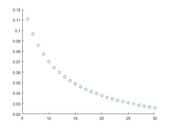
Figure 1. $c_{n}$ for $6\leq n\leq 30$

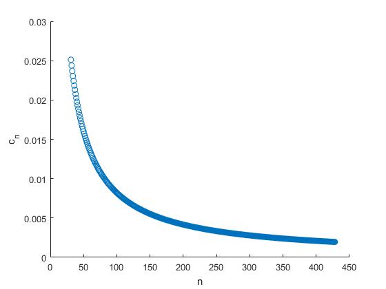
Figure 2. $c_{n}$ for $30\leq n\leq 428$

∎

Then we give the proof of Theorem 1.1 when $n$ is small.

Proof of Theorem 1.1 for $n<10000$.

We follow the argument in Section 4. We only prove for $n\geq 65$ (For the case when $5\leq n\leq 61$, we can use similar methods to run the induction procedure).

Applying Proposition 4.1 and plugging it into (4), we have

$$0\leq \frac{256}{35}(7-\frac{1}{\alpha})(\frac{27}{7\alpha}-15-\lambda_{n+1})\frac{1}{\alpha}(1-\frac{7}{6}a)+\frac{128}{7}(\lambda_{n+1}-6+\frac{71}{7\alpha})\frac{1}{\alpha^{2}}(1-\frac{7}{6}a)^{2}$$

$$+ \frac{176}{63}\alpha(\lambda_{2}+4)(\lambda_{2}+6)b_{2}^{2}$$

$$+ \frac{32}{9\alpha^{2}}\sum_{k=2}^{\frac{n-3}{2}}(\lambda_{n+1}-\lambda_{k}+\frac{11}{7\alpha})(2k+5)(1-\frac{1-b}{d}\lambda_{k}a)^{2}a^{2}$$

$$+ \frac{32}{9\alpha^{2}}\sum_{k=\frac{n-1}{2}}^{n}(\lambda_{n+1}-\lambda_{k}+\frac{11}{7\alpha})(2k+5)(ba+(1-b)\frac{d}{4\lambda_{k}})^{2}.$$

$$\leq -\frac{512}{7}(\lambda_{n+1}+\frac{51}{7})(1-\frac{7}{6}a)+\frac{512}{7}(\lambda_{n+1}+\frac{100}{7})(1-\frac{7}{6}a)^{2}+\frac{22528}{63\alpha}a^{2}$$

$$+ \frac{128}{9}\sum_{k=2}^{\frac{n-3}{2}}(\lambda_{n+1}-\lambda_{k}+\frac{22}{7})(2k+5)[(1-\frac{1-b}{d}\lambda_{k}a)^{2}+\frac{1}{2}c_{k}\chi_{\{5\leq n\leq 61\}}]a^{2}$$

$$+ \frac{128}{9}\sum_{k=\frac{n-1}{2}}^{n}(\lambda_{n+1}-\lambda_{k}+\frac{22}{7})(2k+5)[(ba+(1-b)\frac{d}{4\lambda_{k}})^{2}+\frac{1}{2}c_{k}\chi_{\{5\leq n\leq 61\}}]a^{2}$$

$$= :\tilde{g}_{n}(a).$$ (E.1)

To obtain a contradiction, it suffices to show that $\tilde{g}_{n}(a)$ is negative for $\frac{16}{\lambda_{n+4}}<a\leq\frac{16}{\lambda_{n}}$, for any $n<10000$ with $n\equiv 1\text{ (mod }4)$. Note that $\tilde{g}_{n}(a)$ is a parabola of $a$ with positive constant term. It suffices to show $\tilde{g}_{n}(\frac{16}{\lambda_{n+4}})$ and $\tilde{g}_{n}(\frac{16}{\lambda_{n}})$ are negative. Using Matlab, we obtain the following scatter diagrams for the above two quantities and thus we are done.

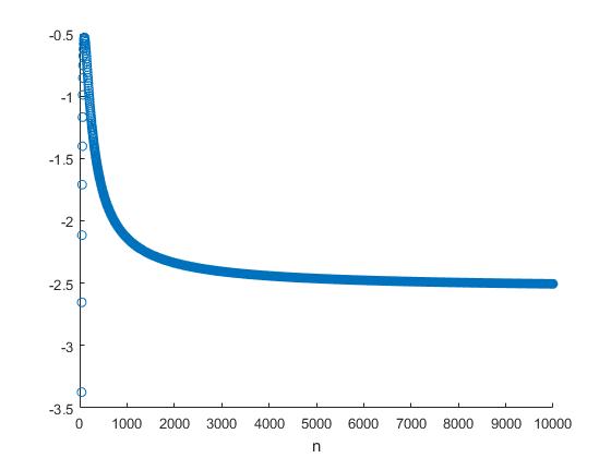
Figure 3. $\tilde{g}_{n}(\frac{16}{\lambda_{n+4}})$ from $n=41$ to $9997$

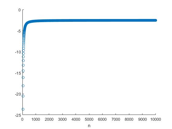
Figure 4. $\tilde{g}_{n}(\frac{16}{\lambda_{n}})$ from $n=41$ to $9997$

∎

References

- [1] I. Area, D. Dimitrov, E. Godoy, et al. Zeros of Gegenbauer and Hermite polynomials and connection coefficients, Mathematics of Computation. 73(248) (2004), 1937-1951.
- [2] F.W. Olver, D.W. Lozier, R.F. Boisvert, C.W. Clark, eds. NIST handbook of mathematical functions hardback and CD-ROM, Cambridge university press, 2010.
- [3] G. Szegö, Orthogonal Polynomials, 4th ed., Amer. Math. Soc. Coll. Publ., Vol. 23, Providence, RI, 1975
- [4] W. Beckner, Sharp Sobolev inequalities on the sphere and the Moser-Trudinger inequality, Ann. Math. 138 (1993), 213–242.
- [5] S.-Y.A. Chang and C. Gui, A sharp inequality on the exponentiation of functions on the sphere, Comm. Pure Appl. Math., to appear.
- [6] S.-Y.A. Chang and F.B. Hang, Improved Moser-Trudinger-Onofri Inequality under constraints, Comm. Pure Appl. Math. 75 (2022), 197–220.
- [7] S.-Y.A. Chang and P.C. Yang, Prescribing Gaussian curvature on , Acta Math. 159 (1987), 215–259.
- [8] S.-Y. A. Chang and P. C. Yang, Conformal deformation of metrics on S2. J. Differential Geom. 27 (1988), no. 2, 259–296.
- [9] S.-Y.A. Chang and P.C. Yang, Extremal metrics of zeta function determinants on 4-manifolds, Ann. Math. 142 (1995), 171–212.
- [10] S.-Y.A. Chang and P.C. Yang, On uniqueness of an nth order differential equation in conformal geometry, Math. Res. Lett. 4 (1997), 1–12.
- [11] Z. Djadli, E. Hebey and M. Ledoux, Paneitz-type operators and applications, Duke Math. J. 104(1) (2000), 129–169.
- [12] Z. Djadli and A. Malchiodi, Existence of conformal metrics with constant Q-curvature, Ann. Math. 168 (2008) 813–858.
- [13] J.Feldman, R. Froese, N. Ghoussoub and C.F. Gui, An improved Moser-Aubin-Onofri inequality for axially symmetric functions on S2. Calc. Var. Partial Differential Equations 6 (1998), no. 2, 95–104.
- [14] N. Ghoussoub and C. S. Lin, On the best constant in the Moser-Onofri-Aubin inequality. Comm. Math. Phys. 298 (2010), no. 3, 869–878.
- [15] C. Gui and A. Moradifam, The sphere covering inequality and its applications, Invent. Math. 214(3) (2018), 1169–1204.
- [16] C. Gui, Y. Hu and W. Xie, Improved Beckner’s inequality for axially symmetric functions on , arXiv :2109 .13390.
- [17] C. Gui, Y. Hu and W. Xie, Improved Beckner’s inequality for axially symmetric functions on , J. Funct. Analysis 282(2022), 109335.
- [18] C. Gui and J. Wei, On a sharp Moser-Aubin-Onofri inequality for functions on with symmetry, Pac. J. Math. 194(2) (2000) 349–358.
- [19] M. Gursky and A. Malchiodi, A strong maximum principle for the Paneitz operator and a non-local flow for the Q-curvature. J. Eur. Math. Soc. (JEMS) 17(9) (2015), 2137–2173.
- [20] T. Jin, Y. Li and J. Xiong, The Nirenberg problem and its generalizations: a unified approach. Math. Ann. 369 (2017), no. 1-2, 109–151.
- [21] Y.Y. Li and J.G. Xiong, Compactness of conformal metrics with constant Q-curvature, Adv. Math. 345 (2019), 116–160.
- [22] T. Li, J. Wei and Z. Ye, On sharp Beckner’s inequality for axially symmetric functions on , arXiv :2212.04099.
- [23] A. Malchiodi, Compactness of solutions to some geometric fourth-order equations, J. Reine Angew. Math. 594 (2006), 137–174.
- [24] M. Morimoto, Analytic Functionals on the Sphere, Translations of Mathematical Monographs, No 178. AMS, first edition, 1998.
- [25] G. Nemes and A. O. Daalhuis, Large-parameter asymptotic expansions for the Legendre and allied functions. SIAM J. Math. Anal. 52 (2020), no. 1, 437–470.
- [26] J. Wei and X. Xu, On conformal deformations of metrics on , J. Funct. Anal. 157 (1998), 292–325.