Forward Sensitivity Analysis and Mode Dependent Control for Closure Modeling of Galerkin Systems

Abstract

Model reduction by projection-based approaches is often associated with losing some of the important features that contribute towards the dynamics of the retained scales. As a result, a mismatch occurs between the predicted trajectories of the original system and the truncated one. We put forth a framework to apply a continuous time control signal in the latent space of the reduced order model (ROM) to account for the effect of truncation. We set the control input using parameterized models by following energy transfer principles. Our methodology relies on observing the system behavior in the physical space and using the projection operator to restrict the feedback signal into the latent space. Then, we leverage the forward sensitivity method (FSM) to derive relationships between the feedback and the desired mode-dependent control. We test the performance of the proposed approach using two test cases, corresponding to viscous Burgers and vortex merger problems at high Reynolds number. Results show that the ROM trajectory with the applied FSM control closely matches its target values in both the data-dense and data-sparse regimes.

1 Introduction

Engineers always tend to increase gains and reduce costs. For example, the airfoil design of an airplane wing is optimized to increase lift, reduce drag, and enhance stability. The design optimization process involves multiple forward runs to simulate the system’s response to different inputs, parameters, and operating conditions. This multi-query nature is often labeled as outer-loop applications while the individual forward simulations are known as inner-loop computations. For high dimensional systems (e.g., fluid flows), the wall-clock time for such computations becomes incompatible with desired turnaround times for design cycles as well as realtime control. This computational burden presents a roadblock to the routine use of simulation tools by industry. Therefore, lightweight surrogates are often sought to approximate the effective dynamics and reduce the computational costs of inner-loop computations without compromising the integrity of the computational pipeline [9, 6, 33, 8, 7, 54, 55, 72, 27, 59, 32, 48, 29].

With the advent of data-driven tools and open-source software libraries, machine learning (ML) algorithms have been exploited to build computationally light emulators solely from data. The complex input-output relationships are learnt from precollected recordings of the system’s dynamics during a compute-intensive process known as training. More recently, there has been an increasing interest in embedding existing knowledge to build hybrid physics informed ML frameworks [63, 31, 17, 73], possibly by considering feature enhancement [40], using prediction from simplified models as the bias [53, 51, 52], adopting transfer learning mechanisms [19, 23, 15], designing composite networks [41], implementing physics-informed neural networks [57, 30] and residual forcing [21], imposing conservation laws of physical quantities or analytical constraints into neural network [42, 11, 24], and embedding tensorial invariance and equivariance properties [38, 75, 46, 70].

Alternatively, projection-based reduced order models (PROMs) can be viewed as a physics-constrained ML methodology to emulate the system’s dynamics. In particular, an effective low rank subspace is identified by means of modal analysis techniques that tailor a set of basis functions or modes representative of the dominant recurrent structures. The underlying physical constraints are imposed by performing a Galerkin projection of the governing equations onto the respective basis functions. To ensure computational efficiency, only a few basis functions are retained to build the Galerkin reduced order model (GROM). The combination of modal decomposition and projection techniques have been widely applied to build lightweight computational models in flow control systems [45, 13, 49]. Nonetheless, the number of required modes to sufficiently describe systems of interest can be quite large. This is especially true for systems with strong nonlinearity or extreme variations in the parameter space. For such, the GROM fails to accurately represent the system’s trajectory. Moreover, GROM can yield long-term instabilities even if the original system is stable [1]. Therefore, correcting the GROM dynamics by introducing closure terms, stabilization schemes, or regularizers is a critical step to adopt them in a reliable framework.

The closure problem has been studied extensively in the fluid dynamics and flow control community. Structural and/or functional relationships are often postulated, then physical and mathematical arguments are imposed to define the required parameterization. Alternatively, we address the closure modeling problem by viewing its effect as a control input applied in the latent space (i.e., latent control or latent action) to counteract the induced instabilities and inaccuracies from the GROM truncation. In particular, we employ a continuous time control signal to correct and stabilize the GROM trajectory by deriving low-rank closure models using principles from the Kolmogorov energy cascade of turbulence and energy conservation. We utilize the forecast error, measured as the discrepancy between GROM predictions and collected sensor data, as the feedback and develop a variational approach to update the control input. In addition, we leverage the forward sensitivity method (FSM) to derive first-order estimates of the relationships between the feedback and the desired control parameters [35].

When dealing with deterministic models, whether they are continuous or discrete, the FSM approach can be employed to effectively rectify the forecast errors that arise from inaccuracies in the initial conditions, boundary conditions, and model parameters (collectively called control) [36]. Specifically, the FSM framework possesses a significant benefit, which is its independence from a backward adjoint formulation. Instead, it transforms a dynamic data assimilation problem into a static, deterministic inverse problem, thereby constituting the primary tenet of this approach. The FSM technique employs a linear Taylor series approximation to derive sensitivity dynamics for control parameters, subsequently facilitating the translation of recurrence matrix equations for forward sense. While the computation of these recurrence relations may be computationally intensive for high dimensional state problems, the FSM method holds considerable appeal for models based on latent space projection.

Our approach addresses the challenge of closure problems in under-resolved regimes by using a novel strategy to optimize control input parameters at the ROM level, which allows for a more accurate description of complex physical phenomena using a small number of modes. We highlight that one key aspect of the proposed framework is its flexibility in dealing with state variables and observables that live in distinct spaces. For example, the original system has a high dimensional state variable that lives in the physical space. In contrast, the reduced order system has a latent state variable defined in a low rank subspace. Finally, the observable output can be a different measurable quantity related to either space. This is conceptually related to the reduced order observers [18] and functional observers [34, 60, 44] developed in the control community. We demonstrate the proposed framework using the semi-discretized high dimensional flow problems corresponding to the Bateman–Burgers system and vortex merger at a large Reynolds number for the sensor data-rich and data-sparse regimes.

This paper is organized as follows. In Section 2, we introduce the key elements of building GROM for high dimensional dynamical systems using a combination of proper orthogonal decomposition (Section 2.1) and Galerkin projection (Section 2.2). The closure problem is formally defined in Section 3 and the proposed FSM-based control approach is presented in Section 4. Numerical experiments are provided in Section 5 with the corresponding discussions. Finally, Section 6 draws the main conclusions of the study and offers outlook for future work.

2 Galerkin Reduced Order Models

We consider an autonomous dynamical system defined as follows:

$${\color[rgb]{0,0,0}\dot{\boldsymbol{u}}=\mathcal{F}(\boldsymbol{u}),}$$ (1)

where $\boldsymbol{u}\in\mathbb{R}^{N}$ is the state vector (e.g., the value of the velocity field at discrete grid points) and $\mathcal{F}:\mathbb{R}^{N}\times\to\mathbb{R}^{N}$ represents the system’s dynamics (e.g., the spatial discretization of the Navier-Stokes equations). We note that Eq. 1 is often called the full order model (FOM) or high dimensional model (HDM) in ROM studies. Due to the computational complexity of solving Eq. 1 for large scale systems with millions of degrees of freedom (DOFs), FOMs are not feasible for multi-query applications (e.g., inverse problem and model predictive control). A possible mitigation strategy is to replace the state vector $\boldsymbol{u}$ with a lower rank approximation, where the solution is approximated using a few basis functions that capture the main characteristics of the system.

2.1 Proper Orthogonal Decomposition

Proper orthogonal decomposition (POD) is one of the modal decomposition techniques that has been used successfully over last few decades to define optimal low rank bases for the quantities of interest [66, 5, 10, 26, 16, 37, 71, 72]. The POD procedure begins with a set of pre-collected realizations of the system’s behavior (known as flow snapshots) at different times as follows:

$$\mathcal{U}:=\{\boldsymbol{u}^{(1)},\boldsymbol{u}^{(2)},\dots,\boldsymbol{u}^{(K)}\},$$ (2)

where $\boldsymbol{u}^{(i)}$ denotes the $i^{\text{th}}$ snapshot reshaped into a column vector. A Reynolds decomposition of the flow field $\boldsymbol{u}$ can be written as:

$$\boldsymbol{u}=\bar{\boldsymbol{u}}+\boldsymbol{u}^{\prime},$$ (3)

where $\bar{\boldsymbol{u}}$ is a reference field usually defined by the ensemble mean as follows:

$$\bar{\boldsymbol{u}}=\dfrac{1}{K}\sum_{i=1}^{K}\boldsymbol{u}^{(i)},$$ (4)

and thus $\boldsymbol{u}^{\prime}$ represents the fluctuating component of the field. POD (using the method of snapshots) seeks a low rank basis functions for the span of $\mathcal{U}^{\prime}:=\{\boldsymbol{u}^{\prime(1)},\boldsymbol{u}^{\prime(2)},\dots,\boldsymbol{u}^{\prime(K)}\}$ by defining a correlation matrix $\mathbf{C}\in\mathbb{R}^{K\times K}$ as follows:

$$[\mathbf{C}]_{ij}=(\boldsymbol{u}^{\prime(i)},\boldsymbol{u}^{\prime(j)}),$$ (5)

where $(\cdot,\cdot)$ denotes the appropriate inner product. An eigenvalue decomposition of $\mathbf{C}$ yields a set of eigenvectors $\mathbf{V}=[\mathbf{v}_{1},\mathbf{v}_{2},\dots\mathbf{v}_{K}]$ and the corresponding eigenvalues $\boldsymbol{\Lambda}=\text{diag}[\lambda_{1},\lambda_{2},\dots\lambda_{K}]$ as:

$$\mathbf{C}\mathbf{V}=\mathbf{V}\boldsymbol{\Lambda}.$$ (6)

For optimal basis selection, the eigenvalues are stored in descending order of magnitude (i.e., $\lambda_{1}\geq\lambda_{2}\geq\dots\geq\lambda_{K}\geq 0$). The POD basis functions $\boldsymbol{\Phi}=\{\boldsymbol{\phi}_{1},\boldsymbol{\phi}_{2},\dots\boldsymbol{\phi}_{K}\}$ can be recovered as follows:

$${\color[rgb]{0,0,0}\boldsymbol{\phi}_{i}=\dfrac{1}{\sqrt{\lambda_{i}}}\sum_{j=1}^{K}\mathbf{v}_{i,j}\boldsymbol{u}^{\prime(j)},}$$ (7)

where $\mathbf{v}_{i,j}$ is the $j^{\text{th}}$ component of the $i^{\text{th}}$ eigenvector. Finally, the $n^{\text{th}}$ rank POD approximation of $\boldsymbol{u}$ is obtained by considering only the first $n$ basis functions as follows:

$$\boldsymbol{u}\approx\bar{\boldsymbol{u}}+\sum_{i=1}^{n}a_{i}\boldsymbol{\phi}_{i}.$$ (8)

2.2 Galerkin Projection

In Eq. 8, the mean field $\bar{\boldsymbol{u}}$ and the basis functions $\boldsymbol{\Phi}$ are computed from the collected snapshots during an offline stage. In order to estimate $\boldsymbol{u}$ at arbitrary times and/or parameters, a model that describes the variation of the coefficients $\boldsymbol{a}=[a_{1},a_{2},\dots,a_{n}]^{T}$ is required. The Galerkin ROM (GROM) of the dynamical system governed by Eq. 1 is obtained by replacing $\boldsymbol{u}$ by its $n^{\text{th}}$ rank POD approximation from Eq. 8, followed by an inner product with arbitrary POD modes to yield the following system of ordinary differential equations:

$$\dot{a}_{k}=\bigg{(}\mathcal{F}(\bar{\boldsymbol{u}}+\sum_{i=1}^{n}a_{i}\boldsymbol{\phi}_{i}),\boldsymbol{\phi}_{k}\bigg{)},\quad\text{for }k=1,2,\dots,n.$$ (9)

We note that the simplification in the left hand-side of Eq. 9 takes advantage of the orthornomality of the POD basis function (i.e., $(\boldsymbol{\phi}_{i},\boldsymbol{\phi}_{j})=\delta_{ij}$ where $\delta_{ij}$ is the Kronecker delta). Without loss of generality, we consider the following incompressible Navier-Stokes equation (NSE) for demonstration purposes:

$$\dfrac{\partial\boldsymbol{u}}{\partial t}+(\boldsymbol{u}\cdot\nabla)\boldsymbol{u} =-\nabla p+\nu\Delta\boldsymbol{u},$$ (10)

$$\nabla\cdot\boldsymbol{u} =0,$$

where $\boldsymbol{u}$ is the velocity vector field, $p$ the pressure field, and $\nu$ is the kinematic viscosity. This form of the NSE captures the main characteristics of a large class of flow problems with quadratic nonlinearity and second order dissipation. In our results section, we showcase the applicability of the presented approach in the 1D Burgers problem and the 2D vortex-merger flow problem governed by the vortex transport equations. Applying the Galerkin method to Eq. 10, the resulting GROM reads as follows:

$$\dot{\boldsymbol{a}}=\boldsymbol{b}+\boldsymbol{L}\boldsymbol{a}+\boldsymbol{a}^{T}\boldsymbol{N}\boldsymbol{a},$$ (11)

where $\boldsymbol{b}\in\mathbb{R}^{n}$, $\boldsymbol{L}\in\mathbb{R}^{n\times n}$, and $\boldsymbol{N}\in\mathbb{R}^{n\times n\times n}$ respectively represent the constant, linear, and nonlinear terms that result from the inner product between the FOM operators and the POD basis functions.

3 The Closure Problem

Due to the modal truncation (i.e., using $n\ll K$ in Eq. 8), the effects of the truncated scales onto the resolved scales are not captured by Eq. 9. Therefore, the resulting GROM fails to accurately represent the dynamics of the ROM variables $\boldsymbol{a}$. Previous studies have shown that GROM yields inaccurate and sometimes unstable behavior even if the actual system is stable [25]. Therefore, efforts have been focused onto developing techniques to correct the GROM trajectory, including works to correct and/or stabilize the GROM using closure and/or regularization schemes [67]. As introduced in Section 1, we view the process of adjusting the GROM trajectory as a control task with a computational actuator in the latent space of the reduced order model.

To this end, we modify Eq. 11 by adding a control input $\boldsymbol{c}(t)=[c_{1},c_{2},\dots,c_{n}]^{T}$ as follows:

$$\dot{\boldsymbol{a}}=\boldsymbol{b}+\boldsymbol{L}\boldsymbol{a}+\boldsymbol{a}^{T}\boldsymbol{N}\boldsymbol{a}+\boldsymbol{c}(t).$$ (12)

The goal of the control $\boldsymbol{c}$ is to steer the GROM predictions toward the target trajectory defined as follows:

$$\widehat{a}_{k}(t)=\bigg{(}\boldsymbol{u}(t)-\bar{\boldsymbol{u}},\boldsymbol{\phi}_{k}\bigg{)},$$ (13)

where the superscript $\widehat{(\cdot)}$ denotes the target values. It can be verified that the trajectory given in Eq. 13 with the POD basis functions $\boldsymbol{\phi}_{k}$ yields the minimum approximation error among all possible reconstructions of rank-$n$ (or less) [26]. The control input that would result in values of $\boldsymbol{a}$ that are exactly equal to their optimal values in Eq. 13 can be defined as follows:

$$c_{k}(t)=\bigg{(}\mathcal{F}(\boldsymbol{u}),\boldsymbol{\phi}_{k}\bigg{)}-\bigg{(}\mathcal{F}(\bar{\boldsymbol{u}}+\sum_{i=1}^{n}a_{i}\boldsymbol{\phi}_{i}),\boldsymbol{\phi}_{k}\bigg{)}.$$ (14)

Equation 14 essentially leads to the following:

$$\dot{a}_{k}=\bigg{(}\mathcal{F}(\boldsymbol{u}),\boldsymbol{\phi}_{k}\bigg{)},$$ (15)

which is an exact equation (i.e., no truncation) for the dynamics of $\boldsymbol{a}$. However, we highlight that Eq. 14 is not useful in practice as it requires solving the FOM to compute $\boldsymbol{u}$ at each time step. Therefore, alternative approximate models are sought to estimate $\boldsymbol{c}$ as a function of the available information in the ROM subspace (i.e., $\{a_{k},\phi_{k}\}_{k=1}^{n}$). To account for the effect of ROM truncation onto the dynamics of ROM scales themselves is often referred to as the closure problem.

The development of closure models for ROMs has been largely influenced by turbulence modeling and especially large eddy simulation (LES) studies. For example, by analogy between POD modes and Fourier modes, it is often postulated that the high-index modes (i.e., $\{\phi_{k}\}_{k>n}$) are responsible for dissipating the energy. In turn, by truncating these modes, energy accumulates in the systems causing instabilities. In this regard, the addition of artificial dissipation through eddy viscosity has shown substantial success in improving ROM accuracy [12, 3, 74, 61]. Nonetheless, the determination of the eddy viscosity term has been a major challenge. Several studies relied on brute-force search to select optimal values while other works were inspired by state-of-the-art LES models [1], such as the Smagorinksy model [3, 62] or its dynamic counterparts [74, 56]. Noack et al. [45] utilized a finite-time thermodynamics approach to quantify a nonlinear eddy viscosity by matching the modal energy transfer effect. A notably distinct closure model was proposed in [14] by adding a linear damping term to the ROM equation. This model is predefined using the collected ensemble of snapshots following an energy conservation analysis.

The present study draws concepts from the Kolmogorov energy cascade and energy conservation principles to define the effect of the modal truncation on ROM dynamics. In order to derive the form of the closure model, we add a combination of linear friction and diffusion terms to Eq. 10 as follows:

$$\dfrac{\partial\boldsymbol{u}}{\partial t}+(\boldsymbol{u}\cdot\nabla)\boldsymbol{u}=-\nabla p+\nu\Delta\boldsymbol{u}+\gamma\boldsymbol{u}+\beta\Delta\boldsymbol{u},$$ (16)

where $\gamma$ and $\beta$ are the friction and diffusion parameters, respectively. Projecting Eq. 16 onto the POD subspace leads to a model for $\boldsymbol{c}$ as follows:

$$\boldsymbol{c}(t) =\gamma\boldsymbol{e}+\gamma\boldsymbol{a}+\beta\boldsymbol{q}+\beta\boldsymbol{D}\boldsymbol{a}$$ (17)

$$\text{where: }\qquad[\boldsymbol{e}]_{k} =\big{(}\bar{\boldsymbol{u}},\boldsymbol{\phi}_{k}\big{)},\quad[\boldsymbol{q}]_{k}=\big{(}\Delta\bar{\boldsymbol{u}},\boldsymbol{\phi}_{k}\big{)},\quad[\boldsymbol{D}]_{k,i}=\big{(}\Delta\boldsymbol{\phi}_{i},\boldsymbol{\phi}_{k}\big{)}.\quad$$ (18)

Thus, we aim at correcting the GROM trajectory by estimating optimal values for $\gamma$ and $\beta$ and we refer to them as the control parameters or simply the control. However, we highlight that even if we hypothesize that the correction term can be approximated using Eq. 17, this approximation is by no means exact. Instead, we are interested in values of $\alpha$ and $\beta$ that would result in the least error (with respect to a set of reference data points). In addition, it should be noted here that inconsistency issues (between the full order model and reduced order model) might arise from the introduction of arbitrary closure models. We refer the interested readers to [47, 22, 68, 69]. In the present study, we set $\gamma=[\gamma_{1},\gamma_{2},\dots,\gamma_{n}]^{T}\in\mathbb{R}^{n}$ and $\beta=[\beta_{1},\beta_{2},\dots,\beta_{n}]^{T}\in\mathbb{R}^{n}$ to allow variability of the closure model with different modes. The use of mode-dependent correction has been shown to provide better closure models, e.g., by matching energy levels between FOM and ROM [58], incorporating spectral kernels [65, 61], or utilizing the variational multiscale framework [74, 28, 20].

4 Forward Sensitivity Method

We leverage the forward sensitivity method (FSM) [35, 36] to estimate the parameters $\gamma$ and $\beta$ from a combination of the underling dynamical model and collected observational data. To simplify our notation, we rewrite Eq. 12, with $\boldsymbol{c}(t)$ defined using Eq. 17, as follows:

$$\dot{\boldsymbol{a}}=\boldsymbol{f}(\boldsymbol{a},\boldsymbol{\theta}),$$ (19)

where

$$\boldsymbol{f}(\boldsymbol{a},\boldsymbol{\theta})=\boldsymbol{b}+\boldsymbol{L}\boldsymbol{a}+\boldsymbol{a}^{T}\boldsymbol{N}\boldsymbol{a}+\gamma\boldsymbol{e}+\gamma\boldsymbol{a}+\beta\boldsymbol{q}+\beta\boldsymbol{D}\boldsymbol{a}$$ (20)

and

$$\boldsymbol{\theta}=[\gamma_{1},\gamma_{2},\dots,\gamma_{n},\beta_{1},\beta_{2},\dots,\beta_{n}]^{T}\in\mathbb{R}^{2n}$$ (21)

denotes the control parameters. In what follows, we use a set of collected, possibly sparse and noisy, measurements to approximate how the predictions of Eq. 19 deviate from their target values. In addition, we describe how these predictions depend on the control parameter $\boldsymbol{\theta}$ in Section 4.2. Finally, we fuse these two pieces of information to derive a relationship between the model predictions, temporal measurements, and the corrected parameter values in Section 4.3.

4.1 Forecast Error and Feedback

We monitor the model behavior by collecting a set of measurements $\boldsymbol{z}\in\mathbb{R}^{m}$ as follows:

$$\boldsymbol{z}(t)=\boldsymbol{h}(\widehat{\boldsymbol{a}(t)})+\eta(t),$$ (22)

where $\boldsymbol{h}(\cdot):\mathbb{R}^{n}\to\mathbb{R}^{m}$ represents the observational operator, $\widehat{\boldsymbol{a}}$ is the true value of the model state $\boldsymbol{a}$, and $\eta$ is the sensor measurement noise. We note that the measurement $\boldsymbol{z}$ is a function of the ground truth and the observation operator can involve a sampling operation, an interpolation, or even a mapping between different spaces. Therefore, the dimensionality $m$ of the observation $\boldsymbol{z}$ is not necessarily equal to the dimensionality $n$ of the state $\boldsymbol{a}$.

For the measurement noise, we consider a white Gaussian perturbation (i.e., $\eta(t)\sim\mathcal{N}(\mathbf{0},\mathbf{R}(t))$, where $\mathbf{R}(t)$ denotes the measurement noise covariance matrix). In most cases, $\mathbf{R}(t)$ is a diagonal matrix implying that the measurement noise from different sensors are uncorrelated to each other. For simplicity, we assume that $\mathbf{R}(t)=\sigma^{2}\mathbf{I}_{m}$, where $\sigma$ is the standard deviation for the measurement noise and $\mathbf{I}_{m}$ is the $m\times m$ identity matrix. Due to deviations between the target trajectory (corresponding Eq. 13) and the GROM solution, the resulting forecast error can be written as follows:

$$\boldsymbol{\epsilon}(t)=\boldsymbol{z}(t)-\boldsymbol{h}(\boldsymbol{a}(t)).$$ (23)

The definition of the operator $\boldsymbol{h}(\cdot)$ is an important component of the whole setup. One option is to stick to the fact that measurements are often collected in the physical space and thus define the forecast error in this space. Considering the Burgers problem with a velocity field $\boldsymbol{u}\in\mathbb{R}^{N}$, we might be able to collect only data for $\boldsymbol{v}\in\mathbb{R}^{M}$ that is related to $\boldsymbol{u}$ as $\boldsymbol{v}=\mathcal{H}(\boldsymbol{u})$, where $\mathcal{H}(\boldsymbol{u})$ is an observation operator in the physical space of $\mathbf{u}$, compared to $\boldsymbol{h}(\boldsymbol{a})$ that is applied in the latent space of $\boldsymbol{a}$. Thus, by setting $\boldsymbol{z}=\boldsymbol{v}$ (i.e., $m=M$), we have $\boldsymbol{h}(\boldsymbol{a})=\mathcal{H}\big{(}\bar{\boldsymbol{u}}+\sum_{i=1}^{n}a_{i}\phi_{i}\big{)}$. Another computationally attractive option is to define the forecast error in a latent space defined as follows:

$$\boldsymbol{v}=\sum_{i=1}^{m}z_{i}\boldsymbol{\psi}_{i},$$ (24)

where $\{\boldsymbol{\psi}_{i}\}_{i=1}^{m}$ is some low rank basis for $\boldsymbol{v}$ [50]. Considering a POD basis $\boldsymbol{\psi}$, the components of $\boldsymbol{z}$ can be computed by projecting the field $\boldsymbol{v}$ on the respective basis functions as $z_{i}(t)=\big{(}\boldsymbol{v}(t),\boldsymbol{\psi}_{i}\big{)}$. Therefore, the observation operator $\boldsymbol{h}(\cdot)$ can be defined as follows:

$$[\boldsymbol{h}(\boldsymbol{a})]_{k}=\bigg{(}\mathcal{H}\big{(}\bar{\boldsymbol{u}}+\sum_{i=1}^{n}a_{i}\phi_{i}\big{)},\boldsymbol{\psi}_{k}\bigg{)}.$$ (25)

4.2 Sensitivity Dynamics

Since our objective is to relate the feedback $\boldsymbol{\epsilon}$ to the desired control parameters $\boldsymbol{\theta}$, we first need to define how these parameters affect the model predictions. Thus, we define the sensitivity of the model forecast $\boldsymbol{a}$ at any time $t$ with respect to the model’s parameters $\boldsymbol{\theta}$ using $\mathbf{V}\in\mathbb{R}^{n\times 2n}$ as follows,

$${\color[rgb]{0,0,0}[\mathbf{V}(t)]_{ij}=\bigg{[}\dfrac{\partial a_{i}(t)}{\partial\theta_{j}}\bigg{]}.}$$ (26)

By differentiating the dynamical model (i.e., Eq. 19) with respect to its parameters $\boldsymbol{\theta}$ and using the chain rule, it can be verified that $\mathbf{V}(t)$ evolves according to the following linear system:

$$\dot{\mathbf{V}}(t)=\mathbf{D}_{\boldsymbol{f}}(t)\mathbf{V}(t)+\mathbf{D}_{\boldsymbol{f}}^{\boldsymbol{\theta}}(t),$$ (27)

where $\mathbf{D}_{\boldsymbol{f}}$ and $\mathbf{D}_{\boldsymbol{f}}^{\boldsymbol{\theta}}$ symbolize the Jacobian of the model $\boldsymbol{f}$ with respect to the state $\boldsymbol{a}$ and parameters $\boldsymbol{\theta}$, respectively as follows:

$$\mathbf{D}_{\boldsymbol{f}} =\begin{bmatrix}\dfrac{\partial f_{1}}{\partial a_{1}}&&\dfrac{\partial f_{1}}{\partial a_{2}}&&\dots&&\dfrac{\partial f_{1}}{\partial a_{n}}\\ \\ \dfrac{\partial f_{2}}{\partial a_{1}}&&\dfrac{\partial f_{2}}{\partial a_{2}}&&\dots&&\dfrac{\partial f_{2}}{\partial a_{n}}\\ \\ \vdots&&\vdots&&\ddots&&\vdots\\ \\ \dfrac{\partial f_{n}}{\partial a_{1}}&&\dfrac{\partial f_{n}}{\partial a_{2}}&&\dots&&\dfrac{\partial f_{n}}{\partial a_{n}}\end{bmatrix}\in\mathbb{R}^{n\times n},$$ (28)

$$\mathbf{D}_{\boldsymbol{f}}^{\boldsymbol{\theta}} =\setcounter{MaxMatrixCols}{15}\begin{bmatrix}\dfrac{\partial f_{1}}{\partial\gamma_{1}}&&\dfrac{\partial f_{1}}{\partial\gamma_{2}}&&\dots&&\dfrac{\partial f_{1}}{\partial\gamma_{n}}&&\dfrac{\partial f_{1}}{\partial\beta_{1}}&&\dfrac{\partial f_{1}}{\partial\beta_{2}}&&\dots&&\dfrac{\partial f_{1}}{\partial\beta_{n}}\\ \\ \dfrac{\partial f_{2}}{\partial\gamma_{1}}&&\dfrac{\partial f_{2}}{\partial\gamma_{2}}&&\dots&&\dfrac{\partial f_{2}}{\partial\gamma_{n}}&&\dfrac{\partial f_{2}}{\partial\beta_{1}}&&\dfrac{\partial f_{2}}{\partial\beta_{2}}&&\dots&&\dfrac{\partial f_{2}}{\partial\beta_{n}}\\ \\ \vdots&&\vdots&&\ddots&&\vdots&&\vdots&&\vdots&&\ddots&&\vdots\\ \\ \dfrac{\partial f_{n}}{\partial\gamma_{1}}&&\dfrac{\partial f_{n}}{\partial\gamma_{2}}&&\dots&&\dfrac{\partial f_{n}}{\partial\gamma_{n}}&&\dfrac{\partial f_{n}}{\partial\beta_{1}}&&\dfrac{\partial f_{n}}{\partial\beta_{2}}&&\dots&&\dfrac{\partial f_{n}}{\partial\beta_{n}}\end{bmatrix}\in\mathbb{R}^{n\times 2n}$$

Since the initial conditions of the model sate (i.e., $\boldsymbol{a}(0)$) is independent of the model’s parameters, we can set $\mathbf{V}(0)=0$. Therefore, Eq. 27 can be solved along with Eq. 19 to compute the model’s predictions at any time as well as the sensitivity of such predictions to the model’s parameters.

4.3 Parameter Estimation

The deviations in the GROM trajectory and closure model parameterizations are denoted $\delta\boldsymbol{a}=\widehat{\boldsymbol{a}}-\boldsymbol{a}$ and $\delta\boldsymbol{\theta}=\widehat{\boldsymbol{\theta}}-\boldsymbol{\theta}$, respectively, where the superscript $\widehat{(\cdot)}$ corresponds to their target values. Thus, Eq. 26 can be used to relate $\delta\boldsymbol{a}$ to $\delta\boldsymbol{\theta}$ as:

$$\delta\boldsymbol{a}(t)=\mathbf{V}(t)\delta\boldsymbol{\theta}.$$ (29)

The first order Taylor expansion of $\boldsymbol{h}(\cdot)$ around $\boldsymbol{a}$ can be written as $\boldsymbol{h}(\boldsymbol{a}_{T})=\boldsymbol{h}(\boldsymbol{a})+\mathbf{D}_{\boldsymbol{h}}(\boldsymbol{a})\delta\boldsymbol{a}$, where $\mathbf{D}_{\boldsymbol{h}}$ is the Jacobian of the observation operator $\boldsymbol{h}$. Therefore, the forecast error $\boldsymbol{\epsilon}(t)$ in Eq. 23 can be rewritten as follows:

$$\boldsymbol{\epsilon}(t) =\boldsymbol{z}(t)-\boldsymbol{h}(\boldsymbol{a}(t))$$ (30)

$$=\boldsymbol{h}(\widehat{\boldsymbol{a}}(t))+\eta(t)-\boldsymbol{h}(\boldsymbol{a}(t))$$

$$=\cancel{\boldsymbol{h}(\boldsymbol{a}(t))}+{\color[rgb]{0,0,0}\mathbf{D}_{\boldsymbol{h}}(\boldsymbol{a}(t))\delta\boldsymbol{a}(t)}+\eta(t)-\cancel{\boldsymbol{h}(\boldsymbol{a}(t))}$$

$$={\color[rgb]{0,0,0}\mathbf{D}_{\boldsymbol{h}}(\boldsymbol{a}(t))\delta\boldsymbol{a}(t)+\eta(t)}.$$

Thus, the deterministic component of the forecast error $\boldsymbol{\epsilon}$ is linked to the correction $\delta\boldsymbol{\theta}$ through following relation:

$$\boldsymbol{\epsilon}(t)=\mathbf{D}_{\boldsymbol{h}}(\boldsymbol{a})\mathbf{V}(t)\delta\boldsymbol{\theta}.$$ (31)

Equation 31 is a linear system, in the standard form of $\mathbf{A}\mathbf{x}=\mathbf{b}$. It can be written for all time instances at which observational data are available. For example, assuming measurements are collected at $t_{1},t_{2},\dots,t_{T}$ we can build the following linear system:

$$\underbrace{\begin{bmatrix}\boldsymbol{z}(t_{1})-\boldsymbol{h}(\boldsymbol{a}(t_{1}))\\ \boldsymbol{z}(t_{2})-\boldsymbol{h}(\boldsymbol{a}(t_{2}))\\ \vdots\\ {\color[rgb]{0,0,0}\boldsymbol{z}(t_{T})}-\boldsymbol{h}(\boldsymbol{a}(t_{T}))\end{bmatrix}}_{\boldsymbol{\xi}\in\mathbb{R}^{Tm\times 1}}=\underbrace{\begin{bmatrix}\mathbf{D}_{\boldsymbol{h}}(\boldsymbol{a})\mathbf{V}(t_{1})\\ \mathbf{D}_{\boldsymbol{h}}(\boldsymbol{a})\mathbf{V}(t_{2})\\ \vdots\\ \mathbf{D}_{\boldsymbol{h}}(\boldsymbol{a})\mathbf{V}(t_{T})\end{bmatrix}}_{\mathbf{H}\in\mathbb{R}^{Tm\times 2n}}\begin{bmatrix}\delta\boldsymbol{\theta}\end{bmatrix}$$ (32)

and linear system solvers can be utilized to compute optimal values for the parameters $\boldsymbol{\theta}$. Furthermore, to account for the fact that the measurements, and hence the forecast errors, are subject to uncertainty, we use a weighted least-squares approach with $\mathbf{R}^{-1}$ being the weighting matrix, where $\mathbf{R}$ is a block-diagonal matrix constructed as follows,

$$\mathbf{R}=\begin{bmatrix}\mathbf{R}(t_{1})&&&\\ &\mathbf{R}(t_{2})&&\\ &&\ddots&\\ &&&{\color[rgb]{0,0,0}\mathbf{R}(t_{T})}\end{bmatrix}\in\mathbb{R}^{Tm\times Tm}.$$ (33)

In particular, the solution of the resulting linear system can be written as follows:

$$\delta\boldsymbol{\theta}\in\mathbb{R}^{2n\times 1}=\begin{cases}\left(\mathbf{H}^{T}\mathbf{R}^{-1}\mathbf{H}\right)^{-1}\mathbf{H}^{T}\mathbf{R}^{-1}\boldsymbol{\xi},&\quad\text{over-determined: }Tm>2n,\\ \mathbf{R}^{-1}\mathbf{H}^{T}\left(\mathbf{H}\mathbf{R}^{-1}\mathbf{H}^{T}\right)^{-1}\boldsymbol{\xi},&\quad\text{under-determined: }Tm<2n.\end{cases}$$ (34)

The solution of Eq. 34 is repeated until convergence is obtained (i.e., no more updates to $\boldsymbol{\theta}$ is needed, as shown in the psoudecode given by Algorithm 1).

Algorithm 1 Pseudocode of the forward sensitivity method for parameter estimation.

1:Start with the initial value of control $\boldsymbol{\theta}$ and compute the model trajectory $\boldsymbol{a}(t)$

2:Compute sensitivity dynamics $\mathbf{V}(t)$

3:Assemble $\mathbf{H}$

4:Solve $\mathbf{H}\delta\boldsymbol{\theta}=\boldsymbol{\xi}$ as a weighted linear least squares using the weight $\mathbf{R}^{-1}$

5:Set $\boldsymbol{\theta}\leftarrow\boldsymbol{\theta}+\delta\boldsymbol{\theta}$

Figure 1 depicts the process of identifying a lower order model for a high dimensional system and the use of the forward sensitivity framework to parameterize closure models that corrects the truncated GROM predictions. It is worth noting that once the measurement data are incorporated to estimate the parameter $\boldsymbol{\theta}$, the model Eq. 19 can be used to make predictions at any time (i.e., not restricted to the instants when measurement data are available).

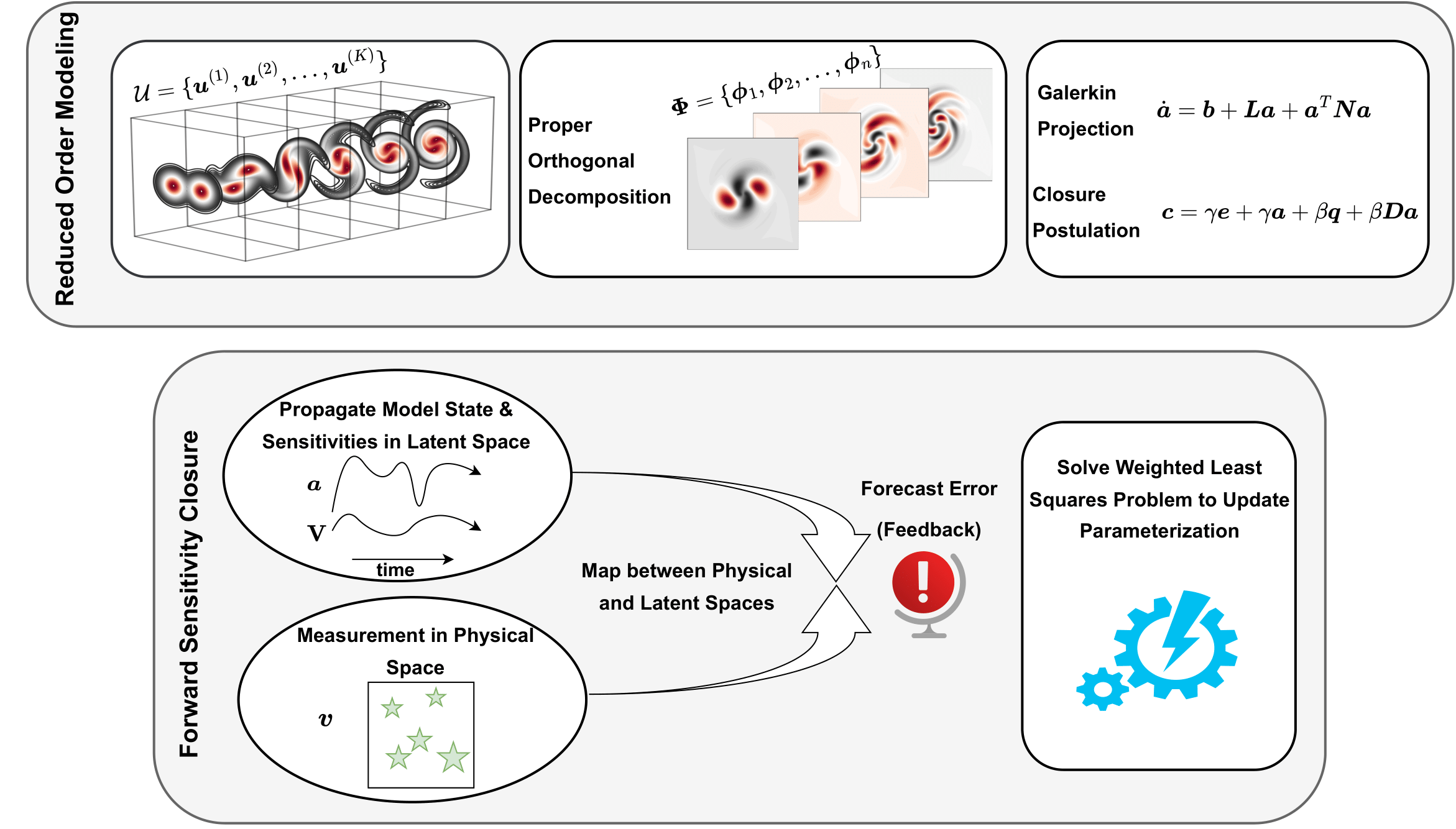
Figure 1: A schematic illustration of the algorithmic steps for deriving a Galerkin reduced order model (top) and closure modeling in the form of a latent control input using a forward sensitivity analysis (bottom).

5 Results & Discussion

We demonstrate the FSM closure framework using two canonical test problems with different levels of complexity. The first case deals with a one dimensional nonlinear advection diffusion system governed by the viscous Burgers equation, which is considered the 1D version of the NSE (see Eq. 10). In the second demonstration, we consider the two dimensional vortex merger problem governed by the vorticity transport equation (i.e., the curl of the two dimensional NSE). We study the cases of full field measurement and the more practical scenario when only very sparse sensor data are available.

5.1 Viscous Burgers Problem

The 1D viscous Burgers problem can be written as:

$$\dfrac{\partial u}{\partial t}+u\dfrac{\partial u}{\partial x}=\nu\dfrac{\partial^{2}u}{\partial x^{2}}.$$ (35)

We perform our numerical experiments at a Reynolds number $\text{Re}=10,000$, which is equivalent to setting $\nu=10^{-4}$ in Eq. 35. For FOM solution, we utilize a family of compact finite difference schemes for spatial discretization and the third order total variation diminishing Runge-Kutta (TVD-RK3) scheme for temporal integration [61]. We assume an initial condition of a unit step function as follows:

$$\boldsymbol{u}(x,0)=\begin{cases}1,\quad\text{if}\quad x\in[0,0.5],\\ 0,\quad\text{if}\quad x\in(0.5,1].\end{cases}$$ (36)

We divide the spatial domain into $4096$ equally spaced intervals and utilize a time step of $\Delta t_{FOM}=10^{-4}$ for the FOM solution. We store velocity field snapshots every $100$ time steps to perform the POD analysis. For GROM, we retain $n=6$ modes to approximate the velocity field. An eigenvalue analysis reveals that $6$ modes capture about $92\%$ of the total system turbulent kinetic energy defined as $\frac{1}{2}\langle u_{i}u_{i}\rangle$, where $\langle\cdot\rangle$ denotes an averaging operation. In particular, we use the relative information content (RIC) metric, as shown in Fig. 2 and defined as follows:

$$\text{RIC}(n)=\dfrac{\sum_{i=1}^{n}\lambda_{i}}{\sum_{i=1}^{m}\lambda_{i}}\times 100.$$ (37)

The inner product between Eq. 35 and the POD basis functions leads to the GROM in Eq. 11, where the corresponding coefficients can be defined as follows:

_k $$=\bigg{(}\nu\dfrac{\partial^{2}\bar{u}}{\partial x^{2}}-\bar{u}\dfrac{\partial\bar{u}}{\partial x},\boldsymbol{\phi}_{k}\bigg{)},$$ (38)

$$[\boldsymbol{L}]_{k,i} =\bigg{(}\nu\dfrac{\partial^{2}\boldsymbol{\phi}_{i}}{\partial x^{2}}-\bar{u}\dfrac{\partial\boldsymbol{\phi}_{i}}{\partial x}-\boldsymbol{\phi}_{i}\dfrac{\partial\bar{u}}{\partial x},\boldsymbol{\phi}_{k}\bigg{)},$$

$$[\boldsymbol{N}]_{k,i,j} =\bigg{(}-\boldsymbol{\phi}_{i}\dfrac{\partial\boldsymbol{\phi}_{j}}{\partial x},\boldsymbol{\phi}_{k}\bigg{)}.$$

The time integration of the GROM model is carried out using a time step of $\Delta t_{ROM}=0.01$, which is $100$ times larger than $\Delta t_{FOM}$. Although $6$ POD modes represent more than $92\%$ of the total system energy, the GROM fails to correctly capture their temporal dynamics as we shall see in the following discussions. This exemplifies the need for a mechanism to correct the GROM predictions. The modified Burgers equation to admit the closure model can be written as follows:

$$\dfrac{\partial u}{\partial t}+u\dfrac{\partial u}{\partial x}=\nu\dfrac{\partial^{2}u}{\partial x^{2}}+\gamma u+\beta\dfrac{\partial^{2}u}{\partial x^{2}},$$ (39)

and the resulting closure model terms in Eq. 17 are

$$[\boldsymbol{e}]_{k}=\big{(}\bar{u},\boldsymbol{\phi}_{k}\big{)},\qquad[\boldsymbol{q}]_{k}=\bigg{(}\dfrac{\partial^{2}\bar{u}}{\partial x^{2}},\boldsymbol{\phi}_{k}\bigg{)},\qquad[\boldsymbol{D}]_{k,i}=\bigg{(}\dfrac{\partial^{2}\boldsymbol{\phi}_{i}}{\partial x^{2}},\boldsymbol{\phi}_{k}\bigg{)}.$$ (40)

In Section 5.1.1, we use full field measurement data to parameterize such model and in Section 5.1.2 we deal with the sparse data regime.

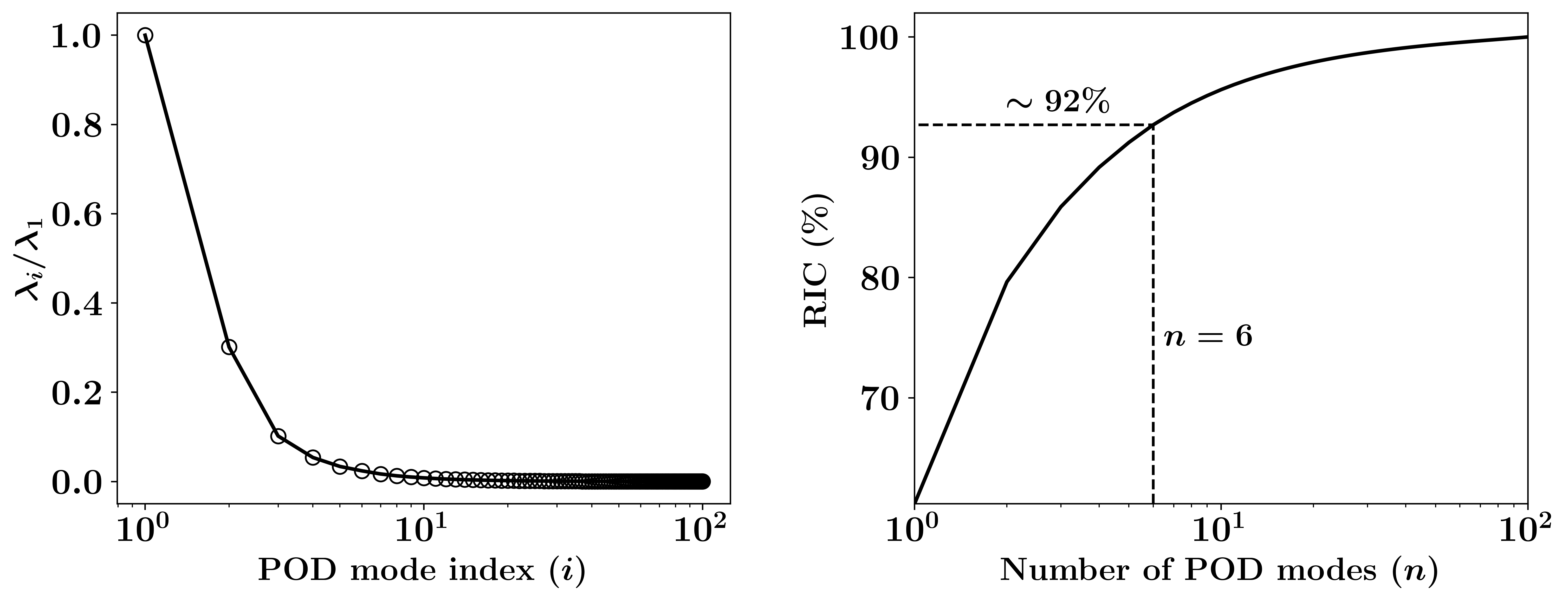
Figure 2: The decay of eigenvalues (left) and behavior of relative information content (right) for the 1D Burgers problem at $\text{Re}=10^{4}$.

5.1.1 Full field observations

We assume that the sensor signal is contaminated by a white Gaussian noise with zero mean and standard deviation of $0.1$, which represents $10\%$ of the peak velocity. In other words, we define $\boldsymbol{v}=\boldsymbol{u}+\eta$ where $\eta\sim\mathcal{N}(0,0.01\mathbf{I})$ and thus $[\boldsymbol{z}(t)]_{i}=(\boldsymbol{v}(t)-\bar{\boldsymbol{u}},\boldsymbol{\phi}_{i})$ (see Section 4.1). We collect measurement after every 10 time integrations of the GROM (i.e., $\Delta t_{Obs}=0.1$).

We refer to the solution with the target trajectory (given by Eq. 13) as prediction with “True Closure” notion. On the other hand, the solution of the uncontrolled GROM (i.e., Eq. 11) is denoted as the “No Closure” solution. Finally, the solution of the controlled GROM (i.e., Eq. 12) with FSM used to parameterize the presumed closure model in Eq. 17 is labeled as “FSM Closure”.

Figure 3 depicts the predicted dynamics in the latent ROM space using the considered different approaches. We observe that GROM leads to inaccuracies and significantly amplifies the magnitude of predicted coefficients, especially for the last mode. This behavior is likely to cause long term instabilities in the solution even if the actual system is stable. On the other hand, the FSM effectively controls the GROM trajectory and keeps it closer to the target trajectory. We emphasize that we implement a mode-dependent control to respect the distinct characteristics of the resolved modes defining recurrent flow structures.

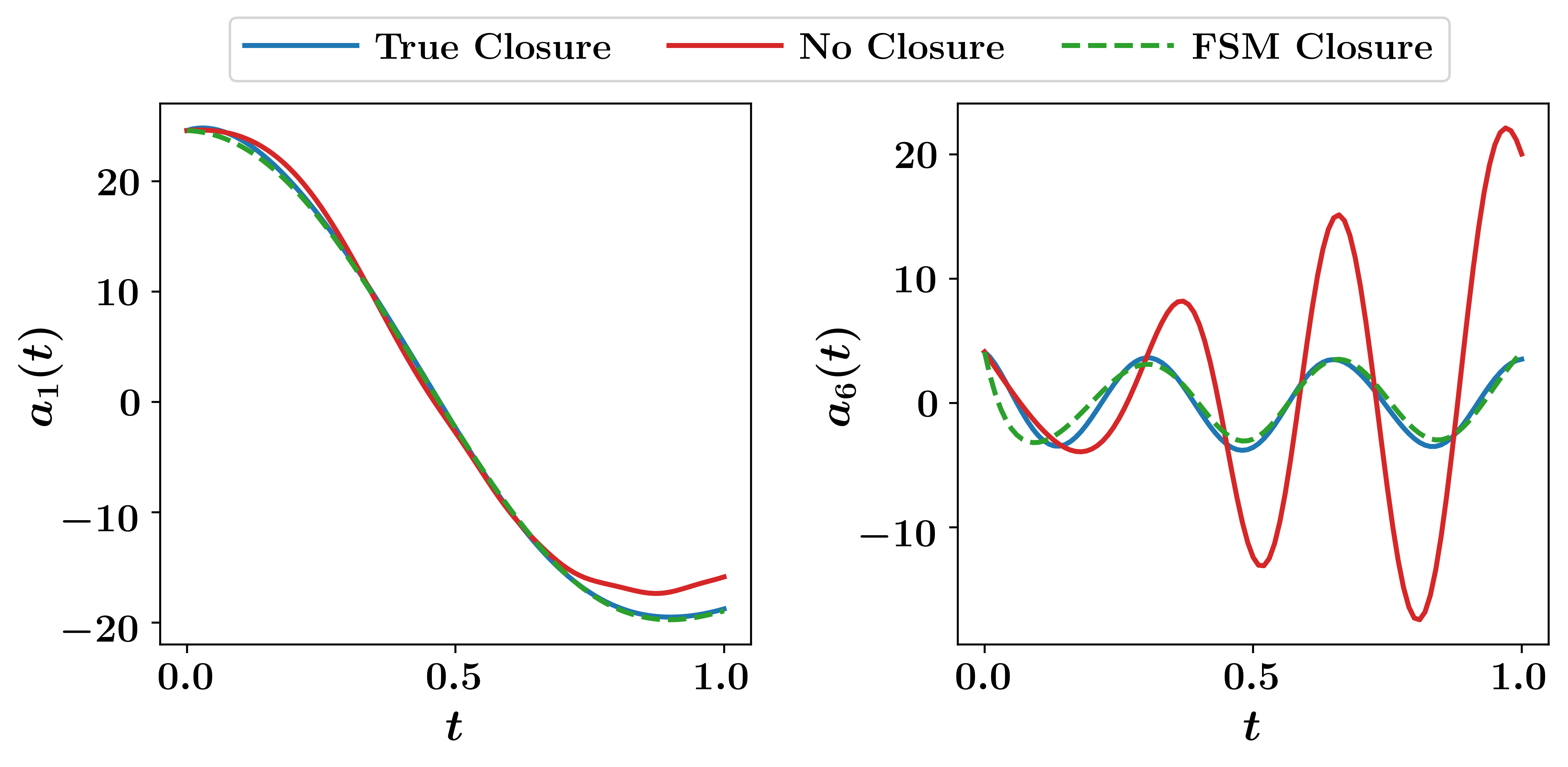
Figure 3: Dynamics of the first and last modal coefficients with full field measurement for the FSM Closure.

In Fig. 4, we evaluate the performance in the physical space by computing the reconstructed flow field using Eq. 8 compared to the FOM fields. In addition, the relative error for the predicted POD coefficients as well as the reconstructed velocity fields as a function of time is shown in Fig. 5. We see that results from FSM Closure are close to the True Closure which represents the minimum reconstruction error that could be obtained using $6$ modes. On the other hand, vanilla-type GROM without closure yields inaccurate and even non-physical solution in the spatio-temporal space.

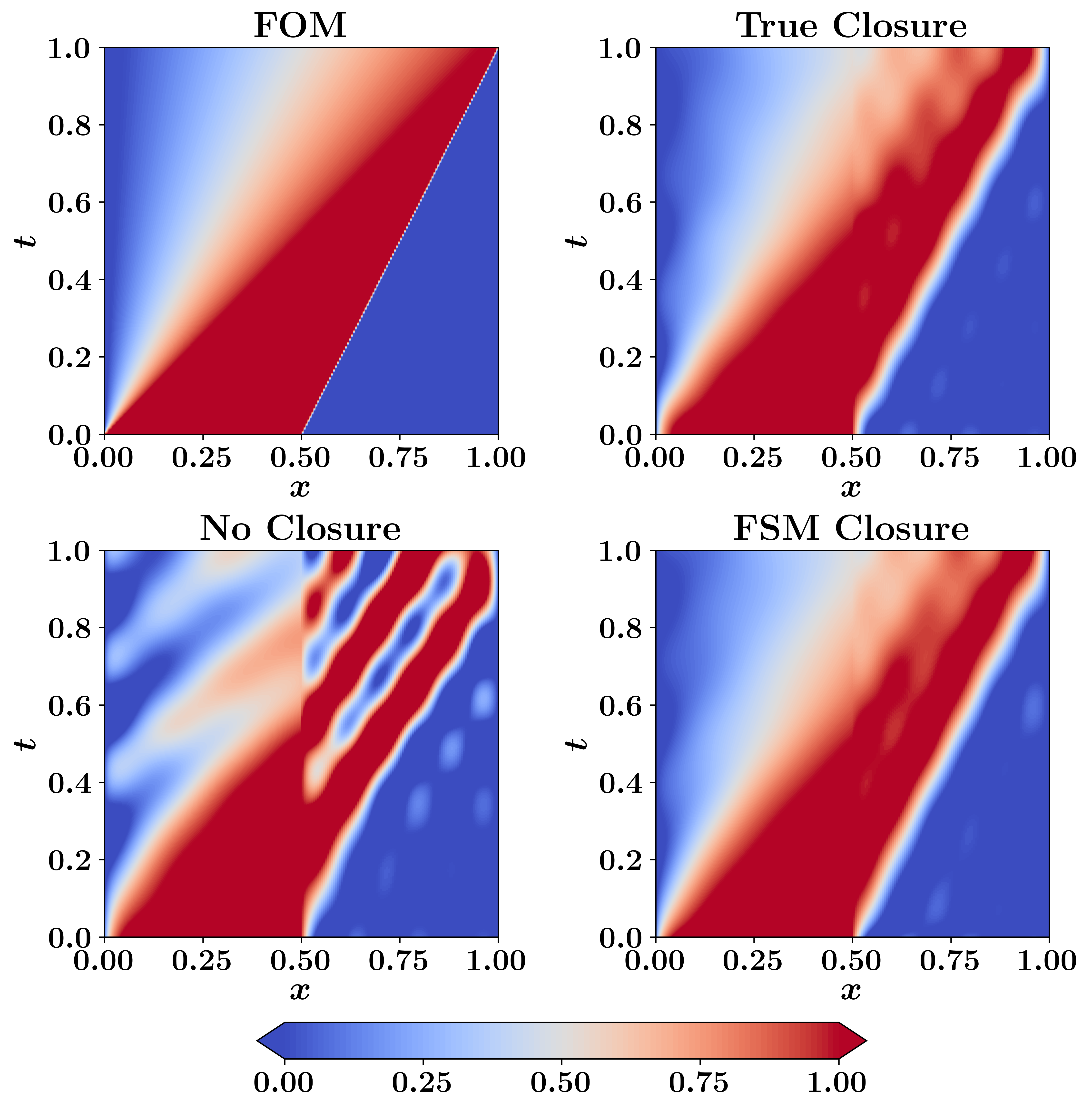
Figure 4: Spatio-temporal field predictions of Burgers problem using FOM and GROM approaches. Full field measurements are considered for the FSM Closure.

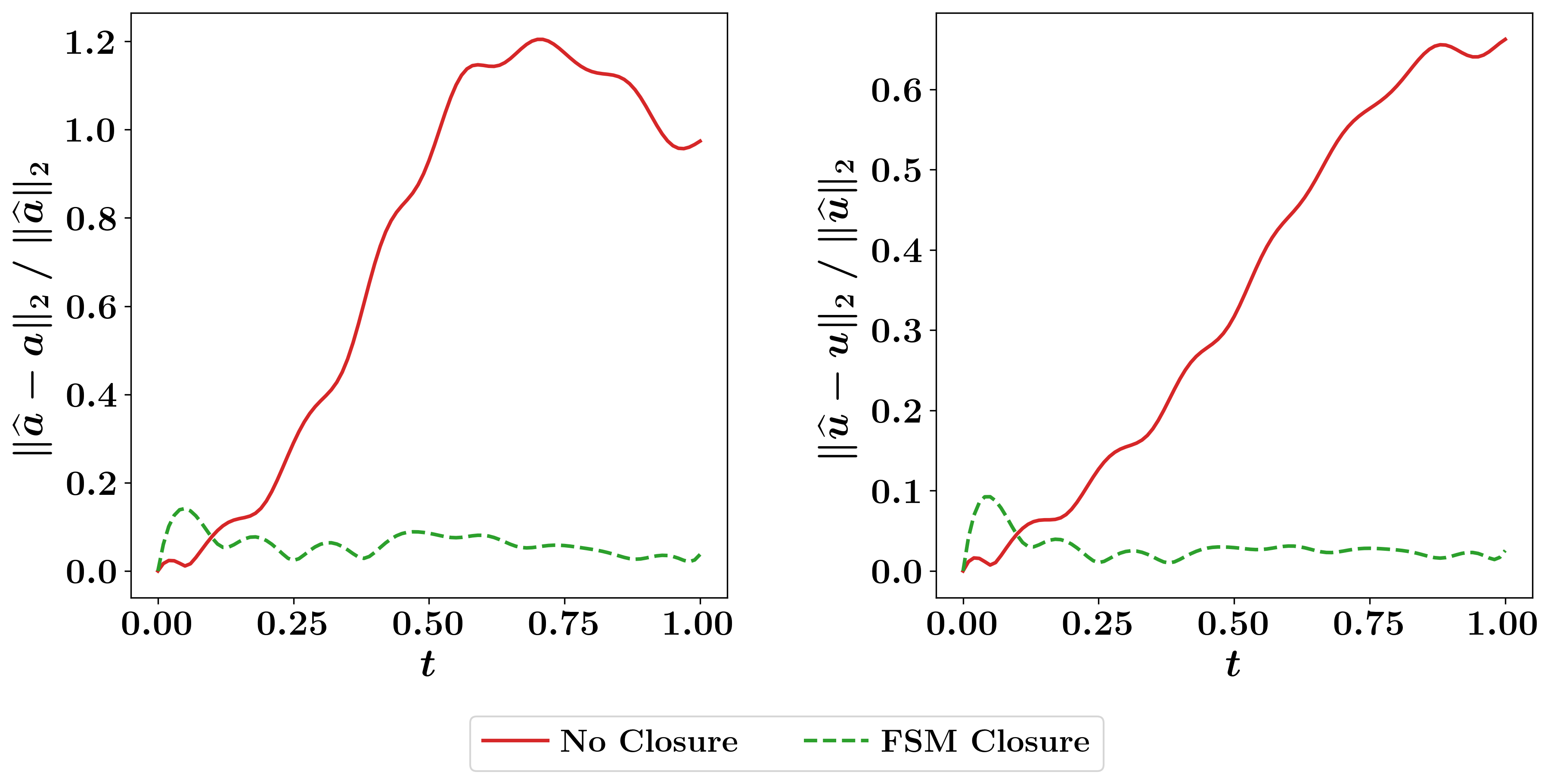
Figure 5: The relative error between the predicted values for the POD modal coefficients (left) and reconstructed velocity field (right) compared to their target values for 1D Burgers problem. Full field measurements are considered for the FSM Closure.

5.1.2 Sparse field observations

We extend our numerical experiments to explore incomplete field measurement scenarios. In particular, we consider a sparse signal $\boldsymbol{s}\in\mathbb{R}^{S}$ of the observable field $\boldsymbol{v}$ as follows:

$$\boldsymbol{s}=\boldsymbol{\Theta}\boldsymbol{v},$$ (41)

where $\boldsymbol{\Theta}\in\mathbb{R}^{S\times M}$ is a sampling matrix, constructed by taking $S$ rows of the $M\times M$ identity matrix (i.e., $[\boldsymbol{\Theta}]_{ij}=1$ if the $i^{th}$ sensor is located at the $j^{th}$ location and $[\boldsymbol{\Theta}]_{ij}=0$, otherwise). Sensors can be placed at equally-spaced locations, random locations, or carefully selected places.

Optimal sensor placement is an active field of research, also known as optimal experimental design (OED). We refer to [4] and references therein for more information. In this regard, we utilize a greedy compressed sensing algorithm based on QR decomposition with column pivoting to set-up a near-optimal sensor placement strategy as follows:

$$\boldsymbol{\Psi}^{T}\mathbf{P}:=\mathbf{Q}\mathbf{R},$$ (42)

where $\boldsymbol{\Psi}=[\boldsymbol{\psi}_{1},\boldsymbol{\psi}_{2},\dots,\boldsymbol{\psi}_{S}]\in\mathbb{R}^{M\times S}$ includes the first $S$ POD basis functions for $\boldsymbol{v}$, and $\mathbf{P}\in\mathbb{R}^{M\times M}$ is the permutation matrix. Manohar et al. [39] showed that by using the first $S$ rows of $\mathbf{P}$ to define the sampling matrix $\boldsymbol{\Theta}$, a near optimal sensor placement is obtained with similarities to the A- and D-optimality criteria in OED studies. Finally, the field $\boldsymbol{v}$ can be reconstructed as $\boldsymbol{v}\approx\boldsymbol{\Psi}(\boldsymbol{\Theta}\boldsymbol{\Psi})^{-1}\boldsymbol{s}$. Again, if we assume that the observable $\boldsymbol{v}$ is the velocity field $\boldsymbol{u}$ itself, the latent measurement $\boldsymbol{z}$ can be computed as $[\boldsymbol{z}(t)]_{i}=(\boldsymbol{\Psi}(\boldsymbol{\Theta}\boldsymbol{\Psi})^{-1}\boldsymbol{s}(t)-\bar{\boldsymbol{u}},\boldsymbol{\phi}_{i})$.

Figure 6 displays the time evolution of the first and sixth modal coefficients with the adopted FSM closure methodology in the case of sparse measurements. In particular, we selected $25$ locations (about $0.5\%$ of the total number of grid points) using the described QR-based algorithm to define the sensors data. We see that FSM closure yields very accurate results that are close to the the target trajectory even with the sparse measurement data. The reconstruction accuracy is also demonstrated using Fig. 7, showing significant improvements compared the GROM predictions without control. Similar observations can be found in Fig. 8 displaying the relative error for the predicted POD coefficients and the reconstructed velocity fields with respect to the target values that represent the minimum reconstruction error with $6$ modes.

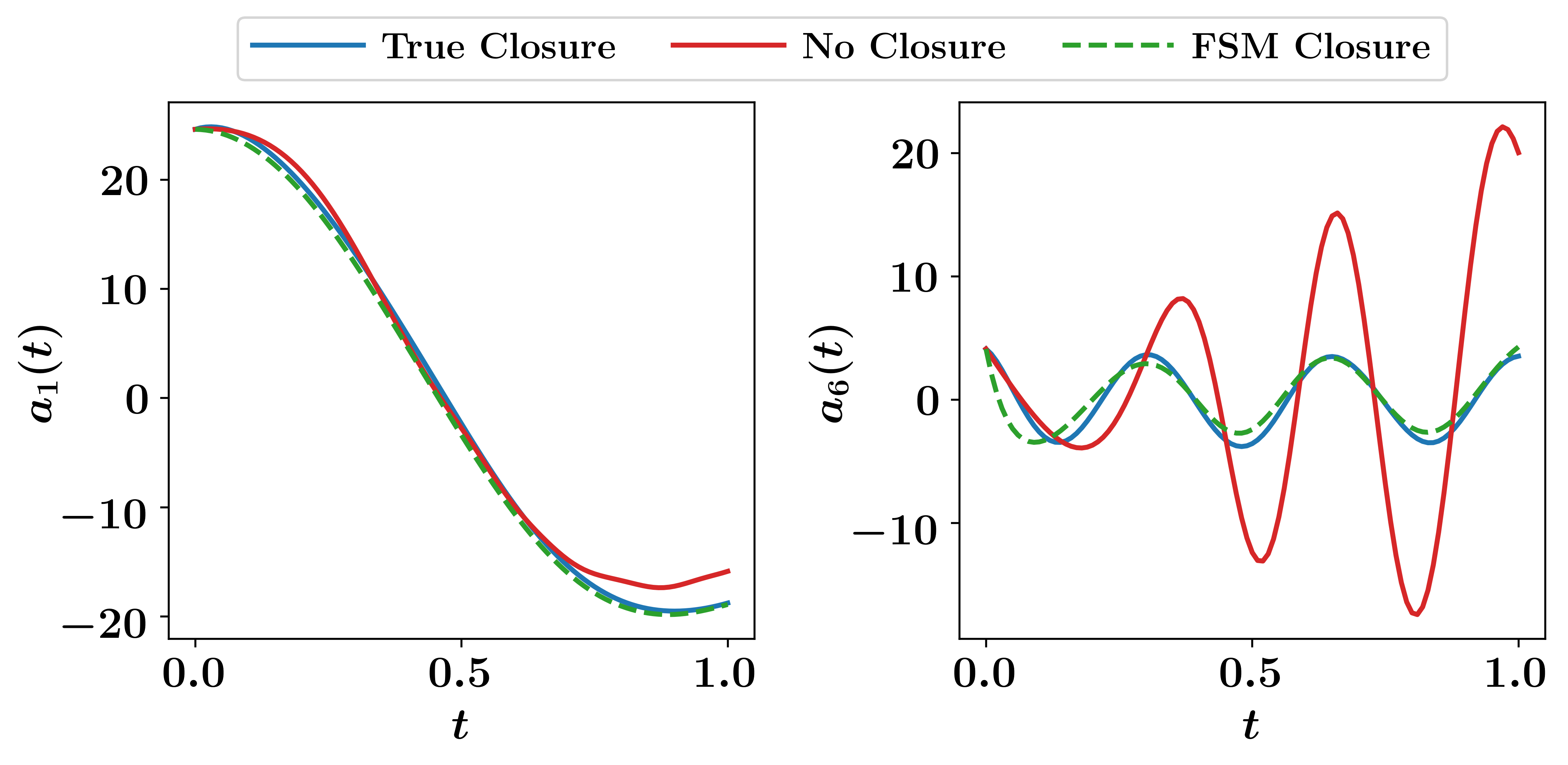
Figure 6: Dynamics of the first and last modal coefficients with sparse field measurement for the FSM Closure.

Figure 7: Spatio-temporal field predictions of Burgers problem using FOM and GROM approaches. Sparse field measurements are considered for the FSM Closure.

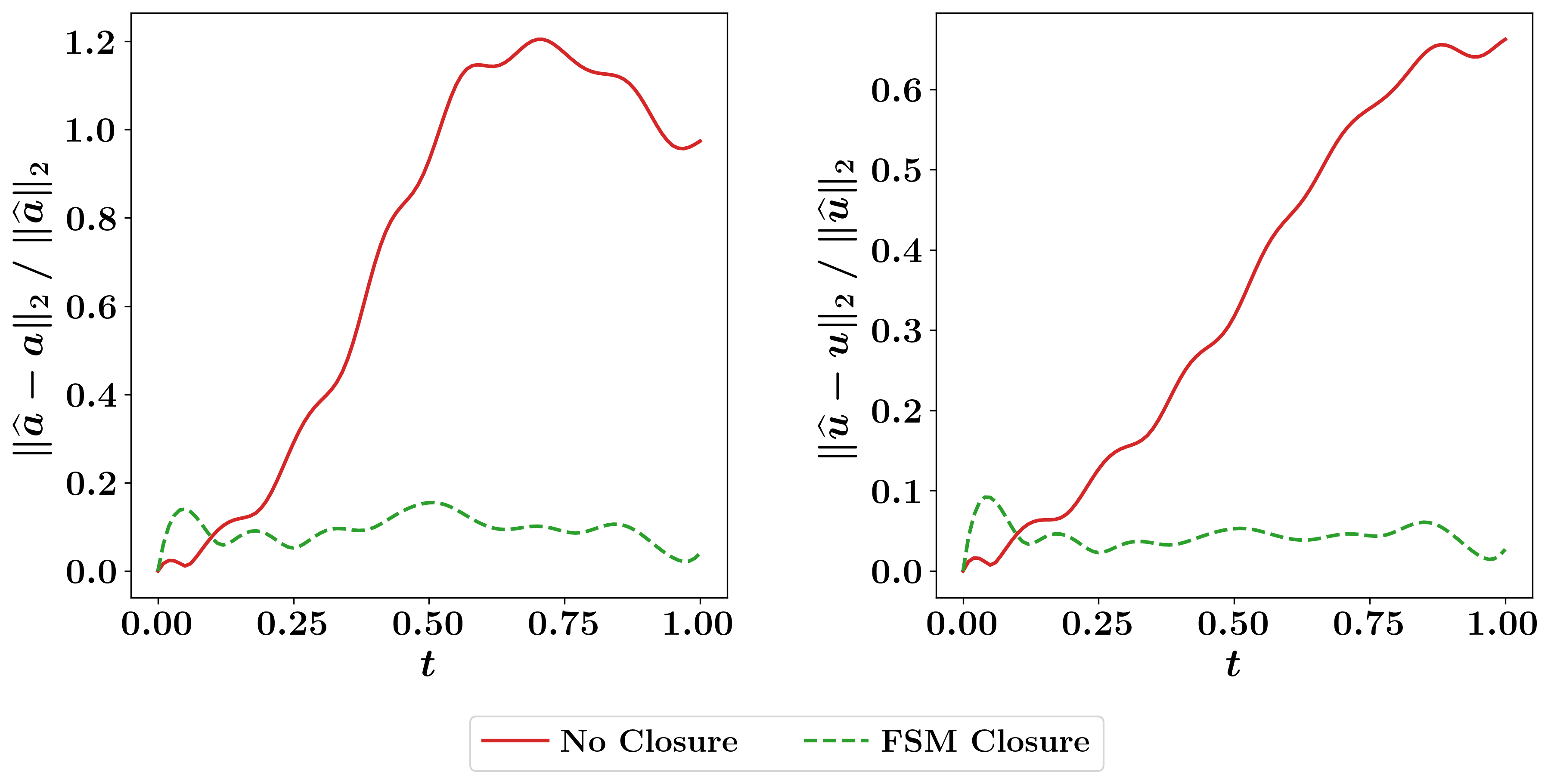
Figure 8: The relative error between the predicted values for the POD modal coefficients (left) and reconstructed velocity field (right) compared to their target values for 1D Burgers problem. Sparse field measurements are considered for the FSM Closure.

5.2 Vortex Merger Problem

One of the key benefits of the proposed FSM closure framework is that it is dealing with the reduced order model of the problem instead of the full fledged high dimensional model. Therefore, the computational complexity is dependent on the number of employed POD modes, rather than the spatial dimensionality of the problem. In order to highlight this aspect, we consider the two dimensional (2D) vortex merger problem [64], governed by the following vorticity transport equation:

$$\dfrac{\partial\omega}{\partial t}+J(\omega,\psi)=\dfrac{1}{\text{Re}}\Delta\omega,\qquad\text{in}\ \Omega\times[0,T].$$ (43)

where $\omega$ and $\psi$ denote the vorticity and streamfunction fields, and ($J(\cdot,\cdot)$) is the Jacobian operator defined as:

$$J(\omega,\psi) =\dfrac{\partial\omega}{\partial x}\dfrac{\partial\psi}{\partial y}-\dfrac{\partial\omega}{\partial y}\dfrac{\partial\psi}{\partial x}.$$ (44)

The vorticity and streamfunction are linked by the kinematic relationship:

$$\Delta\psi=-\omega.$$ (45)

We consider a spatial domain of dimensions $(2\pi\times 2\pi)$ with periodic boundary conditions in both the $x$ and $y$ directions. The flow is initiated with a pair of co-rotating Gaussian vortices with equal strengths centered at $(x_{1},y_{1})=(5\pi/4,\pi)$ and $(x_{2},y_{2})=(3\pi/4,\pi)$ as follows:

$$\omega(x,y,0)=\exp\left(-\rho\left[(x-x_{1})^{2}+(y-y_{1})^{2}\right]\right)+\exp{\left(-\rho\left[(x-x_{2})^{2}+(y-y_{2})^{2}\right]\right)},$$ (46)

where $\rho$ is a parameter that controls the mutual interactions between the two vortical motions. In the present study, we consider $\text{Re}=5000$ and set $\rho=\pi$. For the FOM simulations, we define a regular Cartesian grid with a resolution of $256\times 256$ (i.e., $\Delta x=\Delta y=2\pi/256$). For temporal integration of the FOM model, we use the TVD-RK3 scheme with a time-step of $10^{-3}$. Vorticity snapshots are collected every 100 time-steps for $t\in[0,50]$, resulting in a total of $500$ snapshots. The evolution of the vortex merger problem is depicted in Fig. 9, which illustrates the convective and interactive mechanisms affecting the transport and development of the two vortices. This makes it a challenging problem for standard ROM approaches and a good test bed for the proposed FSM framework.

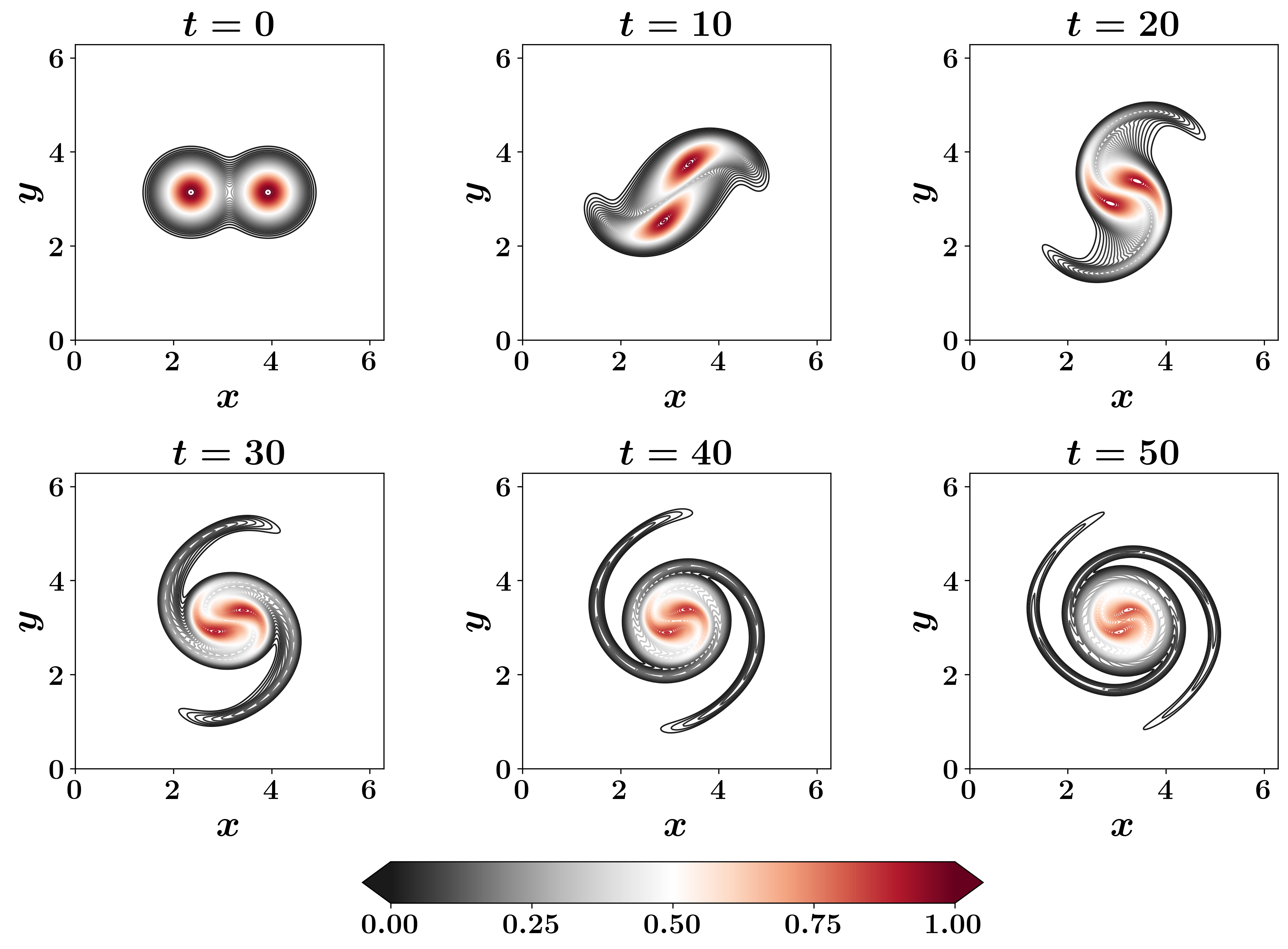
Figure 9: Samples of temporal snapshots of the vorticity field for the vortex merger problem at $\text{Re}=5000$.

In terms of POD analysis, we use $n=6$ to define the total number of resolved scales and hence the dimensionality of the GROM system. The decay of the POD eigenvalue and the RIC values for the current setup is shown in Fig. 10. Finally, the GROM terms for the vortex merger problem can be written as follows:

_k $$=\bigg{(}-J(\bar{\omega},\bar{\psi})+\dfrac{1}{\text{Re}}\nabla^{2}\bar{\omega},\boldsymbol{\phi}_{k}^{\omega}\bigg{)},$$ (47)

$$[\boldsymbol{L}]_{k,i} =\bigg{(}-J(\bar{\omega},\boldsymbol{\phi}_{i}^{\psi})-J(\boldsymbol{\phi}_{i}^{\omega},\bar{\psi})+\dfrac{1}{\text{Re}}\Delta\phi_{i}^{\omega},\boldsymbol{\phi}_{k}^{\omega}\bigg{)},$$

$$[\boldsymbol{N}]_{k,i,j} =\bigg{(}-J(\boldsymbol{\phi}_{i}^{\omega},\boldsymbol{\phi}_{j}^{\psi});\boldsymbol{\phi}_{k}^{\omega}\bigg{)}.$$

Similar to Eq. 39, we modify Eq. 43 to derive the closure model as follows:

$$\dfrac{\partial\omega}{\partial t}+J(\omega,\psi)=\dfrac{1}{\text{Re}}\Delta\omega+\gamma\omega+\beta\Delta\omega,$$ (48)

which results in the following terms for the closure model in Eq. 17:

$$[\boldsymbol{e}]_{k}=\big{(}\bar{\omega},\boldsymbol{\phi}_{k}\big{)},\qquad[\boldsymbol{q}]_{k}=\big{(}\Delta\bar{\omega},\boldsymbol{\phi}_{k}\big{)},\qquad[\boldsymbol{D}]_{k,i}=\big{(}\Delta\boldsymbol{\phi}_{i},\boldsymbol{\phi}_{k}\big{)}.$$ (49)

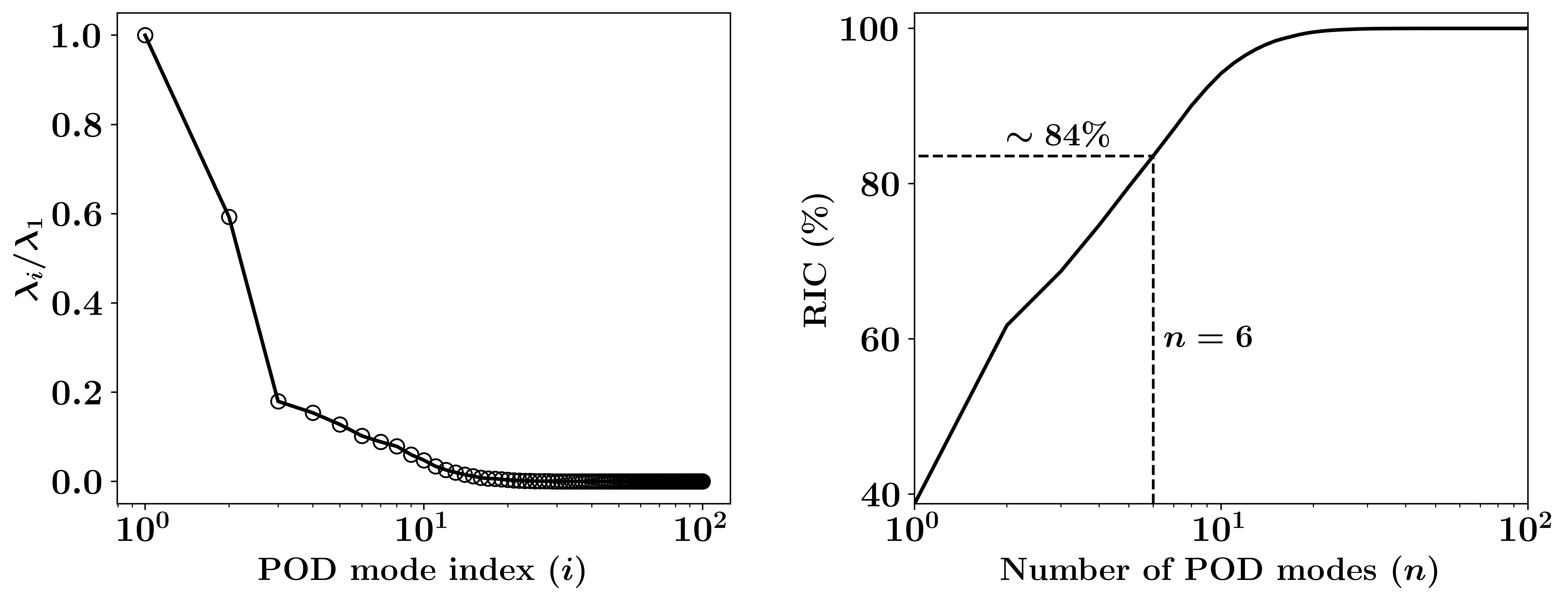
Figure 10: The decay of eigenvalues (left) and behavior of relative information content (right) for the 2D vortex merger problem at $\text{Re}=5000$.

5.2.1 Full field observations

We first explore the idealized case where full field measurements of the vorticity fields are collected. We also consider additive Gaussian noise with zero mean and standard deviation of $0.1$. We record data every $5$ time units, corresponding to a total of $10$ measurement instants. We apply the approach presented in Section 4 to compute the mode-dependent parameters $\gamma_{i}$ and $\beta_{i}$ for $i=1,2,\dots,n$. The estimated parameters values are then plugged into Eq. 17 to define the closure model. The corresponding predictions of the POD modal coefficients are shown in Fig. 11, where we see that the higher amplitude oscillations are damped and the ROM trajectory is getting closer to the target values.

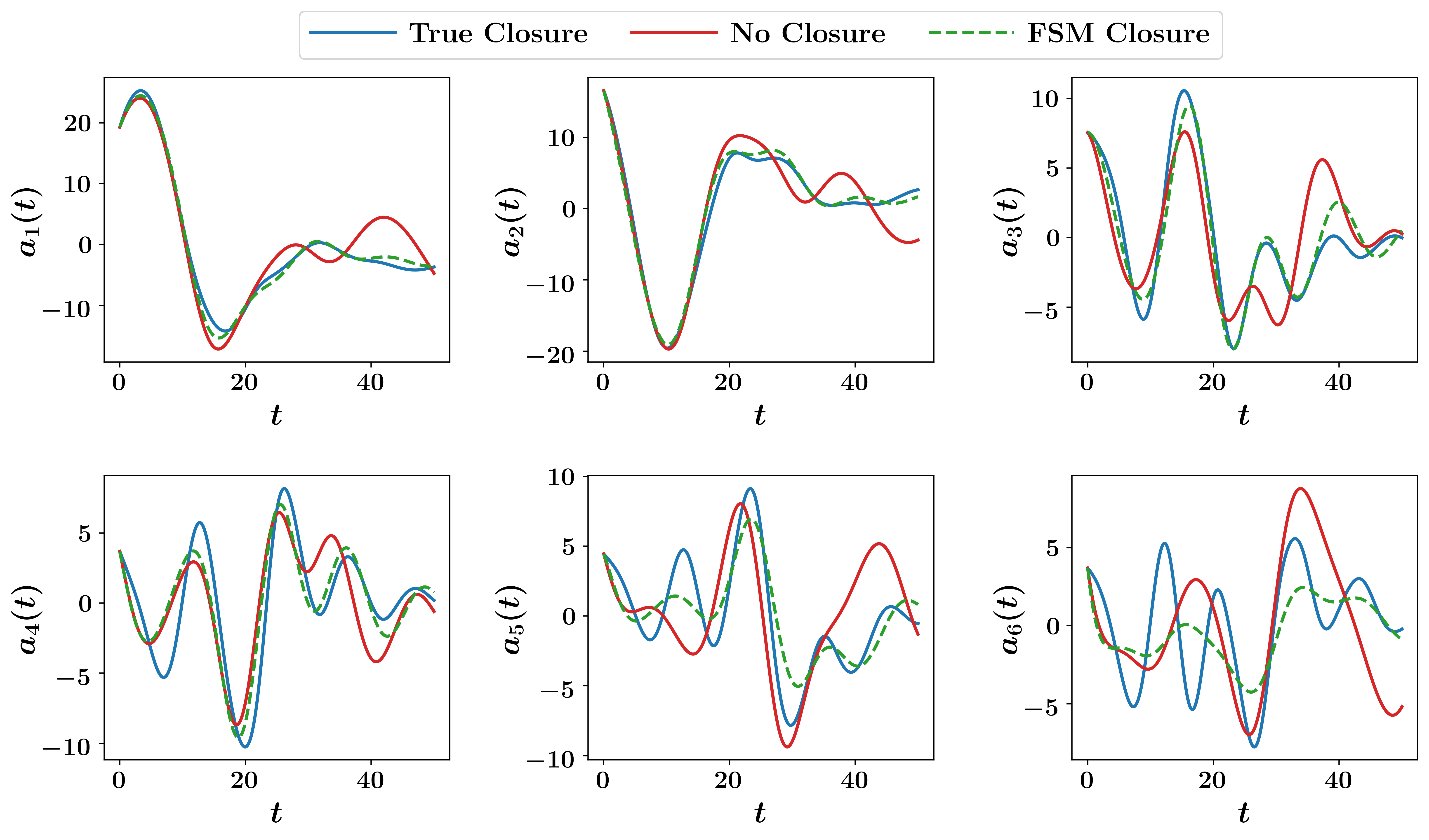
Figure 11: The time evolution of the first 6 modes of the vortex merger problem when full field measurements are collected every $5$ time units.

In addition, the reconstruction of the vorticity field at two different time instants is depicted in Fig. 12. We see that the GROM model without closure results in flow field predictions that miss significant flow features. On the other hand, the FSM Closure framework is capable of parameterizing the latent control model resulting in a reduced reconstruction error. Figure 13 also shows the relative error for the predicted POD coefficients as well as the reconstructed vorticity fields as a function of time.

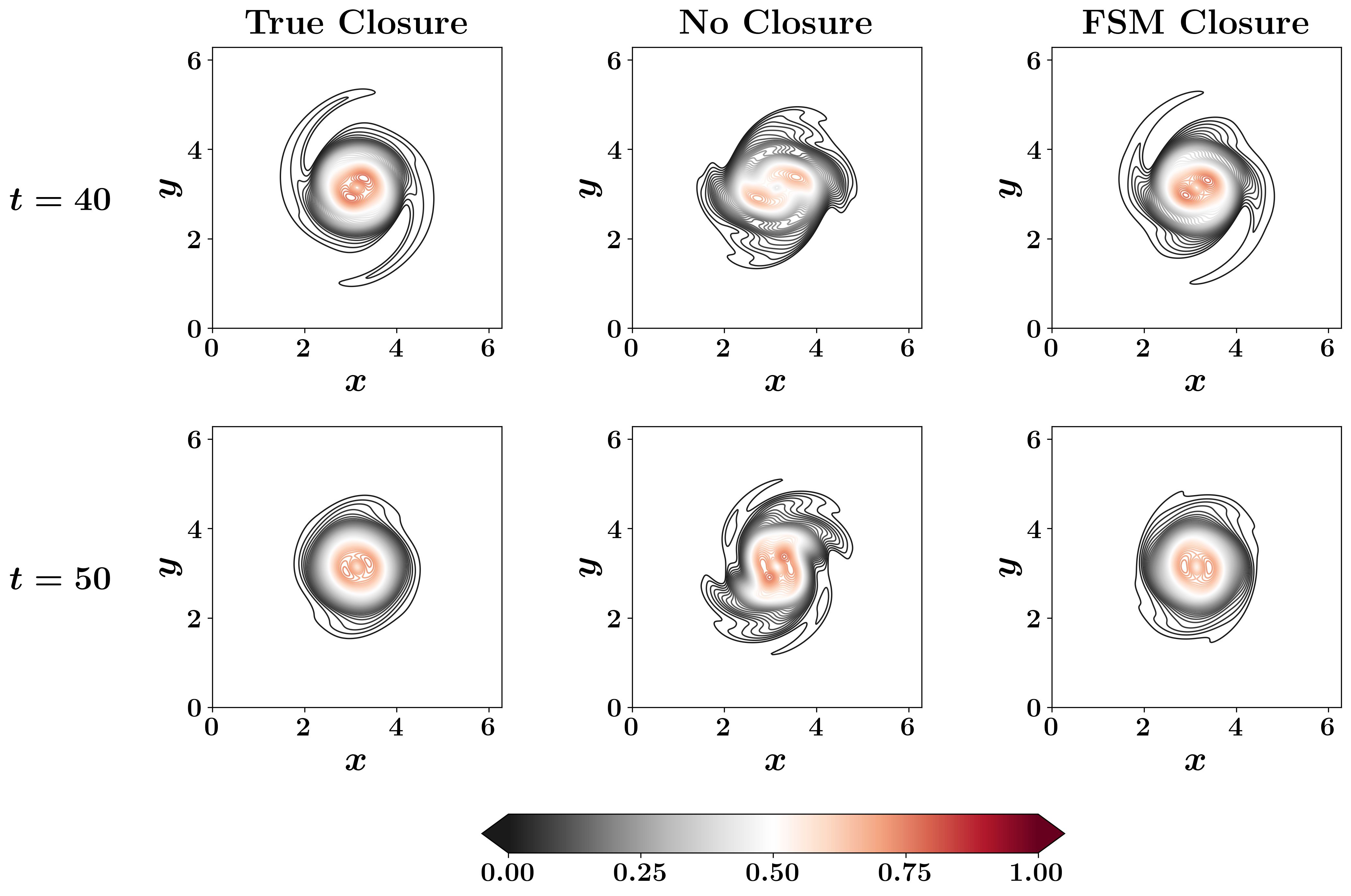
Figure 12: Comparison between the vorticity field at the $t=40$ (top) and $t=50$ (bottom) with True Closure (ground truth from FOM data), No Closure (standard GROM) and the proposed FSM Closure approach with full field measurements.

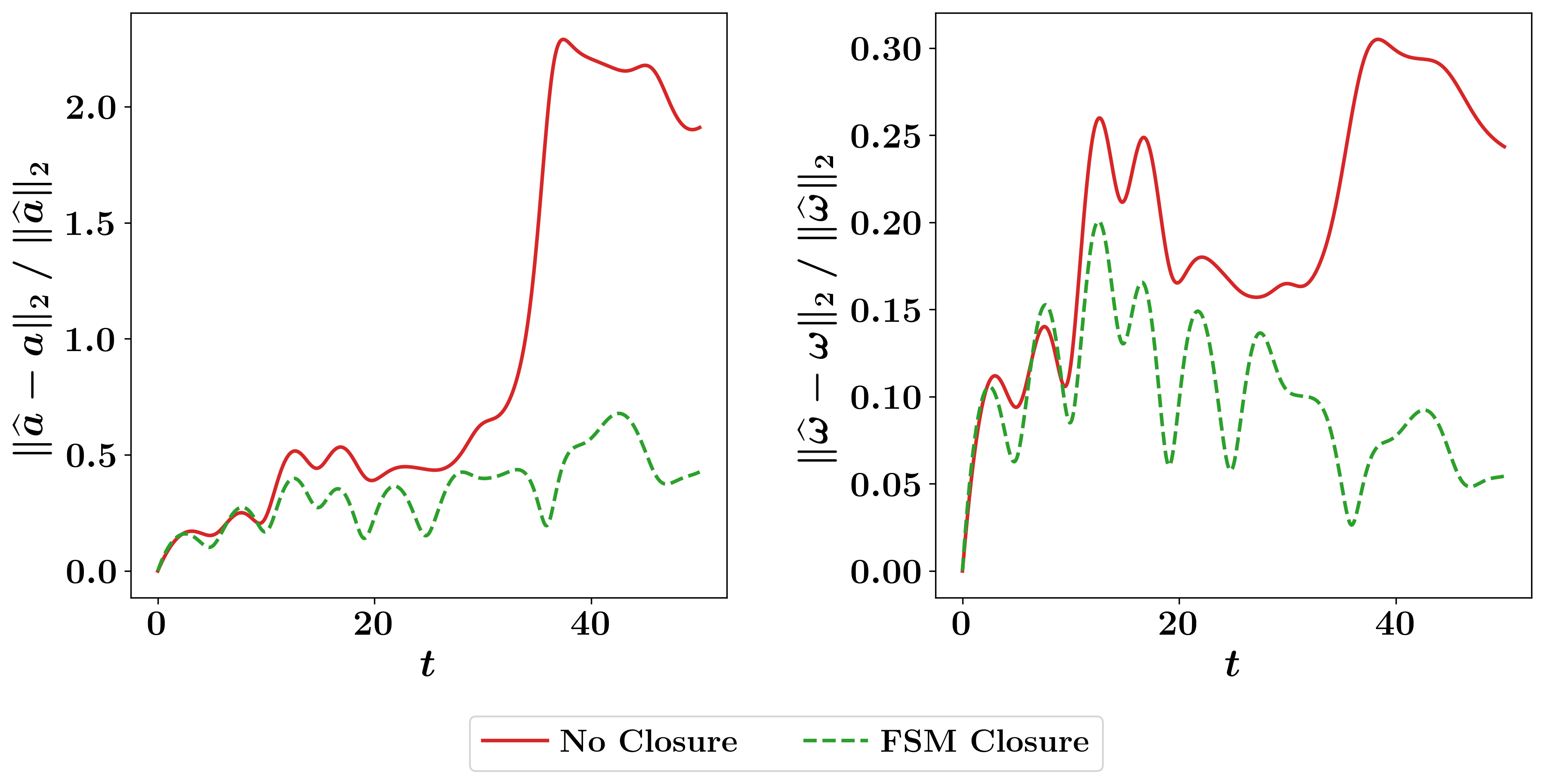
Figure 13: The relative error between the predicted values for the POD modal coefficients (left) and reconstructed vorticity field (right) compared to their target values for 2D vortex merger problem. Full field measurements are considered for the FSM Closure.

5.2.2 Sparse field observations

In this section, we investigate the performance of the proposed forward sensitivity approach for mode-dependent control when only spatially sparse observations are available. In particular, we consider a relatively data-scarce regime with $25$ spatial locations (that is less than $0.04\%$ of the total number of grid points). We also incorporate additive Gaussian noise similar to Section 5.2.1. Although it is typically possible to clean this data a bit by considering its spectrum, we intentionally avoid this step to assess the robustness of the FSM framework to data noise and sparsity. We illustrate the predictions of the system’s dynamics in the latent space in Fig. 14. As expected, the predictions of the GROM with FSM closure is quite less accurate than the case with full field measurements (i.e., Fig. 11) especially at later times. However, compared to the uncontrolled GROM model, we see that the FSM Closure introduces substantial improvements.

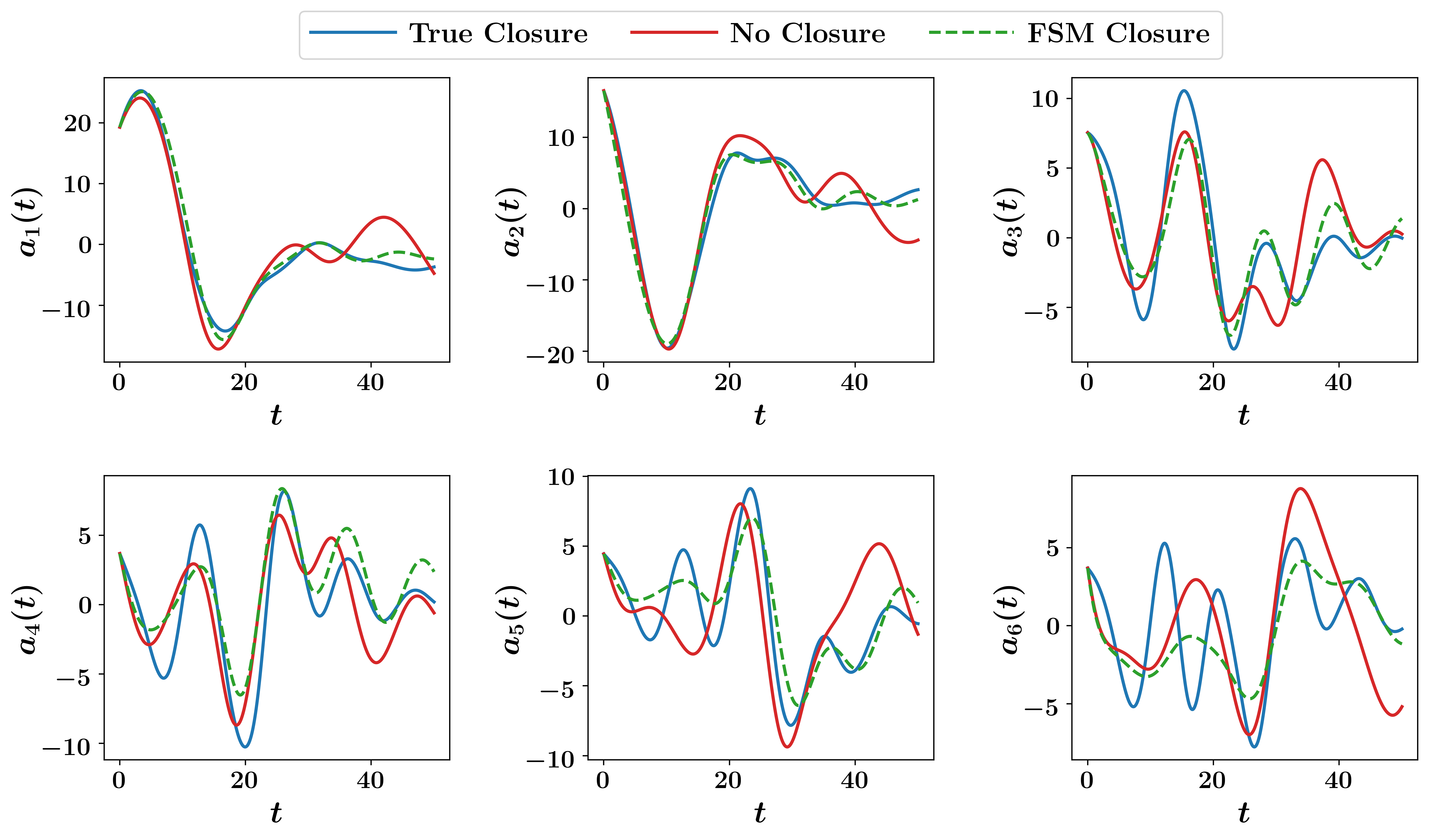
Figure 14: The time evolution of the first 6 modes of the vortex merger problem when only sparse field measurements are available.

We also observe that the predictions of the first few modes is closer to the target values than the peredictions of the last modes (e.g., $a_{5}$ and $a_{6}$). This can be explained by the principle of locality of energy transfer (and modal interactions) of the variational multiscale method [43, 2]. It implies that the POD truncation results in a model that has much less information about the modes that are closer to the cut-off (e.g., the latest modes) than those that are farther away from the cut-off (e.g., the first modes). In addition, since the first modes have larger contribution to the data construction, the FSM algorithm tends to give higher importance to those mode as it minimizes the error with respect to the measurements. One way to address this issue could be to define a different scaling to ensure that all modal coefficient are equally important. We also show the reconstructed vorticity fields from the GROM without closure as well as GROM with FSM closure at $t=40$ and $t=50$ in Fig. 15. We observe that the FSM closure results in a more accurate recovery of the underlying flow features with respect to the target values (denoted as True Closure). Finally, Fig. 16 shows the relative error for the predicted POD coefficients as well as the reconstructed vorticity fields as a function of time.

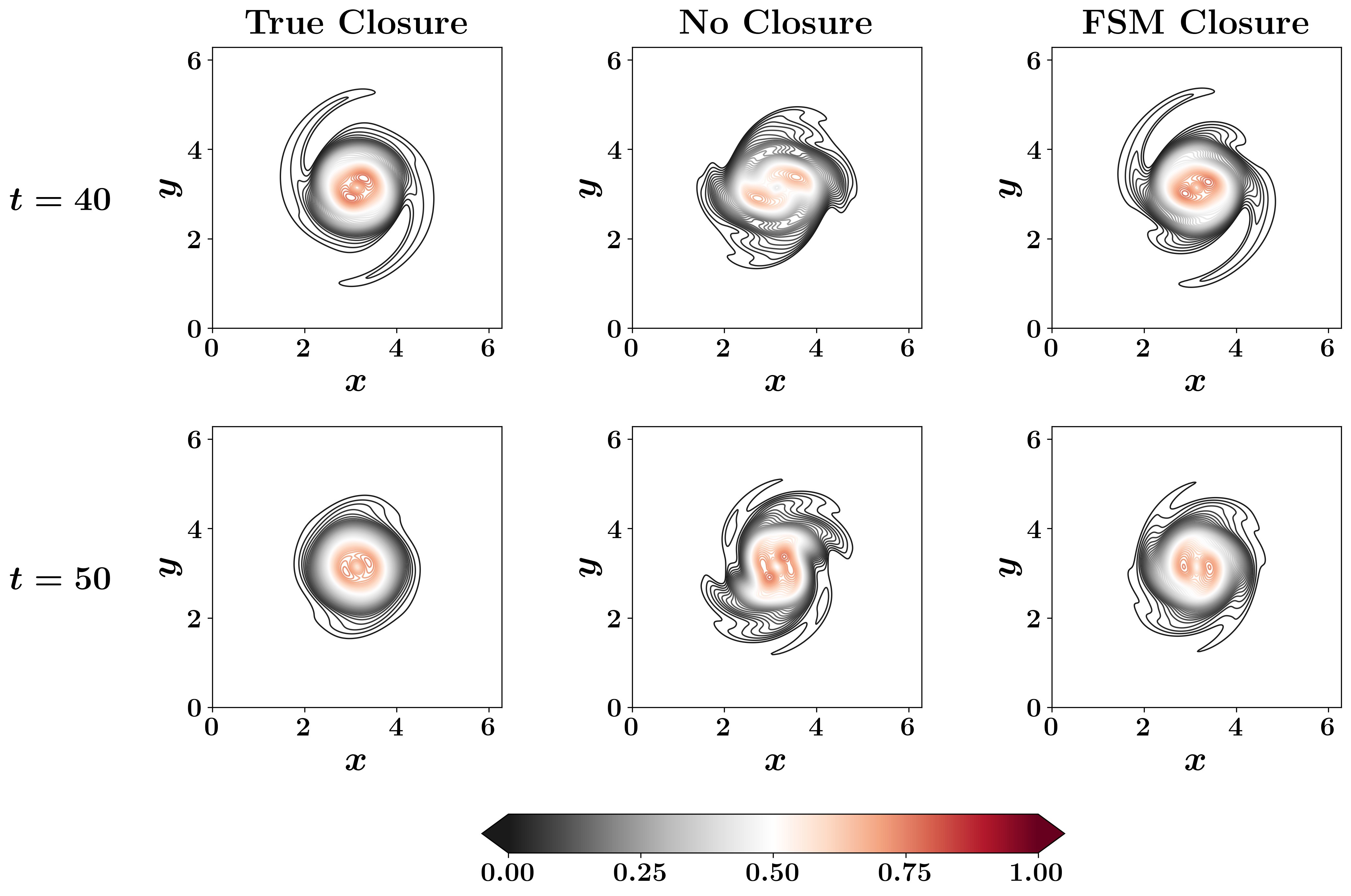
Figure 15: Comparison between the vorticity field at the $t=40$ (top) and $t=50$ (bottom) with True Closure (ground truth from FOM data), No Closure (standard GROM) and the proposed FSM Closure approach with sparse field measurements.

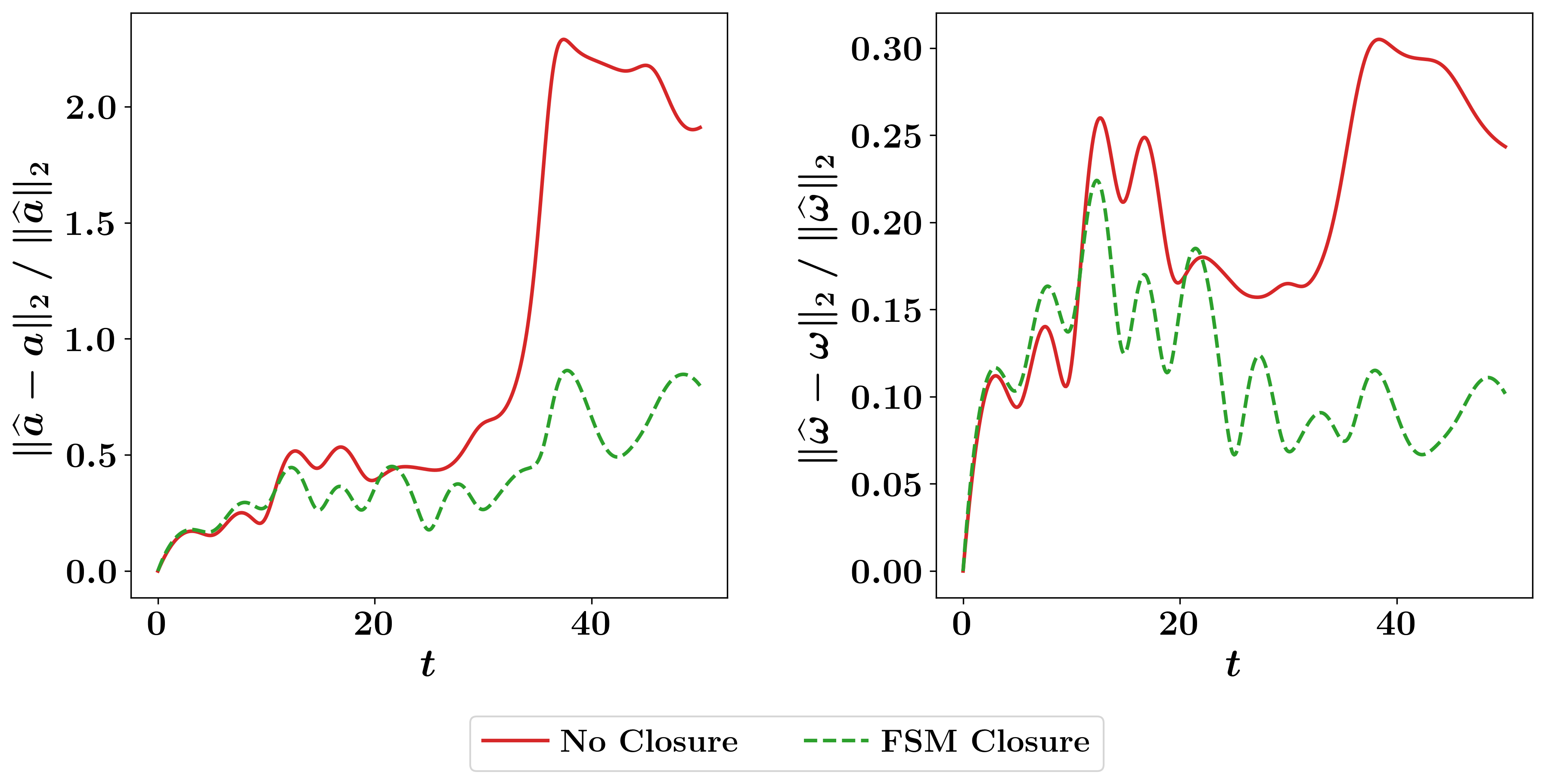
Figure 16: The relative error between the predicted values for the POD modal coefficients (left) and reconstructed vorticity field (right) compared to their target values for 2D vortex merger problem. Sparse field measurements are considered for the FSM Closure.

6 Concluding Remarks

We propose a variational approach for correcting nonlinear reduced order models (ROMs) using the forward sensitivity method (FSM). We cast the closure as a control input in the latent space of the ROM and utilize physical arguments to build parameterized models with damping and dissipation terms. We leverage FSM to blend the predictions from the ROM with available sparse and noisy observations to estimate the unknown model parameters. We apply this approach on a projection based ROM of two test problems with varying complexity corresponding to the one dimensional viscous Burgers equation and the two dimensional vortex-merger problem. These are often considered as canonical test beds for broad transport phenomena governed by nonlinear partial differential equations. We investigate the capability of the approach to approximate optimal values for the mode-dependent parameters without constraining the direction of energy transfer between different modes. Results show that equipping GROM with FSM-based control dramatically increases the ROM accuracy. The predicted trajectories get closer to the values that provide the minimum reconstruction error. The presented framework can effectively enhance digital twin technologies where computationally-light models are required and sensor data are continuously collected.

Data Availability

The synthetic data that support the findings of this study are available within the article. The complete list of Python scripts that are used in this study can be found in the GitHub page: https://github.com/Shady-Ahmed/fsm-rom-control.

References

- Ahmed et al. [2021] Ahmed, S.E., Pawar, S., San, O., Rasheed, A., Iliescu, T., Noack, B.R., 2021. On closures for reduced order models—a spectrum of first-principle to machine-learned avenues. Physics of Fluids 33, 091301.
- Ahmed et al. [2022] Ahmed, S.E., San, O., Rasheed, A., Iliescu, T., Veneziani, A., 2022. Physics guided machine learning for variational multiscale reduced order modeling. arXiv preprint arXiv:2205.12419 .
- Akhtar et al. [2012] Akhtar, I., Wang, Z., Borggaard, J., Iliescu, T., 2012. A new closure strategy for proper orthogonal decomposition reduced-order models. Journal of Computational and Nonlinear Dynamics 7.
- Alexanderian [2021] Alexanderian, A., 2021. Optimal experimental design for infinite-dimensional bayesian inverse problems governed by PDEs: A review. Inverse Problems 37, 043001.
- Aubry [1991] Aubry, N., 1991. On the hidden beauty of the proper orthogonal decomposition. Theoretical and Computational Fluid Dynamics 2, 339–352.
- Balajewicz et al. [2016] Balajewicz, M., Tezaur, I., Dowell, E., 2016. Minimal subspace rotation on the stiefel manifold for stabilization and enhancement of projection-based reduced order models for the compressible navier–stokes equations. Journal of Computational Physics 321, 224–241.
- Benosman [2018] Benosman, M., 2018. Model-based vs data-driven adaptive control: an overview. International Journal of Adaptive Control and Signal Processing 32, 753–776.
- Benosman et al. [2017] Benosman, M., Borggaard, J., San, O., Kramer, B., 2017. Learning-based robust stabilization for reduced-order models of 2d and 3d boussinesq equations. Applied Mathematical Modelling 49, 162–181.
- Bergmann et al. [2009] Bergmann, M., Bruneau, C.H., Iollo, A., 2009. Enablers for robust POD models. Journal of Computational Physics 228, 516–538.
- Berkooz et al. [1993] Berkooz, G., Holmes, P., Lumley, J.L., 1993. The proper orthogonal decomposition in the analysis of turbulent flows. Annual Review of Fluid Mechanics 25, 539–575.
- Beucler et al. [2021] Beucler, T., Pritchard, M., Rasp, S., Ott, J., Baldi, P., Gentine, P., 2021. Enforcing analytic constraints in neural networks emulating physical systems. Physical Review Letters 126, 098302.
- Borggaard et al. [2011] Borggaard, J., Iliescu, T., Wang, Z., 2011. Artificial viscosity proper orthogonal decomposition. Mathematical and Computer Modelling 53, 269–279.
- Brunton and Noack [2015] Brunton, S.L., Noack, B.R., 2015. Closed-loop turbulence control: Progress and challenges. Applied Mechanics Reviews 67.
- Cazemier et al. [1998] Cazemier, W., Verstappen, R., Veldman, A., 1998. Proper orthogonal decomposition and low-dimensional models for driven cavity flows. Physics of Fluids 10, 1685–1699.
- Chakraborty [2021] Chakraborty, S., 2021. Transfer learning based multi-fidelity physics informed deep neural network. Journal of Computational Physics 426, 109942.
- Cordier et al. [2013] Cordier, L., Noack, B.R., Tissot, G., Lehnasch, G., Delville, J., Balajewicz, M., Daviller, G., Niven, R.K., 2013. Identification strategies for model-based control. Experiments in Fluids 54, 1–21.
- Cuomo et al. [2022] Cuomo, S., Di Cola, V.S., Giampaolo, F., Rozza, G., Raissi, M., Piccialli, F., 2022. Scientific machine learning through physics-informed neural networks: Where we are and what’s next. arXiv preprint arXiv:2201.05624 .
- Dada and Armaou [2020] Dada, G.P., Armaou, A., 2020. Generalized SVD reduced-order observers for nonlinear systems, in: 2020 American Control Conference (ACC), IEEE. pp. 3473–3478.
- De et al. [2020] De, S., Britton, J., Reynolds, M., Skinner, R., Jansen, K., Doostan, A., 2020. On transfer learning of neural networks using bi-fidelity data for uncertainty propagation. International Journal for Uncertainty Quantification 10.
- Eroglu et al. [2017] Eroglu, F.G., Kaya, S., Rebholz, L.G., 2017. A modular regularized variational multiscale proper orthogonal decomposition for incompressible flows. Comput. Meth. Appl. Mech. Eng. 325, 350–368.
- Garg et al. [2022] Garg, S., Chakraborty, S., Hazra, B., 2022. Physics-integrated hybrid framework for model form error identification in nonlinear dynamical systems. Mechanical Systems and Signal Processing 173, 109039.
- Giere et al. [2015] Giere, S., Iliescu, T., John, V., Wells, D., 2015. SUPG reduced order models for convection-dominated convection–diffusion–reaction equations. Computer Methods in Applied Mechanics and Engineering 289, 454–474.
- Goswami et al. [2020] Goswami, S., Anitescu, C., Chakraborty, S., Rabczuk, T., 2020. Transfer learning enhanced physics informed neural network for phase-field modeling of fracture. Theoretical and Applied Fracture Mechanics 106, 102447.
- Greydanus et al. [2019] Greydanus, S., Dzamba, M., Yosinski, J., 2019. Hamiltonian neural networks. arXiv preprint arXiv:1906.01563 .
- Grimberg et al. [2020] Grimberg, S., Farhat, C., Youkilis, N., 2020. On the stability of projection-based model order reduction for convection-dominated laminar and turbulent flows. Journal of Computational Physics 419, 109681.
- Holmes et al. [2012] Holmes, P., Lumley, J.L., Berkooz, G., Rowley, C.W., 2012. Turbulence, coherent structures, dynamical systems and symmetry. Cambridge University Press.
- Huang and Kramer [2020] Huang, Y., Kramer, B., 2020. Balanced reduced-order models for iterative nonlinear control of large-scale systems. IEEE Control Systems Letters 5, 1699–1704.
- Iliescu and Wang [2014] Iliescu, T., Wang, Z., 2014. Variational multiscale proper orthogonal decomposition: Navier-stokes equations. Numerical Methods for Partial Differential Equations 30, 641–663.
- Ivagnes et al. [2022] Ivagnes, A., Demo, N., Rozza, G., 2022. Towards a machine learning pipeline in reduced order modelling for inverse problems: neural networks for boundary parametrization, dimensionality reduction and solution manifold approximation. arXiv preprint arXiv:2210.14764 .
- Karniadakis et al. [2021] Karniadakis, G.E., Kevrekidis, I.G., Lu, L., Perdikaris, P., Wang, S., Yang, L., 2021. Physics-informed machine learning. Nature Reviews Physics 3, 422–440.
- Kashinath et al. [2021] Kashinath, K., Mustafa, M., Albert, A., Wu, J., Jiang, C., Esmaeilzadeh, S., Azizzadenesheli, K., Wang, R., Chattopadhyay, A., Singh, A., et al., 2021. Physics-informed machine learning: case studies for weather and climate modelling. Philosophical Transactions of the Royal Society A 379, 20200093.
- Koc et al. [2022] Koc, B., Mou, C., Liu, H., Wang, Z., Rozza, G., Iliescu, T., 2022. Verifiability of the data-driven variational multiscale reduced order model. Journal of Scientific Computing 93, 1–26.
- Kramer et al. [2017] Kramer, B., Grover, P., Boufounos, P., Nabi, S., Benosman, M., 2017. Sparse sensing and DMD-based identification of flow regimes and bifurcations in complex flows. SIAM Journal on Applied Dynamical Systems 16, 1164–1196.
- Kravaris [2016] Kravaris, C., 2016. Functional observers for nonlinear systems. IFAC-PapersOnLine 49, 505–510.
- Lakshmivarahan and Lewis [2010] Lakshmivarahan, S., Lewis, J.M., 2010. Forward sensitivity approach to dynamic data assimilation. Advances in Meteorology 2010.
- Lakshmivarahan et al. [2017] Lakshmivarahan, S., Lewis, J.M., Jabrzemski, R., 2017. Forecast error correction using dynamic data assimilation. Springer, New York.
- Lassila et al. [2014] Lassila, T., Manzoni, A., Quarteroni, A., Rozza, G., 2014. Model order reduction in fluid dynamics: challenges and perspectives. Reduced Order Methods for modeling and computational reduction , 235–273.
- Ling et al. [2016] Ling, J., Kurzawski, A., Templeton, J., 2016. Reynolds averaged turbulence modelling using deep neural networks with embedded invariance. Journal of Fluid Mechanics 807, 155–166.
- Manohar et al. [2018] Manohar, K., Brunton, B.W., Kutz, J.N., Brunton, S.L., 2018. Data-driven sparse sensor placement for reconstruction: Demonstrating the benefits of exploiting known patterns. IEEE Control Systems Magazine 38, 63–86.
- Maulik et al. [2019] Maulik, R., San, O., Rasheed, A., Vedula, P., 2019. Subgrid modelling for two-dimensional turbulence using neural networks. Journal of Fluid Mechanics 858, 122–144.
- Meng and Karniadakis [2020] Meng, X., Karniadakis, G.E., 2020. A composite neural network that learns from multi-fidelity data: Application to function approximation and inverse PDE problems. Journal of Computational Physics 401, 109020.
- Mohan et al. [2020] Mohan, A.T., Lubbers, N., Livescu, D., Chertkov, M., 2020. Embedding hard physical constraints in neural network coarse-graining of 3D turbulence. arXiv preprint arXiv:2002.00021 .
- Mou et al. [2021] Mou, C., Koc, B., San, O., Rebholz, L.G., Iliescu, T., 2021. Data-driven variational multiscale reduced order models. Computer Methods in Applied Mechanics and Engineering 373, 113470.
- Niazi et al. [2019] Niazi, M.U.B., Deplano, D., Canudas-de Wit, C., Kibangou, A.Y., 2019. Scale-free estimation of the average state in large-scale systems. IEEE Control Systems Letters 4, 211–216.
- Noack et al. [2011] Noack, B.R., Morzynski, M., Tadmor, G., 2011. Reduced-Order Modelling for Flow Control. volume 528. Springer-Verlag, Berlin.
- Novati et al. [2021] Novati, G., de Laroussilhe, H.L., Koumoutsakos, P., 2021. Automating turbulence modelling by multi-agent reinforcement learning. Nature Machine Intelligence 3, 87–96.
- Pacciarini and Rozza [2014] Pacciarini, P., Rozza, G., 2014. Stabilized reduced basis method for parametrized advection–diffusion pdes. Computer Methods in Applied Mechanics and Engineering 274, 1–18.
- Papapicco et al. [2022] Papapicco, D., Demo, N., Girfoglio, M., Stabile, G., Rozza, G., 2022. The neural network shifted-proper orthogonal decomposition: A machine learning approach for non-linear reduction of hyperbolic equations. Computer Methods in Applied Mechanics and Engineering 392, 114687.
- Pastoor et al. [2008] Pastoor, M., Henning, L., Noack, B.R., King, R., Tadmor, G., 2008. Feedback shear layer control for bluff body drag reduction. Journal of fluid mechanics 608, 161–196.
- Pawar and San [2022] Pawar, S., San, O., 2022. Equation-free surrogate modeling of geophysical flows at the intersection of machine learning and data assimilation. arXiv preprint arXiv:2205.13410 .
- Pawar et al. [2021a] Pawar, S., San, O., Aksoylu, B., Rasheed, A., Kvamsdal, T., 2021a. Physics guided machine learning using simplified theories. Physics of Fluids 33, 011701.
- Pawar et al. [2021b] Pawar, S., San, O., Nair, A., Rasheed, A., Kvamsdal, T., 2021b. Model fusion with physics-guided machine learning: Projection-based reduced-order modeling. Physics of Fluids 33, 067123.
- Pawar et al. [2022] Pawar, S., San, O., Vedula, P., Rasheed, A., Kvamsdal, T., 2022. Multi-fidelity information fusion with concatenated neural networks. Scientific Reports 12, 1–13.
- Peherstorfer et al. [2018] Peherstorfer, B., Willcox, K., Gunzburger, M., 2018. Survey of multifidelity methods in uncertainty propagation, inference, and optimization. SIAM Review 60, 550–591.
- Poveda et al. [2019] Poveda, J.I., Benosman, M., Teel, A.R., 2019. Hybrid online learning control in networked multiagent systems: A survey. International Journal of Adaptive Control and Signal Processing 33, 228–261.
- Rahman et al. [2019] Rahman, S.M., Ahmed, S.E., San, O., 2019. A dynamic closure modeling framework for model order reduction of geophysical flows. Phys. Fluids 31, 046602.
- Raissi et al. [2019] Raissi, M., Perdikaris, P., Karniadakis, G.E., 2019. Physics-informed neural networks: A deep learning framework for solving forward and inverse problems involving nonlinear partial differential equations. Journal of Computational Physics 378, 686–707.
- Rempfer and Fasel [1993] Rempfer, D., Fasel, H., 1993. The dynamics of coherent structures in a flat-plate boundary layer, in: Advances in Turbulence IV. Springer, Berlin, pp. 73–77.
- Riffaud et al. [2021] Riffaud, S., Bergmann, M., Farhat, C., Grimberg, S., Iollo, A., 2021. The DGDD method for reduced-order modeling of conservation laws. Journal of Computational Physics 437, 110336.
- Sadamoto et al. [2013] Sadamoto, T., Ishizaki, T., Imura, J.i., 2013. Low-dimensional functional observer design for linear systems via observer reduction approach, in: 52nd IEEE Conference on Decision and Control, IEEE. pp. 776–781.
- San and Iliescu [2014] San, O., Iliescu, T., 2014. Proper orthogonal decomposition closure models for fluid flows: Burgers equation. Int. J. Numer. Anal. Mod., Series B 5, 285–305.
- San and Iliescu [2015] San, O., Iliescu, T., 2015. A stabilized proper orthogonal decomposition reduced-order model for large scale quasigeostrophic ocean circulation. Advances in Computational Mathematics 41, 1289–1319.
- San et al. [2021] San, O., Rasheed, A., Kvamsdal, T., 2021. Hybrid analysis and modeling, eclecticism, and multifidelity computing toward digital twin revolution. GAMM-Mitteilungen 44, e202100007.
- San and Staples [2013] San, O., Staples, A.E., 2013. A coarse-grid projection method for accelerating incompressible flow computations. Journal of Computational Physics 233, 480–508.
- Sirisup and Karniadakis [2004] Sirisup, S., Karniadakis, G.E., 2004. A spectral viscosity method for correcting the long-term behavior of POD models. J. Comput. Phys. 194, 92–116.
- Sirovich [1987] Sirovich, L., 1987. Turbulence and the dynamics of coherent structures. I. Coherent structures. Quarterly of Applied Mathematics 45, 561–571.
- Snyder et al. [2022] Snyder, W., Mou, C., Liu, H., San, O., DeVita, R., Iliescu, T., 2022. Reduced order model closures: A brief tutorial, in: Recent Advances in Mechanics and Fluid-Structure Interaction with Applications: The Bong Jae Chung Memorial Volume. Springer, pp. 167–193.
- Stabile et al. [2019] Stabile, G., Ballarin, F., Zuccarino, G., Rozza, G., 2019. A reduced order variational multiscale approach for turbulent flows. Advances in Computational Mathematics 45, 2349–2368.
- Strazzullo et al. [2022] Strazzullo, M., Girfoglio, M., Ballarin, F., Iliescu, T., Rozza, G., 2022. Consistency of the full and reduced order models for evolve-filter-relax regularization of convection-dominated, marginally-resolved flows. International Journal for Numerical Methods in Engineering 123, 3148–3178.
- Tai et al. [2019] Tai, K.S., Bailis, P., Valiant, G., 2019. Equivariant transformer networks, in: International Conference on Machine Learning, PMLR. pp. 6086–6095.
- Taira et al. [2017] Taira, K., Brunton, S.L., Dawson, S.T., Rowley, C.W., Colonius, T., McKeon, B.J., Schmidt, O.T., Gordeyev, S., Theofilis, V., Ukeiley, L.S., 2017. Modal analysis of fluid flows: An overview. AIAA Journal 55, 4013–4041.
- Taira et al. [2020] Taira, K., Hemati, M.S., Brunton, S.L., Sun, Y., Duraisamy, K., Bagheri, S., Dawson, S.T., Yeh, C.A., 2020. Modal analysis of fluid flows: Applications and outlook. AIAA Journal 58, 998–1022.
- Vlachas et al. [2022] Vlachas, P.R., Arampatzis, G., Uhler, C., Koumoutsakos, P., 2022. Multiscale simulations of complex systems by learning their effective dynamics. Nature Machine Intelligence , 1–8.
- Wang et al. [2012] Wang, Z., Akhtar, I., Borggaard, J., Iliescu, T., 2012. Proper orthogonal decomposition closure models for turbulent flows: A numerical comparison. Comput. Meth. Appl. Mech. Eng. 237-240, 10–26.
- Zanna and Bolton [2020] Zanna, L., Bolton, T., 2020. Data-driven equation discovery of ocean mesoscale closures. Geophysical Research Letters 47, e2020GL088376.