Multi-Sample Consensus Driven Unsupervised Normal Estimation for 3D Point Clouds

Abstract

Deep normal estimators have made great strides on synthetic benchmarks. Unfortunately, their performance dramatically drops on the real scan data since they are supervised only on synthetic datasets. The point-wise annotation of ground truth normals is vulnerable to inefficiency and inaccuracies, which totally makes it impossible to build perfect real datasets for supervised deep learning. To overcome the challenge, we propose a multi-sample consensus paradigm for unsupervised normal estimation. The paradigm consists of multi-candidate sampling, candidate rejection, and mode determination. The latter two are driven by neighbor point consensus and candidate consensus respectively. Two primary implementations of the paradigm, MSUNE and MSUNE-Net, are proposed. MSUNE minimizes a candidate consensus loss in mode determination. As a robust optimization method, it outperforms the cutting-edge supervised deep learning methods on real data at the cost of longer runtime for sampling enough candidate normals for each query point. MSUNE-Net, the first unsupervised deep normal estimator as far as we know, significantly promotes the multi-sample consensus further. It transfers the three online stages of MSUNE to offline training. Thereby its inference time is 100 times faster. Besides that, more accurate inference is achieved, since the candidates of query points from similar patches can form a sufficiently large candidate set implicitly in MSUNE-Net. Comprehensive experiments demonstrate that the two proposed unsupervised methods are noticeably superior to some supervised deep normal estimators on the most common synthetic dataset. More importantly, they show better generalization ability and outperform all the SOTA conventional and deep methods on three real datasets: NYUV2, KITTI, and a dataset from PCV [1].

1 Introduction

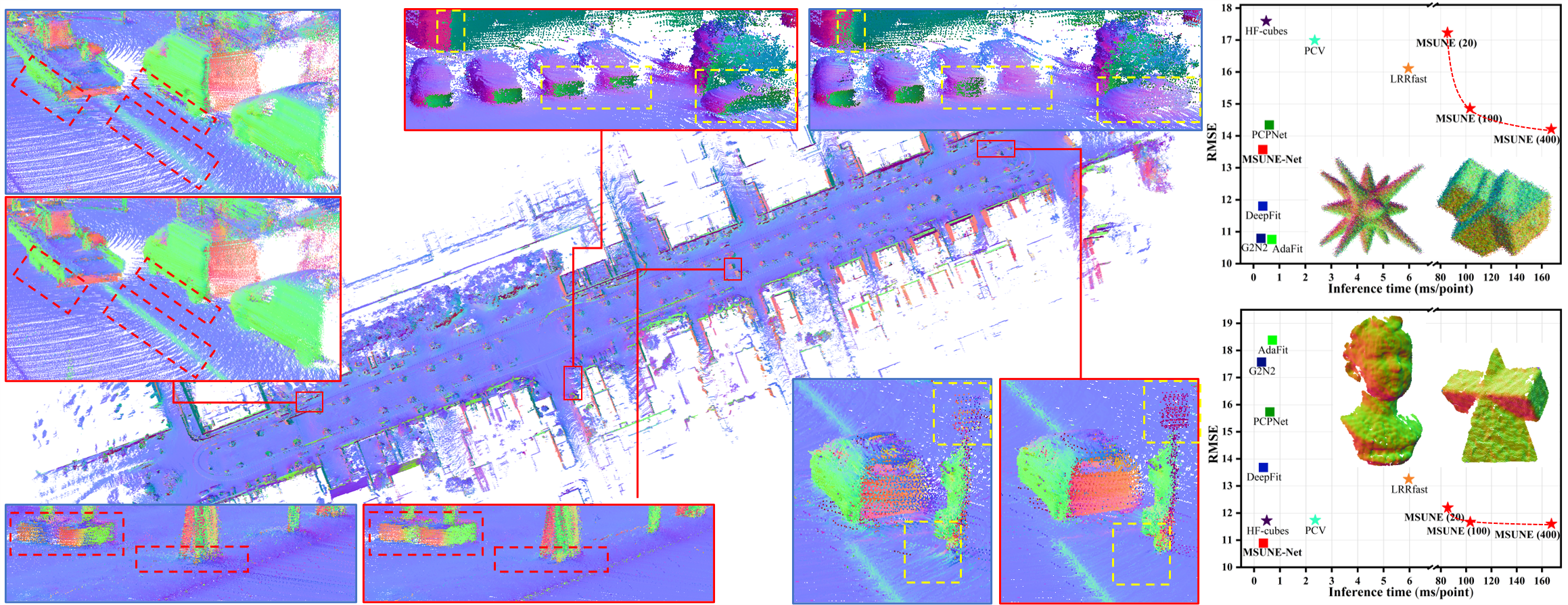
Figure 1: MSUNE-Net shows higher performance than conventional methods and supervised deep normal estimators on the LiDAR point clouds (Left), sequence 06 of KITTI [2], and the Kinect dataset proposed in [1] (Bottom right). It is even superior to some supervised deep learning methods on the synthesized dataset of PCPNet [3] (Top right). MSUNE also outperforms previous methods in RMS errors on the Kinect dataset, when 400 initial candidate normals are employed. Some estimated normals for LiDAR point cloud by DeepFit [4] and MSUNE-Net are zoomed in blue and red boxes respectively. Compared with Deepfit, sharp features and tiny structures are better preserved in MSUNE-Net. Meanwhile, scanner noises are well suppressed by MSUNE-Net. Colors encode the orientation of the normals.

Point clouds have emerged as a fundamental representation in reverse engineering, indoor scene modeling, robot grasping, and autonomous driving. Their surface normals, defining the local structure of the underlying surface to the first order, play a major role in these applications. Many deep neural networks have been proposed for more accurate normal estimation [5, 4, 6, 7, 8, 3, 9, 10], and they surpass the conventional methods [1, 11, 12, 13, 14, 12] indeed. But their performance drops significantly on raw point clouds since they are trained on synthesized datasets [4, 6] only, and the unseen target domains have considerable distribution shifts. An illustration can be seen in Fig. 1 where the point clouds of LiDAR, Kinect, and synthetic datasets show three different characteristics. It is a challenge to annotate point-wise normal precisely for the noisy data from various scanners, which makes them inaccessible to supervised learning that requires massive pairs of point positions and normals. Consequently, it is more desirable to estimate accurate normals for raw point clouds scanned by common sensors, such as Kinect and LiDAR, without resorting to normal annotations, as shown in Fig. 1.

Conventional normal estimators [15, 11, 1, 14, 16] are unsupervised. But they tend to over smooth the inputs or may introduce additional artifacts around salient features. Manually tuning of an algorithm’s parameters is necessary to accommodate different noise levels and feature scales of various point clouds. Recent developments on unsupervised image denoising [17, 18] and point cloud denoising [19, 20] have demonstrated the potential of learning from multiple random sampled observations, whether it be a pixel or a point, rather than relying on ground truth labels. It also sheds light on our scenario, even though the problem is different. We are attempting to estimate the properties of noisy observations while they are working on denoising the observations. More importantly, we have to address the multimodal distribution of randomly sampled candidate normals to achieve feature-preserving normal estimation. This is a departure from the unimodal distribution assumed in [17, 18]. [19, 20] resort to the point cloud appearance to transform the distribution into a single mode, assuming the appearance is credible. Instead, we hope to solve the problem directly from observed point positions and do not depend on further input sources and assumptions. Hence the scenario of unsupervised normal estimation of noisy 3D point clouds is more challenging, which presents both theoretical difficulties and practical obstacles. At present, there is no literature addressing the problem of unsupervised normal estimation based on neural networks, to our knowledge.

This paper proves that the ground truth normal of a query point is the expectation of a set of randomly sampled candidate normals, provided that the underlying surface is smooth and noise has zero mean. However, these assumptions may be invalid for scanned points with sharp features. Hence, we propose a practical unsupervised normal estimation paradigm driven by multi-sample consensus and two of its implementations: an optimization-based method (MSUNE), and a deep learning-based one (MSUNE-Net). The paradigm may be also applicable to other unsupervised low-level image and point cloud processing. Section 7 reports its preliminary application to improve DMR [20], a SOTA unsupervised point cloud denoising network.

The paradigm consists of three stages: multi-candidate sampling, candidate rejection, and mode determination. The latter two are driven by neighbor point consensus and candidate consensus respectively. These stages are easier to understand with a brief introduction to MSUNE, as it is a typical implementation of the paradigm. MSUNE estimates one normal for each query point from a surface patch, i.e. a neighborhood, centered on the point.

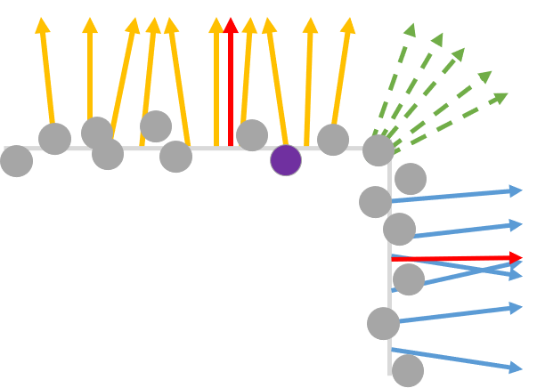
Figure 2: A 2D illustration of candidate normal distribution of a point close to a sharp edge.

Taking a query point near some sharp edge, the purple point in Fig. 2, as an example, MSUNE generates multiple initial candidate normals (orange, blue, and green normals) randomly from its neighborhood. Then a more feasible set of candidate normals is built by rejecting some blurry candidates (green dotted normals) that do not conform to the underlying geometry structure. These normals have low consensus measured by the neighbor points, i.e.  they are supported by fewer neighbor points. The distribution of the feasible candidates (orange and blue solid normals) is still a multimodal distribution. There are two modes in the 2D illustration, i.e.  the coarse and thin red normals. Consequently, a robust candidate consensus loss function is designed in the third stage to locate the main mode (the coarse red normal), which is a feature-preserving normal with the greatest consensus of the feasible candidates. By minimizing the loss, MSUNE outputs a high-quality approximation of the ground truth normal. Higher accuracy can be achieved by sampling more initial candidate normals as shown in Fig. 1. It outperforms SOTA conventional normal estimators and supervised deep learning methods on real scan data when 400 candidates are sampled. While it is time-consuming even when 20 candidates per query point are used since the optimization is also slow.

MSUNE-Net further introduces a patch-based neural network, which explores the non-local patch self-similarity of point clouds to boost multi-sample consensus. Compared with MSUNE, learning a normal solely on multiple candidates from the query point’s neighborhood, MSUNE-Net can also learn from other query points with similar patches, which means the candidate consensus loss is defined on much more candidates implicitly even if the network is trained with far fewer candidates per query point. Consequently, a better approximation of the main mode of the candidates is calculated. It is also 100 times more efficient since there is only a network forward pass in inferencing. The manipulation and optimization in the three stages only occur during training. As illustrated in Fig. 1 and supported by the comprehensive experiments, our unsupervised approaches outperform the conventional methods and the cutting-edge deep learning-based methods on real Kinect [1, 21] and LiDAR datasets [2]. It is also noteworthy that the unsupervised MSUNE-Net surpasses some supervised deep normal estimators, such as HoughCNN and PCPNet, on the most common synthetic dataset.

To summarize, our main contributions are three-fold:

• A multi-sample consensus paradigm for unsupervised normal estimation, consisting of candidate sampling, candidate rejection, and mode determination, is proposed. It is also applicable to other low-level image and point cloud processing, such as unsupervised deep point cloud denoising.

• MSUNE, a robust optimization method driven by the multi-sample consensus, is proposed. It outperforms all the SOTA optimization-based and supervised deep learning based normal estimators on real scanned point clouds. It is even superior to some supervised deep normal estimators on the most common synthesized dataset.

• MSUNE-Net, an unsupervised deep learning method boosting the multi-sample consensus, is proposed. It is more accurate than MSUNE and is 100 times faster.

2 Related work

Normal estimation. Normal estimation of point clouds is a long-standing problem in geometry processing, mainly because it is directly used in many downstream tasks. The most popular and simplest method for normal estimation is based on Principal Component Analysis (PCA) [11], which is utilized to find the eigenvectors of the covariance matrix constructed by neighbor points. Following this work, many variants have been proposed [22, 23, 24]. There are also methods based on Voronoi cells [25, 26, 27, 28]. But none of them are designed to handle outliers or sharp features [13]. Sparse representation methods [12, 16, 29] and robust statistical techniques [13, 30, 31, 32, 33, 34] are employed to improve normal estimation for point clouds with sharp features. And some other methods, such as Hough Transform [14], also show impressive results. Although these algorithms are unsupervised and have strong theoretical guarantees, they are very sensitive to noise. In addition, advanced conventional estimation methods are usually much slower than deep normal estimators, since the latter infers normals only with a forward propagation.

In recent years, with the wide application and success of deep learning, normal estimation methods based on deep learning have also been proposed. There have been some attempts [35, 36, 7] to project local unstructured points into a regular domain for direct application of CNN architectures. With the advent of geometric deep learning, PointNet [3, 37, 38] and graph neural networks [39] are employed to learn a direct mapping from raw points to ground truth normals. More recent works have attempted to embed conventional methods into deep learning [40, 9, 41]. Ben et al. [4] (DeepFit) append weighted least squares polynomial surface fitting module to a PointNet network for point-wise weights estimation in an end-to-end manner. Zhu et al. [6] (AdaFit) add an additional offset prediction to improve the quality of the estimated normals. Zhang et al. [8] propose a geometry-guided neural network (G2N2) for robust and detail-preserving normal estimation. However, the above approaches are supervised, as they require a ground truth normal for each point. The ground truth normals are produced by sampling points from synthetic meshes or surfaces. Their results on the real scan data are unsatisfactory. Our approach does not require ground truth normals and performs well for real scan data.

Unsupervised learning. Unsupervised deep learning has been intensively studied by researchers in recent years with the aim of alleviating the time-consuming and laborious data annotation challenge. When training a network, it needs some reasonable constraints to replace the ground truth. For advanced semantic tasks, pseudo-labeling [42, 43, 44] is a common idea. The pseudo labels may be from other pre-trained models or the network being trained with proper weight initialization from other supervised networks or pretext tasks. In our methods, the pseudo labels are generated from unlabeled data directly without relying on other methods. Moreover, different from these methods which depend on one accurate pseudo-label per-point, we randomly generate multiple low-cost and low-quality pseudo labels, i.e. multi-candidate normals, for each point.

Low-level tasks, such as image denoising and point cloud denoising, usually operate under the assumption that noisy observations are stochastic realizations distributed around clean values. Lehtinen et al. [17] utilize multiple noisy observations from image pairs to denoise an image. Going one step further, Noise2Void [45] and Noise2Self [18] remove the requirement of paired noise corruptions and instead work on a single image. Hermosilla et al. [19] extend unsupervised image denoisers to 3D point clouds by introducing a proximity-appearance prior. The prior actually restricts the distribution of the candidate positions to have a single modal. Based on the core idea of [19], Luo et al.  [20] present an autoencoder-like neural network to improve the accuracy of denoising. Unfortunately, they cannot be naively extended to normal estimation, since they denoise the noisy observations but we estimate the indirect geometry property of the noisy observations. They take an approximated expectation of multiple random samples as the denoised pixel or point. While we locate the main mode of candidate normals without aid from other properties. The proposed MSUNE-Net is the first unsupervised deep normal estimator as far as we know.

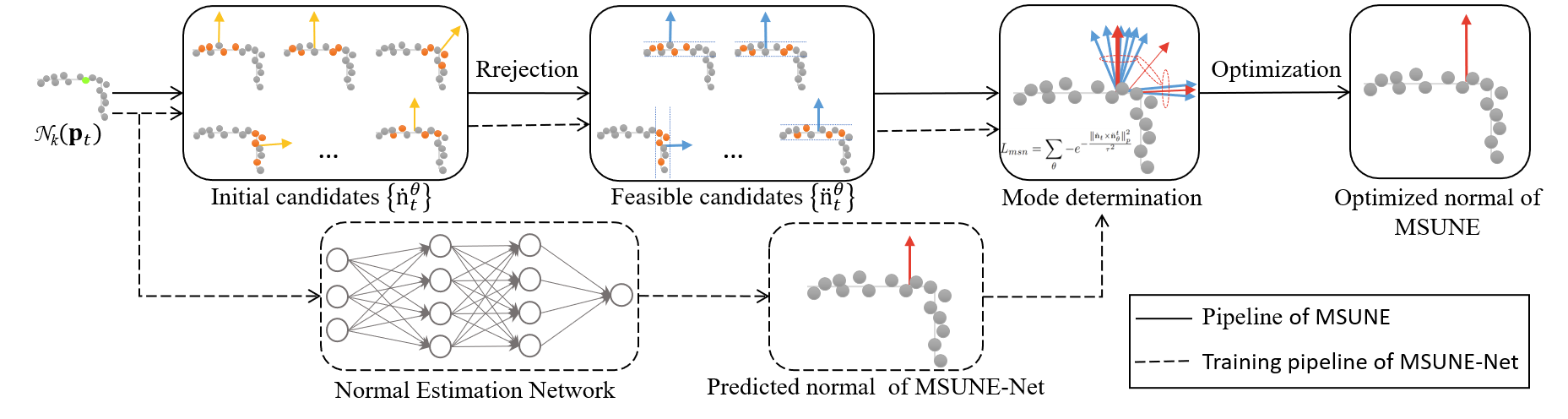
Figure 3: The proposed framework for unsupervised normal estimation. To estimate a normal for the query point $\mathbf{p}_{t}$, MSUNE initializes a set of candidate normals first. It then rejects some unconvincing normals to build feasible candidates $\{\ddot{\mathbf{n}}^{t}_{\theta}\}$. At last, it learns a noise-free normal of $\mathbf{p}_{t}$ by minimizing the proposed candidate consensus loss defined by the feasible candidates. Instead of learning a normal just from the neighborhood of the point, MSUNE-Net can be defined by appending a normal estimation network to MSUNE. Consequently, MSUNE-Net learns more creditable normals from massive data in an unsupervised way.

3 The Multi-sample Consensus Paradigm

We propose a practical unsupervised normal estimation paradigm driven by multi-sample consensus. For each query point of a point cloud, the paradigm predicts the normal of the point from a neighborhood centered on the point. It consists of three stages: multi-candidate sampling, candidate rejection, and mode determination. The first one is for sampling enough candidates, which may be from a multimodal distribution, from the point’s neighborhood. The latter two stages are designed to approximate the main mode of those candidates. The candidate rejection stage filters out some candidates with lower consensus from neighbor points, and the mode determination stage estimates the main mode of the rest feasible candidates. The paradigm is actually general enough to be applied to other unsupervised low-level image and point cloud processing. A point cloud denoising example is reported in Section 7. Two implementations of the paradigm for normal estimation: an optimization-based method (MSUNE), and a deep learning-based one (MSUNE-Net), will be introduced in the next two sections.

4 MSUNE

Given a 3D point cloud $P=\{\mathbf{p}_{t}~{}|~{}t=1,2,\cdots,N\}$ and a query point $\mathbf{p}_{t}$, MSUNE takes the $k$ nearest neighbors of it, $\mathcal{N}_{k}(\mathbf{p}_{t})\subset P$, as input and predicts a normal $\hat{\mathbf{n}}_{t}$ for the point. MSUNE’s pipeline is presented in Fig. 3. Multiple candidate normals can be initialized by a set of randomly sampled points from its neighborhood, which is detailed in subsection 4.1. We prove that the correct normal can be approximated by minimizing Eq. 2 when the underlying surface is smooth.

However, if $\mathbf{p}_{t}$ lies near some sharp features, The underlying surface of its neighborhood actually consists of multiple piecewise smooth surfaces and the candidate normals are sampled from a multimodal distribution, which invalidates the conclusion. As illustrated in Fig. 2, the randomly initialized candidates also include some disturbing normals in blue which are associated with the plane on the opposite side of the edge, and some blurry normals in green if the sampled points across the edge. Robust statistical techniques are used to filter out the impact of these undesired candidate normals driven by multi-sample consensus. The blurry normals can be rejected by the consensus of $\mathbf{p}_{t}^{\prime}s$ neighbor points, i.e. there are a few neighbor points supporting a plane with a blurry normal (subsection 4.2). For the rest candidates, instead of approximating their expected value by minimizing the square of the Euclidean distance between $\hat{\mathbf{n}}_{t}$ and the candidates, we design a novel candidate consensus loss (subsection 4.3). The disturbing modes have fewer supporters in the candidate normals. The main mode of the candidate normals owns the greatest consensus of them, which can be approximated by minimizing the loss function.

4.1 Multi-candidate sampling

The initial candidate normals $\dot{N}_{t}=\{\dot{\mathbf{n}}^{t}_{\theta}\}$ of the query point are built from its adaptive neighborhood $\mathcal{N}_{\hat{k}}(\mathbf{p}_{t})$ of size $\hat{k}$. $\dot{\mathbf{n}}^{t}_{\theta}$ is the normal of a plane $\theta$ determined by $k_{s}$ points which are randomly selected from $\mathcal{N}_{\hat{k}}(\mathbf{p}_{t})$, and a typical setting is $k_{s}=3$. Thus it is efficient to build a large set of candidates for each query point. It is proven in the following subsection that the noise-free normal $\mathbf{n}_{t}$ is the expectation of $\dot{\mathbf{n}}^{t}_{\theta}$ if the underlying surface of the noisy point cloud is smooth and the expectation of the noise is zero. Hence a faithful approximation can be achieved if $\dot{N}_{t}$ includes sufficient candidates.

4.1.1 Theoretical analysis

Let $\tilde{\mathbf{p}}_{t}$ be a point on the underlying smooth surface $S$ of the point cloud, and its noisy observation is $\mathbf{p}_{t}=\tilde{\mathbf{p}}_{t}+\mathbf{\varepsilon}_{t}$. $U$ is an open set on $S$ centering at $\tilde{\mathbf{p}}_{t}$. The normal of it is denoted as $\mathbf{n}_{t}$. For any three non collinear points $\{\tilde{\mathbf{p}}^{t}_{\theta 1},\tilde{\mathbf{p}}^{t}_{\theta 2},\tilde{\mathbf{p}}^{t}_{\theta 3}\}$ on U, $\tilde{\mathbf{n}}^{t}_{\theta}=\left(\tilde{\mathbf{p}}^{t}_{\theta 2}-\tilde{\mathbf{p}}^{t}_{\theta 1}\right)\times\left(\tilde{\mathbf{p}}^{t}_{\theta 3}-\tilde{\mathbf{p}}^{t}_{\theta 1}\right)$ is the vector corresponding to the plane $\theta$ spanned by $\{\tilde{\mathbf{p}}^{t}_{\theta 1},\tilde{\mathbf{p}}^{t}_{\theta 2},\tilde{\mathbf{p}}^{t}_{\theta 3}\}$. Their noisy observations are $\left\{\mathbf{p}^{t}_{\theta 1},\mathbf{p}^{t}_{\theta 2},\mathbf{p}^{t}_{\theta 3}\right\}$, where $\mathbf{p}^{t}_{\theta j}=\tilde{\mathbf{p}}^{t}_{\theta j}+\mathbf{\varepsilon}_{j},j=1,2,3$. Each group of them defines an candidate normal $\dot{\mathbf{n}}^{t}_{\theta}$. Here, $\{\tilde{\mathbf{p}}^{t}_{\theta 1},\tilde{\mathbf{p}}^{t}_{\theta 2},\tilde{\mathbf{p}}^{t}_{\theta 3}\}$ are sorted counterclockwise and noise $\mathbf{\varepsilon}_{j}=(\varepsilon_{xj},\varepsilon_{yj},\varepsilon_{zj})^{T}$ is assumed to be independent for components. For convenience, we do not normalize $\tilde{\mathbf{n}}^{t}_{\theta}$ and $\dot{\mathbf{n}}^{t}_{\theta}$ in the following theoretical analysis. We have the following theorem.

Theorem 1.

If $E\{\varepsilon\}=0$, then we have $E\left\{\dot{\mathbf{n}}^{t}_{\theta}\right\}=E\left\{\tilde{\mathbf{n}}^{t}_{\theta}\right\}$.

Proof.

Since $\mathbf{p}^{t}_{\theta j}=\tilde{\mathbf{p}}^{t}_{\theta j}+\mathbf{\varepsilon}_{j},j=1,2,3$, we have

$$\begin{array}[]{l}\mathbf{p}^{t}_{\theta 1}=\left(\tilde{x}_{\theta 1}+\varepsilon_{x_{\theta 1}},\tilde{y}_{\theta 1}+\varepsilon_{y_{\theta 1}},\tilde{z}_{\theta 1}+\varepsilon_{z_{\theta 1}}\right)^{T},\\ \mathbf{p}^{t}_{\theta 2}=\left(\tilde{x}_{\theta 2}+\varepsilon_{x_{\theta 2}},\tilde{y}_{\theta 2}+\varepsilon_{y_{\theta 2}},\tilde{z}_{\theta 1}+\varepsilon_{z_{\theta 1}}\right)^{T},\\ \mathbf{p}^{t}_{\theta 3}=\left(\tilde{x}_{\theta 3}+\varepsilon_{x_{\theta 3}},\tilde{y}_{\theta 3}+\varepsilon_{y_{\theta 3}},\tilde{z}_{\theta 3}+\varepsilon_{z_{\theta 3}}\right)^{T},\\ \end{array}$$

where $\tilde{\mathbf{p}}^{t}_{\theta j}=\left(\tilde{x}_{\theta j},\tilde{y}_{\theta j},\tilde{z}_{\theta j}\right)^{T}$ for $j=1,2,3$ and $\varepsilon_{*_{\theta i}}$ is independent for $*=x,y,z$ and $i=1,2,3$. Then, we have

$$\begin{array}[]{l}\dot{\mathbf{n}}^{t}_{\theta}=\left(\mathbf{p}^{t}_{\theta 2}-\mathbf{p}^{t}_{\theta 1}\right)\times\left(\mathbf{p}^{t}_{\theta 3}-\mathbf{p}^{t}_{\theta 1}\right)\\ =\left(\begin{array}[]{c}\tilde{x}_{\theta 2}-\tilde{x}_{\theta 1}+\varepsilon_{x_{\theta 2}}-\varepsilon_{x_{\theta 1}}\\ \tilde{y}_{\theta 2}-\tilde{y}_{\theta 1}+\varepsilon_{y_{\theta 2}}-\varepsilon_{y_{\theta 1}}\\ \tilde{z}_{\theta 2}-\tilde{z}_{\theta 1}+\varepsilon_{z_{\theta 2}}-\varepsilon_{z_{\theta 1}}\\ \end{array}\right)\times\\ ~{}~{}~{}\left(\begin{array}[]{c}\tilde{x}_{\theta 3}-\tilde{x}_{\theta 1}+\varepsilon_{x_{\theta 3}}-\varepsilon_{x_{\theta 1}}\\ \tilde{y}_{\theta 3}-\tilde{y}_{\theta 1}+\varepsilon_{y_{\theta 3}}-\varepsilon_{y_{\theta 1}}\\ \tilde{z}_{\theta 3}-\tilde{z}_{\theta 1}+\varepsilon_{z_{\theta 3}}-\varepsilon_{z_{\theta 1}}\\ \end{array}\right).\\ \end{array}$$

Denote the first component of $\dot{\mathbf{n}}^{t}_{\theta}$ as $\dot{\mathbf{n}}^{t}_{\theta,x}$. According to the definition of cross product, we have

$$\begin{array}[]{l}\dot{\mathbf{n}}^{t}_{\theta,x}=\left(\tilde{y}_{\theta 2}-\tilde{y}_{\theta 1}+\varepsilon_{y_{\theta 2}}-\varepsilon_{y_{\theta 1}}\right)\left(\tilde{z}_{\theta 3}-\tilde{z}_{\theta 1}+\varepsilon_{z_{\theta 3}}-\varepsilon_{z_{\theta 1}}\right)-\\ \left(\tilde{y}_{\theta 3}-\tilde{y}_{\theta 1}+\varepsilon_{y_{\theta 3}}-\varepsilon_{y_{\theta 1}}\right)\left(\tilde{z}_{\theta 2}-\tilde{z}_{\theta 1}+\varepsilon_{z_{\theta 2}}-\varepsilon_{z_{\theta 1}}\right)\\ =\left(\tilde{y}_{\theta 2}-\tilde{y}_{\theta 1}\right)\left(\tilde{z}_{\theta 3}-\tilde{z}_{\theta 1}\right)+\left(\tilde{y}_{\theta 2}-\tilde{y}_{\theta 1}\right)\left(\varepsilon_{z_{\theta 3}}-\varepsilon_{z_{\theta 1}}\right)\\ +\left(\tilde{z}_{\theta 3}-\tilde{z}_{\theta 1}\right)\left(\varepsilon_{y_{\theta 2}}-\varepsilon_{y_{\theta 1}}\right)+\left(\varepsilon_{y_{\theta 2}}-\varepsilon_{y_{\theta 1}}\right)\left(\varepsilon_{z_{\theta 3}}-\varepsilon_{z_{\theta 1}}\right)\\ -\left(\tilde{y}_{\theta 3}-\tilde{y}_{\theta 1}\right)\left(\tilde{z}_{\theta 2}-\tilde{z}_{\theta 1}\right)-\left(\tilde{y}_{\theta 3}-\tilde{y}_{\theta 1}\right)\left(\varepsilon_{z_{\theta 2}}-\varepsilon_{z_{\theta 1}}\right)\\ -\left(\tilde{z}_{\theta 2}-\tilde{z}_{\theta 1}\right)\left(\varepsilon_{y_{\theta 3}}-\varepsilon_{y_{\theta 1}}\right)-\left(\varepsilon_{y_{\theta 3}}-\varepsilon_{y_{\theta 1}}\right)\left(\varepsilon_{z_{\theta 2}}-\varepsilon_{z_{\theta 1}}\right)\\ \end{array}$$

Then,

$$\begin{array}[]{l}E\{\dot{\mathbf{n}}^{t}_{\theta,x}\}=E_{\{\varepsilon,\tilde{\mathbf{p}}^{t}_{\theta 1},\tilde{\mathbf{p}}^{t}_{\theta 2},\tilde{\mathbf{p}}^{t}_{\theta 3}\}}\{\dot{\mathbf{n}}^{t}_{\theta,x}\}\\ ~{}~{}~{}~{}~{}~{}~{}~{}~{}~{}~{}=E_{\{\tilde{\mathbf{p}}^{t}_{\theta 1},\tilde{\mathbf{p}}^{t}_{\theta 2},\tilde{\mathbf{p}}^{t}_{\theta 3}\}}\{E_{\{\varepsilon\mid\tilde{\mathbf{p}}^{t}_{\theta 1},\tilde{\mathbf{p}}^{t}_{\theta 2},\tilde{\mathbf{p}}^{t}_{\theta 3}\}}\{\dot{\mathbf{n}}^{t}_{\theta,x}\}\}\\ ~{}~{}~{}~{}~{}~{}~{}~{}~{}~{}~{}=E_{\{\tilde{\mathbf{p}}^{t}_{\theta 1},\tilde{\mathbf{p}}^{t}_{\theta 2},\tilde{\mathbf{p}}^{t}_{\theta 3}\}}\{\left(\tilde{y}_{\theta 2}-\tilde{y}_{\theta 1}\right)\left(\tilde{z}_{\theta 3}-\tilde{z}_{\theta 1}\right)\\ ~{}~{}~{}~{}~{}~{}~{}~{}~{}~{}~{}~{}~{}~{}~{}~{}~{}~{}~{}~{}~{}~{}~{}~{}~{}~{}~{}~{}~{}~{}-\left(\tilde{y}_{\theta 3}-\tilde{y}_{\theta 1}\right)\left(\tilde{z}_{\theta 2}-\tilde{z}_{\theta 1}\right)\}\\ ~{}~{}~{}~{}~{}~{}~{}~{}~{}~{}~{}=E_{\{\tilde{\mathbf{p}}^{t}_{\theta 1},\tilde{\mathbf{p}}^{t}_{\theta 2},\tilde{\mathbf{p}}^{t}_{\theta 3}\}}\{\tilde{\mathbf{n}}^{t}_{\theta,x}\}\\ ~{}~{}~{}~{}~{}~{}~{}~{}~{}~{}~{}=E\{\tilde{\mathbf{n}}^{t}_{\theta,x}\},\\ \end{array}$$

where, $\tilde{\mathbf{n}}^{t}_{\theta,x}$ represents the first component of $\tilde{\mathbf{n}}^{t}_{\theta}$. Therefore,

$$\begin{array}[]{l}E\{\dot{\mathbf{n}}^{t}_{\theta}\}=E_{\{\varepsilon,\tilde{\mathbf{p}}^{t}_{\theta 1},\tilde{\mathbf{p}}^{t}_{\theta 2},\tilde{\mathbf{p}}^{t}_{\theta 3}\}}\{\dot{\mathbf{n}}^{t}_{\theta}\}\\ ~{}~{}~{}~{}~{}~{}~{}~{}~{}=E_{\{\tilde{\mathbf{p}}^{t}_{\theta 1},\tilde{\mathbf{p}}^{t}_{\theta 2},\tilde{\mathbf{p}}^{t}_{\theta 3}\}}\{\tilde{\mathbf{n}}^{t}_{\theta}\}=E\{\tilde{\mathbf{n}}^{t}_{\theta}\}.\\ \end{array}$$

∎

Corollary 1.

If $S$ is smooth and $E\{\varepsilon\}=0$, then $E\{\dot{\mathbf{n}}^{t}_{\theta}\}$ is on the same line with $\mathbf{n}_{t}$.

Proof.

Since $S$ is smooth, a small enough neighborhood $U$ can be regarded as a plane. Then, for any three non collinear points $\{\tilde{\mathbf{p}}^{t}_{\theta 1},\tilde{\mathbf{p}}^{t}_{\theta 2},\tilde{\mathbf{p}}^{t}_{\theta 3}\}$, $\tilde{\mathbf{n}}^{t}_{\theta}=k_{\theta}\mathbf{n}_{t}$, where $k_{\theta}$ is a coefficient related to $\{\tilde{\mathbf{p}}^{t}_{\theta 1},\tilde{\mathbf{p}}^{t}_{\theta 2},\tilde{\mathbf{p}}^{t}_{\theta 3}\}$. Thus, $E\left\{\tilde{\mathbf{n}}^{t}_{\theta}\right\}=k\mathbf{n}_{t}$, where $k=E\{k_{\theta}\}$. Then we have $E\left\{\dot{\mathbf{n}}^{t}_{\theta}\right\}=k\mathbf{n}_{t}$ for $E\{\varepsilon\}=0$. Since $\{\tilde{\mathbf{p}}^{t}_{\theta 1},\tilde{\mathbf{p}}^{t}_{\theta 2},\tilde{\mathbf{p}}^{t}_{\theta 3}\}$ are sorted counterclockwise, $k_{\theta}$ is positive. Therefore $k\neq 0$. The conclusion is proofed. ∎

The minimum of the following optimization problem

$$\underset{\mathbf{z}}{\operatorname{argmin}}E_{\dot{\mathbf{n}}^{t}_{\theta}}\left\{\|\mathbf{z}-\dot{\mathbf{n}}^{t}_{\theta}\|_{F}^{2}\right\},$$ (1)

is found at the expectation of $\dot{\mathbf{n}}^{t}_{\theta}$, i.e. $\mathbf{z}=E\{\dot{\mathbf{n}}^{t}_{\theta}\}$. We have proven that $E\{\dot{\mathbf{n}}^{t}_{\theta}\}=k\mathbf{n}_{t}$. Therefore, given finite candidate normals $\dot{N}_{t}$, we can approximate the direction of $\mathbf{n}_{t}$ by the following optimization problem

$$\underset{\mathbf{z}}{\operatorname{argmin}}\sum_{\dot{\mathbf{n}}^{t}_{\theta}\in\dot{N}_{t}}\left\{\|\mathbf{z}-\dot{\mathbf{n}}^{t}_{\theta}\|_{F}^{2}\right\},$$ (2)

when the surface is smooth. In the implementation, the candidate normals $\dot{\mathbf{n}}^{t}_{\theta}$ are normalized. To avoid introducing unnecessary symbols, we still use $\dot{\mathbf{n}}^{t}_{\theta}$ to represent the normalized vector in the following discussion. It is noteworthy that the larger the size of the candidate set $\dot{N}_{t}$, the better the approximation.

4.1.2 Adaptive neighborhood

In theoretical analysis, the neighborhood $\mathcal{N}_{\hat{k}}(\mathbf{p}_{t})$ should be as small as possible to be regarded as a plane. But, a small neighborhood is inadequate to depict the underlying structure of the surface when the point cloud is polluted by large noise. Therefore, the neighborhood size is adaptively determined. Specifically, for each point $\mathbf{p}_{t}$, we first apply the local covariance analysis to characterize its noise level $f_{t}$ (Section 4 in [1]). The average $f=\sum_{t=1}^{N}f_{t}/N$ is then utilized to describe the noise scale of the whole point cloud. Finally, a suitable neighborhood size is determined according to the interval in which $f$ is located: $\hat{k}=k_{i},if~{}l_{i-1}\leq f<l_{i}$. We take $k_{1}=32$, $k_{2}=128$, $k_{3}=256$, $k_{4}=450$, $l_{0}=0$, $l_{1}=0.02$, $l_{2}=0.14$, and $l_{3}=0.16$, $l_{4}=0.3$ in our experiments.

4.2 Candidates rejection

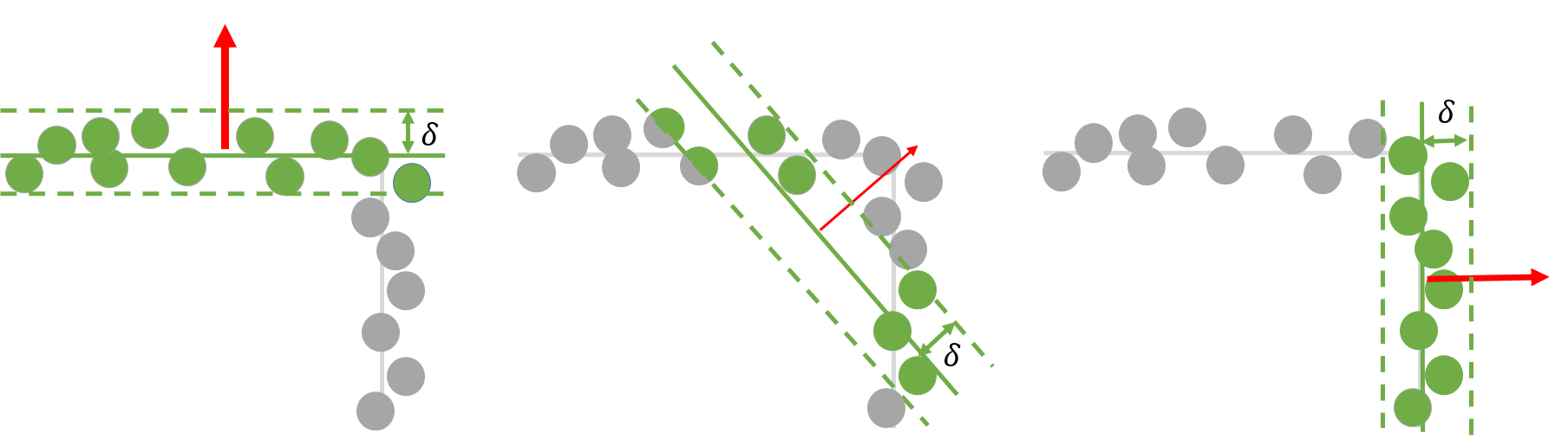
Figure 4: We are eager to find normals corresponding to planes with more inlier points (green points). The thickness of the normal is determined by the number of inlier points.

The randomly initialized candidates are noisy unavoidably, and their number may be limited in practice. Hence it is necessary to reject some infeasible normals for a high-quality approximation of Eq. 2. Here we follow the idea of kernel density estimation. For each candidate normal $\dot{\mathbf{n}}^{t}_{\theta}$, we define a score $s^{t}_{\theta}$ based on the distances of all neighbor points to its corresponding plane $\theta$:

$$s^{t}_{\theta}=\sum_{i=1}^{\hat{k}}e^{-\frac{\left(d(\mathbf{p}_{t}^{i},\theta)\right)^{2}}{\sigma^{2}}},$$ (3)

where $\mathbf{p}_{t}^{i}\in\mathcal{N}_{\hat{k}}(p_{t})$ is a neighbor point of $\mathbf{p}_{t}$, $d(\mathbf{p}_{t}^{i},\theta)$ represents the Euclidean distance from point $\mathbf{p}_{t}^{i}$ to the plane $\theta$, and $\sigma$ is the bandwidth of the Gaussian kernel function. A higher score means a higher consensus reached by the query point’s neighbor points. It is designed to reject normals supported by fewer inliers, as shown in Fig. 4. When $d(\mathbf{p}_{t}^{i},\theta)$ is less than the bandwidth $\sigma$, the point $\mathbf{p}_{t}^{i}$ is regarded as an inlier point of the plane $\theta$. It will give $\theta$ a strong support $e^{-\left(d(\mathbf{p}_{t}^{i},\theta)\right)^{2}/\sigma^{2}}$. The larger $s^{t}_{\theta}$ is, the more feasible the normal is. Therefore we sort the initialized candidate normals according to the scores, and delete 20% of those that get lower scores. The remaining normals are feasible candidate normals, denoted by $\ddot{N}_{t}=\{\ddot{\mathbf{n}}^{t}_{\theta}\}$.

The value of $\sigma$ should depend on the noise level of the point cloud. It seems that $\sigma$ should take a large value for point clouds with large noise since a high noise level will result in more neighbor points with large $d(\mathbf{p}_{t}^{i},\theta)$ even the plane is feasible. Conversely, when the noise of the point cloud is small, $\sigma$ should take a smaller value. But in the experiments, we find that a large $\sigma$ does not work well for either large or small noise. Therefore, we only employ this rejection strategy for noise-free or small noise point clouds whose average noise level $f$ located in the first two intervals, as stated in Section 4.1.2. They usually require a small $\sigma$. In our implementation, we set it as one percent of the neighborhood radius.

4.3 Mode determination

Previous unsupervised denoisers all pursue a clean position as the average of all the candidates. But the distribution of the feasible candidate normals of a point close to sharp features is still a multimodal distribution, as demonstrated in Fig. 2. It should be possible to exclude the interference of disturbing normals and select the main mode, since $\mathbf{p}_{t}$ is not exactly on the edge. There may be also some other causes since the limited candidates are randomly determined from the noisy point cloud and our candidate rejection strategy is naive. Anyway, the average of all the feasible candidates is still far from expected. Inspired by the idea of robust statistical techniques, we design the following candidate consensus loss function for normal estimation:

$$L_{{\color[rgb]{0,0,0}ccn}}=\sum_{\theta}-e^{-\frac{\left\|\hat{\mathbf{n}}_{t}\times\ddot{\mathbf{n}}^{t}_{\theta}\right\|_{F}^{2}}{\tau^{2}}},~{}~{}~{}\ddot{\mathbf{n}}^{t}_{\theta}\in\ddot{N}_{t},$$ (4)

where $\hat{\mathbf{n}}_{t}$ is the predicted normal, $\tau=\sin\alpha$ denotes the bandwidth of the Gaussian kernel function. $\alpha=\frac{\pi}{6}$ in all the experiments.

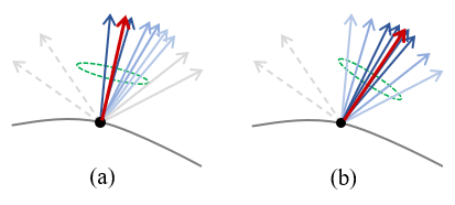
Figure 5: Candidate consensus loss function can effectively exclude the influence of disturbing normals (dotted normals). The red normals in (a) and (b) are the average normals of all candidates and solid candidates, respectively. The candidates in the green circles are regarded as inliers of the red normals. The darker the color, the higher their contribution to the red normals, which are determined by the candidate consensus loss.

When the angle between the predicted normal and the candidate normal is less than $\alpha$, we consider this candidate to be an inlier of the predicted normal. Thus a predicted normal with the most inliers, i.e. with the greatest consensus of the candidate normals, is desired. As shown in Fig. 5, this mechanism can effectively overcome the influence of disturbing normals.

5 MSUNE-Net

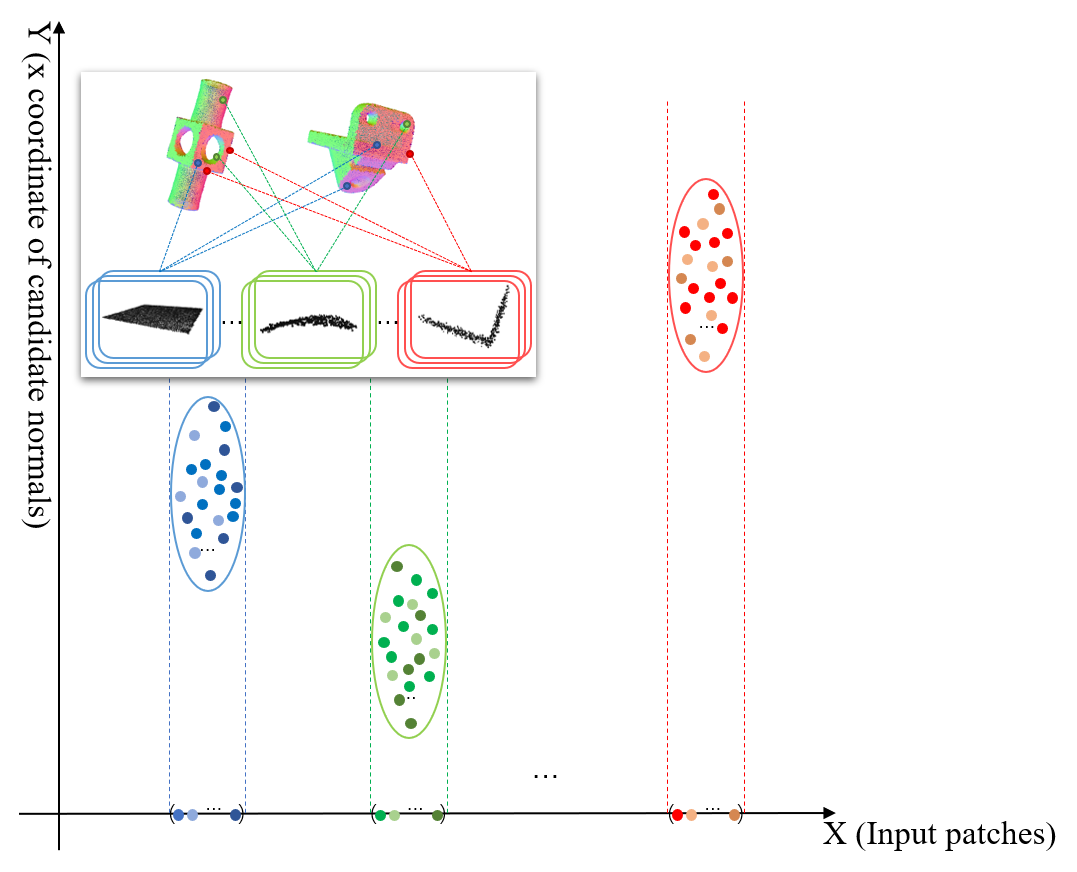
Figure 6: More candidate normals from similar patches contribute the normal approximation of the current query point implicitly when a patch-based network is employed. For simplicity, the input patches and candidate normals are drawn as points.

MSUNE outperforms previous conventional methods and is comparable with some supervised deep normal estimators, such as PCPNet (see Section 6 for details). But it needs to calculate a large number of candidate normals and solve an optimization problem at each point. They are both time-consuming. Therefore, we wish to develop an unsupervised deep learning method. All the time-consuming operations will be transferred to the training process and only a network forward pass is necessary for normal inference. It is noteworthy that the network is not just an accelerator that learns from the single output normal of MSUNE, but is trained on a dataset with the candidate consensus loss defined by feasible candidates. Consequently, MSUNE-Net is also superior to MSUNE in performance. The reason is explained in the following subsection.

5.1 Patch-based network

Patch-based learning is the most common approach adopted by existing deep normal estimators [3, 4, 8]. They take the patch centered at each query point as the input and the patch is normalized in preprocessing to remove unnecessary degrees of freedom from scale and rotation. We find that the patch self-similarity across point clouds is explored by such networks, and a patch-based network is a perfect fit for our problem setting. Compared with MSUNE which predicts the normal for each point independently, a patch-based network may utilize more candidate normals from similar neighborhoods implicitly during training, as illustrated in Fig. 6. Therefore, it further improves the quality of normal estimation even if there are only a few candidate normals at each point. Specifically, MSUNE-Net trained with 100 initial candidate normals is superior to MSUNE using 400 candidate normals per query point. An experiment for this is shown in Tab. IV.

Generally, any patch-based normal learning network may be employed. We follow the architecture of DeepFit [4], which learns point-wise weight for weighted least squares fitting. Specifically, the input $\mathcal{N}_{k}(p_{t})$ is passed through PointNet to extract a feature for each point. Next, the feature is fed to the multi-layer perceptron (MLP) to output weight $w_{i}$ for each neighbor point $\mathbf{p}_{t}^{i}$ in $\mathcal{N}_{k}(p_{t})$. Finally, these weights are used to fit a plane whose normal is the estimated normal of $\mathbf{p}_{t}$. For more details, please refer to Section 3.1 of [4]. We further design a feature loss function for the estimated weights to recover the sharp features.

5.2 Feature loss

Two neighbor points with significantly different normals tend to be located on different surfaces divided by sharp features. Therefore, these two points should not have large weights at the same time when fitting a plane. Based on this fact, we design a feature loss to constrain the point-wise weight learned by the network, which is beneficial to recover sharp features. The feature loss function is formulated as follow:

$$L_{w}=\sum_{i,j=1}^{\hat{k}}e^{-\frac{\left\langle\mathbf{n}_{i},\mathbf{n}_{j}\right\rangle^{2}}{\omega^{2}}}\cdot w_{i}\cdot w_{j},$$ (5)

where $\mathbf{n}_{i}$ is the normal of $\mathbf{p}_{t}^{i}$ computed by PCA with neighborhood size $\hat{k}$, $w_{i}$ is the learned weight of $\mathbf{p}_{t}^{i}$, and $\omega{\color[rgb]{0,0,0}=}\cos\frac{\pi}{3}$ is a hyperparameter. When $n_{i}$ and $n_{j}$ are significantly different (angles between them larger than $\frac{\pi}{3}$), $e^{-\frac{\left\langle\mathbf{n}_{i},\mathbf{n}_{j}\right\rangle^{2}}{\omega^{2}}}$ will be large. This will prevent $w_{i}$ and $w_{j}$ from achieving large values at the same time.

5.3 Total loss

The total loss to train the network includes four terms: the candidate consensus loss $L_{\text{ccn}}$ between the predicted normal and multi-candidate normals at the query point, the feature loss $L_{w}$ for weights learned by network, the regularization loss $L_{\text{regw}}=-\frac{1}{k}\sum_{j=1}^{k}\log\left(w_{j}\right)$ preventing all of weights from being optimized to 0, and a transformation matrix regularization term $L_{\text{regm}}=\left|I-AA^{T}\right|$ where $I$ is an identity matrix and $A$ is the transformation matrix used in PointNet. On the whole, it is defined as follows:

$$L_{\text{total }}=L_{\text{ccn}}+\gamma\cdot L_{w}+\delta_{1}\cdot L_{\text{regw}}+\delta_{2}\cdot L_{\text{regm}},$$ (6)

where $\gamma$, $\delta_{1}$ and $\delta_{2}$ are hyper-parameters used to balance these four terms. We set $\gamma=10^{-4}$, $\delta_{1}=5\times 10^{-2}$ and $\delta_{2}=10^{-2}$ in all the experiments.

TABLE I: Comparison of the RMS angle error on the synthetic dataset of PCPNet. MSUNE-Net surpasses previous conventional methods and some supervised methods including PCPNet and HoughCNN.

		Noise			Density
Method	No noise	Small	Middle	Large	Gradient	Stripes	Average
Sup.
AdaFit	5.19	9.05	16.44	21.94	5.90	6.01	10.76
G2N2	5.44	9.12	16.36	21.09	6.19	6.54	10.79
DeepFit	6.51	9.21	16.72	23.12	7.31	7.92	11.8
PCPNet	9.62	11.37	18.87	23.28	11.70	11.18	14.34
HoughCNN	10.23	11.62	22.66	33.39	11.02	12.47	16.9
Unsup.
PCA	14.55	14.68	17.96	24.14	15.24	16.87	17.24
Jet	14.99	15.12	17.9	24.14	16.64	15.71	17.41
HF-cubes	14.42	13.68	18.86	27.68	14.84	16.1	17.59
LRRfast	11.57	13.09	19.33	26.75	12.55	13.4	16.11
PCV	13.54	14.51	18.5	26.65	14.27	14.52	16.99
MSUNE	9.8	13.07	19.37	25.55	10.47	10.91	14.86
MSUNE-Net	8.69	11.32	17.58	23.93	9.62	10.33	13.57

6 Experiments

To evaluate the performance of our approach thoroughly, two types of methods are compared: 1) the conventional normal estimation methods including PCA [11], Jet [15], HF-cubes [14], LRRfast [16] and PCV [1]; 2) the deep learning-based supervised normal estimation methods including AdaFit [6], G2N2 [8], DeepFit [4], PCPNet [3] and HoughCNN [35]. For the conventional methods, we uniformly choose the same scale as ours with 256 neighbor points. The fit order of Jet is set to 2. All other parameters, if any, are set to default.

Extensive experiments are conducted on the synthetic dataset of PCPNet [3] and three scanned datasets, including KITTI [2], NYUV2 [21] and the dataset from PCV [1]. The performance is evaluated with the Root Mean Square (RMS) error of the angle difference [3], RMS with threshold (RMS_τ) which makes the measure greater than $\tau^{\circ}$ as bad as $90^{\circ}$ [14], and the Percentage of Good Points (PGP$\alpha$) metric which computes the percentage of points with an error less than $\alpha$ degree [3].

We use the Adam optimizer with a batch size of 512 and a learning rate of 0.001. The implementation is done in PyTorch and trained on a single Nvidia GTX 1080Ti. For MSUNE and MSUNE-Net, the size $k$ of input neighborhood $\mathcal{N}_{k}(\mathbf{p}_{t})$ is 256, the number $k_{s}$ of randomly selected points used to fit candidate normals is set to 4, and the number of the initial candidate normals is 100.

6.1 Experiments on synthetic data

RMS angle error of our methods (MSUNE and MSUNE-Net) and other methods on the PCPNet test set are shown in Tab. I. Both MSUNE and MSUNE-Net estimate more accurate normals than all conventional methods. For PCPNet, we use the 3-scale network provided by authors, which mildly improves performance relative to its single-scale network [3]. For HoughCNN, the lowest average error is achieved by the single-scale network provided by the authors with 100 neighbor points. AdaFit, G2N2, and DeepFit do not have multi-scale versions since they learn the least square weights. It can be seen that the supervised methods based on deep learning generally perform better than the conventional methods. Our unsupervised method based on deep learning (MSUNE-Net) is better than some supervised methods including PCPNet and HoughCNN, and slightly less effective than AdaFit, G2N2, and DeepFit. But neither of them performs well on real scanned data which can be found in the following subsections.

In addition, we evaluate the normal estimation performance on the PCPNet dataset using PGP$\alpha$. PGP$\alpha$ of different methods with increasing $\alpha$ values are shown in Fig. 7. It can be noted that our MSUNE-Net has higher PGP$\alpha$ than the previous conventional unsupervised methods, and outperforms PCPNet when $\alpha>10$. The supervised methods demonstrate higher PGP$\alpha$ on the synthetic dataset in general. Fig. 8 provides some qualitative comparisons and PGP$5$ and PGP$10$ of the results are also labelled. Compared with the conventional approaches, MSUNE-Net is more robust to sharp features (first row), details (second row), and nearby surface sheets (third row). Compared with PCPNet, MSUNE-Net performs better on smooth and details regions.

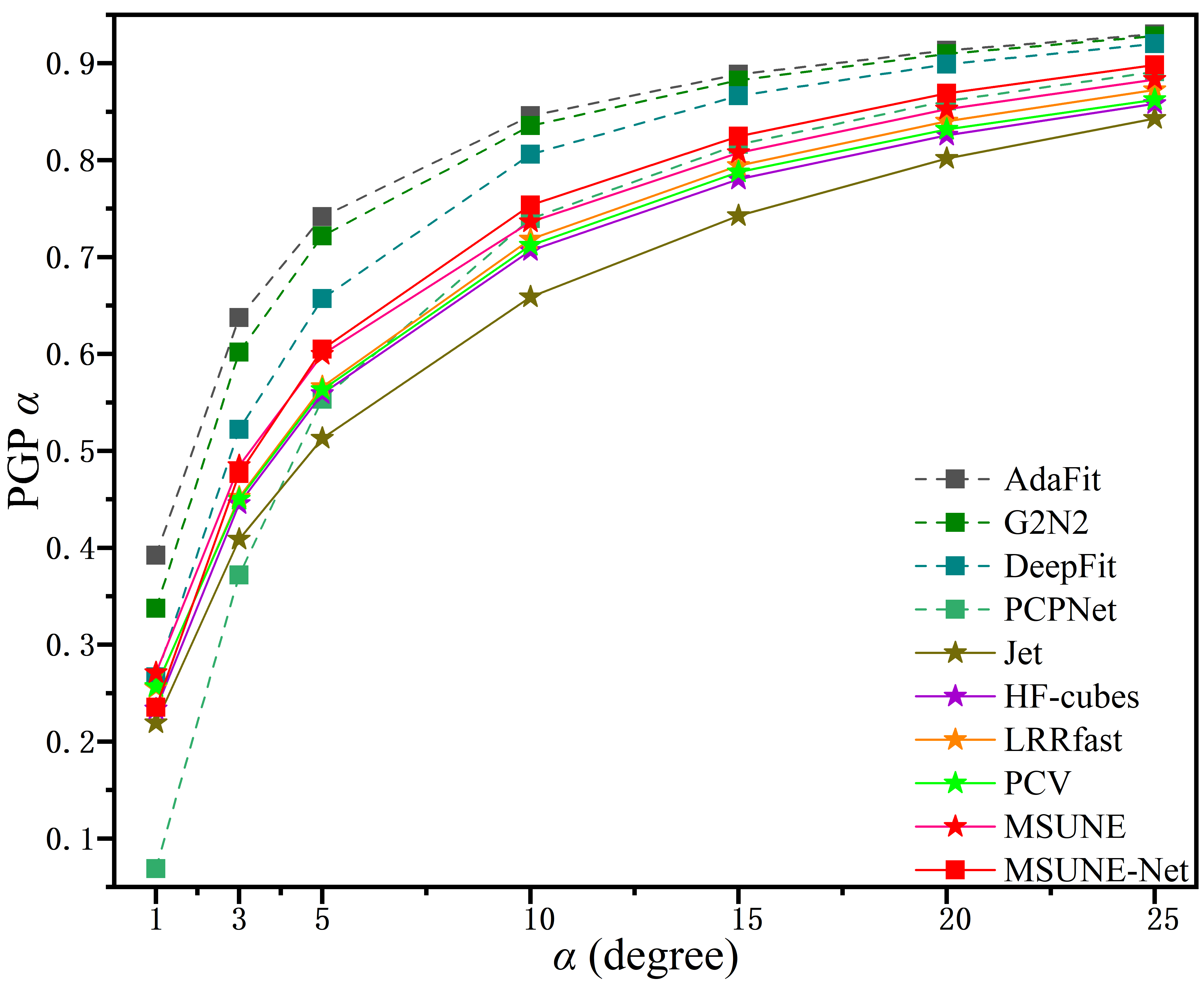
Figure 7: Comparison of PGP$\alpha$ on the synthetic dataset of PCPNet. MSUNE-Net surpasses previous conventional methods and is superior to PCPNet when $\alpha>10$.

\begin{overpic}[width=433.62pt,keepaspectratio]{Pclouds-v4.png} \par\put(3.4,17.5){0.4154/0.6792} \put(17.4,17.5){0.4258/0.6640} \put(31.2,17.5){0.5444/0.7882} \put(45.0,17.5){0.6038/0.8426} \put(58.9,17.5){0.5256/0.8067} \put(72.8,17.5){0.6005/0.8669} \put(86.0,17.5){{0.7089/0.9140}} \par\put(3.4,-1.0){0.1246/0.2333} \put(17.4,-1.0){0.1282/0.2358} \put(31.2,-1.0){0.1809/0.3090} \put(45.0,-1.0){0.1830/0.3133} \put(58.9,-1.0){0.2418/0.3699} \put(72.8,-1.0){0.2503/0.4232} \put(86.0,-1.0){{0.2930/0.4868}} \par\put(3.4,34.0){0.6183/0.8323} \put(17.4,34.0){0.6238/0.8401} \put(31.2,34.0){0.6754/0.7460} \put(45.0,34.0){0.7574/0.8666} \put(58.9,34.0){0.8361/0.9146} \put(72.8,34.0){0.8200/0.9582} \put(86.0,34.0){{0.8583/0.9607}} \par\put(6.6,-3.5){\small PCA} \put(21.1,-3.5){\small Jet} \put(34.4,-3.5){\small PCV} \put(46.7,-3.5){\small LRRFast} \put(60.1,-3.5){\small HF-cubes} \put(74.5,-3.5){\small PCPNet} \put(85.6,-3.5){\small MSUNE-Net} \par\put(98.0,0.8){0} \put(97.6,12.6){Up} \end{overpic}

Figure 8: Visual comparisons of the estimated normals on three models from the PCPNet dataset. Shapes are colored according to the normal angle error, where darker reds indicate larger errors and darker blues indicate smaller errors. Numerators and denominators are PGP5 and PGP10 of the results (higher is better).

6.2 Experiments on scanned data

In this section, three real scanned datasets, including two Kinect datasets and one LiDAR dataset, are utilized to evaluate our methods. Note that all the learning-based methods are only trained on the PCPNet dataset and directly evaluated on these three scanned datasets.

6.2.1 Evaluation on datasets scanned by Kinect

To begin with, we use two real datasets captured by a Kinect v1 RGBD camera to evaluate the generalization ability of our methods. The real scan data reveals more challenges, such as the fluctuation on flat surfaces, originating from the projection process of Kinect camera. The non-Gaussian and discontinuous noise make the scanned data have different noise patterns from the synthetic data. Specifically, its noise often has the same magnitude as some of the features [4, 40].

TABLE II: Comparison of RMS, RMS_τ, and PGP$\alpha$ on the Kinect dataset of PCV [1]. Both MSUNE and MSUNE-Net surpass previous conventional methods and deep learning methods.

Models	RMS	RMS_10	RMS_15	RMS_20	PGP10	PGP15	PGP20	PGP25
Sup.
AdaFit	18.38	66.25	54.17	44.32	0.4593	0.6421	0.7666	0.8495
G2N2	17.57	64.27	51.40	41.22	0.4909	0.6782	0.7993	0.8743
DeepFit	13.68	58.01	43.71	32.81	0.5853	0.7682	0.8753	0.9343
PCPNet	15.73	62.73	47.17	35.62	0.5155	0.7302	0.8527	0.9162
Unsup.
HF-cubes	11.72	43.99	31.79	24.73	0.7568	0.8747	0.9274	0.9536
LRRfast	13.25	48.36	34.23	26.84	0.7103	0.8573	0.9162	0.9452
PCV	11.74	46.85	31.81	23.85	0.7279	0.8768	0.9347	0.9607
MSUNE	11.67	49.54	33.64	24.51	0.6967	0.8628	0.9316	0.9620
MSUNE-Net	10.89	43.75	30.82	23.40	0.7614	0.8836	0.9363	0.9631

\begin{overpic}[width=433.62pt,keepaspectratio]{PCV-23-1-23.png} \par\put(14.2,37.6){16.54} \put(25.5,37.6){15.90} \put(36.7,37.6){11.85} \put(47.7,37.6){14.11} \put(58.9,37.6){12.03} \put(70.1,37.6){12.50} \put(81.4,37.6){11.73} \put(92.2,37.6){{10.31}} \par\put(14.2,-1.2){20.90} \put(25.5,-1.2){19.79} \put(36.7,-1.2){15.85} \put(47.7,-1.2){18.16} \put(58.9,-1.2){15.47} \put(70.1,-1.2){15.14} \put(81.4,-1.2){14.50} \put(92.2,-1.2){{13.45}} \par\put(13.4,-3.4){\small AdaFit} \put(25.1,-3.4){\small G2N2} \put(35.4,-3.4){\small DeepFit } \put(46.3,-3.4){\small PCPNet} \put(57.2,-3.4){\small HF-cubes} \put(68.8,-3.4){\small LRRfast} \put(81.3,-3.4){\small PCV} \put(89.8,-3.4){\small MSUNE-Net} \end{overpic}

Figure 9: Visual comparison of estimated normals by different methods on two statues scanned by Kinect from PCV [1]. Supervised deep normal estimators suffer from the scanner noise, i.e. the small fluctuations on smooth regions. The conventional methods can handle the fluctuations but may introduce artifacts around sharp features. MSUNE-Net works well for both two cases. Numbers show RMS of the results.

Dataset from PCV [1]. There are 71 scans in the training set and 73 scans in the test set. For each scan, a registered and reconstructed mesh from an Artec Spider^TM scanner (accuracy 0.5 mm) is used to help build ground truth normals. Although the annotations may not be correct or accurate enough, they provide one quantitative way to evaluate the methods at least.

Tab. II shows RMS, RMS_τ, and PGP$\alpha$ for the whole test set. Some visual comparisons of estimated normals rendered in RGB color are shown in Fig. 9. From Tab. II, we see that our methods achieve the lowest RMS and PGP errors. Moreover, we reveal an interesting phenomenon that, contrary to the results on the synthetic dataset, all supervised methods based on deep learning perform worse than the unsupervised methods. The higher the performance on the synthetic dataset, the lower the performance on the real dataset, as indicated by the RMS error of AdaFit, G2N2, and DeepFit in Tab. I and II. This phenomenon occurs mainly because the noise patterns of the synthetic and real scanned datasets are different. The deep learning-based supervised method misidentifies some noises as features, which destroys the structure of smooth regions, as shown in the results of AdaFit, G2N2, DeepFit, and PCPNet in Fig. 9. This also indicates that the generalization ability of supervised methods based on deep learning needs to be improved in essence.

The conventional methods, including HF-cubes, LRRfast, and PCV, handle the fluctuation introduced by the scanner better than supervised methods. While they tend to trigger off artifacts around sharp features, such as the noses of the two statues in Fig. 9. Our MSUNE-Net works well for both cases. It can better trade off features and smooth regions compared with other methods. This proves that our strategy has a stronger generalization ability.

\begin{overpic}[width=433.62pt,keepaspectratio]{NYUv2_cut.png} \put(14.1,-2.0){G2N2} \put(24.6,-2.0){DeepFit} \put(35.6,-2.0){AdaFit} \put(47.0,-2.0){PCPNet} \put(57.5,-2.0){HF-cubes} \put(69.1,-2.0){LRRfast} \put(81.5,-2.0){PCV} \put(89.5,-2.0){MSUNE-Net} \end{overpic}

Figure 10: Visual comparison of estimated normals on three scanned scenes from NYUV2. AdaFit, G2N2, and DeepFit can not suppress scanner noise. PCPNet and HF-cubes may fail to preserve tiny structures. LRRfast and PCV tend to introduce artifacts around high curvature regions. MSUNE-Net overcomes these challenges. After performing unoriented normal estimation, we flip normals according to the camera position. Colors encode the direction of oriented normals.

NYUV2 dataset. We also evaluate the performance of the proposed MSUNE-Net on NYUV2 dataset [21]. This dataset contains various indoor scenes without ground truth normals, so we only perform a qualitative comparison of various methods.

As shown in Fig. 10, AdaFit, G2N2, and DeepFit can preserve tiny details but with the price of retaining scanner noise. PCPNet and HF-cubes can well smooth noisy surfaces, but fail to preserve tiny details. LRRfast and PCV can capture some details and smooth the noisy surfaces, with the price of some erroneous normals in high curvature regions. Moreover, they are less practical due to longer runtime. MSUNE-Net copes with all these challenges. This experiment further illustrates that our method has better generalization performance.

6.2.2 Evaluation on LiDAR dataset

We further demonstrate our performance on the KITTI dataset, which is widely used in autonomous driving and has served as a public odometry and SLAM benchmark since 2012. The dataset provides sequentially organized point clouds collected by LiDAR with 64 beams. The experiments are conducted on the KITTI calibration sequence 2011-09-30. We use the corresponding ground truth device poses to splice out the whole scene, where the point cloud normals of every single frame are calculated and merged for the visualization in Fig. 1 and 11.

Compared with DeepFit, a cutting-edge supervised method, and PCA, the most widely used method, more geometry structures are preserved in the results of MSUNE-Net, as shown in Fig. 11. Many of them may facilitate further semantic analysis, such as the plane structures (third column), the sides of the vehicles (first and last columns), and tiny structures (second and third columns). MSUNE-Net also contributes to the more clear ground (second column) and wall (first column), since it can better prevent interference from closed objects.

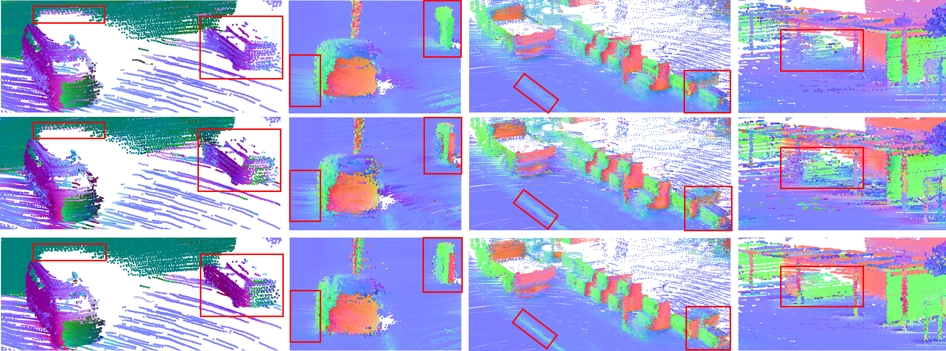
Figure 11: Visual comparison of estimated normals on four zoomed scenes of the KITTI dataset. MSUNE-Net identifies more geometry structures with higher quality. From top to bottom are PCA, DeepFit, and MSUNE-Net, respectively.

6.3 Efficiency

In Fig. 1, we report the average running time of different methods. Among them, the methods based on deep learning are implemented in Python 3.7.3. PCV and LRRfast are implemented in Matlab. HF-cubes is implemented in C++. DeepFit, G2N2, and MSUNE-Net have similar networks and inference times, and they are the fastest (about 0.3ms per point). PCPNet and AdaFit are a bit slower since they have more network parameters. Their inference time is 0.61ms and 0.71ms per point respectively. The conventional high-quality methods exhibit more generalization ability compared with the deep supervised methods. But they usually are more time-consuming. MSUNE-Net, a deep network-based unsupervised method, integrates the merits of the two approaches.

6.4 Ablation study

Validation of construction factors for candidate normals. Three important factors that may affect the quality of candidate normals are examined: multi-candidate sampling (MCS), adaptive neighborhood size (ANS), and candidate rejection (CR). We remove them to explore their influence on normal estimation. Without MCS, a single candidate normal, fitting all the neighbor points by PCA, is used to train the network. In the absence of ANS, we set the neighborhood size to a fixed value of 256. In order to better observe the influence of candidate normals, instead of using the candidate consensus loss and feature loss, we use a more general loss function $L_{pre}$ to describe the difference between the predicted normal and candidate normals at each query point:

$$L_{pre}=\sum_{\theta}\|\hat{\mathbf{n}}_{t}\times\mathbf{n}^{t}_{\theta}\|_{F}^{2},$$ (7)

where $\mathbf{n}^{t}_{\theta}$ represents the candidate normals which can be a single normal (without MCS), initial candidates (without CR), or feasible candidates (with CR).

Four ablation studies about the three factors are reported in lines 1 to 4 of Tab. III. Line 1 shows that training a network from a conventional method may exceed the conventional method itself. Specifically, if we use the results of PCA with 256 neighbors as a guide, the network still achieves slightly better performance (0.24 lower RMS angle error) than the former (the results of PCA are shown in Tab. I). After adding MCS, the RMS angle error is 0.78 lower than the PCA method with 256 neighbor points, which illustrates that learning from multi-candidate normals is superior to that from a single normal. Among these three factors, ANS plays an important role, which further reduces the RMS angle error by 1.67 and down to 14.79. CR can further improve the quality of candidate normals by rejecting the blurry normals in the initial candidate normals, which reduces the RMS angle error by 0.51.

TABLE III: Ablation study of MSUNE-Net on the dataset of PCPNet.

MCS	ANS	CR	$L_{ccn}$	$L_{w}$	RMS
					17.00
✓					16.46
✓	✓				14.79
✓	✓	✓			14.28
✓	✓		✓		14.17
✓	✓			✓	14.65
✓	✓		✓	✓	14.03
✓	✓	✓	✓		13.97
✓	✓	✓		✓	13.73
✓	✓	✓	✓	✓	13.57

Validation of loss terms. The contribution of $L_{ccn}$ and $L_{w}$ is illustrated in line 5 to 10 of Tab. III. When $L_{ccn}$ is disabled, $L_{pre}$ defined in Eq. 7 is used to make sure that the network can still learn from the candidate normals. The role of CR is similar to $L_{ccn}$ in deleting or weakening infeasible candidate normals, but they are actually complementary. To validate this, we divide the experiments into two groups: without CR (lines 5 to 7 of Tab. III) and with CR (lines 8 to 10 of Tab. III). It is found that both $L_{ccn}$ and $L_{w}$ further boost the performance of MSUNE-Net. The contribution of $L_{ccn}$ is more than that of $L_{w}$ in the absence of CR, and the effect is reversed when CR is introduced.

TABLE IV: Comparisons of the RMS angle error and inference time of MSUNE and MSUNE-Net with varying number of candidate normals on PCPNet’s synthetic dataset.

	MSUNE				MSUNE-Net
Number of candidate normals	20	100	400	4000	20	50	100	200
Average RMS	17.23	14.86	14.21	\	13.94	13.79	13.57	13.62
RMS on a noise-free point cloud	6.07	5.56	5.36	5.33	4.65	4.45	4.39	4.51
RMS on a point cloud with high noise	35.17	31.40	30.68	30.36	30.07	30.04	30.03	29.97
Inference time (ms) per point	85.45	103.26	167.44	936.79	0.36	0.36	0.36	0.36

Validation of the number of candidate normals. In Section 4.1, we construct multi-candidate normals by randomly picking points multiple times. In theory, the more candidate normals, the closer the empirical distribution is to the actual distribution. Thus, the higher the quality of normals learned by MSUNE/MSUNE-Net. This is consistent with our experiments in Tab. IV. For MSUNE, when the number of candidate normals is set to 4000, the time consumption is too high. Therefore, we just show its results on a noise-free point cloud and a point cloud with high noise. Since MSUNE predicts the normal for each point independently, it just learns from its own candidates. Therefore, MSUNE needs more candidate normals per point, even 4000 may not be enough. While MSUNE-Net can ”see” other candidate normals of similar neighborhoods during training. Thus its performance is better than that of MSUNE, even if there are far fewer candidates at each point. When the number of candidate normals increases to 100, the performance achieves its bound. Compared with MSUNE, MSUNE-Net has also another advantage in that it is ultra-fast since no candidate normals or any optimization are necessary for network inference.

7 An implementation of the paradigm to unsupervised point cloud denoising

The proposed multi-sample consensus paradigm is also applicable to other unsupervised tasks. This is shown by improving the cutting-edge unsupervised point cloud denoising method: DMR [20]. DMR follows the unsupervised denoising loss defined in [19]:

$$L_{U}=\frac{1}{N}\sum_{t=1}^{N}\sum_{q}\|f(p_{t})-q\|,$$ (8)

where $f(\cdot)$ represents the denoiser that maps a noisy point to a denoised point. Points $\{q\}$ are sampled from the noisy input point cloud $P$ according to a prior $P(q|p_{t})$, which is empirically defined as:

$$P(q|p_{t})\propto exp(-\frac{\|q-p_{t}\|}{2\omega^{2}}).$$ (9)

Then the sampling point $q$ is closer to the underlying clean surface with high probability. However, it is not a suitable assumption for points around the sharp features. Although Hermosilla et al. [19] employ RGB color annotation to overcome this problem, it is just alleviated but not eliminated. Moreover, RGB color annotation is not always available. The idea of candidate rejection and mode determination can be employed to overcome this problem. Besides we design a novel sampling strategy to generate multiple more accurate $\{q\}$ to guide the network training.

Multi-candidate sampling (MCS). Instead of sampling $q$ from the input noisy point cloud $P$ directly, we first randomly select $k_{s}=4$ points in the $\hat{k}$ nearest neighbors of $p_{t}$ and take their center as a candidate $q$. This progress is repeated multiple times to obtain a set of candidates $\{q\}$. $\hat{k}=64$ is the same as DMR.

Candidate rejection (CR). A candidate is infeasible if there are fewer neighbors of $p_{t}$ near it. Therefore, we compute a score for each candidate:

$$s^{t}_{q}=\sum_{i=1}^{\hat{k}}e^{-\frac{\left(d(\mathbf{p}_{t}^{i},q)\right)^{2}}{\sigma^{2}}},$$ (10)

where $\mathbf{p}_{t}^{i}\in\mathcal{N}_{\hat{k}}(p_{t})$ is a neighbor of $\mathbf{p}_{t}$, $d(\mathbf{p}_{t}^{i},q)$ represents the Euclidean distance from $\mathbf{p}_{t}^{i}$ to $q$, and $\sigma$ is the bandwidth of the Gaussian kernel function. In the experiments, we set $\sigma$ equal to the average distance of the 12 nearest neighbor points of $\mathbf{p}_{t}$. Then the 10% of initialized candidates with lower scores are deleted.

TABLE V: The denoising performance of DMR is gradually improved by applying our strategies.

Noise scale	1$\%$		2$\%$		2.5$\%$		3$\%$
Error metric	CD	P2S	CD	P2S	CD	P2S	CD	P2S
DMR	2.47	2.97	4.01	5.58	4.92	7.20	5.77	8.73
DMR+MCS	2.38	2.84	3.74	5.15	4.61	6.65	5.49	8.24
DMR+MCS+$L_{ccp}$	2.13	2.43	3.54	4.75	4.42	6.25	5.27	7.78
DMR+MCS+$L_{ccp}$+CR	2.13	2.41	3.47	4.60	4.28	6.00	5.08	7.42

Mode determination. A candidate consensus loss for position, similar with $L_{ccn}$, is defined as follows:

$$L_{ccp}=\sum_{q}-e^{-\frac{\left\|f(p_{t})-q\right\|_{F}^{2}}{\tau^{2}}},$$ (11)

where $\tau{\color[rgb]{0,0,0}=\sigma}$. This results in convergence to the main mode supported by more inlier candidates.

Dataset. For training the denoising network, we have collected 13 different classes with 7 different meshes, each from ModelNet-40 [46], and generate point clouds by randomly sampling 10K-50K points. The point clouds are then perturbed by Gaussian noise with standard deviations from 1% to 3% of the bounding box diagonal. Finally, a training dataset containing a total of 1365 models was generated. To be identical to the DMR training mechanism, we split the point cloud into patches consisting of 1024 points. For testing, we have collected 20 classes with 3 meshes each. Similarly, we generate point clouds using randomly sampled 20K and 50K points, then perturb them by Gaussian noise with standard deviations of 1%, 2%, 2.5%, and 3% of the bounding box diagonal. Finally, a test dataset containing 480 models was generated.

Results. We evaluate the effectiveness of our strategies quantitatively and qualitatively on the dataset. For quantitative comparison, the Chamfer distance (CD) and point-to-surface distance (P2S) are used as evaluation metrics. As shown in Tab. V, the CD and P2S are gradually improved by applying the three strategies. A qualitative comparison is also shown in Fig. 12, where the colors encode the P2S errors. Our results are much cleaner and exhibit more visually pleasing surfaces than those of DMR.

\begin{overpic}[width=216.81pt,keepaspectratio]{denoise.png} \put(4.0,-2.5){Raw point cloud} \put(44.8,-2.5){DMR} \put(79.7,-2.5){Our} \par\put(96.5,0.6){0 \footnotesize} \put(95.9,21.1){Up \footnotesize} \end{overpic}

Figure 12: More visually pleasing surfaces are generated by the proposed unsupervised denoising method (DMR+MCS+$L_{ccp}$+ CR) than the baseline method: DMR. The colors, from blue to red, encode the P2S error.

8 Conclusion

In this paper, we propose a multi-sample consensus paradigm for unsupervised normal estimation and two implementations of it: a novel optimization method (MSUNE) and the first unsupervised deep normal estimation method (MSUNE-Net). The paradigm consists of three stages: multi-candidate sampling, candidate rejection, and mode determination. It is completely generalizable for other unsupervised low-level image and point cloud processing. A preliminary implementation of the paradigm to unsupervised point cloud denoising is also introduced.

We prove that the normal of each query point of a noisy point cloud is the expectation of randomly sampled candidate normals ideally. But they are actually from a multimodal distribution. Hence, MSUNE presents practicable strategies on how to sample multiple candidates, reject some infeasible ones, and determine the main mode of the candidates. The performance of MSUNE increases with the number of candidate normals. It is superior to the SOTA optimization methods and supervised deep normal estimators on real data. But the per-point optimization is very time-consuming.

MSUNE-Net further introduces a neural network to boost the multi-sample consensus paradigm. With the assistance of training on massive data, the patch self-similarity across point clouds is adequately utilized, which provides far more candidate normals for each query point with similar patches implicitly. Higher performance is accomplished by MSUNE-Net even with smaller candidates set per point, and it is also 100 times faster than MSUNE. MSUNE-Net is even superior to some supervised deep normal estimators on the most common synthetic dataset. Most importantly, it shows better generalization ability and significantly outperforms previous optimization methods and SOTA supervised deep normal estimators on three real datasets.

In the future, we intend to conduct in-depth research in low-level image and point cloud analysis via unsupervised deep learning driven by multi-sample consensus. It would also be interesting to explore how to generate and use multiple pseudo-labels for semantic-level unsupervised learning tasks.

Jie Zhang received the PhD degree in 2015 from the Dalian University of Technology, China. She is currently an associate professor with the School of Mathematics, Liaoning Normal University, China. Her current research Interests include geometric processing and machine learning.

Minghui Nie is a master student in computational mathematics at Liaoning Normal University, China. He received the bachelor’s degree in mathematics and applied mathematics at Dezhou University, China, in 2021. His research interests include geometric processing and machine learning.

Junjie Cao received the BSc degree in 2003 and the PhD degree in 2010 from Dalian University of Technology, china. He is an associate professor with the School of Mathematical Sciences, Dalian University of Technology, China. Between 2014 and 2015, he paid an academic visit to Simon Fraser University, Canada. His research interests include geometric processing and image processing.

Jian Liu received the PhD degree in 2022 from the Shandong University, China. He is currently a postdoctor with the School of Software, Tsinghua University, China. His current research interests include geometric processing and machine learning.

Ligang Liu received the BSc degree in 1996 and the PhD degree in 2001 from Zhejiang University, China. He is a professor at the University of Science and Technology, China. Between 2001 and 2004, he was at Microsoft Research Asia. Then he was at Zhejiang University during 2004 and 2012. He paid an academic visit to Harvard University during 2009 and 2011. His research interests include geometric processing and image processing. His research works could be found at his research website: http://staff.ustc.edu.cn/ lgliu

References

- [1] J. Zhang, J. Cao, X. Liu, H. Chen, B. Li, and L. Liu, “Multi-normal estimation via pair consistency voting,” IEEE Transactions on Visualization and Computer Graphics, vol. 25, no. 4, pp. 1693–1706, 2019.
- [2] A. Geiger, P. Lenz, and R. Urtasun, “Are we ready for autonomous driving? the kitti vision benchmark suite,” in IEEE Conference on Computer Vision and Pattern Recognition, 2012, pp. 3354–3361.
- [3] P. Guerrero, Y. Kleiman, M. Ovsjanikov, and N. J. Mitra, “PCPNet: Learning local shape properties from raw point clouds,” Computer Graphics Forum, vol. 37, no. 2, pp. 75–85, 2018.
- [4] Y. Ben-Shabat and S. Gould, “DeepFit: 3d surface fitting via neural network weighted least squares,” in European Conference on Computer Vision, vol. 12346, 2020, pp. 20–34.
- [5] H. Zhou, H. Chen, Y. Zhang, M. Wei, H. Xie, J. Wang, T. Lu, J. Qin, and X.-P. Zhang, “Refine-Net: Normal refinement neural network for noisy point clouds,” IEEE Transactions on Pattern Analysis and Machine Intelligence, vol. 45, pp. 946–963, 2022.
- [6] R. Zhu, Y. Liu, Z. Dong, T. Jiang, Y. Wang, W. Wang, and B. Yang, “AdaFit: Rethinking learning-based normal estimation on point clouds,” in IEEE/CVF International Conference on Computer Vision, 2021, pp. 6118–6127.
- [7] Y. Ben-Shabat, M. Lindenbaum, and A. Fischer, “Nesti-Net: Normal estimation for unstructured 3d point clouds using convolutional neural networks,” in IEEE Conference on Computer Vision and Pattern Recognition, 06 2019, pp. 10 104–10 112.
- [8] J. Zhang, J.-J. Cao, H.-R. Zhu, D.-M. Yan, and X.-P. Liu, “Geometry guided deep surface normal estimation,” Computer-Aided Design, vol. 142, no. 103119, 2022.
- [9] J. E. Lenssen, C. Osendorfer, and J. Masci, “Deep iterative surface normal estimation,” in IEEE/CVF Conference on Computer Vision and Pattern Recognition, 2020, pp. 11 244–11 253.
- [10] Q. Li, Y.-S. Liu, J.-S. Cheng, C. Wang, Y. Fang, and Z. Han, “HSurf-Net: Normal estimation for 3d point clouds by learning hyper surfaces,” in Advances in Neural Information Processing Systems, 2022.
- [11] H. Hoppe, T. DeRose, T. Duchamp, J. A. McDonald, and W. Stuetzle, “Surface reconstruction from unorganized points,” in Annual Conference on Computer Graphics and Interactive Techniques, 1992, pp. 71–78.
- [12] J. Zhang, J. Cao, X. Liu, J. Wang, J. Liu, and X. Shi, “Point cloud normal estimation via low-rank subspace clustering,” Computers & Graphics, vol. 37, no. 6, pp. 697–706, 2013.
- [13] B. Li, R. Schnabel, R. Klein, Z. Cheng, G. Dang, and S. Jin, “Robust normal estimation for point clouds with sharp features,” Computers & Graphics, vol. 34, no. 2, pp. 94–106, 2010.
- [14] A. Boulch and R. Marlet, “Fast and robust normal estimation for point clouds with sharp features,” Computer Graphics Forum, vol. 31, no. 5, p. 1765–1774, 2012.
- [15] F. Cazals and M. Pouget, “Estimating differential quantities using polynomial fitting of osculating jets,” in Computer Aided Geometric Design, 2005, pp. 121–146.
- [16] X. Liu, J. Zhang, J. Cao, B. Li, and L. Liu, “Quality point cloud normal estimation by guided least squares representation,” Computers & Graphics, vol. 51, pp. 106–116, 2015.
- [17] J. Lehtinen, J. Munkberg, J. Hasselgren, S. Laine, T. Karras, M. Aittala, and T. Aila, “Noise2noise: Learning image restoration without clean data,” in International Conference on Machine Learning, 2018, pp. 4620–4631.
- [18] J. Batson and L. Royer, “Noise2self: Blind denoising by self-supervision,” in International Conference on Machine Learning, 2019, pp. 524–533.
- [19] P. H. Casajus, T. Ritschel, and T. Ropinski, “Total denoising: Unsupervised learning of 3d point cloud cleaning,” in IEEE/CVF International Conference on Computer Vision, 2019, pp. 52–60.
- [20] S. Luo and W. Hu, “Differentiable manifold reconstruction for point cloud denoising,” in ACM International Conference on Multimedia, 2020, pp. 1330–1338.
- [21] N. Silberman, D. Hoiem, P. Kohli, and R. Fergus, “Indoor segmentation and support inference from RGBD images,” in European Conference on Computer Vision, vol. 7576, 2012, pp. 746–760.
- [22] D. Levin, “The approximation power of moving leastsquares,” Mathematics of computation, vol. 67, no. 224, p. 1517–1531, 1998.
- [23] N. J. Mitra, A. Nguyen, and L. J. Guibas, “Estimating surface normals in noisy point cloud data,” Annual Symposium on Computational Geometry, pp. 322––328, 2003.
- [24] G. Guennebaud and M. Gross, “Algebraic point set surfaces,” ACM Transactions on Graphics, vol. 26, no. 3, pp. 23.1–23.9, 2007.
- [25] N. Amenta and M. W. Bern, “Surface reconstruction by voronoi filtering,” Discrete & Computational Geometry, vol. 22, no. 4, pp. 481–504, 1999.
- [26] T. K. Dey and S. Goswami, “Provable surface reconstruction from noisy samples,” Annual Symposium on Computational Geometry, p. 330–339, 2004.
- [27] P. Alliez, D. Cohen-Steiner, Y. Tong, and M. Desbrun, “Voronoi-based variational reconstruction of unoriented point sets,” in Symposium on Geometry Processing, 2007, p. 39–48.
- [28] Q. Merigot, M. Ovsjanikov, and L. J. Guibas, “Voronoi-based curvature and feature estimation from point clouds,” in IEEE Transactions on Visualization and Computer Graphics, 2010, p. 743–756.
- [29] P. Luo, Z. Wu, C. Xia, L. Feng, and B. Jia, “Robust normal estimation of point cloud with sharp features via subspace clustering,” in International Conference on Graphic and Image Processing, vol. 9069, 2014, pp. 346–351.
- [30] S. Fleishman, D. Cohen-Or, and C. T. Silva, “Robust moving least-squares fitting with sharp features,” ACM Transactions on Graphics, vol. 24, no. 3, pp. 544–552, 2005.
- [31] M. Yoon, Y. Lee, S. Lee, I. P. Ivrissimtzis, and H. Seidel, “Surface and normal ensembles for surface reconstruction,” Computer-Aided Design, vol. 39, no. 5, pp. 408–420, 2007.
- [32] B. Mederos, L. Velho, and L. H. de Figueiredo, “Robust smoothing of noisy point clouds,” in Siam conference on geometric design and computing, 2003.
- [33] Y. Wang, H.-Y. Feng, F.-É. Delorme, and S. Engin, “An adaptive normal estimation method for scanned point clouds with sharp features,” Computer-Aided Design, vol. 45, no. 11, pp. 1333 – 1348, 2013.
- [34] J. Wang, K. Xu, L. Liu, J. Cao, S. Liu, Z. Yu, and X. D. Gu, “Consolidation of low-quality point clouds from outdoor scenes,” Computer Graphics Forum, vol. 32, pp. 207–216, 2013.
- [35] A. Boulch and R. Marlet, “Deep learning for robust normal estimation in unstructured point clouds,” in Computer Graphics Forum, vol. 35, 2016, pp. 281–290.
- [36] R. Roveri, A. C. Oztireli, I. Pandele, and M. H. Gross, “Pointpronets: Consolidation of point clouds with convolutional neural networks,” Computer Graphics Forum, vol. 37, no. 2, p. 87–99, 2018.
- [37] J. Zhou, H. Huang, B. Liu, and X. Liu, “Normal estimation for 3d point clouds via local plane constraint and multi-scale selection,” Computer Aided Geometric Design, vol. 129, p. 102916, 2020.
- [38] T. Hashimoto and M. Saito, “Normal estimation for accurate 3d mesh reconstruction with point cloud model incorporating spatial structure,” in IEEE/CVF Conference on Computer Vision and Pattern Recognition Workshops, 2019, pp. 54–63.
- [39] F. Pistilli, G. Fracastoro, D. Valsesia, and E. Magli, “Point cloud normal estimation with graph-convolutional neural networks,” in IEEE International Conference on Multimedia & Expo Workshops, 2020, pp. 1–6.
- [40] H. Zhou, H. Chen, Y. Feng, Q. Wang, J. Qin, H. Xie, F. L. Wang, M. Wei, and J. Wang, “Geometry and learning co-supported normal estimation for unstructured point cloud,” in IEEE/CVF Conference on Computer Vision and Pattern Recognition, 2020, pp. 13 235–13 244.
- [41] K. Li, M. Zhao, H. Wu, D.-M. Yan, Z. Shen, F.-Y. Wang, and G. Xiong, “Graphfit: Learning multi-scale graph-convolutional representation for point cloud normal estimation,” in European Conference on Computer Vision, 2022, pp. 651–667.
- [42] D.-H. Lee, “Pseudo-label: The simple and efficient semi-supervised learning method for deep neural networks,” in Workshop on Challenges in Representation Learning, vol. 3, no. 2, 2013, p. 896.
- [43] D. Berthelot, N. Carlini, I. Goodfellow, N. Papernot, A. Oliver, and C. A. Raffel, “Mixmatch: A holistic approach to semi-supervised learning,” Advances in Neural Information Processing Systems, vol. 32, p. 5049–5059, 2019.
- [44] A. Tarvainen and H. Valpola, “Mean teachers are better role models: Weight-averaged consistency targets improve semi-supervised deep learning results,” Advances in Neural Information Processing Systems, vol. 30, p. 1195–1204, 2017.
- [45] A. Krull, T.-O. Buchholz, and F. Jug, “Noise2void-learning denoising from single noisy images,” in IEEE/CVF Conference on Computer Vision and Pattern Recognition, 2019, pp. 2129–2137.
- [46] Z. Wu, S. Song, A. Khosla, F. Yu, L. Zhang, X. Tang, and J. Xiao, “3D ShapeNets: A deep representation for volumetric shapes,” in IEEE Conference on Computer Vision and Pattern Recognition, 2015, pp. 1912–1920.