Integrable Feynman Graphs and Yangian Symmetry on the Loom

Abstract

We extend the powerful property of Yangian invariance to a new large class of conformally invariant Feynman integrals. Our results apply to planar Feynman diagrams in any spacetime dimension dual to an arbitrary network of intersecting straight lines on a plane (Baxter lattice), with propagator powers determined by the geometry. We formulate Yangian symmetry in terms of a chain of Lax operators acting on the fixed coordinates around the graph, and we also extend this construction to the case of infinite-dimensional auxiliary space. Yangian invariance leads to new differential and integral equations for individual, highly nontrivial, Feynman graphs, and we present them explicitly for several examples. The graphs we consider determine correlators in the recently proposed loom fishnet CFTs. We also describe a generalization to the case with interaction vertices inside open faces of the diagram. Our construction unifies and greatly extends the known special cases of Yangian invariance to likely the most general family of integrable scalar planar graphs.

1 Introduction

Yangian symmetry for quantum integrable systems is an old and well established subject Faddeev:1996iy ; molev2007yangians ; Bernard:1992ya ; MacKay:2004tc ; Loebbert:2016cdm . In physics, besides spin chains, one of the most important uses of the Yangian symmetry concerns the planar scattering amplitudes in $N=4$ supersymmetric Yang-Mills theory or in ABJM theory where it is closely linked with dual conformal symmetry Drummond:2009fd ; Drummond:2008vq ; Beisert:2010gn ; Arkani-Hamed:2012zlh ; Huang:2010qy ; Bargheer:2010hn . However its application to planar conformal Feynman graphs is a rather recent observation Chicherin:2017cns ; Chicherin:2017frs (see also Chicherin:2013sqa ). As a powerful and rather general tool, Yangian symmetry can have far-reaching consequences, both for the formal development of quantum integrability as well as for practical calculation of interesting physical quantities: specific Feynman graphs and planar scattering amplitudes, partition functions of integrable statistical mechanical systems with spins fixed at arbitrary boundaries, as well as for the analysis of moduli space of Calabi-Yau manifolds Duhr:2022pch . Some new developments stemming from these implementations of Yangian symmetry can be found in Loebbert:2019vcj ; Loebbert:2020hxk ; Loebbert:2020tje ; Loebbert:2020glj ; Corcoran:2020epz ; Corcoran:2021gda , see Loebbert:2022nfu ; Chicherin:2022nqq for a review. This symmetry is expected to be of particular importance for the fishnet CFTs, first discovered in Gurdogan:2015csr as a special scaling limit of the $\gamma$-deformed $\mathcal{N}=4$ Super-Yang-Mills theory (see  Caetano:2016ydc ; Kazakov:2018hrh for a review). The fishnet theories were later generalized to the fishnet reduction of 3d ABJM theorys Caetano:2016ydc and to other spacetime dimensions and deformations Kazakov:2018qbr ; Mamroud:2017uyz and finally to the most general setup – the loom fishnet CFTs Kazakov:2022dbd . The graph content of these fishnet CFTs is based on the old construction of A. Zamolodchikov Zamolodchikov:1980mb for the most general integrable planar conformal Feynman diagrams, which he considered as a specific statistical mechanical model. Based on this integrability of the underlying Feynman graphs, many physical results have been found for these fishnet CFTs, for various quantities and in various dimensions Derkachov:2021ufp ; Derkachov:2021rrf ; Derkachov:2020zvv ; Derkachov:2019tzo ; Kazakov:2018gcy ; Derkachov:2018rot ; Kazakov:2018qbr ; Caetano:2016ydc ; Gromov:2018hut ; Gromov:2019aku ; Gromov:2017cja ; Grabner:2017pgm ; Basso:2018cvy ; Basso:2018agi ; Basso:2017jwq ; Mamroud:2017uyz ; Cavaglia:2021mft ; Pittelli:2019ceq ; Kostov:2022vup ; Ferrando:2023ogg .

Yangian symmetry gives a remarkable realization of integrability at the level of an individual Feynman graph. It has been used successfully in order to obtain a variety of new results for nontrivial conformal Feynman integrals, with the first direction explored Chicherin:2017cns ; Chicherin:2017frs being arbitrary graphs in the original 4d fishnet theories where the graphs are cut out from a regular square lattice. These results were later generalized to specific examples in other dimensions and/or with generic propagator powers Loebbert:2019vcj ; Corcoran:2021gda ; Duhr:2022pch . More generally, in Chicherin:2022nqq ; Loebbert:2020hxk it was suggested that conformal graphs in any dimensions cut out from regular tilings of the plane should have Yangian symmetry. At the same time, a unified picture of what is the full class of graphs with Yangian symmetry has been missing, and the exploration of this powerful property has been done mostly on a case-by-case basis.

In this work, we will establish the Yangian symmetry of the most general planar Feynman diagrams built via Zamolodchikov’s integrability construction based on star-triangle relations. Our method will be an extension of the “lasso” method formulated in Chicherin:2017cns ; Chicherin:2017frs for particular case of 4d planar graphs of disc topology cut out of the regular square lattice, though the details of this generalization are rather tricky. We extend it to the case when the graph is built starting from a general (and not necessarily regular) lattice dual to the so-called Baxter lattice baxter1978solvable – an arbitrary collection of intersecting straight lines that provide a checkerboard coloring of the plane, see figure 1 . The scaling dimensions of the propagators are expressed via the angles at which the lines intersect. This geometric construction ensures that the graphs are finite and conformal (i.e. the sum of scaling dimensions at each vertex is $D$), and in addition imposes further linear constraints on the propagator powers so that not all conformal graphs are integrable in the sense we discuss. As an outcome, the graph is shown to be an eigenstate of the ’lasso’ monodromy matrix constructed as a chain of conformal Lax operators known from Chicherin:2012yn .

In order to demonstrate Yangian invariance, we gradually remove the lasso, i.e. the chain of Lax operators, from the Feynman diagram step by step, extending the approach of Chicherin:2017cns ; Chicherin:2017frs . In the process we use a variety of nontrivial identities for the conformal Lax operators. We have managed to rigorously prove the validity of several steps in this (in general quite complex) procedure by invoking a number of geometric arguments based on the way the graph is constructed from the Baxter lattice. We expect that the procedure should apply to an arbitrary Feynman graph constructed in this way.

We also further extend the class of admissible Feynman graphs by generalising the construction of Zamolodchikov:1980mb ; Kazakov:2022dbd – namely, allowing the interaction vertices to be placed inside external open faces of the lattice. We give more details on this in section 2.1.

As a main result, we will derive, expanding in inverse powers of the spectral parameter, the linear Yangian differential equations on these graphs. The equations have a pretty universal form and are distinguished only by different sets of evaluation parameters for different graphs. Such equations have been obtained before for various particular graphs, and in many cases were shown to be rather powerful as they restrict the graph to be a linear combination of a finite set of basis functions. This has already led to the calculation of several graphs including first the general cross and then the double cross for which the result is highly involved and was found only recently Loebbert:2019vcj ; Ananthanarayan:2020ncn . We hope that our results will open the way to exploration of more general Feynman integrals.

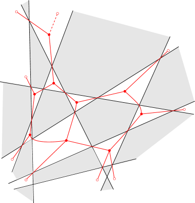
Figure 1: Example of a Feynman graph generated via the loom construction. The propagators are shown as red lines, the internal vertices filled red circles, and the external points as empty red circles. Black lines form the original Baxter lattice which is painted in the checkerboard manner – the loom. To each internal vertex or external point we assign a $D$-dimensional coordinate and integrate over those of the internal points. At the top left we show one generalisation we have made to the standard construction, namely a vertex inside an open external face with an extra dashed propagator (more details in section 2.1).

Furthermore, we managed to construct the lasso operator, i.e. the chain of Lax matrices, with a noncompact representation in the auxiliary space (instead of the compact one mentioned above), the same as the principal series representation of $D$-dimensional conformal algebra in the quantum space. The corresponding R-matrix out of which our lasso is made has been known for quite a while Chicherin:2012yn . The statement that the graph is an eigenfunction of this lasso of R-matrices is now an integral rather than a differential equation. Furthermore, the R-matrix itself is simply a product of four propagators with weights containing the spectral parameter, which means that our construction not only gives new integral equations for the graph but also represents an interesting equivalence between various Feynman diagrams.

The paper is organized as follows. In section 2 we review Zamolodchikov’s construction of Feynman graphs based on the loom – the Baxter lattice – and describe our generalisation of it. In section 3 we review the conformal Lax operators and their key properties. In section 4 we describe the lasso construction which leads to Yangian invariance of the graphs and its extension to our general case, with a rather intricate proof of several steps in the process of removing the chain of Lax operators from the diagram. In section 5 we present the general form of the differential equations for Feynman integrals which follow from Yangian invariance, as well as some explicit examples. In section 6 we describe another nontrivial generalisation of the construction, namely the case of infinite-dimensional auxiliary space and the resulting integral equations for graphs. We present conclusions and future directions in section 7.

2 Integrable Feynman graphs from the loom

The Feynman graphs we discuss in this paper are coordinate-space planar diagrams obtained from the construction originally proposed by Zamolodchikov in Zamolodchikov:1980mb . Let us first discuss here this construction in detail, for completeness, and then in section 2.1 we will describe a certain generalisation of it that we will also explore.

The starting point is a Baxter lattice – a finite set of intersecting lines on the plane. Some lines may be parallel to each other but triple or higher intersections are not allowed. Such a set of lines divides the plane into a set of polygonal faces which admit a checkerboard coloring, and accordingly we will draw them as white or grey. The actual Feynman diagram is drawn on the graph which is dual to the lattice of the white faces. The rules are as follows:

• Inside any white face which is a closed polygon one may place an internal vertex of the Feynman graph. In this case we draw propagators going from this vertex to each of its neighboring white faces and passing through the angles of this polygon. To each internal vertex we associate a $D$-dimensional coordinate which is to be integrated over.

• A propagator coming out of an internal vertex can be either an external leg of the diagram, or it can connect to the internal vertex in the neighboring white face.

• The propagator connecting two points $x_{1}$ and $x_{2}$ is given by the conformal 2-pt function

  $$\frac{1}{|x_{1}-x_{2}|^{2\Delta}}\ ,$$ (1)

  and, crucially, the scaling dimension $\Delta$ is determined by the angle of the polygon through which the propagator passes as (see figure 2)

  $$\Delta=D\frac{\pi-\alpha}{2\pi}\ .$$ (2)

As a result we obtain a Feynman diagram given by a multipoint integral in coordinate space with propagators of the form (1).

Remarkably, the sum of scaling dimensions for propagators at each vertex is $D$ due to the geometric constraint on the sum of the angles of any closed polygon. To see this, notice that $\pi-\alpha$ in (2) is the external angle at the vertex of the polygon, and the sum of all such angles for an $n$-gon is $\pi n-\pi(n-2)=2\pi$ (regardless of $n$). Thus the resulting Feynman integral is always a conformal object. We show an example of such a Feynman graph on figure 1 in the Introduction.

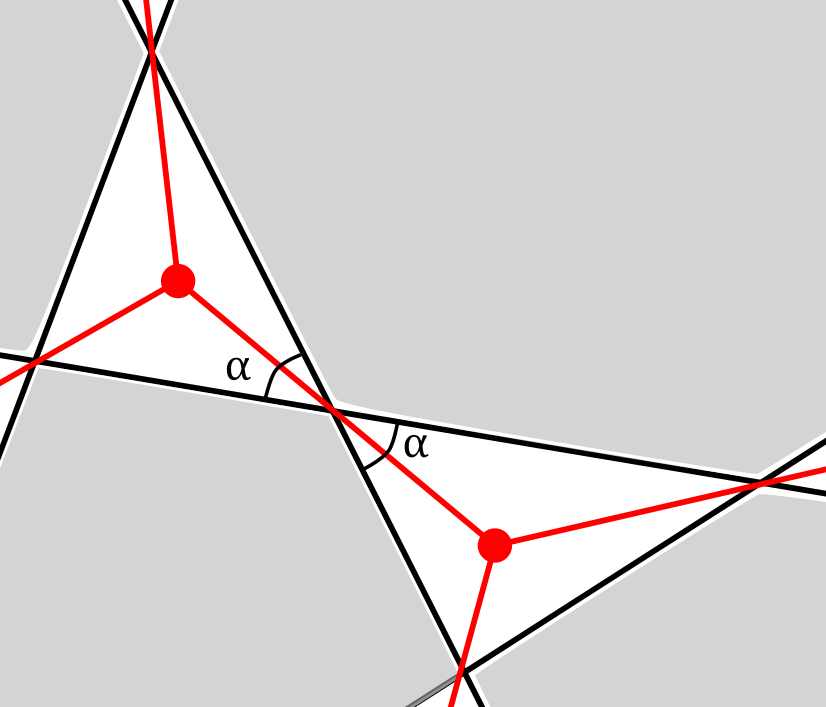
Figure 2: Fragment of a Feynman graph. The propagator between points $x_{1},x_{2}$ is given by $(x_{1}-x_{2})^{-2\Delta}$ with the power determined by the angle $\alpha$ through which it passes according to $\Delta=D\frac{\pi-\alpha}{2\pi}$.

Figure 3: A simple Feynman graph with one internal vertex and three external points.

The simplest example is a 1-point integral with three external legs, shown on figure 3. It is given by

$$I=\int d^{d}x\frac{1}{|x_{1}-x|^{2\Delta_{1}}|x_{2}-x|^{2\Delta_{2}}|x_{3}-x|^{2\Delta_{3}}}\ ,$$ (3)

where $\Delta_{k}=D\frac{\pi-\alpha_{k}}{2\pi}$ are fixed in terms of the three angles of the triangle. This integral can be computed via the star-triangle relation that we review below (equation (4)).

So far we have defined these Feynman graphs just as explicit multipoint integrals, without regard to any particular field theory. However, it was recently understood in Kazakov:2022dbd that there does exist a large family of Lagrangian field theories, dubbed as loom fishnet CFTs, whose Feynman diagrams that determine perturbative correlation functions of single trace operators are precisely these ones. This further motivates their deep investigation.

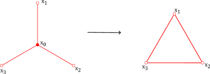
Figure 4: Graphic illustration of the star-triangle relation (4).

When working with these Feynman graphs it is often useful to utilise the star-triangle identity. It reads

$$\int d^{D}x_{0}\prod_{i=1}^{3}\frac{1}{|x_{i0}|^{2\Delta_{i}}}=\pi^{D/2}\prod_{i=1}^{3}\frac{\Gamma(D/2-\Delta_{i})}{\Gamma(\Delta_{i})}\prod_{i=1}^{3}\frac{1}{|x_{i-1}-x_{i+1}|^{2(D/2-\Delta_{i})}}\ ,$$ (4)

and holds when $\Delta_{1}+\Delta_{2}+\Delta_{3}=D$. We show it graphically on figure 4. Let us also mention that this identity has a very natural place in the setting we are considering since moving the lines of the Baxter lattice amounts to star-triangle transformations of the Feynman graph Zamolodchikov:1980mb . This fact itself may be viewed as a manifestation of the ‘integrability’ of these graphs.

2.1 Generalization to vertices inside external faces

In the construction we described above, internal vertices are only allowed inside faces that are closed polygons, and not inside the external open faces that go off to infinity. This is natural since the fixed sum of angles of a closed polygon guarantees that the sum of weights at each vertex is $D$ and the graph is conformal. In fact we found that this construction can be naturally extended also to the case when internal vertices are placed inside open faces. In this case one should simply add an extra propagator which completes the sum of conformal weights at the vertex to $D$. We draw these propagators as dashed lines, examples are given on figures 5, 6. Another example is given in the Introduction on figure 1 where a vertex of the new type is in the upper left corner.

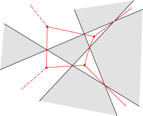
Figure 5: A generalized loom Feynman diagram with interaction vertices inside external faces. The Feynman graph is built out of propagators shown in red. Bold filled circles show internal integrated vertices, empty circles show the ends of external legs. The scaling dimensions for dashed lines are fixed by requiring the sum of dimensions at each vertex to be $D$, for the other lines they are fixed by geometry (see section 2).

Figure 6: A simple Feynman graph with interaction vertices inside external open faces. We have labelled in red the scaling dimensions for each propagator.

Notice that the new propagator will always have a positive scaling dimension as follows from geometry. That is, when we remove some edges from a closed polygon the sum of its external angles will become smaller than $2\pi$ which in terms of scaling dimensions means the sum of original $\Delta$’s is less than $D$, so the new propagator we add will bring the sum up to $D$.

Notice that both the triangle graph from figure 6 it and the square graph from figure 5 cannot be drawn on a standard loom unless we allow these extra vertices, the reason being that they have ‘too few’ external legs (this is not hard to prove rigorously). Both of these examples in the end can be reduced to simpler integrals with only one or two internal vertices by applying the star-triangle relation, however they illustrate the idea that some graphs can only be drawn using this new type of vertices. In would be interesting to understand precisely which graphs can be drawn using these new vertices in addition to the standard loom construction.

In the remainder of the paper we will work with Feynman graphs built using the procedure we just described and we will show how Yangian invariance can be implemented for them.

2.2 Comments on the construction of Feynman graphs

Let us discuss several important properties and immediate consequences of the construction of Feynman graphs we presented above. While some of these remarks were mentioned in Kazakov:2022dbd , we find it useful to summarize them and others in a systematic way here. We will illustrate these points with examples which, while sometimes very simple, still highlight the feature in question that by itself can appear in much more complicated situations.

First, notice that even when we allow for vertices to be placed inside open faces, not any planar Feynman graph can be even drawn on a loom. An example is the triangle graph shown on figure 7, where we have many external legs coming out of one of the vertices and only one leg for each of the remaining two vertices. The reason is that, starting from a triangle with only three external legs (figure 6), in order to add extra legs to a vertex one needs to add extra lines to the Baxter lattice, which will necessarily create more intersections corresponding to external legs at other vertices as one can easily see.

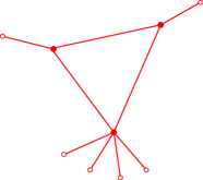
Figure 7: A Feynman graph that cannot be drawn on a loom.

Second, even when the topology of a graph is compatible with obtaining it from the loom, the loom construction implies additional relations between scaling dimensions of the propagators besides those that ensure conformality, i.e. besides the relation that the sum of dimensions at each vertex is $D$. In other words, not all conformal graphs are in the integrable class (see Kazakov:2022dbd for a recent discussion of this). To illustrate the existence of these relations, consider the 3-point graph shown on figure 6. Here in addition to the three constraints coming from the sum of dimensions being $D$ at each vertex,

$$\Delta_{1}+\Delta_{1}^{\prime}+\Delta_{3}^{\prime}=D\ ,\ \ \Delta_{2}+\Delta_{1}^{\prime}+\Delta_{2}^{\prime}=D\ ,\ \ \Delta_{3}+\Delta_{2}^{\prime}+\Delta_{3}^{\prime}=D\ ,\$$ (5)

we have an extra ’non-local’ (i.e. not associated to a single internal vertex) constraint

$$\Delta_{1}^{\prime}+\Delta_{2}^{\prime}+\Delta_{3}^{\prime}=D/2\ .$$ (6)

It follows from expressing the dimensions in terms of the angles $\alpha_{i}$ ($i=1,2,3$) of the grey inner triangle on figure 6 as $\Delta_{i}^{\prime}=D/(2\pi)\alpha_{i}$ and using $\alpha_{1}+\alpha_{2}+\alpha_{3}=\pi$. Conversely, this constraint allows for the application of star-triangle relation to the internal triangle. These extra relations between scaling dimensions are often crucial for ensuring integrability properties such as Yangian symmetry as we will see later on. More involved examples of these non-local constraints are given in section 5.

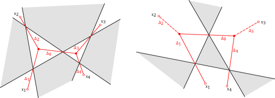
Figure 8: The same Feynman graph drawn on two different looms.

Third, somewhat surprisingly, it can happen that the same Feynman graph can be drawn on two different looms. In both cases the result has Yangian symmetry, but the two constructions can lead to two different sets of constraints on its scaling dimensions. In particular it could happen that one set of constraints is weaker than the other one but is still sufficient for integrability. An example is shown on figure 8. In this case the left figure gives constraints

$$\Delta_{1}+\Delta_{2}+\Delta_{0}=D\ ,\ \ \ \Delta_{3}+\Delta_{4}+\Delta_{0}=D\ ,$$ (7)

while the right one gives an additional constraint

$$\Delta_{1}+\Delta_{0}+\Delta_{4}=D/2\ ,$$ (8)

which follows from considering the angles of the grey triangle in the middle. As the first representation already guarantees Yangian symmetry for the graph, it is clear that this new constraint (8) is in fact not needed for it. Thus in this case one representation provides a strictly weaker set of constraints that ensure integrability. Accordingly, when investigating whether or not a particular graph is in the integrable class one should try to look for different ways to obtain it from the loom. It would be interesting to find an algorithm that provides the minimal set of constraints for a given graph.

Fourth, notice that it could happen that two external legs end inside the same face, see figure 8 (right) for an example. While in general the logic of the construction of Zamolodchikov:1980mb suggests there is only one $x$ variable to be associated with each face, in this case we observed that we do have Yangian symmetry if we keep the external coordinates for these legs distinct (on figure 8 these are $x_{1}\neq x_{4}$). This seems quite natural since in general bringing together coordinates of some external legs is also a potentially dangerous procedure with which the Yangian symmetry may not commute (see e.g. Loebbert:2020tje ; Corcoran:2021gda ).

3 Conformal algebra and Lax operators

We work in the conventions of Chicherin:2012yn and we can take the metric to be either Minkowski,

$$g_{\mu\nu}={\rm diag}(1,-1,-1,\dots,-1)\ ,\ \ \ \ \ \mu,\nu=0,\dots,D-1\ ,$$ (9)

or Euclidean. The conformal algebra generators acting on scalar fields of dimension $\Delta$ have the form

$$P_{\mu}=-i\partial_{x_{\mu}}\equiv\hat{p}_{\mu}\ ,\ \ D=x^{\mu}\hat{p}_{\mu}-i\Delta\ ,$$ (10)

$$L_{\mu\nu}=x_{\nu}\hat{p}_{\mu}-x_{\mu}\hat{p}_{\nu}\equiv\hat{\ell}_{\mu\nu}\ ,\ \ \ K_{\mu}=2x^{\nu}\hat{\ell}_{\nu\mu}+x_{\nu}x^{\nu}\hat{p}_{\mu}-2i\Delta x_{\mu}\ .$$ (11)

We also define

$${\bf x}=-i{\bm{\bar{\sigma}}}^{\mu}x_{\mu}\ ,\ \ \ {\bf p}=-\frac{i}{2}{\bm{\sigma}}^{\mu}\partial_{x_{\mu}}\ ,$$ (12)

using the sigma matrices which in arbitrary even dimension $D$ have size $2^{D/2-1}\times 2^{D/2-1}$ (see Chicherin:2012yn for details).

The Lax operator for the conformal group reads Chicherin:2012yn

$$L_{\alpha\beta}(u_{+},u_{-})=\begin{pmatrix}u_{+}-{\bf p}{\bf x}&{\bf p}\\ {\bf x}(u_{+}-u_{-})-{\bf x}{\bf p}{\bf x}&{\bf x}{\bf p}+u_{-}\end{pmatrix}\ .$$ (13)

It is a matrix of size $2^{D/2}\times 2^{D/2}$ with indices taking values $\alpha,\beta=1,\dots,2^{D/2}$. Here we took the physical space to be the scalar representation with dimension $\Delta$ while the auxiliary space is the $2^{D/2}$-dimensional spinor representation of the conformal group. The parameters $u_{\pm}$ encode the spectral parameter $u$ and the dimension $\Delta$ via

$$u_{+}=u+\frac{\Delta-D}{2}\ ,\ \ u_{-}=u-\frac{\Delta}{2}\ ,$$ (14)

which implies

$$\Delta=u_{+}-u_{-}+D/2\ ,\ \ u=\frac{1}{2}(u_{+}+u_{-}+D/2)\ .$$ (15)

Below we will use shortened notation for the Lax operator with shifted arguments,

$$L[\delta^{+},\delta^{-}]\equiv L[u+\delta^{+},u+\delta^{-}]\ ,$$ (16)

and similarly for a single number

$$[\delta]\equiv u+\delta\ .$$ (17)

The above construction of the Lax operator is formulated for even dimension only. However, its final outcome are differential equations for the graphs discussed in section 5, in which the dimension appears just as a parameter. It is natural to expect that these equations should hold in any dimension (including odd $D$).

3.1 Properties of Lax operators

Below we will extensively use several important properties of this Lax operator. First, we have the key intertwining relation (derived in Chicherin:2012yn , see equation (5.4) there)

$$L_{1}(u+\Delta,u^{\prime})L_{2}(v,u)\frac{1}{x_{12}^{2\Delta}}=\frac{1}{x_{12}^{2\Delta}}L_{1}(u,u^{\prime})L_{2}(v,u+\Delta)\ ,$$ (18)

which allows one to move a propagator through two Lax operators with appropriately chosen arguments. Furthermore, for specially chosen arguments $L$ acts diagonally on a constant function,

$$L_{\alpha\beta}(u,u+D/2)\cdot 1=(u+D/2)\delta_{\alpha\beta}\ ,$$ (19)

as one can verify using identities between sigma matrices given in Chicherin:2012yn . We will also denote by $L^{T}$ the Lax operator obtained from the original one by a ‘transposition’ in the physical space which amounts to integration by parts, i.e. replacing $x^{\mu}\to x^{\mu},\;\partial_{\mu}\to-\partial_{\mu}$ and reversing the order of all $x$ and $\partial_{x}$ operators. In other words, we have

$$\int d^{D}x\;g(x)L_{\alpha\beta}(u,v)f(x)=\int d^{D}x\;(L_{\alpha\beta}^{T}(u,v)g(x))f(x)\ .$$ (20)

Then one can verify that similarly to (19) we have

$$L^{T}_{\alpha\beta}(u+D/2,u)\cdot 1=(u+D/2)\delta_{\alpha\beta}\ .$$ (21)

We will also use the inversion formulas which can be checked by direct computation and generalize those from Chicherin:2017cns to any (even) dimension $D$,

$$L(u_{+},u_{-})^{-1}=-\frac{1}{u_{+}u_{-}}L(-u_{-},-u_{+})\ ,$$ (22)

$$(L(u_{+},u_{-})^{t})^{-1}=-\frac{1}{(u_{+}+D/2)(u_{-}+D/2)}L^{t}(-u_{-}-D,-u_{+}-D)\ ,$$ (23)

where $t$ denotes transposition in the matrix indices.

4 Yangian invariance

In this section we show that the Feynman graphs obtained from the loom construction are Yangian invariants. Namely, they are eigenstates of the monodromy matrix built as a product of $n$ conformal Lax operators (13) where $n$ is the number of external legs of the graph,

$$(L_{n}[\delta_{n}^{+},\delta_{n}^{-}]\dots L_{2}[\delta_{2}^{+},\delta_{2}^{-}]L_{1}[\delta_{1}^{+},\delta_{1}^{-}])_{\alpha\beta}|G\rangle=\delta_{\alpha\beta}\lambda(u)|G\rangle\ .$$ (24)

Here we denoted by $|G\rangle$ the Feynman integral corresponding to the graph, and the Lax operator $L_{k}$ acts on the coordinate $x_{k}$ of the $k$-th external leg of the graph (we used the notation (16) for arguments of Lax operators). Notice that the graph is an eigenstate of all the monodromy matrix elements (not just the trace as usual for spin chains). The shifts $\delta_{k}^{\pm}$ are read off from the geometry of the graph as we describe in detail below.

4.1 Simple example: cross integral with generic dimensions

To illustrate how the construction works let us start with a simple example of a cross integral with generic dimensions $\Delta_{k}$ of the propagators,

$$I=\int\frac{d^{D}x_{0}}{(x_{10})^{2\Delta_{1}}(x_{20})^{2\Delta_{2}}(x_{30})^{2\Delta_{3}}(x_{40})^{2\Delta_{4}}}\ ,$$ (25)

with the constraint

$$\sum_{k=1}^{4}\Delta_{k}=D$$ (26)

that ensures the graph is conformal. When $D=4$ and all dimensions are set to $\Delta_{i}=1$ the result is given by the Bloch-Wigner function,

$$I=\frac{\phi(z,\bar{z})}{x_{13}^{2}x_{24}^{2}}\ ,\ \ \$$ (27)

with

$$z\bar{z}=\frac{x_{12}^{2}x_{34}^{2}}{x_{13}^{2}x_{24}^{2}}\ ,\ \ \ (1-z)(1-\bar{z})=\frac{x_{14}^{2}x_{23}^{2}}{x_{13}^{2}x_{24}^{2}}$$ (28)

and

$$\phi=\frac{\pi^{2}}{z-\bar{z}}(2{\rm Li}_{2}(z)-2{\rm Li}_{2}(\bar{z})+\log\frac{1-z}{1-\bar{z}}\log(z\bar{z}))\ .$$ (29)

For the case of generic $D$ and $\Delta$’s the statement of Yangian invariance is known from Loebbert:2019vcj and the integral itself was found in that work to be a combination of Appell hypergeometric functions Usyukina:1992jd ; Boos:1990rg . Here it will serve as a useful pedagogical example to illustrate the construction. We will show that it’s an eigenstate of the monodromy matrix

$$M \equiv L_{4}[D,\Delta_{1}+\Delta_{2}+\Delta_{3}+D/2]L_{3}[\Delta_{1}+\Delta_{2}+\Delta_{3},\Delta_{1}+\Delta_{2}+D/2]$$

$$\times L_{2}[\Delta_{1}+\Delta_{2},\Delta_{1}+D/2]L_{1}[\Delta_{1},D/2]\ .$$

The derivation closely follows Chicherin:2017cns , extending it to this more general case. The main trick is to use (21) to write

$$1=\frac{1}{[D/2]}L_{0}^{T}[D/2,0]\cdot 1$$ (31)

where we introduced an extra Lax operator associated with $x_{0}$ and acting here on a constant with arguments chosen so that the result is proportional to the identity. We insert (31) under the integral in (25) and integrate by parts which amounts to replacing $L_{0}^{T}$ by $L_{0}$ so we have

$$I = \int d^{D}x_{0}\frac{1}{(x_{10})^{2\Delta_{1}}(x_{20})^{2\Delta_{2}}(x_{30})^{2\Delta_{3}}(x_{40})^{2\Delta_{4}}}\left(\frac{L_{0}^{T}[D/2,0]\cdot 1}{[D/2]}\right)$$

$$= \frac{1}{[D/2]}\int d^{D}x_{0}L_{0}[D/2,0]\frac{1}{(x_{10})^{2\Delta_{1}}(x_{20})^{2\Delta_{2}}(x_{30})^{2\Delta_{3}}(x_{40})^{2\Delta_{4}}}\ .$$

Next we consider the action of the monodromy matrix (4.1) on this integral. The first Lax matrix to act on it is $L_{1}$, in addition to $L_{0}$ which is already present in (4.1). Nicely, we chose the arguments of the Lax matrices in such a way that we can use the intertwining relation (18) to move the first propagator $\frac{1}{(x_{10})^{2\Delta_{1}}}$ through the product $L_{1}L_{0}$, namely

$$L_{1}[\Delta_{1},D/2]L_{0}[D/2,0]\frac{1}{(x_{10})^{2\Delta_{1}}}=\frac{1}{(x_{10})^{2\Delta_{1}}}L_{1}[0,D/2]L_{0}[D/2,\Delta_{1}]\ .$$ (33)

After this, $L_{1}$ now acts on a function which is independent of $x_{1}$ and furthermore its arguments differ by $D/2$, so we can use its action (19) on the identity and we can simply replace it by its eigenvalue which gives a factor $[D/2]$.

At the next step we now have to act with the $L_{2}$ operator. Again we can use the intertwining relation to pull the propagator through it,

$$L_{2}[\Delta_{1}+\Delta_{2},\Delta_{1}+D/2]L_{0}[D/2,\Delta_{1}]\frac{1}{(x_{20})^{2\Delta_{2}}}=\frac{1}{(x_{20})^{2\Delta_{2}}}L_{2}[D/2,\Delta_{1}+D/2]L_{0}[D/2,\Delta_{1}+\Delta_{2}]\ .$$ (34)

As before, we see that in the r.h.s. $L_{2}$ now acts on the constant function and can replaced by its eigenvalue $[\Delta_{1}+D/2]$. Repeating the same steps for $L_{3}$ and $L_{4}$, we see that again we can pull the corresponding propagators through each one of them and in the end these Lax’es are replaced by their eigenvalues. One can see that at the very last step we will be left with action of $L_{0}$ on a constant with the arguments chosen as $L_{0}[D/2,\Delta_{1}+\Delta_{2}+\Delta_{3}+\Delta_{4}]$. Using that the sum of dimensions is $D$ we see that this Lax matrix becomes diagonal as well and just produces an extra scalar factor $[D]$. Collecting all the steps together, we find that the integral is indeed a Yangian invariant,

$$M_{\alpha\beta}I=\lambda(u)\delta_{\alpha\beta}I\ ,$$ (35)

and the eigenvalue reads

$$\lambda(u)=[\Delta_{1}+D/2][\Delta_{1}+\Delta_{2}+D/2][\Delta_{1}+\Delta_{2}+\Delta_{3}+D/2][D]\ .$$ (36)

This simple example illustrates the main idea one can use to prove Yangian invariance for more general graphs. Namely, we insert extra Lax operators at the internal vertices and then use a chain of intertwining relation to gradually get rid of Lax operators acting on parts of the graph. In Chicherin:2017cns this was called the ‘lasso’ method and we found that it extends to the more general graphs we consider here. We give a detailed derivation of how it works in the following subsections.

A key part of the construction is choosing the labels $\delta_{k}^{\pm}$ which ensure the Yangian invariance of the graph. We summarize how this is done in the next subsection.

4.2 Prescription for labels of Lax operators

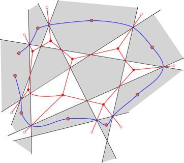
Figure 9: The lasso and the Feynman graph on the loom. The chain of Lax operators is shown in blue, with the orange circles showing contraction of the indices of adjacent Lax operators.

In this section we summarize how one should choose the shifts $\delta^{\pm}_{k}$ in the arguments of the monodromy matrix (24). The reason why this prescription works is described in detail for the cross example in section 4.1. The general arguments will be provided in the next section 4.3. For some cases the prescription was given in Loebbert:2020hxk but the situation we consider is more general.

As a start, for the first external leg with dimension $\Delta$ we choose the labels to be $[\Delta,D/2]$. More generally, the labels of the Lax operator acting on an arbitrary $k$-th external leg will always have the form $[w+\Delta_{k},w+D/2]$ for some $w$ (for the very first leg $w=0$). This ensures that indeed the label $\Delta$ of the representation on which the Lax operator acts, as read off from (15), matches $\Delta_{k}$.

Let us describe how the labels change as we move from leg $k$ to leg $k+1$. First, consider the case when these two legs are attached to the same internal vertex. Denoting by $L_{k}[w+\Delta_{k},w+D/2]$ the Lax operator for the $k$-th leg, we prescribe that the next Lax operator should be chosen as

$$L_{k+1}[w+\Delta_{k}+\Delta_{k+1},w+\Delta_{k}+D/2]\ .$$ (37)

In other words, as we go from leg $k$ to leg $k+1$ we should shift $w\to w+\Delta_{k}$. We illustrate this prescription on figure 10. One can see that this reproduces the labels we used for the cross integral in section 4.1.

Figure 10: Labels for consecutive Lax operators, that share a common vertex. Three of the vertices are depicted with the corresponding Lax operators (37)

Alternatively, it could happen that the next leg is attached to a different vertex. Let us label the internal vertex connected to leg $k$ as $0$, and the one connected to leg $k+1$ as $\tilde{0}$. In the most general situation these two vertices $0$ and $\tilde{0}$ may not even be connected directly. However they will always be linked by a chain of propagators between consecutive internal vertices (see figure 11), starting at vertex $0$ and ending at vertex $\tilde{0}$. Let us label the dimensions of propagators in this chain as $\Delta_{1}^{\prime},\dots,\Delta_{p}^{\prime}$. Then, if the Lax operator for leg $k$ had the form $L_{k}[w+\Delta_{k},w+D/2]$, we find that the one for vertex $k+1$ reads $L_{k+1}[\tilde{w}+\Delta_{k},\tilde{w}+D/2]$ where

$$\tilde{w}=w+\Delta_{k}+\sum_{i=1}^{p}(\Delta_{i}^{\prime}-D/2)\ .$$ (38)

Figure 11: Prescription of labels for the Lax operator in the case when consecutive external legs do not share a common internal vertex. Here $\tilde{w}$ is given by (38) with $p=3$.

For completeness let us also spell out the corresponding terms in the integral:

$$\begin{split}&\ldots L_{k}\left[w+\Delta_{k},w+\dfrac{D}{2}\right]L_{k+1}\left[w+\Delta_{k},w+\dfrac{D}{2}\right]\ldots\times\\ &\qquad\times\int\ldots dx_{k}\prod_{i^{\prime}=1}^{p}dx_{i^{\prime}}dx_{k+1}\ldots\times\\ \qquad&\times\ldots\dfrac{1}{\left(x_{0k}\right)^{2\Delta_{k}}}\dfrac{1}{\left(x_{01}\right)^{2\Delta^{\prime}_{1}}}\left(\prod_{i^{\prime}=2}^{p-1}\dfrac{1}{\left(x_{i^{\prime}(i^{\prime}+1)}\right)^{2\Delta^{\prime}_{i^{\prime}}}}\right)\dfrac{1}{\left(x_{p\,\tilde{0}}\right)^{2\Delta_{p}}}\dfrac{1}{\left(x_{\tilde{0}(k+1)}\right)^{2\Delta_{k+1}}}\ldots\end{split}$$ (39)

Together these rules completely fix the labels one should use to build the monodromy matrix for any graph in the class we consider. To compare this with the $D=4$ fishnet case we notice, that for $\Delta_{k}=1$ and $D=4$ our prescription turns into the one described in Chicherin:2017cns ; Chicherin:2017frs . That is easiest to see for simple graphs with convex corners: when we follow along single external legs the parameters stay constant i.e. $\tilde{w}=w$ in (38). On the other hand, when we encounter a vertex with two external legs at a turn we have $[w+1,w+2]\rightarrow[w+2,w+3]$.

4.3 Moving the lasso

The claim of Yangian invariance relies on the possibility to reduce the Lax chain that constitutes the lasso to the identity operator. This is achieved via a series of applications of the intertwining relations, pulling all the propagators through the Lax chain. This procedure is represented graphically as pulling the lasso through the diagram, resulting in effectively removing it entirely at the end. The graphical representation in the $D=4$ fishnet case is given in Chicherin:2017cns ; Chicherin:2017frs . Here we will generalize the graphical moves to accommodate the diverse graph geometries.

Consider a single boundary vertex which is labelled by the coordinate $x_{0}$. As it lies on the boundary of the diagram, this vertex has neighbouring vertices of two types: external $x^{\mathrm{ext}}_{i}$ and internal $x^{\mathrm{int}}_{j}$. The Lax operators initially act on the external vertices with labels prescribed as in section 4.2. In fact we can flip the lasso in such a way that it will now act on the internal vertices instead, as depicted on figure 12.

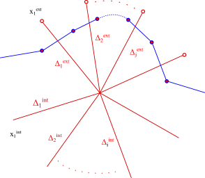
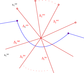
Figure 12: The first transformation rule that describes flipping the lasso from external legs to internal legs. This should be compered with fig. 4 in Chicherin:2017frs and fig. 9 in Chicherin:2017cns .

This transformation generalizes the rules on fig. 4 in Chicherin:2017frs and fig. 9 in Chicherin:2017cns . In particular for the fishnet graph there are two possibilities with either one or two or three external vertices.

Figure 12 is the graphical representation of the following equality:

$$\begin{split}\int d^{D}&x_{0}\left(\prod_{i=1}^{n_{\mathrm{ext}}}L_{i}\left[w+\sum_{k=1}^{i}\Delta^{\mathrm{ext}}_{k},w+\dfrac{D}{2}+\sum_{k=1}^{i-1}\Delta^{\mathrm{ext}}_{k}\right]\right)\cdot\prod_{i=1}^{n_{\mathrm{ext}}}\dfrac{1}{(x^{\mathrm{ext}}_{0i})^{2\Delta^{\mathrm{ext}}_{i}}}\cdot\prod_{j=1}^{n_{\mathrm{int}}}\dfrac{1}{(x^{\mathrm{int}}_{0j})^{2\Delta^{\mathrm{int}}_{j}}}=\\ =&\prod_{i=1}^{n_{\mathrm{ext}}}\left[w+\Delta^{\mathrm{ext}}_{j}+\dfrac{D}{2}\right]\times\\ \times\ \ &\int d^{D}x_{0}\prod_{i=1}^{n_{\mathrm{ext}}}\dfrac{1}{(x^{\mathrm{ext}}_{0i})^{2\Delta^{\mathrm{ext}}_{i}}}\cdot L_{0}\left[w+\dfrac{D}{2},w+\sum_{j=1}^{n_{\mathrm{ext}}}\Delta^{\mathrm{ext}}_{j}\right]\cdot\prod_{j=1}^{n_{\mathrm{int}}}\dfrac{1}{(x^{\mathrm{int}}_{0j})^{2\Delta^{\mathrm{int}}_{j}}}\ .\end{split}$$ (40)

Here $n_{\mathrm{ext}}$ and $n_{\mathrm{int}}$ are the number of external and internal vertices respectively. Thus, the prescription for the parameters of the Lax operator in sec. 4.2 for legs attached to the same vertex is chosen in such a way that formula (40) would works.

On the other hand it is important that the labels between two consecutive sets of external lines are in agreement, which enables the second prescription in section 4.2. Indeed, consider now two vertices $x_{0}$ and $x_{0}^{\prime}$ with external vertices $x_{k}^{\mathrm{ext}}$ and $x_{k^{\prime}}^{\mathrm{ext}}$ and internal vertices $x_{j}^{\mathrm{int}}$ and $x_{j^{\prime}}^{\mathrm{int}}$, drawn on figure 13.

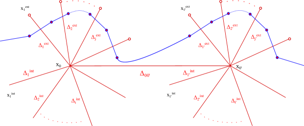
Figure 13: The Lax operator chain for two neighbouring internal vertices $x_{0}$ and $x_{0^{\prime}}$. For simplicity we consider the $p=1$ case of (38).

The Lax parameters for each vertex are as prescribed but with parameters $w$ and $\tilde{w}$ as in section 4.2. Suppose we make the transformation for each vertex (40), which will leave us with the configuration on figure 14.

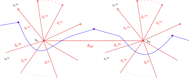
Figure 14: The Lax chain after transformations of fig. 12 was applied to each vertex $x_{0}$ and $x_{0}^{\prime}$. The figure corresponds to the l.h.s of (41)

One of the vertices internal for $x_{0}$ is $x_{0}^{\prime}$ itself and vice versa. Let us look at the propagator connecting those two vertices $x_{00^{\prime}}$ which has dimension $\Delta_{00^{\prime}}$ and consider the intertwining relation:

$$\begin{split}L_{0}&\left[w+\dfrac{D}{2},w+\sum_{j=1}^{n_{\mathrm{ext}}}\Delta^{\mathrm{ext}}_{j}\right]\cdot L_{0^{\prime}}\left[\tilde{w}+\dfrac{D}{2},\tilde{w}+\sum_{j^{\prime}=1}^{n^{\prime}_{\mathrm{ext}}}\Delta^{\mathrm{ext}}_{j^{\prime}}\right]\dfrac{1}{\left(x_{00^{\prime}}\right)^{2\Delta_{00^{\prime}}}}=\\ &=\dfrac{1}{\left(x_{00^{\prime}}\right)^{2\Delta_{00^{\prime}}}}L_{0}\left[\tilde{w}+\sum_{j^{\prime}=1}^{n^{\prime}_{\mathrm{ext}}}\Delta^{\mathrm{ext}}_{j^{\prime}},w+\sum_{j=1}^{n_{\mathrm{ext}}}\Delta^{\mathrm{ext}}_{j}\right]\cdot L_{0^{\prime}}\left[\tilde{w}+\dfrac{D}{2},w+\dfrac{D}{2}\right]\ .\end{split}$$ (41)

In order for this relation to hold we have to set:

$$w+\dfrac{D}{2}=\tilde{w}+\sum_{j^{\prime}=1}^{n^{\prime}_{\mathrm{ext}}}\Delta^{\mathrm{ext}}_{j^{\prime}}+\Delta_{00^{\prime}}$$ (42)

which is nothing but the case $p=1$ of the prescription (38) announced above. By using this relation we will finally have the configuration on figure 15, which means we have pulled the lasso through the $00^{\prime}$ edge.

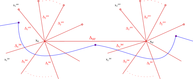
Figure 15: The Lax operator has been pulled of the $00^{\prime}$ edge, as on the r.h.s of (41). To be able to make this transformation we should impose (38)

The fact that the graphical moves actually result in the lasso being completely removed is rather nontrivial. It relies on the prescription of Lax labels being consistent with the dimensions of the external and internal vertices. We prefer to think that there are two types of relations between dimensions that appear. Relations of the first type, which we call local, represent only the fact that the diagram is conformal, i.e. the sum of conformal dimensions adds up to $D$. The second type of relations are in contrast referred to as non-local and are a direct consequence of the Loom construction: since the initial lattice is made up from straight lines there are geometric relations between far separated angles and hence between conformal dimensions. Examples of such relations are discussed in sections 2.2 and 5.1.

Let us now prove that the lasso can be moved past a single vertex completely. To do this, consider the same vertex $x_{0}$. For each line going to an ”internal” vertex consider now its neighbours. For a vertex $x^{\mathrm{int}}_{j}$ we label them by the coordinates $y_{i,j}$. Assume for simplicity that the graph is big enough, such that the lasso does not pass through any of the mentioned edges other than $x_{0i}$. The setup is represented on figure 16. Now first pull the lasso through the $x_{0}$ vertex using (40). We still have the $L_{0}$ Lax operator on the r.h.s. which we want to get rid of, such that the $x_{0}$ coordinate is completely out of the game. To do this first use the conformal nature of the diagram and rewrite the parameters of the Lax operator $L_{0}$ in terms of dimensions of internal legs:

$$L_{0}\left[w+\dfrac{D}{2},w+\sum_{j=1}^{n_{\mathrm{ext}}}\Delta^{\mathrm{ext}}_{j}\right]=L_{0}\left[w+\dfrac{D}{2},w+D-\sum_{j}\Delta^{\mathrm{int}}_{j}\right]\,.$$ (43)

Then use the move on fig. 16 again but for the last (with label $n_{\mathrm{int}}$)internal vertex $x_{n_{\mathrm{int}}}^{\mathrm{int}}$:

$$\begin{split}&\int d^{D}x_{0}d^{D}x_{n_{\mathrm{int}}}^{\mathrm{int}}L_{0}\left[w+\dfrac{D}{2},w+D-\sum_{j=1}^{n_{\mathrm{int}}}\Delta^{\mathrm{int}}_{j}\right]\dfrac{1}{(x_{0n_{\mathrm{int}}}^{\mathrm{int}})^{2\Delta_{n_{\mathrm{int}}}^{\mathrm{int}}}}\cdot\prod_{j=1}^{n_{\mathrm{int}}-1}\dfrac{1}{(x^{\mathrm{int}}_{0j})^{2\Delta^{\mathrm{int}}_{j}}}\times\\ &\times\prod_{i=1}^{n}\dfrac{1}{\left(x^{\mathrm{int}}_{n_{\mathrm{int}}}-y_{i,n_{\mathrm{int}}}\right)^{2\Delta_{j}}}\cdot\ldots=\\[1.0pt] &=\int d^{D}x_{0}d^{D}x_{n_{\mathrm{int}}}^{\mathrm{int}}\dfrac{1}{(x_{0n_{\mathrm{int}}}^{\mathrm{int}})^{2\Delta_{n_{\mathrm{int}}}^{\mathrm{int}}}}\dfrac{1}{\left[\tilde{w}+\dfrac{D}{2}\right]}L_{n_{\mathrm{int}}}\left[\tilde{w}+\dfrac{D}{2}-\Delta_{n_{\mathrm{int}}},\tilde{w}\right]\times\\[1.0pt] &\times L_{0}\left[w+\dfrac{D}{2},w+D-\sum_{j=1}^{n_{\mathrm{int}}}\Delta^{\mathrm{int}}_{j}+{\color[rgb]{0,0,1}\Delta^{\mathrm{int}}_{n_{\mathrm{int}}}}\right]\prod_{j=1}^{n_{\mathrm{int}}-1}\dfrac{1}{(x^{\mathrm{int}}_{0j})^{2\Delta^{\mathrm{int}}_{j}}}\cdot\prod_{i=1}^{n}\dfrac{1}{\left(x^{\mathrm{int}}_{n_{\mathrm{int}}}-y_{i,n_{\mathrm{int}}}\right)^{2\Delta_{j}}}\cdot\ldots\end{split}$$ (44)

Figure 16: The Lax chain of the lasso after transformations of fig. 12 (formula (40)) has been applied to $x_{0}$ and $x_{n_{\mathrm{int}}}^{\mathrm{int}}$, for $n_{\mathrm{int}}=4$. This figure demonstrates (44). As clearly seen from the picture, after applying it to all vertices $x_{j}^{\mathrm{int}}$ the lasso won’t act on the the coordinate $x_{0}$ anymore.

This transformation is represented on figure 16. The parameter $\tilde{w}$ is expressed through $w$ as:

$$\tilde{w}=w+\dfrac{D}{2}-\sum_{j=1}^{n_{\mathrm{int}}-1}\Delta_{j}\ .$$ (45)

The key observation is the shift of parameters in the $L_{0}$ Lax operator highlighted in blue in (44). After the transformation we are left with the same Lax operator $L_{0}$ with the parameters now involving one less internal vertex:

$$w+D-\sum_{j=1}^{n_{\mathrm{int}}}\Delta^{\mathrm{int}}_{j}+{\color[rgb]{0,0,1}\Delta^{\mathrm{int}}_{n_{\mathrm{int}}}}=w+D-\sum_{j=1}^{n_{\mathrm{int}}-1}\Delta^{\mathrm{int}}_{j}\ .$$ (46)

It is clear that the same shift will happen for all internal vertices, if we do the same transformation vertex by vertex. Hence after going through all internal vertices $x_{j}^{\mathrm{int}}$ the resulting Lax operator acts on identity, since all the $x_{0j}$ propagators have been pulled through, with the parameters consistently shifted:

$$L_{0}\left[w+\dfrac{D}{2},w+D-\sum_{k}\Delta^{\mathrm{int}}_{k}+{\color[rgb]{0,0,1}\sum_{j}\Delta^{\mathrm{int}}_{j}}\right]\cdot 1=L_{0}\left[w+\dfrac{D}{2},w+D\right]\cdot 1=\left[w+D\right]\cdot 1\ .$$ (47)

For all the internal vertices $x_{j}^{\mathrm{int}}$ we now are at the previous step, where we have a single Lax operator action on $x_{j}^{\mathrm{int}}$. Notice, that the Lax operators the appear for the internal vertices are with appropriate parameters. For example, for the last vertex as in (44), the Lax operator can be rewritten as:

$$L_{n_{\mathrm{int}}}\left[\tilde{w}+\dfrac{D}{2}-\Delta_{n_{\mathrm{int}}},\tilde{w}\right]=L_{n_{\mathrm{int}}}\left[(\tilde{w}-\Delta_{n_{\mathrm{int}}})+\dfrac{D}{2},(\tilde{w}-\Delta_{n_{\mathrm{int}}})+\Delta_{n_{\mathrm{int}}}\right]\ .$$ (48)

Since the corresponding propagator is now external w.r.t to vertex $x_{n_{\mathrm{int}}}$ we are exactly in the situation as in the r.h.s of formula (40). We then repeat the same transformations to consistently remove the Lax chain from each vertex.

The fact that this sequence of moves indeed leads to the lasso being completely pulled off the diagram is a more involved condition on the conformal dimensions. This is because the process of pulling of a single vertex or even between two adjacent vertices requires only the conformal condition and peculiar relations between Lax parameters. These other ones should be the conditions that make the moves on different vertices in distant parts of the diagram consistent with each other. The origin of these relations seems to be the fact that the diagram is drawn on the dual space to the loom – a lattice made up from straight lines.

As a final remark, we expect that the steps we have proven above should also be valid for the generalised case when internal vertices are placed inside open faces as described in section 2.1 and we have checked this for a number of examples. This is also natural as likely the introduction of these vertices may be viewed as a kind of analytic continuation in the space of parameters (i.e. from the case when the face is closed to the case when it is open). We leave details of the proof for this case to the future.

4.4 Cyclicity and computation of the eigenvalue

Using the lasso procedure described above, one can compute the eigenvalue of the monodromy matrix directly for any particular graph. Alternatively, one can in fact write down a difference equation which fixes the eigenvalue in terms of the labels $\delta_{n}^{\pm}$ of the Lax operators. This can be done following Chicherin:2017cns by making use of the properties (22), (23) which ultimately allow one to cyclically reorder the Lax operators inside the monodromy matrix while at the same time shifting their labels $\delta_{n}^{\pm}$ by some constants. The derivation is an immediate generalisation of the discussion from appendix A of Chicherin:2017cns (with minimal modifications due to the $D$-dependent shifts in (22), (23)). As a result, we find that the eigenvalue $\lambda(u)$ satisfies the relation

$$\frac{\lambda(u)}{\lambda(u-D)}=\frac{P(u)}{P(u-D/2)}\ ,$$ (49)

where $P$ is a polynomial encoding the values of $\delta_{n}^{\pm}$,

$$P(u)=\prod_{j=1}^{n}(u+\delta_{j}^{+})(u+\delta_{j}^{-})\ .$$ (50)

This equation completely fixes the eigenvalue $\lambda$. In particular, one can use it to find its large $u$ expansion which will be useful in section 5. We find

$$\lambda(u)=u^{n}+\frac{1}{2}u^{n-1}\sum_{k=1}^{n}\hat{\delta}_{k}+\frac{1}{4}u^{n-2}\left[\sum_{i<j}\hat{\delta}_{i}\hat{\delta}_{j}-\frac{1}{2}\sum_{i}\hat{\Delta}_{i}\right]+\dots$$ (51)

where we denoted (following Chicherin:2017cns )

$$\hat{\delta}_{k}=\delta_{k}^{+}+\delta_{k}^{-}+D/2\ ,\ \ \hat{\Delta}_{i}=\Delta_{i}(\Delta_{i}-D)\ .$$ (52)

We recall that $\Delta_{k}=\delta_{k}^{+}-\delta_{k}^{-}+D/2$.

5 Differential equations from Yangian symmetry and examples

In this section we derive differential equations following from Yangian symmetry and demonstrate them for several examples.

In general the Yangian of a Lie algebra (in our case, the Lie algebra of the conformal group in $D$ dimensions) can be described in terms of level-0 generators $J^{A}$ and level-1 generators ${\widehat{J}}^{A}$, see e.g. Chicherin:2017cns for a more detailed discussion. This is known as the first realization of the Yangian. The level-0 generators are those of the original Lie algebra and satisfy the commutation relations

$$[J^{A},J^{B}]=f^{AB}_{\ \ \ \ C}J^{C}$$ (53)

where $f^{AB}_{\ \ \ \ C}$ are the structure constants. In our case these generators are given by a sum of individual operators acting on each external leg of the graph,

$$J^{A}=\sum_{k=1}^{n}J^{A}_{k}\ .$$ (54)

The level-1 generators are bilocal and can be written as

$$\hat{J}^{A}=\frac{1}{2}f^{A}_{\ \ \ BC}\sum_{j<k}J^{C}_{j}J^{B}_{k}+\sum_{k}v_{k}J^{A}_{k}$$ (55)

in terms of some evaluation parameters $v_{k}$. All other generators of the infinite-dimensional Yangian algebra can be obtained as some polynomial combinations of $J^{A}$ and ${\widehat{J}}^{A}$.

In our case the explicit form of the Yangian generators that annihilate our graph, together with the evaluation parameters $v_{k}$, can be read off from the first few orders of the large $u$ expansion of the monodromy matrix (24) and the eigenvalue $\lambda(u)$. The latter can be obtained from (49) while the former can be found by using the explicit form of the Lax matrix (13). A detailed derivation is given in section 8.3 of Chicherin:2017cns . Extending it to our case with generic dimension $D$, we find that the evaluation parameters are given in terms of the shifts in Lax operators in (24) as

$$v_{k}=\frac{1}{2}\sum_{j\neq k}(\delta_{j}^{+}+\delta_{j}^{-}+D/2)\ .$$ (56)

The conformal generators $J^{A}$ and the level-1 Yangian generators ${\widehat{J}}^{A}$ both annihilate our Feynman integral. While the first statement amounts to conformal invariance of the graph, the second one gives further nontrivial constraints. As discussed in Chicherin:2017cns it is sufficient to consider only the case of the momentum generators, i.e. ${\widehat{J}}^{A}={\widehat{P}}^{\mu}$ (the other generators do not give new independent equations). Explicitly, this generator reads Chicherin:2017cns

$${\widehat{P}}^{\mu}=-\frac{i}{2}\sum_{j<k}[(L_{j}^{\mu\nu}+g^{\mu\nu}D_{j})P_{k,\nu}-(j\leftrightarrow k)]+\sum_{j}v_{j}P_{j}^{\mu}$$ (57)

where the most nontrivial graph-dependent part is the last term. Plugging in the conformal generators from (10), (11) one can write it as an explicit differential operator that annihilates our graph,

$${\widehat{P}}^{\mu}|\rm graph\rangle=0\ .$$ (58)

Let us mention that in (55) we can shift all $v_{k}$ by the same value $v_{k}\to v_{k}+c$ since the level-0 generators $J^{A}$ annihilate our state. For example, by doing this we can always set $v_{1}=0$.

Although the derivation of the differential equations following from Yangian symmetry relies on the explicit form of the Lax matrix (13) which we discussed only for even dimension $D$, the only dependence on $D$ in the end is parametric, contained in the labels $\delta_{k}^{\pm}$ and various shifts proportional to $D$ such as in (56). This suggests that the resulting differential equations in fact hold in any dimension, though it would be important to establish this more rigorously.

Since the graphs are conformal, they must evaluate to some nontrivial functions of the conformal cross-ratios times explicit spacetime dependent prefactors. Plugging this representation into the differential equations, one can separate the terms with different coordinate dependence and obtain differential equations on the independent components written now only in terms of the cross ratios. This rewriting applies to our general case as well and we refer to Loebbert:2022nfu for more details.

As a result, we see that in order to write the differential equations for the graph we simply read off the labels $\delta_{k}^{\pm}$ and plug them into (56), (57). Below we illustrate this on several examples.

5.1 Example: square with 6 legs

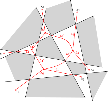
Figure 17: Square with 6 legs.

As a first example, let us consider a graph that looks like a square with 6 external legs (figure 17). It is parameterised by 10 scaling dimensions, labelled as $\Delta_{1},\dots,\Delta_{6}$ and $\Delta_{1}^{\prime},\dots,\Delta_{4}^{\prime}$ on the figure. Imposing that the dimensions at each vertex sum up to $D$ gives four independent relations. In addition to them we have a further ’nonlocal’ relation

$$\Delta_{6}+\Delta_{2}+\Delta_{5}=D$$ (59)

which one can deduce from the geometry and the rule (2) linking dimensions to angles. One can show that this exhausts all independent relations between the dimensions coming from the loom construction in this case. Notice that from these relations it also follows that we have a relation similar to (59),

$$\Delta_{4}+\Delta_{1}+\Delta_{3}=D\ ,$$ (60)

as well as

$$\sum_{i=1}^{4}\Delta_{i}^{\prime}=D\ .$$ (61)

As a result, we can express all 10 dimensions in terms of 5 parameters, for example in terms of $\Delta_{1},\Delta_{2},\Delta_{3},\Delta_{5}$ and $\Delta_{1}^{\prime}$ which gives

$$\Delta_{6}=D-\Delta_{2}-\Delta_{5}\ ,\ \ \ \Delta_{4}=D-\Delta_{1}-\Delta_{3}\ ,$$ (62)

$$\Delta_{2}^{\prime}=D-\Delta_{1}^{\prime}-\Delta_{2}\ ,\ \Delta_{3}^{\prime}=-D+\Delta_{1}+\Delta_{1}^{\prime}+\Delta_{2}\ ,\ \Delta_{4}^{\prime}=D-\Delta_{1}-\Delta_{1}^{\prime}\ .$$ (63)

Using the results of section 4, we can write explicitly the labels for the monodromy matrix of which the graph is an eigenstate. It has the form

$$L_{6}[\Delta_{(11^{\prime})}+D/2,\Delta_{(121^{\prime}5)}]L_{5}[\Delta_{(121^{\prime}5)}-D/2,\Delta_{(121^{\prime})}]L_{4}[D,\Delta_{(13)}+D/2]\times$$ (64)

$$L_{3}[\Delta_{(13)},\Delta_{1}+D/2]L_{2}[\Delta_{(121^{\prime})}-D/2,\Delta_{(11^{\prime})}]L_{1}[\Delta_{1},D/2]$$

where we used the notation

$$\Delta_{(a_{1}a_{2}\dots a_{p})}=\Delta_{a_{1}}+\Delta_{a_{2}}+\dots+\Delta_{a_{p}}\ .$$ (65)

The corresponding evaluation parameters entering the differential equation that follows from Yangian symmetry are obtained from (56) (we used the freedom of shifting them all by the same constant to set $v_{1}=0$),

$$v_{k}=\left\{0,-\Delta_{1}^{\prime}-\frac{\Delta_{1}}{2}-\frac{\Delta_{2}}{2}+D/2,-\frac{\Delta_{1}}{2}-\frac{\Delta_{3}}{2},-\frac{\Delta_{3}}{2}-D/2,\right.$$ (66)

$$\left.\ \ \ \ \ \ \ \ -\Delta_{1}^{\prime}-\frac{\Delta_{1}}{2}-\Delta_{2}-\frac{\Delta_{5}}{2}+D/2,-\Delta_{1}^{\prime}-\frac{\Delta_{1}}{2}-\frac{\Delta_{2}}{2}-\frac{\Delta_{5}}{2}\right\}\ .$$

5.1.1 Reduction to 4 legs

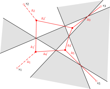
Figure 18: Square with 4 legs.

An interesting limit for this graph with 6 legs is when we set to zero the dimensions $\Delta_{6}$ and $\Delta_{4}$, leaving a graph with only one leg coming out of each vertex. At the level of the relations between scaling dimensions (62), (63) and of the monodromy matrix (64) this is a completely smooth limit. However, limits of this kind often change the configuration of lines of the Baxter lattice in a radical way, and in fact in our case we found that the resulting graph cannot be drawn at all on a conventional loom. However, it can be drawn once we allow the generalisation discussed in section 2.1 when we can place internal vertices inside open faces. This gives the square graph shown earlier on figure 5, and on figure 18 we have added the labels for $\Delta$’s corresponding to our notation here.

From (62) we see that a convenient choice is to set two of the parameters to be

$$\Delta_{5}=D-\Delta_{2}\ ,\ \ \ \Delta_{3}=D-\Delta_{1}$$ (67)

which gives $\Delta_{6}=\Delta_{4}=0$. Then we are left with three independent parameters $\Delta_{1},\Delta_{2},\Delta_{1^{\prime}}$ through which the remaining dimensions are still expressed by (63). Notice that (67) are again examples of nonlocal relations between the dimensions for our graph, as they do not follow from just demanding the sum of dimensions at each vertex to be $D$.

We can smoothly implement the limit $\Delta_{4},\Delta_{6}\to 0$ directly for the monodromy matrix (64) of the original 6-point graph. We notice that the labels of Lax operators $L_{4}$ and $L_{6}$, which correspond to legs we have removed, become such that they are immediately diagonalised due to (19) (explicitly, they become $L_{6}[\Delta_{(11^{\prime})}+D/2,\Delta_{(11^{\prime})}+D]$ and $L_{4}[D,3D/2]$). Therefore they can be simply removed from the monodromy matrix and we are left with a monodromy matrix acting now only on the four legs of our graph. It has the form

$$L_{5}[\Delta_{(11^{\prime})}+D/2,\Delta_{(121^{\prime})}]L_{3}[D,\Delta_{1}+D/2]L_{2}[\Delta_{(121^{\prime})}-D/2,\Delta_{(11^{\prime})}]L_{1}[\Delta_{1},D/2]\ .$$ (68)

Then we find the evaluation parameters to be (setting $v_{1}=0$ )

$$v_{k}=\left\{0,-\Delta_{1}^{\prime}-\frac{\Delta_{1}}{2}-\frac{\Delta_{2}}{2}+D/2,-D/2,-\Delta_{1}^{\prime}-\frac{\Delta_{1}}{2}-\frac{\Delta_{2}}{2}\right\}\ .$$ (69)

Plugging them into (56), (57) gives the differential equation satisifed by this graph. Let us mention that this graph (albeit with some propagators being massive) was partially discussed in Loebbert:2020hxk and now we are able to provide a clear criterion for its Yangian invariance in the massless case, namely the relations (67), (63) between the scaling dimensions.

Let us finally also mention that both for the square with 4 legs and the one with 6 legs we have checked Yangian invariance explicitly by repeated application of the intertwining relation and other properties of the Lax operators, serving as a nontrivial test of the general procedure for removing the lasso that we described in section 4.

6 Yangian invariance with infinite-dimensional auxiliary space

In this section we show that the Feynman graphs we discuss are also invariant under the action of the monodromy matrix that has an infinite-dimensional auxiliary space. That is, we take the auxiliary space to be a representation of the same type as the physical one, labelled by a scaling dimension $\Delta_{a}$ which is now an extra parameter in the construction. This representation cannot be obtained by fusion from finite-dimensional representations and thus its application to the Yangian symmetry potentially provides new and potentially powerful constraints on Feynman graphs. While the case we discussed above led to differential equations for the graphs, here we will get integral equations as the corresponding R-matrix is now an integral operator. Let us notice that this construction is new even for the simplest $D=4$ fishnet with a quartic interaction and it would be interesting to explore its implications. At the same time, those new Yangian integral equations represent new relations establishing equivalence between very different Feynman diagrams.

Figure 19: The kernel of the R-matrix as an integral operator. The physical space corresponds to the vertical direction and the auxiliary space to the horizontal direction.

The conformal R-matrix for the case we are discussing was constructed in Chicherin:2012yn . Let us label the physical and auxiliary spaces as ’$1$’ and ’$a$’ respectively, with the corresponding scaling dimensions

$$\Delta_{1}=\Delta_{phys}\ ,\ \Delta_{a}=\Delta_{aux}\ .$$ (70)

The tensor product of these two spaces corresponds to the space of functions $f(x_{1},x_{a})$. Then the kernel of the R-matrix is given on figure 19 and it acts on a function as

$$(R_{1a}f)(x_{1},x_{a})=4^{2(u-v)}A(-(u-v)-\rho)A(-(u-v)+\rho)\int\frac{d^{D}y_{1}d^{D}y_{a}\;f(y_{1},y_{a})}{x_{1a}^{2\alpha_{+}}(x_{1}-y_{a})^{2\beta_{+}}(x_{a}-y_{1})^{2\beta_{-}}y_{1a}^{2\alpha_{-}}}\ ,$$ (71)

where we denoted

$$\alpha_{+}=v_{+}-u_{-}\ ,\ \alpha_{-}=v_{-}-u_{+}\ ,\ \beta_{-}=u_{+}-v_{+}+D/2\ ,\ \beta_{+}=u_{-}-v_{-}+D/2$$ (72)

and

$$u_{+}=u+\frac{\Delta_{a}-D}{2}\ ,\ u_{-}=u-\frac{\Delta_{a}}{2}\ ,\ v_{+}=v+\frac{\Delta_{1}-D}{2}\ ,\ v_{-}=v-\frac{\Delta_{1}}{2}\ .$$ (73)

We also introduced

$$\rho=\frac{\Delta_{1}-\Delta_{a}}{2}$$ (74)

and

$$A(u)=\frac{\Gamma(D/2-u)}{\Gamma(u)}\ .$$ (75)

In our notation the first space is the physical one (vertical direction on the figure) and the second one is auxiliary (horizontal direction).

Notice that we have four labels $\alpha_{\pm},\beta_{\pm}$ but the R-matrix actually depends only on three parameters: $\Delta_{1},\Delta_{a}$ and the spectral parameter $u-v$. However the labels defined in (72) automatically satisfy an additional constraint

$$\alpha_{+}+\beta_{+}+\alpha_{-}+\beta_{-}=D$$ (76)

ensuring the matching of the number of parameters. Notice also that the individual labels, unlike the final R-matrix, depend separately on $u$ and $v$ so the notation is somewhat redundant.

6.1 Chain and cross relations

Below we will make use of several important identities which allow us to transform expressions built from these R-matrices. First, we will use the chain relation which reads

$$\int d^{D}z\frac{1}{(x-z)^{2\alpha}(z-y)^{2\beta}}=\frac{\pi^{D/2}A(\alpha)A(\beta)A(D-\alpha-\beta)}{(x-y)^{2(\alpha+\beta-D/2)}}\ .$$ (77)

One can also derive from it a representation of the delta-function in terms of a propagator,

$$\lim_{\epsilon\to 0}\frac{\epsilon}{(x-y)^{2(D/2-\epsilon)}}=\frac{\pi^{D/2}}{\Gamma(D/2)}\delta(x-y)\ .$$ (78)

Second, we will use the cross relation shown on figure 20 which is a consequence of the star-triangle identity and allows us to move a propagator through a quartic integration point. It reads

$$\int\frac{d^{D}z}{|x_{1}-z|^{2(D/2-\alpha^{\prime})}|x_{2}-z|^{2\alpha}|y_{1}-z|^{2(D/2-\beta^{\prime})}|y_{2}-z|^{2\beta}}$$ (79)

$$=\int\frac{d^{D}z}{|x_{1}-z|^{2\alpha^{\prime}}|x_{2}-z|^{2(D/2-\alpha)}|y_{1}-z|^{2\beta^{\prime}}|y_{2}-z|^{2(D/2-\beta)}}$$

$$\ \ \ \times A(\alpha)A(\beta)A(D/2-\alpha^{\prime})A(D/2-\beta^{\prime})$$

and is satisfied as long as

$$\alpha+\alpha^{\prime}=\beta+\beta^{\prime}\ .$$ (80)

Figure 20: The cross relation which holds for $\alpha+\alpha^{\prime}=\beta+\beta^{\prime}$.

6.2 Properties of the R-matrix

Our main idea is to show that analogs of the key properties (18), (19), (21) of the Lax operator with finite-dimensional auxiliary space we used above have direct analogs for the infinite-dimensional case, i.e. for the R-matrix (71). After that the whole lasso construction from section 4 can be used without changes and will ensure the invariance of the Feynman graphs.

6.2.1 Intertwining relation

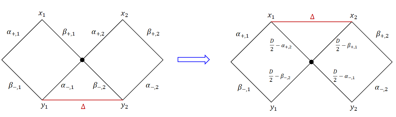
Figure 21: Moving the propagator through two R-matrices.

The first key property we will need is an analog of the intertwining relation (18) which allows one to move a propagator through a product of two R-matrices. Remarkably it also extends to our case and can be derived using the cross relation (79). Concretely, let us consider two R-matrices $R_{1a}$ and $R_{2a}$, with $R_{ka}$ acting on the $k$-th physical space and in the auxiliary space. We will introduce the following convenient notation for the R-matrices. First, denote by $R(u_{+},u_{-},v_{+},v_{-})$ the R-matrix defined as above by (71) with conventions (72), (73). To write the intertwining relation in a way similar to the finite-dimensional case (18), let us introduce the operator

$$L^{\rm inf}_{k}(w_{+},w_{-})=R_{ka}((\Delta_{a}-D)/2,-\Delta_{a}/2,-D/2-w_{-},-D/2-w_{+})$$ (81)

which acts in the tensor product of the $k$-th physical space and the auxiliary space. Here the arguments are chosen in such a way that the scaling dimension for the auxiliary space is $\Delta_{a}$ while the two parameters $w_{\pm}$ are related to the R-matrix spectral parameter $u-v\equiv u_{R}$ and the scaling dimension in the physical space by exactly the same relations (15) as in the finite-dimensional case, namely

$$u_{R}=\frac{1}{2}(w_{+}+w_{-}+D/2)\ ,\ \ \Delta_{phys}=w_{+}-w_{-}+D/2\ .$$ (82)

The intertwining relation then takes the form

$$L^{\rm inf}_{1}(z+\Delta,w)L^{\rm inf}_{2}(w^{\prime},z)x_{12}^{-2\Delta}=F(z,\Delta,\Delta_{a})x_{12}^{-2\Delta}L^{\rm inf}_{1}(z,w)L^{\rm inf}_{2}(w^{\prime},z+\Delta)$$ (83)

where

$$F(z,\Delta,\Delta_{a})=A\left(-\Delta-\frac{\Delta_{a}}{2}-z\right)A\left(D+\Delta-\frac{\Delta_{a}}{2}+z\right)A\left(-\frac{D}{2}+\frac{\Delta_{a}}{2}-z\right)A\left(\frac{D}{2}+\frac{\Delta_{a}}{2}+z\right)\ .$$ (84)

In order to derive it, one considers the lhs shown graphically on figure 21 and uses the cross relation (79) to move the propagator (shown in red) through the quartic integration point in the middle. This leads to a change of powers of the various propagators, and one also needs to ensure that the cross relation can be applied at all (i.e. the condition (80) is satisfied). Taking all this into account and keeping careful track of the notation, we find as result of a somewhat tedious calculation that we get the simple relation (83). Notice that, in particular, applicability of the cross relation restricts both R-matrices to be constructed with the same value of the scaling dimension $\Delta_{a}$ for the auxiliary space. We can see, in the notation we have chosen, that this relation has exactly the same form as its counterpart (18) for the finite-dimensional case!

6.2.2 Diagonal action on constants

The second key property we will use is an analog of (19) and (21), i.e. a simple action on constant functions when the Lax operator arguments are adjusted in a special way corresponding to $\Delta_{1}=0$ or $\Delta_{1}=D$. Consider first the action of $R_{1a}$ on a function $f=f(x_{a})$ (independent of $x_{1}$) when $\Delta_{1}\to 0$. It gives, using the chain relation for $y_{1}$ integration and then using (78),

$$(R_{1a}f)= \pi^{D/2}4^{2(u-v)}A(-(u-v)-\rho)A(-(u-v)+\rho)A(\alpha_{-})A(\beta_{-})\times$$

$$\frac{\Gamma(D/2-\Delta_{1})}{\Gamma(\Delta_{1})}\frac{1}{x_{1a}^{2\alpha_{+}}}\int\frac{d^{D}y_{a}\;f(y_{a})}{(x_{1}-y_{a})^{2\beta_{+}}(x_{a}-y_{a})^{2(D/2-\Delta_{1})}}$$

$$= \pi^{D}4^{2(u-v)}A(-(u-v)+\Delta_{a}/2)A(-(u-v)-\Delta_{a}/2+D/2)f(x_{a})\ .$$

To write this in a way that looks similar to the finite-dimensional case (19), let us take $f$ to be a delta-function $\delta(x-y)$, then we can use $x,y$ as an analog of the matrix indices in (19). Then using also the notation (81) we find

$$L^{\rm inf}(u,u+D/2)_{xy}\cdot 1=G(u,\Delta_{a})\delta(x-y)$$ (86)

where we defined

$$G(u,\Delta_{a})=(4\pi)^{D}4^{2u}A(-u-D/2+\Delta_{a}/2)A(-u-\Delta_{a}/2)\ .$$ (87)

This relation looks exactly like (19) up to the prefactor $G$.

Furthermore, as before we will also use the R-matrix ’transposed’ in the physical space, defined by the property (schematically)

$$\int dxf(x)(Rg(x))=\int dx(R^{T}f(x))g(x)\ .$$ (88)

Its kernel is obtained from the original one in (71) by simply exchanging $x_{1}\leftrightarrow y_{1}$. Similarly to the finite-dimensional case, here we find for it

$$L^{\rm inf,T}(u+D/2,u)_{xy}\cdot 1=G(u,\Delta_{a})\delta(x-y)\ .$$ (89)

The two properties (86) and (89) are direct analogs of the ones we had for the finite-dimensional case ((19), (21)) and in the notation we have chosen they are nicely written in the same way.

6.3 Monodromy matrix and examples

Above we have shown that direct counterparts of relations (18), (19), (21) we had for the finite-dimensional case exist as well for the R-matrices with infinite-dimensional auxiliary space in the form (83), (86), (89). This means that the whole lasso construction from section 4 goes through and leads to invariance of Feynman graphs under the action of the monodromy matrix constructed as

$$M_{xy}=(L_{n}^{\rm inf}(u+\delta_{n}^{+},u+\delta_{n}^{-})\dots L_{1}^{\rm inf}(u+\delta_{1}^{+},u+\delta_{1}^{-}))_{xy}$$ (90)

where $n$ is the number of external legs of the graph and the labels $\delta_{k}^{\pm}$ are chosen according to the same rules as discussed in section 4. Thus we have

$$M_{xy}|{\rm graph}\rangle=\lambda(u)\delta(x-y)|{\rm graph}\rangle$$ (91)

where the eigenvalue $\lambda(u)$ can be found by applying step by step the procedure of removing the lasso from the diagram discussed in section 4. In practice when computing the eigenvalue one should pay attention to the extra factors $F$ and $G$ in the intertwining relation (83) and the diagonal action (86), (89) that were not present or very simple in the original construction. Notice also several nontrivial differences here compared to the finite-dimensional case:

• The invariance condition for the Feynman graph is now an integral rather than a differential equation

• Since the R-matrices are built out of propagators, the lhs of the eigenvalue equation (91) is itself a Feynman graph, thus this equation can be viewed as a relation between two different Feynman graphs.

• Instead of discrete indices $\alpha,\beta$ in (24) here we have continuous labels $x,y$

• We have an extra parameter in the monodromy matrix, namely the scaling dimension $\Delta_{a}$ associated to the auxiliary space

All these features look rather intriguing and we hope they should lead to new constraints for Feynman graphs. While we postpone a more detailed investigation of the construction to the future, below we will illustrate it on the example of the cross and double cross integrals.

6.3.1 Example: cross integral

Let us first consider the 4-point cross integral (25). For simplicity let us focus on the case when the dimension $D$ is arbitrary but all four propagator scaling dimensions are set to $D/4$. Then repeating the steps from section 4.1, we find that the monodromy matrix in this case is

$$M=L_{4}^{\rm inf}[D,5D/4]L_{3}^{\rm inf}[3D/4,D]L_{2}^{\rm inf}[D/2,3D/4]L_{1}^{\rm inf}[D/4,D/2]$$ (92)

where we used the notation

$$L_{k}^{\rm inf}[\delta^{+},\delta^{-}]=L_{k}^{\rm inf}(u+\delta^{+},u+\delta^{-})\ .$$ (93)

We show the action of the monodromy matrix on the graph on figure 22.

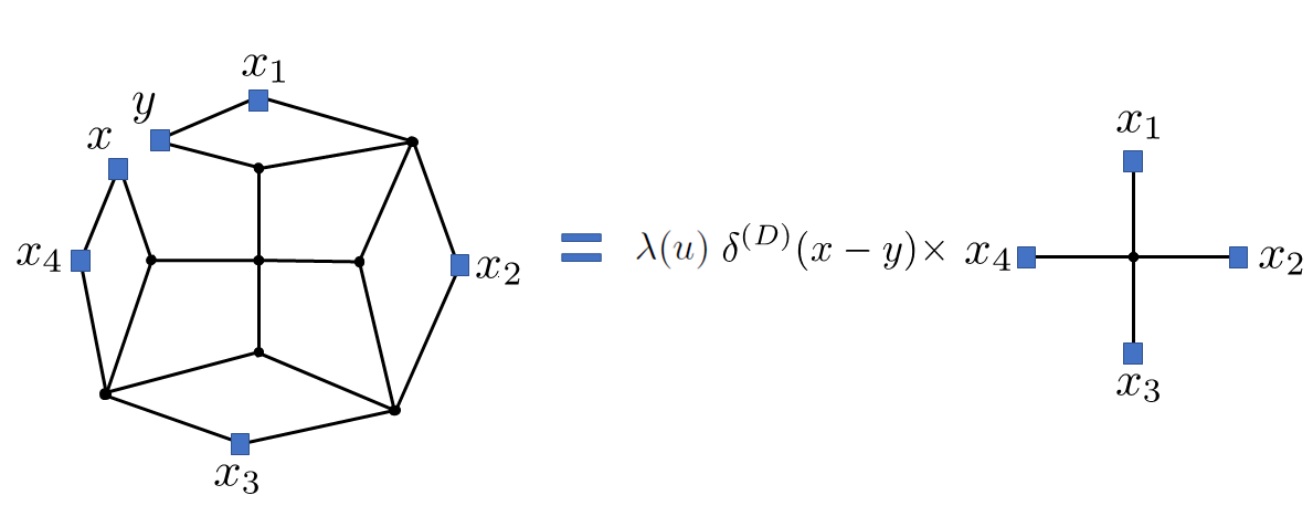
Figure 22: Action on the cross integral of the Yangian monodromy matrix built from $R$-matrices with non-compact representation in auxiliary space. The cross integral is an eigenfunction of this monodromy matrix.

In order to compute the eigenvalue, like before we introduce an extra operator $L_{0}^{{\rm inf},T}$ acting on the integration coordinate $x_{0}$ and then move the propagators one by one through the L-operators, repeating the steps in section 4.1. We give a schematic representation of this process on figure 23.

Figure 23: We remove the parts of the ’lasso’ acting on the cross integral one by one. As a result we find that the integral is an eigenstate of the monodromy matrix. At the first step, we insert an extra $L_{0}$ (drawn in red) using the identity (89), then we apply the cross relation (figure 20) to move outside the propagator coming out of the point $x_{0}$ vertically, which leads to the 2nd configuration; applying the chain relation to the point where only two propagators meet, then the cross relation moving outside the right propagator stemming from the point $x_{0}$ and again the identities (86), we come to the 3rd configuration, etc. At the last step, we apply two chain relations and, again due to (86), we restore the original cross graph, thus proving the Yangian invariance equation for it.

Collecting all the $F$ and $G$ factors originating from (83), (86) we find that the eigenvalue reads

$$\lambda(u)=F(u)G\left(u+\frac{D}{2}\right)\prod_{k=1}^{3}F\left(u+\frac{kD}{4}\right)G\left(u+\frac{kD}{4}\right)$$ (94)

where $F$ and $G$ correspond to the definitions (84), (87) with $\Delta=D/4$ and $\Delta_{a}$ kept arbitrary. For the case when $D=4$ (with $\Delta=1$) this can be simplified to

$$\lambda(u)= \frac{\left(-\frac{\Delta_{a}}{2}+u+4\right)\left(-\frac{\Delta_{a}}{2}+u+5\right){}^{2}\left(\frac{\Delta_{a}}{2}+u+1\right)\left(\frac{\Delta_{a}}{2}+u+2\right)\left(\frac{\Delta_{a}}{2}+u+5\right)}{\left(-\frac{\Delta_{2}}{2}+u+3\right)\left(-\frac{\Delta_{a}}{2}+u+6\right)\left(-\frac{\Delta_{a}}{2}+u+7\right)\left(\frac{\Delta_{a}}{2}+u+3\right){}^{2}\left(\frac{\Delta_{a}}{2}+u+4\right)}$$ (95)

$$\times\pi^{16}4^{8u+32}\left(\frac{A(\Delta_{a}/2-u-3)}{A(\Delta_{a}/2+u+5)}\right)^{4}\ .$$

6.3.2 Example: double cross integral

As another example, consider the more involved 6-point double cross integral, shown on figure 24. Again we will for simplicity take all propagator scaling dimensions to be $D/4$ (generalization to the generic case is straightforward). Then we find that the monodromy matrix whose eigenstate it is has the form

$$L_{6}^{\rm inf}[D,5D/4]L_{5}^{\rm inf}[3D/4,D]L_{4}^{\rm inf}[3D/4,D]L_{3}^{\rm inf}[D/2,3D/4]L_{2}^{\rm inf}[D/4,D/2]L_{1}^{\rm inf}[D/4,D/2]\ .$$ (96)

To compute the eigenvalue we again introduce two new operators $L_{0}^{\rm inf}$ and $L_{0^{\prime}}^{\rm inf}$ at the two integration points and commute the propagators through all the L-operators, via a calculation similar to the one discussed for the double cross (for the usual fishnet theory and usual Lax operators with 4d auxiliary space) in Chicherin:2017cns . In the end we find the eigenvalue to be (in the same notation as in (94))

$$\lambda(u)=F(u)^{2}G\left(u+\frac{D}{2}\right)\prod_{k=1}^{3}\left[F\left(u+\frac{kD}{4}\right)G\left(u+\frac{kD}{4}\right)\right]^{2-\delta_{k,3}}\ .$$ (97)

Figure 24: The double cross integral.

The conformal double cross integral has been computed with generic dimensions but has a highly complicated form with 9-fold nested sums Loebbert:2019vcj ; Ananthanarayan:2020ncn . It would be interesting to see if the constraints coming from our integral Yangian invariance equation could help to simplify it.

7 Conclusions

In this work we derived new Yangian symmetry relations for integrable conformal planar Feynman graphs with disc topology, introduced by A. Zamolodchikov Zamolodchikov:1980mb . Such graphs are ubiquitous for single trace correlators in generalized fishnet CFTs Kazakov:2022dbd in the planar ’t Hooft limit. Our Yangian relations generalize those found in Chicherin:2017cns ; Chicherin:2017frs for particular case of graphs with regular square lattice structure, and then in Loebbert:2019vcj ; Loebbert:2020hxk ; Loebbert:2020tje ; Loebbert:2020glj ; Corcoran:2020epz ; Corcoran:2021gda for specific other cases, to the whole variety of such integrable graphs described in Zamolodchikov:1980mb . The integrablity of these graphs was established in Zamolodchikov:1980mb via the star-triangle relations. Our Yangian relations represent another manifestation of this integrability: the graph turns out to be an eigenfunction of the ‘lasso operator’ acting on its external legs. This lasso operator is a monodromy matrix built out of Lax operators with the spectral parameter changing according to the weights of external propagators. Its auxiliary space could be, a priori, in any representation of the underlying algebra. We consider here, apart from the standard compact representation, also the non-compact principal series representation of $D$-dimensional conformal algebra. Interestingly, this seems to produce some new relations connecting various conformal Feynman graphs as well as new integral equations for the graphs.

Let us point out a few future directions:

• Using our new integral and differential equations it would be interesting to try to bootstrap various new Feynman integrals, extending the Yangian bootstrap program that has already brought novel results Loebbert:2019vcj ; Ananthanarayan:2020ncn ; Corcoran:2020epz ; Loebbert:2022nfu .

• One should study in more detail the implications of our integral equations for the Feynman graphs, in particular for the usual 4d fishnets as well as for 2d fishnets related to Calabi-Yau geometry intinprog . In the latter case known Yangian constraints provide Picard-Fuchs differential equations for periods of the CY manifold, whereas our construction may give some constraints of a different type whose geometric role would be interesting to uncover.

• It is important to explore the interplay between the Yangian symmetry for correlators and modern separation of variables (SoV) methods. The latter have seen remarkable progress recently for spin chain correlators Cavaglia:2019pow ; Gromov:2019wmz ; Maillet:2020ykb ; Gromov:2020fwh ; Gromov:2022waj and are starting to be used for computation of correlation functions in $N=4$ SYM as well Cavaglia:2018lxi ; Giombi:2018qox ; Bercini:2022jxo , and for which the groundwork in the fishnet case laid down in Cavaglia:2021mft .

• A related question is to derive the Quantum Spectral Curve/Baxter equations Gromov:2013pga ; Gromov:2017cja for the spectrum of the vast family of loom CFTs from Kazakov:2022dbd , which should open the way to compute the spectrum in a wide variety of regimes as was done for the standard fishnet theory Gromov:2017cja ; Cavaglia:2020hdb (as well as for the parent $\gamma$-deformed super Yang-Mills theory Levkovich-Maslyuk:2020rlp ; Kazakov:2015efa ), see Gurdogan:2020ppd for recent results from diagrams in this context.

• It would be interesting to investigate the manifestation of Yangian invariance in the weak/strong dual model to the fishnet CFT known as the fishchain Gromov:2019aku ; Gromov:2019bsj ; Gromov:2019jfh ; Gromov:2021ahm , which may also help to derive it for a larger class of fishnet theories.

• Another future direction is studying generalisations of the graphs we considered here to the massive case and extending to this situation the Yangian bootstrap methods developed for massive Feynman integrals in Loebbert:2020glj ; Loebbert:2020tje ; Loebbert:2020hxk .

• It should be possible to generalize our results to graphs that are not purely scalar and such as fermionic or spinning spinning conformal diagrams, of the type considered in Caetano:2016ydc ; Chicherin:2017frs ; Gromov:2018hut ; Derkachov:2019tzo ; Derkachov:2021ufp ; Derkachov:2021rrf ; Kazakov:2022dbd ; Kazakov:2018gcy ; Kazakov:2018hrh .

• While we have worked with graphs of disc topology, it would be interesting to try and extend the lasso methods to higher topologies such as cylinder/pair of pants, with possible applications to computing wrapping corrections (wheel diagrams) and structure constants, as well as clarifying the (related) role of diagrams with double traces.

• The Yangian equations of the kind we get here are designed for the study of a specific type of conformal Feynman diagrams. However, we think that they may have a much wider spectrum of applications. In particular, there should exist similar lasso operators for more familiar statistical mechanical systems, such as the 8-vertex model and its generalisations. The integrability of many of these models, usually having the round-the-face interaction for Boltzmann weights, is in fact also based on star-triangle relations for discrete spin variables (see Bazhanov:2022wdj for recent developments in this direction).

References

- (1) L.D. Faddeev, How algebraic Bethe ansatz works for integrable model, in Relativistic gravitation and gravitational radiation. Proceedings, School of Physics, Les Houches, France, September 26-October 6, 1995, pp. pp. 149–219, 1996 [9605187].
- (2) A. Molev, Yangians and classical Lie algebras, no. 143, American Mathematical Soc. (2007).
- (3) D. Bernard, An Introduction to Yangian Symmetries, Int. J. Mod. Phys. B 7 (1993) 3517 [hep-th/9211133].
- (4) N.J. MacKay, Introduction to Yangian symmetry in integrable field theory, Int. J. Mod. Phys. A 20 (2005) 7189 [hep-th/0409183].
- (5) F. Loebbert, Lectures on Yangian Symmetry, J. Phys. A 49 (2016) 323002 [1606.02947].
- (6) J.M. Drummond, J.M. Henn and J. Plefka, Yangian symmetry of scattering amplitudes in N=4 super Yang-Mills theory, JHEP 05 (2009) 046 [0902.2987].
- (7) J.M. Drummond, J. Henn, G.P. Korchemsky and E. Sokatchev, Dual superconformal symmetry of scattering amplitudes in N=4 super-Yang-Mills theory, Nucl. Phys. B 828 (2010) 317 [0807.1095].
- (8) N. Beisert, J. Henn, T. McLoughlin and J. Plefka, One-Loop Superconformal and Yangian Symmetries of Scattering Amplitudes in N=4 Super Yang-Mills, JHEP 04 (2010) 085 [1002.1733].
- (9) N. Arkani-Hamed, J.L. Bourjaily, F. Cachazo, A.B. Goncharov, A. Postnikov and J. Trnka, Grassmannian Geometry of Scattering Amplitudes, Cambridge University Press (4, 2016), 10.1017/CBO9781316091548, [1212.5605].
- (10) Y.-t. Huang and A.E. Lipstein, Dual Superconformal Symmetry of N=6 Chern-Simons Theory, JHEP 11 (2010) 076 [1008.0041].
- (11) T. Bargheer, F. Loebbert and C. Meneghelli, Symmetries of Tree-level Scattering Amplitudes in N=6 Superconformal Chern-Simons Theory, Phys. Rev. D 82 (2010) 045016 [1003.6120].
- (12) N. Beisert, A. Garus and M. Rosso, Yangian Symmetry and Integrability of Planar N=4 Supersymmetric Yang-Mills Theory, Phys. Rev. Lett. 118 (2017) 141603 [1701.09162].
- (13) D. Chicherin, V. Kazakov, F. Loebbert, D. Mueller and D.-l. Zhong, Yangian Symmetry for Bi-Scalar Loop Amplitudes, JHEP 05 (2017) 003 [1704.01967].
- (14) D. Chicherin, V. Kazakov, F. Loebbert, D. Müller and D.-l. Zhong, Yangian Symmetry for Fishnet Feynman Graphs, Phys. Rev. D 96 (2017) 121901 [1708.00007].
- (15) D. Chicherin and R. Kirschner, Yangian symmetric correlators, Nucl. Phys. B 877 (2013) 484 [1306.0711].
- (16) C. Duhr, A. Klemm, F. Loebbert, C. Nega and F. Porkert, Yangian-invariant fishnet integrals in 2 dimensions as volumes of calabi-yau varieties, 2209.05291.
- (17) F. Loebbert, D. Müller and H. Münkler, Yangian Bootstrap for Conformal Feynman Integrals, Phys. Rev. D 101 (2020) 066006 [1912.05561].
- (18) F. Loebbert, J. Miczajka, D. Müller and H. Münkler, Massive Conformal Symmetry and Integrability for Feynman Integrals, Phys. Rev. Lett. 125 (2020) 091602 [2005.01735].
- (19) F. Loebbert and J. Miczajka, Massive Fishnets, JHEP 12 (2020) 197 [2008.11739].
- (20) F. Loebbert, J. Miczajka, D. Müller and H. Münkler, Yangian Bootstrap for Massive Feynman Integrals, SciPost Phys. 11 (2021) 010 [2010.08552].
- (21) L. Corcoran, F. Loebbert, J. Miczajka and M. Staudacher, Minkowski Box from Yangian Bootstrap, JHEP 04 (2021) 160 [2012.07852].
- (22) L. Corcoran, F. Loebbert and J. Miczajka, Yangian ward identities for fishnet four-point integrals, JHEP 04 (2022) 131 [2112.06928].
- (23) F. Loebbert, Integrability for Feynman Integrals, 12, 2022 [2212.09636].
- (24) D. Chicherin and G.P. Korchemsky, The SAGEX review on scattering amplitudes Chapter 9: Integrability of amplitudes in fishnet theories, J. Phys. A 55 (2022) 443010 [2203.13020].
- (25) O. Gürdoğan and V. Kazakov, New Integrable 4D Quantum Field Theories from Strongly Deformed Planar 4 Supersymmetric Yang-Mills Theory, Phys. Rev. Lett. 117 (2016) 201602 [1512.06704].
- (26) J.a. Caetano, O. Gürdoğan and V. Kazakov, Chiral limit of = 4 sym and abjm and integrable feynman graphs, JHEP 03 (2018) 077 [1612.05895].
- (27) V. Kazakov, Quantum Spectral Curve of -twisted SYM theory and fishnet CFT, 1802.02160.
- (28) V. Kazakov and E. Olivucci, Biscalar Integrable Conformal Field Theories in Any Dimension, Phys. Rev. Lett. 121 (2018) 131601 [1801.09844].
- (29) O. Mamroud and G. Torrents, RG stability of integrable fishnet models, JHEP 06 (2017) 012 [1703.04152].
- (30) V. Kazakov and E. Olivucci, The Loom for General Fishnet CFTs, 2212.09732.
- (31) A.B. Zamolodchikov, ’Fishnet’ diagrams as a completely integrable system, Phys. Lett. 97B (1980) 63.
- (32) S. Derkachov, G. Ferrando and E. Olivucci, Mirror channel eigenvectors of the d-dimensional fishnets, JHEP 12 (2021) 174 [2108.12620].
- (33) S. Derkachov and E. Olivucci, Conformal quantum mechanics & the integrable spinning Fishnet, JHEP 11 (2021) 060 [2103.01940].
- (34) S. Derkachov and E. Olivucci, Exactly solvable single-trace four point correlators in CFT4, JHEP 02 (2021) 146 [2007.15049].
- (35) S. Derkachov and E. Olivucci, Exactly solvable magnet of conformal spins in four dimensions, Phys. Rev. Lett. 125 (2020) 031603 [1912.07588].
- (36) V. Kazakov, E. Olivucci and M. Preti, Generalized fishnets and exact four-point correlators in chiral CFT4, JHEP 06 (2019) 078 [1901.00011].
- (37) S. Derkachov, V. Kazakov and E. Olivucci, Basso-Dixon Correlators in Two-Dimensional Fishnet CFT, 1811.10623.
- (38) N. Gromov, V. Kazakov and G. Korchemsky, Exact Correlation Functions in Conformal Fishnet Theory, JHEP 08 (2018) 123 [1808.02688].
- (39) N. Gromov and A. Sever, Derivation of the Holographic Dual of a Planar Conformal Field Theory in 4D, Phys. Rev. Lett. 123 (2019) 081602 [1903.10508].
- (40) N. Gromov, V. Kazakov, G. Korchemsky, S. Negro and G. Sizov, Integrability of conformal fishnet theory, 1706.04167.
- (41) D. Grabner, N. Gromov, V. Kazakov and G. Korchemsky, Strongly gamma-deformed N=4 SYM as an integrable CFT, Phys. Rev. Lett. 28 (2017) e2476 [1711.04786].
- (42) B. Basso, J. Caetano and T. Fleury, Hexagons and Correlators in the Fishnet Theory, JHEP 11 (2018) 172 [1812.09794].
- (43) B. Basso and D.-l. Zhong, Continuum limit of fishnet graphs and AdS sigma model, JHEP 01 (2018) 002 [1806.04105].
- (44) B. Basso and L.J. Dixon, Gluing Ladder Feynman Diagrams into Fishnets, Phys. Rev. Lett. 119 (2017) 071601 [1705.03545].
- (45) A. Cavaglià, N. Gromov and F. Levkovich-Maslyuk, Separation of variables in AdS/CFT: functional approach for the fishnet CFT, JHEP 06 (2021) 131 [2103.15800].
- (46) A. Pittelli and M. Preti, Integrable fishnet from -deformed quivers, Phys. Lett. B 798 (2019) 134971 [1906.03680].
- (47) I. Kostov, Light-cone limits of large rectangular fishnets, JHEP 03 (2023) 156 [2211.15056].
- (48) G. Ferrando, A. Sever, A. Sharon and E. Urisman, A Large Twist Limit for Any Operator, 2303.08852.
- (49) R.J. Baxter, Solvable eight-vertex model on an arbitrary planar lattice, Philosophical Transactions of the Royal Society of London. Series A, Mathematical and Physical Sciences 289 (1978) 315.
- (50) D. Chicherin, S. Derkachov and A.P. Isaev, Conformal algebra: R-matrix and star-triangle relation, JHEP 04 (2013) 020 [1206.4150].
- (51) B. Ananthanarayan, S. Banik, S. Friot and S. Ghosh, Double box and hexagon conformal Feynman integrals, Phys. Rev. D 102 (2020) 091901 [2007.08360].
- (52) S.E. Derkachov, G.P. Korchemsky and A.N. Manashov, Noncompact Heisenberg spin magnets from high-energy QCD: 1. Baxter Q operator and separation of variables, Nucl. Phys. B617 (2001) 375 [hep-th/0107193].
- (53) S.E. Derkachov, G.P. Korchemsky, J. Kotanski and A.N. Manashov, Noncompact Heisenberg spin magnets from high-energy QCD. 2. Quantization conditions and energy spectrum, Nucl. Phys. B 645 (2002) 237 [hep-th/0204124].
- (54) S.E. Derkachov, G.P. Korchemsky and A.N. Manashov, Separation of variables for the quantum SL(2,R) spin chain, JHEP 07 (2003) 047 [hep-th/0210216].
- (55) N.I. Usyukina and A.I. Davydychev, An Approach to the evaluation of three and four point ladder diagrams, Phys. Lett. B298 (1993) 363.
- (56) E.E. Boos and A.I. Davydychev, A Method of evaluating massive Feynman integrals, Theor. Math. Phys. 89 (1991) 1052.
- (57) G. Ferrando, Non-compact integrable spin chain for the conformal fishnet theory, theses, Université Paris sciences et lettres, Sept., 2021.
- (58) Work in progress.
- (59) A. Cavaglià, N. Gromov and F. Levkovich-Maslyuk, Separation of variables and scalar products at any rank, JHEP 09 (2019) 052 [1907.03788].
- (60) N. Gromov, F. Levkovich-Maslyuk, P. Ryan and D. Volin, Dual Separated Variables and Scalar Products, Phys. Lett. B 806 (2020) 135494 [1910.13442].
- (61) J.M. Maillet, G. Niccoli and L. Vignoli, On Scalar Products in Higher Rank Quantum Separation of Variables, SciPost Phys. 9 (2020) 086 [2003.04281].
- (62) N. Gromov, F. Levkovich-Maslyuk and P. Ryan, Determinant form of correlators in high rank integrable spin chains via separation of variables, JHEP 05 (2021) 169 [2011.08229].
- (63) N. Gromov, N. Primi and P. Ryan, Form-factors and complete basis of observables via separation of variables for higher rank spin chains, JHEP 11 (2022) 039 [2202.01591].
- (64) A. Cavaglià, N. Gromov and F. Levkovich-Maslyuk, Quantum spectral curve and structure constants in SYM: cusps in the ladder limit, JHEP 10 (2018) 060 [1802.04237].
- (65) S. Giombi and S. Komatsu, Exact Correlators on the Wilson Loop in SYM: Localization, Defect CFT, and Integrability, JHEP 05 (2018) 109 [1802.05201].
- (66) C. Bercini, A. Homrich and P. Vieira, Structure Constants in SYM and Separation of Variables, 2210.04923.
- (67) N. Gromov, V. Kazakov, S. Leurent and D. Volin, Quantum Spectral Curve for Planar Super-Yang-Mills Theory, Phys. Rev. Lett. 112 (2014) 011602 [1305.1939].
- (68) A. Cavaglia, D. Grabner, N. Gromov and A. Sever, Colour-twist operators. Part I. Spectrum and wave functions, JHEP 06 (2020) 092 [2001.07259].
- (69) F. Levkovich-Maslyuk and M. Preti, Exploring the ground state spectrum of -deformed N = 4 SYM, JHEP 06 (2022) 146 [2003.05811].
- (70) V. Kazakov, S. Leurent and D. Volin, T-system on T-hook: Grassmannian Solution and Twisted Quantum Spectral Curve, JHEP 12 (2015) 044 [1510.02100].
- (71) O. Gürdoğan, From integrability to the Galois coaction on Feynman periods, Phys. Rev. D 103 (2021) L081703 [2011.04781].
- (72) N. Gromov and A. Sever, Quantum fishchain in AdS5, JHEP 10 (2019) 085 [1907.01001].
- (73) N. Gromov and A. Sever, The holographic dual of strongly -deformed = 4 SYM theory: derivation, generalization, integrability and discrete reparametrization symmetry, JHEP 02 (2020) 035 [1908.10379].
- (74) N. Gromov, J. Julius and N. Primi, Open fishchain in N = 4 Supersymmetric Yang-Mills Theory, JHEP 07 (2021) 127 [2101.01232].
- (75) V.V. Bazhanov and S.M. Sergeev, An Ising-type formulation of the six-vertex model, Nucl. Phys. B 986 (2023) 116055 [2205.10708].