Oh, Jeez! or uh-huh?
A listener-aware Backchannel predictor on ASR transcriptions

Abstract

This paper presents our latest investigation on modeling backchannel in conversations. Motivated by a proactive backchanneling theory, we aim at developing a system which acts as a proactive listener by inserting backchannels, such as continuers and assessment, to influence speakers. Our model takes into account not only lexical and acoustic cues, but also introduces the simple and novel idea of using listener embeddings to mimic different backchanneling behaviours. Our experimental results on the Switchboard benchmark dataset reveal that acoustic cues are more important than lexical cues in this task and their combination with listener embeddings works best on both, manual transcriptions and automatically generated transcriptions.

Index Terms—  backchannel, dialog act classification

1 Introduction

In multi-party conversations, interlocutors interact in such a way, that one of them speaks (speaker) and the rest (listeners) listen, interchanging the speaker-listener roles throughout the dialog. However, the interaction is actually more complex including backchannel (BC) responses from the listeners, i.e. signals of acknowledgment like uh-huh, or a particular reaction, e.g. oh, jeez!, to what the speaker just uttered [1].

The term backchannel was coined by Yngve [2], who divides the dialog into frontchannel and backchannel; the former corresponds to the channel of the interlocutor who currently has the floor, and the latter is the channel that does not. BC responses, made by the listeners, do not occur in separate turns, but during the speaker’s turn [1]. Non-verbal BCs also exist like nodding, gestures, smiling [3, 4, 5], however, this type of BCs are out of our research scope.

Different theories have been developed to explain human-human dialog interaction and they approach BC responses differently. Tolins and Fox [6] cluster backchanneling studies into two theory paradigms:

Reactive backchanneling theory: Under this view, speech comprehension and production are treated as independent processes. Listeners are considered as passive recipients of information, using BCs only to display the acceptance of speakers’ planned multi-turn conversation, so that BCs are used as supportive messages, but they do not play a central role [7].

Proactive backchanneling theory: Contrary to the previous theory, speech comprehension and production complement each other. Listeners are active in the construction of the dialog by using BCs. Consequently, the speaker should not only take care of their talk, but also monitor listeners’ reactions, i.e. BC responses, and adjust their talk accordingly in order to accomplish a successful conversation [8]. Our research is aligned with this theory.

Several works [6, 9, 10] have explored the type of information that BCs yield. Theoretical research on BC has branched into two main paths. On the one side, it has focused on explaining BC functionalities and categorizing them. On the other side, it has focused on BC placement, i.e. where within the speaker’s speech the BCs occur (See [6] for further details).

Our research takes the functional approach and the categorical distinction between generic and specific BCs [10], defined as follows:

Generic BCs, also called continuers [9], exhibit acknowledgement and understanding of what the speaker said, as well as encourage speaker to continue. Examples are uh-huh and mm-hm.

Specific BCs, also called assessment [10], are contextualized responses, so that the listener reacts to what the speaker uttered without intending to take the floor. Examples are oh, jeez! and yeah.

From the computational point of view, human conversational features, like backchanneling, should be explored and integrated in voice-driven appliances, such as virtual assistants and smart speakers to create a more human-like experience. Up to date, research on computational modeling of backchanneling [11, 12, 13, 14, 15] has only considered backchanneling as a binary decision (yes or no). In this work, we present a neural-based model that takes lexical and acoustic features as input for BC prediction from three categories: No-BC, BC-Continuer and BC-Assessment aligning with the aforementioned theory. To the best of our knowledge, we are the first to extend the modeling task of backchanneling to the proactive level with more fine-grained categories of backchannels. Although in the literature, it is proven that backchanneling behaviour is only language dependent [16], we believe that this behaviour is also speaker dependent within a language. Therefore, we propose a simple efficient method to encode listener behaviour as an embedding in our model which led to improvements of the BC predictor’s performance.

Furthermore, all work on automatic BC prediction has been done using only manual transcriptions (MTs). Nonetheless, this type of data differs substantially from real data, i.e. automatic transcriptions (ATs), generated by automatic speech recognition (ASR) systems. Therefore, in this paper we explore the effect of training and testing the proposed model on ATs. Our goal at this point is to take BC prediction into a more realistic scenario.

In sum, we introduce a BC predictor that process both lexical and acoustic information from the frontchannel and also encodes the listener behaviour. We train and test our model on different scenarios to contrast the effect of using manual and automatically generated transcriptions from a hybrid time-delay neural network (TDNN)/ hidden Markov model (HMM) ASR system. Our results show that a) both lexical and acoustic cues are crucial for this task but acoustic cues seem to play a more important role and b) the listener embedding improves consistently the accuracy of the model performance on the benchmark dataset Switchboard Corpus (SWBD)[17].

2 Backchannel prediction

Our proposed model for BC prediction, depicted in Figure 1 consists of three parts that work in parallel: a convolutional neural network (CNN) that generates vector representation from the lexical information, another a CNN that generates vector representation from the acoustic features, and an embedding layer followed by a feed-forward network (FFN) that encodes the speaker behaviour.

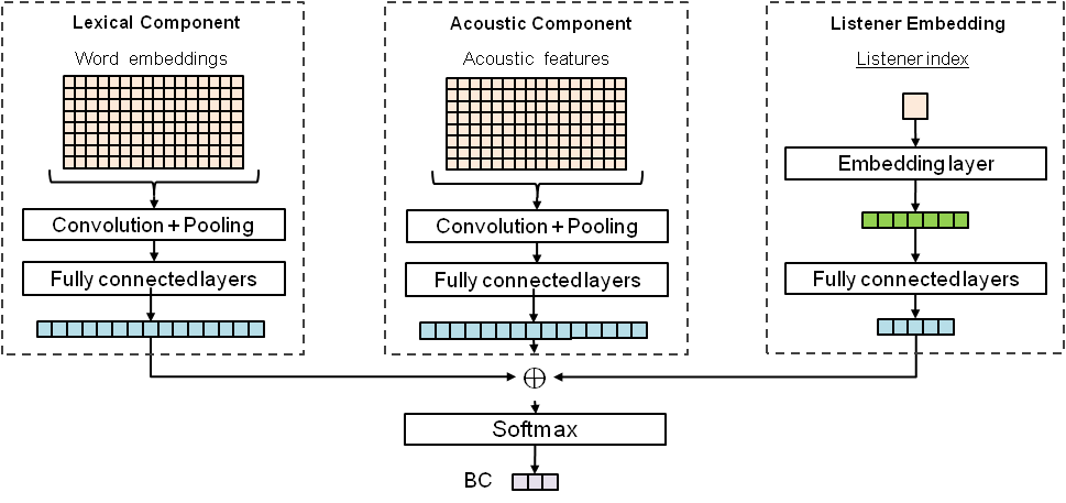
Fig. 1: Backchannel predictor’s model. $\oplus$ represents a concatenation.

The lexico-acoustic component, i.e. the bi-CNN constituent, is based on [18]. The lexical input consists of a grid-like representation made by stacking up the word embeddings of the $n$ previous speaker’s words given a certain time point in the conversation. Similarly, given that time point, acoustic features at frame level of the last 2000 ms are extracted from the frontchannel and stacked up. Each input is processed by a CNN that generates a vector representation.

CNNs perform a discrete convolution using a set of different filters on an input matrix, where each column of the matrix is the word embedding of the corresponding word. We use 2D filters $f$ (with width $|f|$) spanning over all embedding dimensions $d$ as described by the following equation:

$$(w\ast f)(x,y)=\sum_{i=1}^{d}\sum_{j=-|f|/2}^{|f|/2}w(i,j)\cdot f(x-i,y-j)$$ (1)

The third model’s input is single integer, that represents the unique identifier for the listener. That integer is passed to a embedding layer, that stores the listeners’ vector representation, followed by two FFNs. Note that lexical and acoustic information are not aligned as in other works. Our intuition is that the lexical meaning and the acoustic cues should be processed separately, so that both sources are not constrained during the training. Finally, the three resulting vectors are concatenated and passed to a softmax layer, that outputs a probability distribution over the three classes: No-BC, BC-Continuer and BC-Assessment.

3 Experimental setup

3.1 Data and setup for BC prediction

3.1.1 Backchannel data annotation

We evaluate our model on SWBD [17], a dialog corpus of telephone conversations. Annotations and time stamps for BC are taken from [19], and further expanded by following the setup proposed by Ruede et al. [15]. We also took the time stamps for No-BC instances from [15] as well as the spĺits. From a total of 2438 conversations, 2000 are for training, 200 for validation and 238 for test. As result, our data consists of almost 61k BC instances and the same amount for No-BC.

However, we decided to take the classification to be consistent with the BC categorization proposed in [10], i.e continuer vs assessment BCs. Since the The Switchboard Dialog Act Corpus (SwDA) data is not annotated in such a way, we manually annotated them with continuer vs assessment BCs labels.

The annotation process was as follows, we extracted a list of 670 unique utterances used within the corpus to backchannel. Then, according to the theory, continuers [10, 1, 6], aka general BCs, are uh-huh, um-hum and their variations. Following that, we annotated as continuers those instances, whose realization contained exclusively these words or their variations, while ignoring filter noise or other markers; the rest was annotated as assessment. As result, only 68 out of 670 unique BC realizations were annotated as continuers. However, the distribution in the dataset among both BC classes is almost balanced: No-BC 50%, BC-Continuer 22.5% and BC-Assessment 27.5%.

For listener annotation, we obtain from SWBD corpus the mapping between dialog channels and unique speakers. On average, each speaker takes part in 10 conversations. Although the official SWBD documentation reports 543 speakers, the annotation did not include speakers for 11 channels. Pragmatically, we linked those channels to a random speaker. In total, our model learns 519 listener embeddings.

3.1.2 Backchannel data extraction

As mentioned in subsubsection 3.1.1, we obtained the time stamps for all instances in the dataset, that were later used to extract both lexical and acoustic features.

Lexical information refers to 15 previous words from the frontchannel that happened before the time stamp that marks the instance in the backchannel. We used setup from [15] to extract the words from MTs. ATs were generated by our ASR system described in subsection 3.2.

Time stamps are also used to obtain acoustic features of the 2000 ms from the frontchannel speech signal before the BC happens. Acoustic features are extracted at frame level, i.e. the speech signal is divided into frames of 25 ms with a shift of 10 ms. Two types of acoustic features were extracted using the openSMILE toolkit [20]: 3 prosodic features (fundamental frequency, loudness and voicing probability), 13 Mel-frequency cepstral coefficients.

3.2 Data and setup for ASR

We employed KALDI [21] to build the hybrid TDNN/HMM ASR system [22, 23]. To the extent of our knowledge, it is one of the best hybrid ASR systems available for research and thus was selected for our experiments. In the recipe, 40 MFCCs were computed at each time step and each frame was appended to a 100-dimensional iVector. Speaker adaptive feature transform techniques and data augmentation techniques were implemented. The alignments are based on the Gaussian Mixture Model (GMM)/HMM model with linear discriminant analysis (LDA) [24], maximum likelihood linear transform (MLLT) [25] and speaker adaptive training (SAT) [26, 27]. Besides, the language mode is 3-gram trained with the transcriptions. The word error rate (WER) of this hybrid TDNN/HMM system on train, validation and test sets are 16.88%, 16.89% and 20.51%, respectively.

4 Experimental results

Hyperparameter	LM	AM
Filter widths	3, 4, 5	11, 12
Number of filters	16	16
Dropout rate	0.5	0.5
Activation function	ReLU	ReLU
Pooling size	(50, 1)	(18, 1)
Word embeddings	word2vec [28]	—
Acoustic features	—	Prosodic & MFCC
Number of frames	—	148 & 198
Mini-batch size	64	64

Table 1: Hyperparameters.

We present the results from three models, i.e. the acoustic model that takes only acoustic features, the lexical model that only takes word embeddings and the lexico-acoustic model (Figure 1) that takes both inputs and the listener embedding. Their hyperparameters are presented in Table1. The listener embedding is a 5-dimension vector.

4.1 Acoustic model

Table 2 summarizes the results obtained from training and testing only the acoustic component on prosodic and MFCC features at with different number of frames, i.e. 148 and 198 frames representing 1.5 s and 2 s, respectively. In both scenarios, MFCC features yield better results. The best performance occurs when 148 frames are fed into the acoustic model. Therefore, we experimented further only using MFCC features and 148 frames.

Time	Features
	Prosodic	MFCC
1.5 s (148 frames)	53.7	54.7
2.0 s (198 frames)	52.9	54.2

Table 2: Accuracy results (%) on acoustic model.

4.2 Lexical model

Experiments with the lexical component had the goal of finding the appropriate number of words from the frontchannel. We tested from 5-10 and the best performance was found with 5 words, in both scenarios - MTs and ATs (see Table 3). This hyperparameter was then used for further experiments.

Words	Transcriptions
	Manual	Automatic
5	53.9	53.7
6	53.6	53.1
7	52.2	53.0

Table 3: Accuracy results (%) on lexical model.

4.3 Lexico-acoustic model

Table 4 summarizes our experimental results in accuracy terms obtained from three models (acoustic, lexical and lexico-acoustic) in different configurations: no listener vs. with listener and MTs vs. ATs. Models were tested on the same type of transcriptions used for training, no cross-transcriptions was performed. However, experimental results in [18] suggest to train and test on the same type of data.

Model	No listener		With listener
	MTs	ATs	MTs	ATs
Acoustic	54.7		57.1
Lexical	53.9	53.7	56.3	55.8
Lexico-acoustic	56.7	56.4	58.9	58.6

Table 4: Global accuracy results (%).

5 Discussion & Analysis

5.1 Discussion

Overall, our results indicate that the combination of lexical and acoustic information leads to the best performance, reaching 58.9% when the model was trained on MTs and the listener embedding was present. Furthermore, listener embeddings contribute to a consistent improvement.

A surprising finding is that the acoustic model outperforms the lexical one, regardless of the use of MTs or ATs in the latter model. This contradicts the findings from dialog act tagging [18], where lexical information carries more important cues, however, both tasks are not completely comparable.

Another interesting finding is that the performance difference in the lexical model between MTs or ATs is relatively small, although the WER in the ASR system ranges from 16.9% to 20.5%. A deeper analysis is still needed to find out which lexical information is valuable in the ASR transcriptions.

5.2 Analysis

In order to understand deeper our results and their implications, we present a confusion matrix (Figure 2) of the lexico-acoustic with listener embedding on ATs.

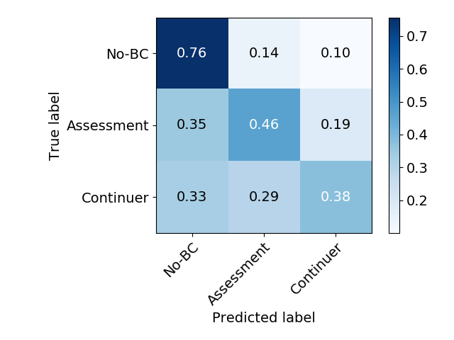
Fig. 2: Confusion matrix for the best results on ATs

Our model failed at predicting No-BC almost the half of the time, instead of the two other classes. We can assume that the model, seen as a listener, was acting tentative to backchannel, so that one of the future work could be to introduce a parameter in the model to control the backchanneling rate.

Focusing on BC classes, the model was able to distinguish between assessment and continuer. However, our system failed more at predicting continuers. A deeper research at lexical and prosodic levels should be carried out, in order to understand the contextual differences that trigger each of them.

6 Conclusion

We investigated modeling backchanneling from listener perspectives in conversations motivated by proactive backchanneling theory, which suggests different categories of backchanneling and how they influence speakers. We proposed a model that combines lexical and acoustic cues and introduces a simple but novel method of using listener embeddings to mimic different backchanneling behaviours. Our experimental results on the Switchboard benchmark data set show several interesting findings: 1) acoustic cues are more important than lexical cues in this task, 2) listener embeddings are useful to improve the overall performance and 3) our proposed model is robust against ASR errors.

References

- [1] A. Bangerter and H. Clark, “Navigating joint projects with dialogue,” Journal of Cognitive Science, 2003.
- [2] Victor Yngve, “On getting a word in edgewise,” in Proc. of CLS 16, 1970.
- [3] Lawrence J Brunner, “Smiles can be back channels,” Journal of Personality and Social Psychology, 1979.
- [4] J. B. Bavelas and J. Gerwing, “The listener as addressee in face-to-face dialogue,” Journal of Listening, 2011.
- [5] R. Bertrand, G. Ferré, P. Blache, R. Espesser, and S. Rauzy, “Backchannels revisited from a multimodal perspective,” in Proc. of AVSP, 2007.
- [6] J. Tolins and J. E F. Tree, “Addressee backchannels steer narrative development,” Journal of Pragmatics, 2014.
- [7] P. M Clancy, S. A Thompson, R. Suzuki, and H. Tao, “The conversational use of reactive tokens in english, japanese, and mandarin,” Journal of Pragmatics, 1996.
- [8] H. H Clark and M. A Krych, “Speaking while monitoring addressees for understanding,” Journal of Memory and Language, 2004.
- [9] Emanuel A. Schegloff, “Discourse as an interactional achievement: some uses of ’uh huh’ and other things that come between sentences,” in Analyzing Discourse: Text and Talk, p. 71–93. Georgetown University Press, 1982.
- [10] Charles Goodwin, “Between and within: Alternative sequential treatments of continuers and assessments,” Journal of Human Studies, 1986.
- [11] Nigel Ward, “Using prosodic clues to decide when to produce back-channel utterances,” in Proc. of ICSLP, 1996, pp. 1728–1731.
- [12] N. Ward and W. Tsukahara, “Prosodic features which cue back-channel responses in english and japanese,” Journal of Pragmatics, pp. 1177–1207, 2000.
- [13] L.-P. Morency, I. de Kok, and J. Gratch, “A probabilistic multimodal approach for predicting listener backchannels,” Journal of Autonomous Agents and Multi-Agent Systems, pp. 70–84, 2010.
- [14] L. Huang, L.-P. Morency, and J. Gratch, “Learning backchannel prediction model from parasocial consensus sampling: a subjective evaluation,” in Proc. of ACM IVA, 2010.
- [15] R. Ruede, M. Müller, S. Stüker, and A. Waibel, “Enhancing backchannel prediction using word embeddings.,” in Proc. of Interspeech, 2017.
- [16] Bettina Heinz, “Backchannel responses as strategic responses in bilingual speakers’ conversations,” Journal of Pragmatics, 2003.
- [17] John J Godfrey et al., “Switchboard: Telephone speech corpus for research and development,” in Proc. of ICASSP, 1992.
- [18] D. Ortega and N. T. Vu, “Lexico-acoustic neural-based models for dialog act classification,” in Proc. of ICASSP, 2018.
- [19] D. Jurafsky and E. Shriberg, “Switchboard swbd-damsl shallow-discourse-function annotation coders manual,” Institute of Cognitive Science Technical Report, 1997.
- [20] F. Eyben, F. Weninger, F. Gross, and B. Schuller, “Recent developments in opensmile, the munich open-source multimedia feature extractor,” in Proc. of ACM Multimedia, 2013.
- [21] Daniel Povey et al., “The Kaldi speech recognition toolkit,” in Proc. of IEEE ASRU, 2011.
- [22] A. Waibel, T. Hanazawa, G. Hinton, K. Shikano, and K. J Lang, “Phoneme recognition using time-delay neural networks,” Proc. of ICASSP, 1989.
- [23] Daniel Povey et al., “Purely sequence-trained neural networks for ASR based on lattice-free MMI,” in Proc. of Interspeech, 2016.
- [24] R. O. Duda, P. E. Hart, and D. G. Stork, Pattern classification, Wiley, 2000.
- [25] R.A. Gopinath, “Maximum likelihood modeling with gaussian distributions for classification,” in Proc. of IEEE ICASSP, 1998.
- [26] M. J. F. Gales, “Maximum likelihood linear transformations for hmm-based speech recognition,” Journal of Comp.Speech & Language, 1998.
- [27] S. Matsoukas, R. Schwartz, H. Jin, and L. Nguyen, “Practical implementations of speaker-adaptive training,” in Proc. of DARPA Speech Recognition Workshop, 1997.
- [28] T. Mikolov, I. Sutskever, K. Chen, G. Corrado, and J. Dean, “Distributed representations of words and phrases and their compositionality,” arXiv preprint arXiv:1310.4546, 2013.
- AdaGrad
- adaptive gradient algorithm
- AM
- attention mechanism
- CRF
- conditional random field
- CNN
- convolutional neural network
- FFN
- feed-forward network
- DA
- dialog act
- DL
- deep learning
- E2E
- End-to-End
- SGD
- stochastic gradient descent
- HMM
- hidden Markov model
- NLP
- natural language processing
- RNN
- recurrent neural network
- SVM
- support vector machine
- SWBD
- Switchboard Corpus
- SwDA
- The Switchboard Dialog Act Corpus
- ASR
- automatic speech recognition
- NN
- neural network
- MTs
- manual transcriptions
- ATs
- automatic transcriptions
- E2E
- End-to-End
- CD
- context-dependent
- TDNN
- time-delay neural network
- CTC
- connectionist temporal classification
- WER
- word error rate
- MFCC
- Mel-frequency cepstral coefficient
- GMM
- Gaussian Mixture Model
- ESPnet
- End-to-End Speech Processing Toolkit
- BC
- backchannel