The GAPS programme at TNG

Abstract

Context. Massive substellar companions orbiting active low-mass stars are rare. They, however, offer an excellent opportunity to study the main mechanisms involved in the formation and evolution of substellar objects.

Aims. We aim to unravel the physical nature of the transit signal observed by the TESS space mission on the active M dwarf TOI-5375.

Methods. We analysed the available TESS photometric data as well as high-resolution (R $\sim$ 115000) HARPS-N spectra. We combined these data to characterise the star TOI-5375 and to disentangle signals related to stellar activity from the companion transit signal in the light-curve data. We ran an MCMC analysis to derive the orbital solution and apply state-of-the-art Gaussian process regression to deal with the stellar activity signal.

Results. We reveal the presence of a companion in the brown dwarf / very-low-mass star boundary orbiting around the star TOI-5375. The best-fit model corresponds to a companion with an orbital period of 1.721564 $\pm$ 10^-6 d, a mass of 77 $\pm$ 8 $M_{\rm J}$ and a radius of 0.99 $\pm$ 0.16 $R_{\rm J}$.

Conclusions. We derive a rotation period for the host star of 1.9692 $\pm$ 0.0004 d, and we conclude that the star is very close to synchronising its rotation with the orbital period of the companion.

1 Introduction

Almost thirty years after the discovery of the first exoplanets (Wolszczan & Frail, 1992; Mayor & Queloz, 1995), thousands of planetary systems have been discovered showing an astonishing diversity of orbits, compositions, and host stellar properties. Understanding the origin of this diversity is one of the major goals of modern Astrophysics. Young stars are valuable targets that offer the unique opportunity to provide observational constraints on the timescales involved in the formation and migration of planets in close orbits, the physical evolution of the planets, as well as atmospheric evaporation due to the strong X and UV irradiation of the host star. Planets have been found in young stellar clusters (e.g. Malavolta et al., 2016; Rizzuto et al., 2017), young stellar kinematic groups (e.g. Benatti et al., 2019; Newton et al., 2019; Nardiello et al., 2022) as well as single young stars (e.g. Plavchan et al., 2020; Carleo et al., 2021). However, the detection and characterisation of planets around young stars via radial velocity or transit methods are challenging due to the high-activity levels of the host stars and some previously claimed planets have been retracted after detailed analysis (e.g. Carleo et al., 2018; Damasso et al., 2020). Furthermore, high rotation rates or variability due to pulsations might also challenge the detection of planets around young stars. As a consequence, the sample of known, well-characterised young exoplanets is still rather limited.

On the other hand, M dwarfs have been recognised as promising targets to search for small, rocky planets with the potential capabilities of host life (e.g. Dressing & Charbonneau, 2013, 2015). While small planets orbiting around M dwarfs seem to be abundant (e.g Howard et al., 2012; Bonfils et al., 2013; Tuomi et al., 2014), results from radial velocity surveys show that, unlike their FGK counterparts, the frequency of gas-giant planets orbiting around low-mass stars is low (Endl et al., 2006; Butler et al., 2006; Cumming et al., 2008; Pinamonti et al., 2022). This result might be understood in the framework of core-accretion models for planet formation. Within this scenario, the low-mass protoplanetary disc of an M dwarf conspires against the formation of gas-giant planets. However, using data from the Transiting Exoplanet Survey Satellite (TESS, Ricker et al., 2015), a small number of transiting gas-giant planets orbiting around low-mass stars has been discovered. Some examples include TOI-1728 b (Kanodia et al., 2020), TOI-442 b (Dreizler et al., 2020) and TOI-3757 b (Kanodia et al., 2022), among others. All these planets have close-in orbits and constitute valuable targets to help us in our understanding of planet formation and migration. While it was proposed early on that close-in gas-giant planets should form beyond the snowline and then experience subsequent inward migration (e.g. Lin et al., 1996), the in-situ formation of gas-giant planets has been recently revisited (Batygin et al., 2016; Boley et al., 2016; Maldonado et al., 2018). In addition to planetary companions, M dwarfs can also host brown dwarfs in close orbits. Recent works have discussed differences in the period-eccentricity distribution of massive ($M_{\rm P}$ $>$ 45 $M_{\rm J}$) and low-mass brown dwarf ($M_{\rm P}$ $<$ 45 $M_{\rm J}$) companions, as well as in the chemical composition of their respective host stars (Ma & Ge, 2014; Mata Sánchez et al., 2014; Maldonado & Villaver, 2017). It has been shown that massive brown dwarfs have longer periods and larger eccentricities and their host stars do not show the so-called metal-rich signature. According to this scenario, massive brown dwarfs should be mainly formed in the same way as low-mass stars (by the fragmentation of a molecular cloud). On the other hand, low-mass brown dwarfs might be formed at high-metallicities by core-accretion or by gravitational instability in low-metal environments (Maldonado & Villaver, 2017). Furthermore, since these companions are massive and close to their host stars, tidal interactions between the companion and the host star are expected to constrain the evolution of the system (e.g. Mathieu & Mazeh, 1988; Mazeh, 2008; Barker, 2020; Alvarado-Montes, 2022).

In this paper, we report the validation and the confirmation of a transiting low-mass companion ($M_{\rm p}$ $\sim$ 77 $M_{\rm J}$) around the very active M0.5 dwarf TOI-5375 by using space-based photometric observations from TESS combined with high-precision radial velocities from the ground. Given the high activity levels of TOI-5375, this star has a good chance to be young. TESS identified a candidate with a radius of 1.04 $\pm$ 0.03 $R_{\rm J}$. A companion with such a radius, if confirmed, could be a giant planet, a brown dwarf or even a very low-mass star. As discussed, a giant planet transiting an active M dwarf is of special interest. Therefore, we included TOI-5375 in the sample of the GAPS-Young program (Carleo et al., 2020) in order to perform the validation and the mass determination of the transiting candidate. Our radial velocity (RV) monitoring shows that the companion is actually a massive brown dwarf or a very low mass star. The system represents a remarkable case study as it is observed in the evolutionary phase in which the star is close to synchronising its rotation with the orbital period of the companion.

This paper is organised as follows. The photometric and spectroscopic data analysed in this paper are presented in Sect. 2. We note that the star is very faint for high spectral resolution observations with 4m-class telescope, resulting in low signal-to-noise ratio (S/N) spectra. Therefore, the extraction of RVs in this regime is discussed in this section by comparing different methods. Section  3 reviews the stellar properties of TOI-5375. Sect. 4 describes the modelling of the photometric and radial velocity variations. The results are discussed at length in Sect. 5. Our conclusions follow in Sect. 6.

2 Observations

2.1 TESS photometry

TOI-5375 was observed photometrically by TESS in short-cadence mode (120 seconds) in sectors 40, 47, 53, and 60. In this work, we use the light curves extracted from all these datasets. We use the data corrected for time-correlated instrumental signatures, that is, the PDCSAP flux. The corresponding light curve is shown in figure 1. We note that the star was also observed in sectors 20 and 26. However, only HLSP data is available from these sectors. Therefore, unless otherwise noticed, data from sectors 20 and 26 are not included in the analysis.

The light curve shows a clear modulation that we attribute to the rotation of the star. A search for periodicities by using the generalised Lomb-Scargle periodogram (GLS, Zechmeister & Kürster (2009)) reveals a clear peak at 1.9692 $\pm$ 0.0004 d that corresponds to the rotation period of the star, as shown in Fig. 2. Superimposed on the rotational modulation, the light curve shows periodic transit-like signals, due to a possible substellar companion.

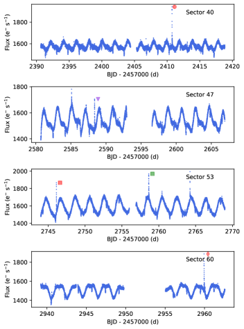
Figure 1: Original TESS photometry time series. The energetic events discussed in Sect. 4.6 are shown with different symbols according to their Sector. Within each Sector, different colours indicate that the event occurs at a different period (when phase-folded to the stellar rotation period).

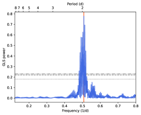
Figure 2: GLS periodogram of the TESS photometry dataset. Values corresponding to a False Alarm Probability (FAP) of 10, 1, and 0.1% are shown with horizontal grey lines. The vertical line indicates the period at 1.9692 d.

2.2 Ground-Based Photometry

Two transits of TOI-5375 were observed on October 25th and December 19th, 2022 by the TASTE program, a long-term campaign to monitor transiting planets (Nascimbeni et al., 2011). The AFOSC camera, mounted on the Copernico 1.82-m telescope at the Asiago Astrophysical Observatory in northern Italy, was purposely defocused up to $8"$ FWHM to avoid saturation and increase the photometric accuracy. Frames were acquired through a Sloan $r^{\prime}$ filter and with a constant exposure time of 15 s. A pre-selected set of suitable reference stars was always imaged in the same field of view to perform differential photometry. Unfortunately, during the first transit, the sky transparency was highly variable through the series and thick clouds passed by during the second half of the transit (egress included).

We reduced the Asiago data with the STARSKY code (Nascimbeni et al., 2013), a software pipeline specifically designed to perform differential photometry on defocused images. After a standard correction through bias and flat-field frames, the size of the circular apertures and the weights assigned to each reference star are automatically chosen by the code to minimise the photometric scatter of our target. The time stamps were uniformly converted to the BJD-TDB standard following the prescription by Eastman et al. (2010). The final (unbinned) light curves are shown in Fig. 13.

2.3 Radial velocity observations

A total of 9 HARPS-N (Cosentino et al., 2012) observations of TOI-5375 were collected in the period between BJD = 2459704 d and BJD = 2459718 d (May 4 - 18, 2022). HARPS-N spectra cover the wavelength range 383–693 nm with a resolving power of R $\sim$ 115 000. The observations were performed within the framework of the Global Architecture of Planetary Systems (GAPS) project (Covino et al., 2013). Data were reduced using the HARPS-N Data Reduction Software (DRS, Lovis & Pepe, 2007; Dumusque et al., 2021) that takes into account the usual procedures involved in échelle spectra reduction (bias level, flat-fielding, order extraction and wavelength calibration, as well as merging of individual orders). Radial velocities are computed by cross-correlating the spectra of the target star with an optimised binary mask (Baranne et al., 1996; Pepe et al., 2002). However, this procedure might not be optimal for a star like TOI-5375. To start with, TOI-5375 is an M dwarf-type star and the spectra of M dwarfs suffer from heavy blends. Side-lobes appear in the CCF that might affect the RV precision (e.g. Rainer et al., 2020). In addition, TOI-5375 is a very faint star (V $\sim$ 14 mag). This might have an effect on the selection of an appropriate mask to perform the CCF. In the M2 mask, all lines have roughly a similar weight, so weak (not deep enough) lines are lost in the not-well-defined continuum that characterises the spectra of an M dwarf, adding noise to the CCF profile. In contrast, if the K5 mask is used, only deep lines are considered and the CCF profile becomes less noisy. Furthermore, high levels of stellar activity might deform the core of the average line profile, while stellar rotation broadens the lines. Therefore, special care should be taken in selecting the half-window of the CCF in order to include the continuum when fitting the CCF profile (see e.g. Damasso et al., 2020). In addition, since we are dealing with a very red object, the signal in the bluest part of the spectra is very low, so the analysis should be limited to the red part of the spectrum. In order to illustrate these effects, we compare the RVs obtained with the DRS by using the K5 and M2 masks as well as the K5 mask with a half-window of 60 km s^-1 (instead of the default value of 20 km s^-1). The results from this comparison are given in Table 1, while in Fig. 3 we show the corresponding CCF profiles for one of our observations (we choose the one with the highest S/N, $\sim$ 13 at spectral order 46, 548 - 554 nm). It is clear from the figure that the CCF profile obtained with the M2 mask is comprised only by noise, without any visible signal. The CCF profile obtained with the original K5 mask, although asymmetric has a Gaussian-sharp form but lacks a good continuum for a proper fitting. The enlarged-window K5 mask, on the other hand, provides a better fit to a Gaussian function with a lower error. These calculations have been done by using the DRS version implemented through the YABI interface (Hunter et al., 2012) at the Italian Centre for Astronomical Archives.

Table 1: Comparison between the different methods used to extract the RVs.

Method	Mask	$\overline{RV}$	$\overline{\Delta{RV}}$	rms
		(km s-1)	(km s-1)	(km s-1)
CCF	M2	-65.05	0.12	9.94
CCF	K5	-59.53	0.09	17.18
CCF	K5 w60	-61.35	0.06	12.85
TERRA			0.04	0.506
SERVAL			0.16	0.99
LSD		-59.63	0.36	12.42
SpotCCF		-59.57	0.32	12.30

RVs were also computed with the Java-based Template-Enhanced Radial velocity Re-analysis Application (TERRA Anglada-Escudé & Butler, 2012). TERRA measures the RVs by a least-square match of the observed spectrum to co-added high S/N template spectra derived from the same observations. The bluest part of the spectra was excluded from the analysis and only orders with $\lambda$ $>$ 434 nm were considered. It has been shown that for M dwarf stars the RVs derived by TERRA show a lower root-mean-square (rms) than the DRS and should be preferred (Perger et al., 2017). However, we note that in the case of TOI-5375 the rms of the RVs obtained by using TERRA is $\sim$ 34 times lower than the rms obtained when using the RVs derived by the DRS. While the CCF RVs show a rms between 9.9 and 17 km s^-1 (depending on the mask considered), TERRA RVs show a rms of only 0.5 km s^-1. TERRA RVs are not consistent with the RVs variations seen in the spectra. A quick look shows that spectral lines show relative shifts between different nights of the order of several km s^-1. A possible explanation for this discrepancy might be related to the low S/N of our spectra. It is likely that TERRA identifies some of the noise as “true” spectral features. In order to check this fact, we made use of the SpEctrum Radial Velocity AnaLyser tool (SERVAL, Zechmeister et al., 2018). The concept behind SERVAL is similar to TERRA, but it constitutes an alternative implementation. Again, we derive RVs that show a very low rms ($\sim$ 1 km s^-1). Therefore, we decided to exclude the TERRA and SERVAL RVs from our analysis.

In order to avoid the aforementioned difficulties we decided to derive RVs using a self-written python package which computes the mean line profile using the least-squares deconvolution technique (LSD, Donati et al., 1997) with a stellar mask obtained from the VALD3 database (Piskunov et al., 1995; Ryabchikova et al., 2015) with appropriate stellar parameters for TOI-5375. The mean line profiles are then fitted with a rotational broadening function. Further details can be found in Rainer et al. (2021). An example of one of the derived LSD profiles is shown in Figure 3 where it can be compared with the CCF profiles obtained by the DRS. The LSD derived RVs have a rms of 12.42 km s^-1 and a mean uncertainty of 0.36 km s^-1. Figure 4 shows a comparison between the RVs velocities obtained by using different masks and methods. We note that the RVs derived with the enlarged-window K5 mask are similar to the ones derived with the LSD technique. This shows that by performing an appropriate mask and half-window selection it is possible to derived precise RVs using the CCF method even in spectra at low S/N or for the case of fast rotators. As mentioned, RVs based on the template-matching algorithm (TERRA and SERVAL) provide rather flat RV curves when compared with the CCF and LSD values. We note that the CCF and LSD techniques combine the spectral lines to create a mean profile, thus it should be possible to achieve a reasonable S/N. In fact, the S/N of the CCF increases roughly as $\sqrt{N}$ where $N$ is the number of stellar lines used to compute the CCF (typically of the order of several thousands of lines). On the other hand, it seems that the template-matching algorithm, when all the observed spectra have a low S/N, is not able to generate a suitable template to compute accurate RVs. Finally, RVs were also computed from the LSD profiles by using the SpotCCF software (Di Maio et al. in prep.) which takes into account the presence of multiple spots on the stellar surface. It also accounts for the wings of the LSD profile by convolving the rotational profile with a Lorentzian profile. The code was run without considering any spot. We find that the SpotCCF-derived RVs are quite similar to the ones derived from the LSD analysis, thus confirming the reliability of our measurements. The analysis presented in the following refers to the LSD-derived RVs.

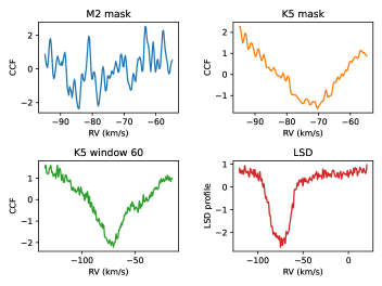
Figure 3: Examples of standardised (mean subtracted and division by the standard deviation) CCF profiles obtained by the DRS using different binary masks as well as the LSD profile.

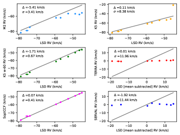
Figure 4: RVs obtained using different masks and methods versus LSD RVs. For TERRA and SERVAL RVs, we subtracted the mean LSD RV for the comparison. Each panel shows the mean value and standard deviation of the difference RVs other methods - LSD RVs. Gray lines show the one-to-one relationship.

3 The host star

TOI-5375 (a.k.a. TIC 71268730, 2MASS J07350822+7124020, 1RXS J073508.9+712415) is a M0.5 dwarf located at a distance of 121.65 $\pm$ 0.17 pc from the Sun (Gaia Collaboration, 2022). Its main stellar properties are listed in Table 2. Stellar effective temperature, spectral-type and metallicity are determined from a methodology based on the use of a principal component analysis and sparse Bayesian fitting methods, which make use of the same spectra used in this work for the radial velocity analysis (see Sec. 2). In brief, a relationship between the principal components and the stellar parameters is derived by training the data with the spectra of M dwarfs orbiting around an FGK primary or M dwarfs with effective temperature obtained from interferometric measurements of their radii. Further details can be found in Maldonado et al. (2020). We also compute T_eff and [Fe/H] by using photometric relationships (Casagrande et al., 2006; Neves et al., 2012). We note that the photometric T_eff is significantly lower than the spectroscopic one. This discrepancy has already been noted and discussed (see e.g. Maldonado et al., 2015, and references therein). It is related to the fact that M dwarfs emission deviates from a blackbody for wavelengths beyond $\sim$ 2 $\mu$m. The photometric estimate of [Fe/H] is also lower than the spectroscopic one. In a recent work, Maldonado et al. (2020) show that the use of photometric estimates for M dwarfs gives a [Fe/H] distribution that is shifted towards lower values when compared with an otherwise similar sample of FGK stars. Therefore, spectroscopic parameters are preferred, although we caution against the relatively low S/N of our spectra (of the order of 44 in the 604-605 nm region, measured in the coadded spectra). Stellar mass is computed following the relations based on near-infrared photometry by Henry & McCarthy (1993), while the stellar radius is obtained using the mass-radius relationship provided by Maldonado et al. (2015). From the stellar mass and radius values, the surface gravity was estimated. The stellar luminosity is computed by using the bolometric corrections provided by Flower (1996).

Table 2: Physical properties of TOI-5375.

Parameter	Value	Notes
$\alpha$ (ICRS J2000)	07:35:08.22	a
$\delta$ (ICRS J2000)	+71:24:02.13	a
Spectral Type	M0.5	b
Teff spec (K)	3885 $\pm$ 25	b
Teff phot (K)	3709 $\pm$ 27	b
${\rm[Fe/H]}$ spec (dex)	+0.26 $\pm$ 0.04	b
${\rm[Fe/H]}$ phot (dex)	+0.03 $\pm$ 0.03	b
$M_{\star}$ ($M_{\odot}$)	0.64 $\pm$ 0.10	b
$R_{\star}$ ($R_{\odot}$)	0.62 $\pm$ 0.10	b
$\log g$ (cm s-2)	4.66 $\pm$ 0.15	b
$\log(L_{\star}/L_{\odot})$	-1.19 $\pm$ 0.15	b
Prot (d)	1.969226 $\pm$ 0.000358	b
veq (km s-1)	15.9 $\pm$ 2.6	b
$\pi$ (mas)	8.2202 $\pm$ 0.0114	a
$\mu_{\alpha}$ (mas/yr)	48.434 $\pm$ 0.009	a
$\mu_{\delta}$ (mas/yr)	19.069 $\pm$ 0.012	a
vrad (km s-1)	-61.59 $\pm$ 0.16	b
$U$ (km s-1)	61.15 $\pm$ 0.11	b
$V$ (km s-1)	-30.37 $\pm$ 0.08	b
$W$ (km s-1)	-5.68 $\pm$ 0.08	b
$B$ (mag)	15.418 $\pm$ 0.106	c
$V$ (mag)	14.063 $\pm$ 0.056	c
2MASS J (mag)	11.167 $\pm$ 0.022	d
2MASS H (mag)	10.480 $\pm$ 0.023	d
2MASS KS (mag)	10.302 $\pm$ 0.020	d
GAIA DR3 G (mag)	13.410046 $\pm$ 0.003056	a
GAIA DR3 BP (mag)	14.336692 $\pm$ 0.006075	a
GAIA DR3 RP (mag)	12.448772 $\pm$ 0.005159	a
WISE1 (mag)	10.226 $\pm$ 0.023	e
WISE2 (mag)	10.212 $\pm$ 0.021	e
WISE3 (mag)	10.354 $\pm$ 0.084	e
WISE4 (mag)	$>$ 8.543	e

The rotational period is computed from the analysis of the TESS light curve (see Sec. 2) while the equatorial velocity is estimated from the rotation period and the stellar radius. The available photometry for TOI-5375 has been used to build and trace the star spectral energy distribution along with PHOENIX/BT-SETTL atmospheric models (Allard et al., 2012), see Fig. 5.

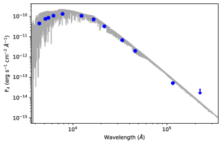
Figure 5: Spectral energy distribution of TOI-5375. A PHOENIX/BT-SETTL atmospheric model (T_eff = 3885 K, $\log g$ = 4.66 cm s^-2, [Fe/H] = +0.26 dex) is overplotted. Errors in the observed fluxes are within the symbol’s size.

3.1 Age estimates

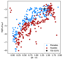
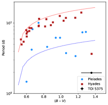
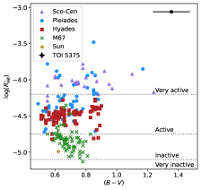
Figure 6: Age diagnostics for TOI-5375. Left: Fractional X-ray luminosity $\log(L_{\rm X}/L_{\rm Bol})$ vs. colour index (B - V). Centre: Rotation period as a function of the (B - V) colour. Two gyrochrones (at the ages of the Pleiades and the Hyades) have been overplotted for comparison. Right: $\log$(R’_HK) vs. colour index (B - V). Dashed lines are the limits for very active, active, inactive, and very inactive stars, according to Henry et al. (1996).

Stellar age is one of the most difficult parameters to determine in an accurate way, even for main-sequence solar-type stars, as they evolve too slowly to be dated by their position in the Hertzsprung-Russell Diagram. For solar-type stars, it is well known that stellar activity and rotation are related by the stellar dynamo (e.g. Noyes et al., 1984) and both activity and rotation diminish as the star evolves and loses angular momentum. Thus, activity and rotation tracers, such as Ca emission, X-ray, or rotation periods, are often used to estimate stellar ages (see e.g. Mamajek & Hillenbrand, 2008). However, in this case, the rotation of TOI-5375 is being accelerated by the tides raised by the companion (as we will discuss in Sect. 5). As a consequence, the star can show a high level of chromospheric or X-ray emission despite being rather old. Therefore, age diagnostics based on the rotation period will only provide lower limits to the age of the TOI-5375 system. In the following, we consider as “young” those stars with an age younger than the Hyades, $\sim$ 750 Myr.

To compute the $L_{\rm X}$ of TOI-5375 we search for an X-ray counterpart in the ROSAT All-Sky Bright Source Catalogue (Voges et al., 1999) and apply the count rate-to-energy flux conversion factor relation given by Fleming et al. (1995). The derived X-ray luminosity is $\log L_{\rm X}$ = 29.44 $\pm$ 0.22 erg s^-1, while the position of TOI-5375 in the $\log(L_{\rm X}/L_{\rm Bol})$ versus colour index (B - V) plane is shown in Fig. 6 (left). Bolometric corrections are derived from the (B-V) colour by interpolating in Flower (1996, Table 3). Data from the Pleiades, age $\sim$ 112 Myr (Stauffer et al., 1994) and Hyades, age $\sim$ 750 Myr (Stern et al., 1995) are overplotted for comparison. The position of TOI-5375 in this diagram is consistent with the position of the Pleiades.

Figure 6 (centre) shows the rotation period of TOI-5375 as a function of the colour index (B-V). For comparison, data from the Pleiades (Prosser et al., 1995) and from the Hyades (Radick et al., 1987) are overplotted. Two gyrochrones (at the ages of the Pleiades and the Hyades) are also overplotted. The figure seems to indicate that TOI-5375 is a young star with a fast rotation period.

TOI-5375 shows a clear emission in the Ca ii H & K lines. Balmer lines (from H$\alpha$ to H$\epsilon$), as well as other known activity indexes such as the Na i D₁, D₂ doublet and the He i D₃ line are also shown in emission. To quantify the stellar chromospheric activity we make use of the $\log$(R’_HK), defined as the ratio of the chromospheric emission in the cores of the broad Ca ii H & K absorption lines to the total bolometric emission (e.g. Noyes et al., 1984). We start by computing the so-called $Sindex$ which is measured in the Mount Wilson scale by the HARPS-N DRS implemented through the YABI interface. The $Sindex$ contains both the contribution of the photosphere and the chromosphere. In order to account for the photospheric correction we used the calibration based on the colour index (B-V) developed by Suárez Mascareño et al. (2015) who updated and extended the original calibration from Noyes et al. (1984) to the low-mass regime up to a (B-V) value of 1.90. The derived $\log$(R’_HK) for TOI-5375 is -3.06 $\pm$ 0.10. This value can be compared with the activity level of stars in clusters with well-known ages. The comparison is shown in Fig. 6 (right). Data from the Sco-Cen complex (age $\sim$ 5 Myr), Pleiades, Hyades, and M67 (age $\sim$ 4000 Myr) are from Mamajek & Hillenbrand (2008). TOI-5375 is located in the range of very active stars with a mean $\log$(R’_HK) higher than other stars in young stellar associations and clusters.

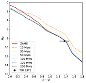
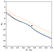
Figure 7: Colour-magnitude diagram. Left: M_V as a function of (B-V) colour. Right: M_V as a function of (V - K_S) colour.

As an additional age diagnostic we plot the position of TOI-5375 in a colour-magnitude diagram, see Fig. 7. The ZAMS position as well as several pre-main sequence isochrones (computed at metallicity +0.20 dex) from Siess et al. (2000) are plotted. We use the M_V versus (B-V) (left panel) and M_V versus (V - K_S) plots (right panel), as it has been shown that young rotating stars in the Pleiades tend to show blue excesses, that is bluer (B-V) colours, than other relatively old stars (Stauffer et al., 2003). Indeed, we note that the position of the star in the diagram, when considering the (B-V) colour, suggests an age between 30 and 200 Myr (we note the large uncertainty in B magnitude), whilst when considering the (V - K_S) colour, the position of TOI-5375 is more consistent with a younger, $\sim$ 30 Myr age.

Membership in stellar associations and young moving groups has been used as a methodology to identify young stars and to assign ages, especially after the release of the Hipparcos data (see e.g. Maldonado et al., 2010, and references therein). The Galactic spatial-velocity components $(U,V,W)$ of TOI-5375 are computed from the stellar radial velocity from our own orbital solution, together with Gaia parallaxes and proper motions (Gaia Collaboration, 2022). We follow the procedure described in Montes et al. (2001) and Maldonado et al. (2010), where the original algorithm (Johnson & Soderblom, 1987) is adapted to epoch J2000 in the International Celestial Reference System (ICRS) following Sect. 1.5 of the Hipparcos and Tycho catalogues (ESA, 1997). We made use of the full covariance matrix to compute the uncertainties. In this way, we account for the possible correlation between the astrometric parameters. The corresponding $(U,V,W)$ values are provided in Table 2, while the position of TOI-5375 in the $(U,V)$ plane is shown in Fig. 8. From the analysis of its velocity components we see that TOI-5375 is located outside the region of the young stars so we conclude that it is a field thin disc star. This conclusion is supported by the use of Bayesian methods (BANYAN, Gagné et al., 2018) that confirm that TOI-5375 is, with high-probability (99.9%), a field star. The high-metallicity content of the star might be an additional indication that the star is not young. This is because typically, the metallicity of young stars in the solar neighbourhood is close-to-solar or slightly sub-solar (Spina et al., 2017).

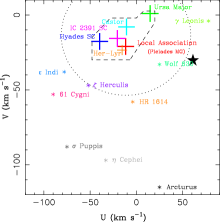
Figure 8: $(U,V)$ plane showing the position of the young disc population (dashed line) as defined by Eggen (1984, 1989) as well as the known kinematic groups (large crosses and asterisks) in the solar neighbourhood (see Maldonado et al., 2010; Maldonado, 2012, and references therein). The dotted line represents the velocity ellipsoid determined by Francis & Anderson (2009). The position of TOI-5375 is shown with a black star (uncertainties are within the symbol size). All velocities are in the Solar System reference frame.

To summarise, age estimates based on the rotation of the star seem to indicate that TOI-5375 is a young star. However, other age estimates based on the stellar metal content or the kinematics do not support this statement. The disagreement is due to the fact the stellar rotation period is being accelerated by the companion, as we shall discuss in Sect. 5. Therefore, the only conclusion that we can draw from this analysis is that TOI-5375 is a field star that should have an age older than the one of stars in young stellar associations like the Pleiades or the Hyades.

4 Analysis

4.1 Validation and vetting tests

As mentioned, the TESS photometric light curve of TOI-5375 shows clear periodic dips compatible with the transits of a substellar companion orbiting around this active, M dwarf. Because of the low spatial resolution of the TESS cameras ($\thickapprox$ 21 arcsec/pixel) some of the objects initially identified as a substellar companion might indeed be a false positive (FP). We, therefore, perform an analysis to identify possible nearby contaminating stars that might be the origin of blended eclipsing binaries (BEB). The analysis is based on the use of the photometric data provided by Gaia and is described at length in Mantovan et al. (2022).

The analysis shows that, besides TOI-5375, there is a star at 33.5 arcsec (Gaia DR2 1110586939683894528) separation from TOI-5375 that might reproduce the transit signal, see Fig. 9. To be sure that the transits are not due to contamination by this neighbour, we perform the analysis of in- or out-of-transit centroid check following the procedure described in Nardiello et al. (2020) and Nardiello (2020). Data from sectors 20 and 26 are included in this analysis. It should be noticed that the in- or out-of-transit centroid analysis is performed on the full frame images and therefore it is independent from the analysis of the light curve. The results are shown in figure 10. It can be seen that, within the errors, the in- or -out-of-transit mean centroids are in agreement with the position of TOI-5375.

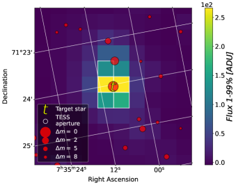
Figure 9: Gaia stars identified in the TESS field. The position of TOI-5375 is shown with the letter “t”.

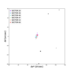
Figure 10: In- or out-of-transit centroid tests calculated for each sector. Black dots are background stars.

Finally, in order to rule out the possibility that the transiting candidate is an FP we use the VESPA software (Morton, 2012, 2015). We obtain a 100% probability of having a Keplerian transiting companion around TOI-5375, while the probability of a FP is of the order of $\sim$ 7 $\times$ 10^-10. All these analyses confirm that TOI-5375 b is fully and statistically vetted and only requires reconnaissance spectroscopy to be promoted to a “statistically validated” companion.

4.2 Photometric time series analysis

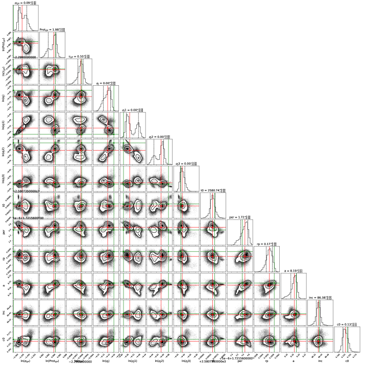
Figure 11: Posterior distributions of the Bayesian fit of the photometric time series.

In order to characterise the properties of TOI-5375 b, the photometric data were modelled by using a Bayesian framework based on a Monte Carlo sampling of the parameter space. The photometric light curve contains the contribution of the proposed planetary signal as well as the effect of the stellar activity of the host star. The stellar signal is modelled with a Gaussian process (GP) analysis. The covariance (or kernel) function adopted is a simple harmonic oscillator (SHO) kernel which is defined as follows

$$k(i,j)=\sigma_{GP}\exp\left(\frac{-\Delta t}{\tau_{GP}}\right)\left[\cos\left(\frac{q}{P_{rot}}\Delta t\right)+\frac{P_{rot}}{q\tau_{GP}}\sin\left(\frac{q}{P_{rot}}\Delta t\right)\right]$$

$$q=2\pi\sqrt{\left(2\pi\frac{\tau_{GP}}{P_{rot}}\right)^{2}-1}$$

where $k(i,j)$ is the $ij$ element of the covariance matrix, $\Delta t=t_{i}-t_{j}$, where $t_{i}$ and $t_{j}$ are two times from the photometric data set, $\sigma_{GP}$ is the amplitude of the covariance, $P_{rot}$ is the rotation period, and $\tau_{GP}$ is the timescale of the exponential decay. In order to obtain the parameters corresponding to the best transit model we use the batman package (Kreidberg, 2015) with zero eccentricity and a linear limb darkening law. This hypothesis is justifiable thanks to the strong tidal interaction that tends to quickly damp any initial eccentricity. Of course, this is assuming that there are no other bodies in the system that could re-excite the eccentricity. Our full model also contains an extra white noise (jitter) term ($\sigma_{\rm j}$) per each observed sector. Before fitting, each sector data were normalised by their median value. The (hyper)-parameter space was sampled by using the publicly available nested sampler and Bayesian inference tool MULTINEST V3.10, (e.g. Feroz et al., 2019) through the PYMULTINEST (Buchner et al., 2014) wrapper, set to run with 5000 live points and a sampling efficiency 0.3. Priors of the model are provided in Table 3.

The resulting posterior distributions are shown in Fig. 11 while Fig. 12 shows the best transit model fits all transits folded in the light curve after the subtraction of the stellar activity signal (top) as well as the residuals of the light curve once the planetary transit model is subtracted (bottom). The best-fit parameters (median values) are listed in Table 3. As seen, the results are consistent with the presence of a companion orbiting around TOI-5375 with a period of 1.72 d. This value is close to, but significantly different from, the rotational period of the star. Therefore, it is likely that the star is close to synchronising its rotation with the orbital period of the companion (further discussion will be provided in Sect. 5). This justifies our choice of a circular orbit.

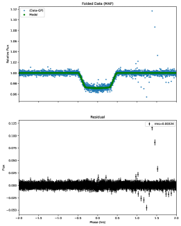
Figure 12: Photometric modelling of TOI-5375. Top: Folded transits in the light curve after the subtraction of the stellar activity signal. The green line shows the best model fit of the transits. Bottom: Residuals of the light curve after the subtraction of the companion transit model.

We performed a search for additional companions by performing a GLS periodogram of the best-fit residuals . The rms of the residuals is very low and no significant additional signals were found. The “best” period is found at $\sim$ 1.97 d (that is, at the stellar rotation period) but with a Scargle power of $\sim$ 3$\times$10^-6, which implies a FAP of 100% (we note that the analytical FAP level of 10% corresponds to a power of 0.0014). This result confirms that our treatment of the stellar activity by means of a SHO kernel does effectively remove it from the light curve. It also shows that if there were more companions in the system, they would be difficult to reveal (at least with the data at hand).

Table 3: Best-fit values obtained for the star-planet model. Photometric fit parameters are from the analysis of the TESS light curve.

Parameter	Prior	Description	Best-fit value
Photometry fit
GP parameters
$\sigma_{\rm GP}$ (e- s-1)	$\mathcal{L}\mathcal{U}$(10-2, 106)	Amplitude of the covariance	0.0876${}_{-0.0002}^{+0.0004}$
$P_{\rm rot}$ (d)	$\mathcal{N}$(1.97,10-2)	Rotation period	1.982${}_{-0.002}^{+0.001}$
$\tau$ (d)	$\mathcal{L}\mathcal{U}$(10-1, 1$0^{4}$)	Time scale of the exponential component	100300${}_{-6}^{+4}$ $\times$ 10-6
White noise terms
$\sigma_{\rm j}$ (e- s-1)	$\mathcal{L}\mathcal{U}$(10-1, 102)	Additional jitter term sector 40	11.16${}_{-0.46}^{+0.31}$ $\times$ 10-5
$\sigma_{\rm j,1}$ (e- s-1)	$\mathcal{L}\mathcal{U}$(10-1, 102)	Additional jitter term sector 47	7.21${}_{-0.16}^{+0.45}$ $\times$ 10-5
$\sigma_{\rm j,2}$ (e- s-1)	$\mathcal{L}\mathcal{U}$(10-1, 102)	Additional jitter term sector 53	13.60${}_{-0.36}^{+0.13}$ $\times$ 10-5
$\sigma_{\rm j,3}$ (e- s-1)	$\mathcal{L}\mathcal{U}$(10-1, 102)	Additional jitter term sector 60	12.29${}_{-0.19}^{+0.24}$ $\times$ 10-5
Companion parameters
$T_{\rm 0}$ (BJD - 2457000 d)	$\mathcal{U}$ (2579, 2582)	Time of inferior conjunction	2580.73564${}_{-0.00005}^{+0.00005}$
$P_{\rm b}$ (d)	$\mathcal{U}$ (1.6, 1.9)	Period	1.721564${}_{0.0000006}^{+0.000004}$
$R_{\rm b}/R_{\star}$	$\mathcal{U}$ (0.0, 0.3)	Companion-to-stellar-radius ratio	0.165${}_{-0.0004}^{+0.0003}$
$a_{\rm b}/R_{\star}$	$\mathcal{U}$ (7, 9)	Semi-major-axis-to-stellar-radius-ratio	8.187${}_{-0.011}^{+0.007}$
$inc$ (degrees)	$\mathcal{U}$ (70, 90)	Orbital inclination	86.38${}_{-0.02}^{+0.02}$
$e$	fixed	Eccentricity	0.00
$c_{\rm 0}$	$\mathcal{U}$ (-1, 1)	Limb-darkening coefficient	0.13${}_{-0.01}^{+0.01}$
Radial velocity fit
White noise term
$\sigma_{\rm j}$ (km s-1)	$\mathcal{L}\mathcal{U}$ (10-3, 103)	Additional jitter	0.29${}_{-0.20}^{+0.29}$
Companion parameters
$\gamma$ (km s-1)	$\mathcal{U}$ (10-3, 103)	RV offset	-61.59${}_{-0.14}^{+0.17}$
$P_{\rm b}$ (d)	$\mathcal{N}$ (1.72,10-7)	Orbital period	1.720${}_{-0.00}^{+0.00}$
$T_{\rm 0,b}$ (MJD, d)	$\mathcal{U}$ (59703.87, 59705.87)	Time of periastron passage	59705.476${}_{-0.004}^{+0.003}$
$K_{\rm b}$ (km s-1)	$\mathcal{U}$ (10-2, 102)	RV semi-amplitude	17.49${}_{-0.22}^{+0.21}$
$e_{\rm b}$	fixed	Orbital eccentricity	0.00
Derived quantities
$M_{\rm b}$ ($M_{\rm J}$)		Mass	77 $\pm$ 8
$R_{\rm b}$ ($R_{\rm J}$)		Radius	0.99 $\pm$ 0.16
$\rho_{\rm b}$ (g cm-3)		Density	98 $\pm$ 49
$a_{\rm b}$ (au)		Semi-major axis	0.0251 $\pm$ 0.0012
Teq,b (K)		Equilibrium temperature	931 - 1107

4.3 Ground-based photometry analysis

We also fit the ground-based photometry dataset obtained from the Asiago observatory. These observations confirm the transit of a companion around TOI-5375 and are additional proof that TOI-5375 b is real and not a false positive due to an BEB. We followed a similar analysis as described in Sect. 4.4, see below, but we did not consider the dilution factor (which defines the total flux that falls into the photometric aperture from contaminants divided by the flux contribution of the target star) and a second-order polynomial trend. We treated the stellar limb-darkening contribution by setting the Sloan $r’$ filter in PyLDTk. From the analysis of the ground-based photometry, we derive a companion-to-stellar-radius ratio, $R_{\rm b}/R_{\star}$, of 0.1850 $\pm$ 0.0012 which is larger than the value derived from the analysis of the TESS dataset, see Fig. 13. This difference can be explained by several reasons. To start with, this effect can be due to the fact that the TESS and ground-based observations are taken at different wavelengths (atmospheres absorb larger at some wavelengths and less at others).

Other explanations can be due to stellar activity. A visual inspection of the individual TESS transits reveals that some of them show “bumps” during the transit that can be related to the presence of stellar spots. In some cases, there are also negative “bumps”, likely due to the occultation of faculae. We also note that the TESS and the Asiago datasets are not simultaneous. To clarify this point we analyse each individual TESS transit as well as the ones observed from the Asiago Observatory. In order to analyse the space and the ground-based photometry in a homogeneous way, we use the TESS SAP light curve using a dilution factor to take into account the possible contamination by nearby stars. In addition, the transit depth is fitted simultaneously to both TESS and Asiago datasets.

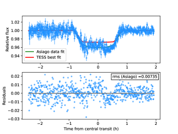
Figure 13: Photometric observations from Asiago, folded on the transit model fit period of TOI-5375 b. Left: October 25th, 2022 observations. Right: December 19th, 2022 observations. The green line shows the best fit to the Asiago dataset, while for comparison purposes we also show in red the best fit derived for the TESS light curves. The residuals of the fit to the Asiago ground-based photometry are shown in the bottom panel.

Figure 14 shows the histogram of the derived $R_{\rm b}/R_{\star}$ for each individual transit. Excluding one clear outlier, the values of $R_{\rm b}/R_{\star}$ obtained from the analysis of the individual TESS transits show a rms of 0.053 covering the range between 0.151 and 0.172. The apparent variation in the companion radius due to the effects of starspots can be written as:

$$\frac{\Delta R}{R}\backsimeq-\frac{1}{2}A_{\lambda}\left(f_{i}-f_{0}\right)$$ (1)

where $A_{\lambda}$ is the contrast which is a function of the bandpass, $f_{0}$ is the filling factor due to un-occulted spots, and $f_{i}$ is the filling factor of spots occulted during the transit. Following Ballerini et al. (2012), for an early-M dwarf like TOI-5375, and taking into account that the TESS passband covers the range from 600 to 1000 nm and is centred on the Cousins $I$-band, we consider $A_{\lambda}$ = 0.924. Then, in the extreme case of $f_{i}$ = 0, we derive a value of $f_{0}$ of the order of 0.285 which is a reasonable value for a very active star like this case. Therefore, we conclude that the spread in $R_{\rm b}/R_{\star}$ from one transit to another can be explained by the stellar activity of the host star. On the other hand, the difference in transit depths between the TESS and the Asiago observations is likely due to a combination of activity and the effect of observing at two different bandpass.

Another possibility could be due to an additional companion (of redder colour) spatially unresolved in Gaia observations. It should be noted that very close binaries ($P$ $<$ 3 days) have very often tertiary companions (Tokovinin et al., 2006). Also, an unresolved companion might explain the slight offset in (V-K) colour with respect to the main sequence. However, this hypothesis is quite speculative, and we do not have indications of an additional component in our spectra.

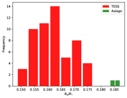
Figure 14: Histogram of the derived $R_{\rm b}/R_{\star}$ values from each individual TESS and Asiago transit.

4.4 Independent joint analysis: TESS and ground-based photometry

In order to have an independent check of our results we perform an additional test by analysing the TESS light curve using the PyORBIT software (Malavolta, 2016; Malavolta et al., 2018) finding similar results. In this case, we analyse the ground-based photometry simultaneously with the TESS data. Furthermore, to test whether or not the difference in transit depth between the Asiago and the TESS data could be due to a possible contamination of the TESS aperture, we used the Simple Aperture Photometry (SAP) fluxes over Presearch Data Conditioning (PDC) ones. In this way, we conserve the contribution of stellar contamination from neighbour stars and later perform our correction for stellar dilution. We followed Mantovan et al. (2022) to calculate the “fraction of light of the stellar PSF which falls into a given photometric aperture” (k parameter) for each star, and we then got the dilution factor (and its associated error).

We selected from the SAP light curves each transit event and an out-of-transit portion twice as long as the transit duration (almost two hours, both before the ingress and after the egress). To perform the selections, we created a mask that flags each transit and cuts portions of the light curves accordingly. For each TESS transit, we fitted the following: the central time of transit ($T_{\rm 0}$), the planetary-to-stellar radius ratio, the impact parameter, b, the stellar density ($\rho_{\star}$, in solar units), the quadratic limb-darkening (LD) law with the parameters q₁ and q₂ introduced in Kipping (2013) - where u₁ and u₂ have been estimated using PyLDTk (Husser et al., 2013; Parviainen et al., 2015) and considering the TESS filter, the dilution factor, a second-order polynomial trend (with c₀ as the intercept, c₁ as the linear coefficient, and c₂ as the quadratic coefficient), and a jitter term (different for each sector, to take into account possible TESS systematics and short-term stellar activity noise) to be added in quadrature to the errors of TESS light curves. We imposed a Gaussian prior on the stellar density, limb-darkening coefficients, and dilution factor, while we kept fixed the period, eccentricity, and argument of pericentre.

We performed a global optimisation of the parameters by running a Differential Evolution algorithm, pyDE (Storn & Price, 1997) and then a Bayesian analysis of each selected light curve around each transit. To perform the latter, we used the affine-invariant ensemble sampler (Goodman & Weare, 2010) for Markov Chain Monte Carlo (MCMC) implemented within the emcee package (Foreman-Mackey et al., 2013). We modelled each transit with batman (Kreidberg, 2015). We fit each transit with $4n_{dim}$ walkers (with $n_{dim}$ being the model’s dimensionality) for 20000 generations with pyDE and then with 300000 steps with emcee – where we applied a thinning factor of 200 to reduce the effect of the chain auto-correlation. We discarded the first 25000 steps (burn-in) after checking the convergence of the chains with the Gelman–Rubin (GR) statistics (Gelman & Rubin, 1992, threshold value R̂ = 1.01). From this analysis, we derive a companion-to-stellar-radius ratio, $R_{\rm b}/R_{\star}$, of 0.1699 $\pm$ 0.0011, similar to the value obtained in the previous analysis ($R_{\rm b}/R_{\star}$, of 0.165 $\pm$ 0.002) . The small difference is likely due to the fact that this time, we analyse the ground-based photometry simultaneously with the TESS data. The best-fitting parameters and the corresponding plots are shown in Appendix  A.

4.5 Search for TTVs and other variability effects

Finally, even though the residuals of the fit of the TESS photometry do not reveal additional signals, a search for Transit Timing Variations (TTVs) due to a possible additional companion orbiting around TOI-5375 was performed (see e.g. Borsato et al., 2019). To this purpose we analyse each individual TESS transit as well as the second transit observed from the Asiago Observatory (the first transit is not included, since, as we have seen, its sampling is not complete). Once the transit times were derived, we fit them with a straight line to obtain a linear ephemeris:

$$T_{\rm 0}=2459604.837650\,(\pm 3\times 10^{-7})$$ (2)

$$+N\times 1.721557\,(\pm 2\times 10^{-6})\,BJD_{TDB}$$ (3)

where $N$ is the epoch of the transit. The corresponding fit is shown in Fig. 15. A search for periodicities in the residuals was performed by means of a GLS periodogram. The periodogram identifies a significant peak at 12.72 $\pm$ 0.03 d with a FAP lower than 1%. The semi-amplitude of the signal is $\sim$ 1 minute. As said, some of the TESS transits are affected by stellar activity. Indeed, according to the simulations performed by Oshagh et al. (2013, Fig. 8), for a transit with $R_{\rm b}/R_{\star}$ $\sim$ 0.15, TTVs of the order of one minute can be explained by the presence of stellar spots with a filling factor of $\sim$ 0.6%. Given the very active nature of TOI-5375, our conclusion is that the $\sim$ 1 minute amplitude TTV signal seen in this star is most likely related to stellar activity. We note that the synodic period between the stellar rotation and the orbital period is 13.59 days, which is close to the apparent TTV period of 12.7 days. This reinforces the interpretation in terms of surface activity features of the apparent TTVs.

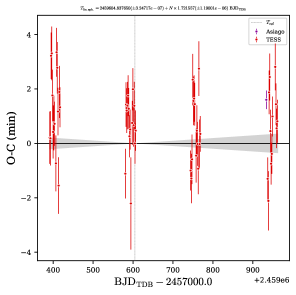
Figure 15: Residuals of the timings of mid-transits versus a linear ephemeris.

Finally, we estimate the photometric flux variations due to other variability effects. In particular, we consider the Doppler beaming (the reflex motion of the star induced by its planetary companion produces Doppler variations in its photometric flux), the ellipsoidal light variations due to tidal effects on the star from the planet as well as the reflected light in the companion surface. Following Loeb & Gaudi (2003) we derive flux variations, $\Delta F/F_{\rm 0}$, of the order of 2.8 $\times$ 10^-4, 9.4 $\times$ 10^-5, and 2.4 $\times$ 10^-4 for Doppler beaming, ellipsodial light variations, and reflected light, respectively. The calculation of Doppler beaming was done in the TESS band ($\lambda$ $\sim$ 7850 Å), while for the reflected light effect a geometric albedo of 2/3 was considered. All these effects are extremely small compared with the intrinsic variability of the star (the TESS light curve shows a rms of 26.7, 54.35, 68.68, and 43.96 e^- s^-1 in Sectors 40, 47, 53 and 60, respectively).

4.6 High energy events in the TESS light curve

Many energetic events or flares seem to be present in the TESS light curve (see Fig. 1). This is in agreement with the high rotation level of this star but it might also be evidence of a possible interaction between TOI-5375 and its companion. In order to test this hypothesis we use the methodology described by Colombo et al. (2022) to identify the impulsive events and derive their amplitudes and the amount of energy emitted. We then phase-fold the times at which the events take place with the companion period (1.72 d), the rotation period (1.97 d) as well as the synodic period of the TOI-5375 system. The synodic period is defined as $1/P_{\rm synodic}=1/P_{\rm companion}-1/P_{\rm rotation}$, that is, P_synodic = 13.59 d. Figure 16 shows the number of events (blue empty histogram) and the released energy (orange filled histogram) phase-folded with the companion period (left) and with the synodic period (centre), and the stellar period (right). In order to test whether the distribution of the released energy is or not uniform we made use of a Kolmogorov-Smirnov (KS) test . The results are shown in Table 4. In all cases, we test the null hypothesis that the phase-folded released energy distribution is drawn from a uniform distribution. The results from the K-S test show that the distribution of events is far from uniform which supports the star-companion interaction scenario. When phased to the stellar rotation period, four main peaks of events can be seen at phases $\sim$ 0.1, 0.4, 0.7 and $\sim$ 0.9. The first peak is driven by an energetic event in Sector 53 (see Fig. 1, green square). The peak at phase $\sim$ 0.4 corresponds to an energetic event in Sector 47 (shown as a purple triangle in Fig. 1), which is followed by many more, less energetic, events. The peak at phase $\sim$ 0.7 is driven by two high-energetic events in Sectors 60 and 53 (marked with a red diamond and a red circle in Fig. 1), again followed by several less energetic events. Finally, it can be seen a fourth peak close to a phase 0.9 corresponding to a high-energy event in Sector 40 (see Fig. 1, red circle). On the other hand, if the distribution of events is folded with respect to the period of the orbital companion (Fig. 16, left) or the synodic period (Fig. 16, centre), the impulsive events are mainly at phase values between 0.0 and 0.6 and are driven by the five energetic events already discussed.

Table 4: Results of the K-S tests performed in this work.

Distribution phase-folded to	K-S statistic	$p$-value	H${}^{{\ddagger}}_{\rm 0}$
Companion’s orbital period (1.72 d)	0.74	4.30 $\times$ 10-11	1
System’s synodic period (13.59 d)	0.68	2.30 $\times$ 10-9	1
Stellar rotation period (1.97 d)	0.89	5.30 $\times$ 10-19	1

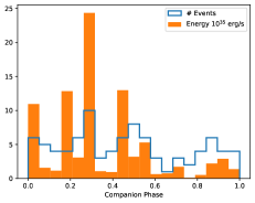
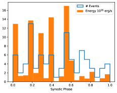
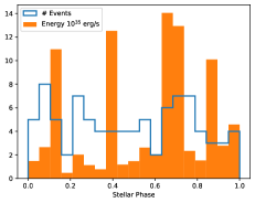
Figure 16: Histogram of impulsive events (blue empty line) and amount of energy emitted (orange filled histogram) phase-folded to the companion orbital period (left), the synodic period (centre) and the stellar period (right).

4.7 RV time series analysis

Table 5 provides the RVs time series for TOI-5375 analysed in this work which, as discussed earlier, are those obtained by the LSD method. The RV data show a rms of 12.42 km s^-1, which is approximately 35 times the mean error of the measured RVs (0.36 km s^-1). The GLS periodogram (see Fig. 17) reveals a double peak structure with significant frequencies at f₁ = 0.4202 $\pm$ 0.0008 d^-1 (P = 2.380 $\pm$ 0.004 d), and f₂ = 0.5810 $\pm$ 0.0006 d^-1 (P = 1.721 $\pm$ 0.002 d). For frequencies values larger than 0.5 d^-1 the periodogram is clearly a mirror copy of the one between 0 and 0.5 d^-1 so both peaks should be related. The significance of these frequencies was tested by using a bootstrapping analysis to compute the FAPs values (see e.g. Endl et al., 2001). The signal at 1.72 d agrees well with the periodicity found for the transit of TOI-5375 b in the light curve analysis. On the other hand, the period at 2.38 d is likely due to the observing sampling as our observations have a gap of $\sim$ 6 d (—f₁ - f₂— $\sim$ 1/6 d^-1).

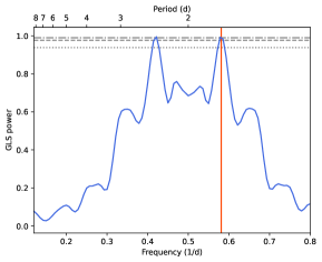
Figure 17: GLS periodogram of the RV dataset. Values corresponding to a FAP of 10, 1, and 0.1% are shown with horizontal grey lines. The vertical line indicates the period of TOI-5375 b at 1.72 d.

Table 5: RVs (with their corresponding uncertainties) of TOI-5375 used in this work.

MJD	RV	$\Delta$RV
(d)	(km s-1)	(km s-1)
59703.87173611112	-46.37	0.42
59705.87925925944	-59.28	0.33
59706.89432870364	-52.57	0.45
59707.880509259645	-75.41	0.82
59713.876840277575	-48.67	0.36
59714.874594907276	-78.84	0.33
59715.87714120373	-44.97	0.18
59716.87711805524	-73.85	0.17
59717.86982638901	-56.77	0.15

We have applied the same Bayesian framework as for the photometric curve to the RV data but, in this case, the model contains only a Keplerian signal and the number of live points has been set to 2000. Given the small number of RVs points, we do not perform a simultaneous analysis of the RV with the photometry. Instead, we take advantage of the photometry fit and set tight priors in the RV fitting on all parameters but in K_b, where a wide prior was considered, see Table 3. The resulting posterior distributions are shown in Fig. 18 while Fig. 19 shows the best-fit planet model (top) and the corresponding RV residuals (bottom). The best-fit parameters are also listed in Table 3. No significant signals are found in the analysis of the RV residuals. We note that the resiudals show a larger dispersion during the first observing season. A possible explanation for this could be related to the high variability and activity level of TOI-5375.

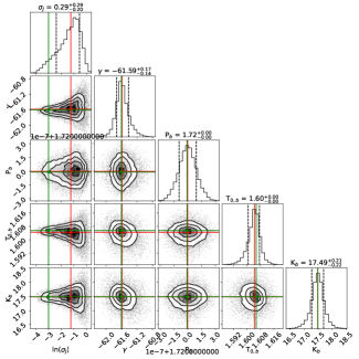
Figure 18: Posterior distributions of the Bayesian fit of the RVs.

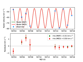
Figure 19: Best-fit planetary model for TOI-5375 b (top), and RV residuals (bottom).

For the sake of completeness, we also measured the main activity indexes of chromospheric activity, namely the Ca ii H & K index, H$\alpha$, and Na i D₁, D₂ (see e.g. Maldonado et al., 2019). All indexes show a symmetric periodogram around 0.5 d^-1 with several peaks, all with a significance below the 10% analytical FAP value. Only the H$\alpha$ index shows a dominant peak, close to the rotation period at $\sim$ 1.99 d. The time series of the different activity indexes as well as their corresponding periodograms are shown in Appendix B.

5 Discussion

From the best values of $K_{\rm b}$ and $P_{\rm b}$ derived in the previous section, we derived a mass for TOI-5375 b of 77 $\pm$ 8 ($M_{\rm J}$) and a semi-major axis $a$ = 0.0251 $\pm$ 0.0012 au. On the other hand, from the analysis of the light curve, we obtain a radius of 0.99 $\pm$ 0.16 ($R_{\rm J}$). TOI-5375 b is therefore an object in the boundary between the brown dwarfs and the very-low-mass stars. This is a remarkable result, as massive substellar companions orbiting around M dwarfs are rare (see Sect. 1). Figure 20 shows the position of TOI-5375 b in the planetary radius versus planetary mass diagram. For comparison purposes, the location of the known substellar companions around late-K and M dwarf stars (with known values of planetary radius and mass) are shown. In order to discuss our results in a broader context, we also show the location of several known brown dwarfs and low-mass stars orbiting around a late-K or M dwarf primary (Mireles et al., 2020; Carmichael, 2022).

The figure shows two regimes of the mass-radius relationship. Up to planetary masses of the order of $\sim$ 0.2 $M_{\rm J}$, the planetary radius steadily increases with the planetary mass. For higher masses, the radius remains constant and even shows a slight decrease with increasing planetary mass. TOI-5375 b is clearly located in the region of the diagram where $R_{\rm p}$ is roughly constant ($\sim$ 1 $R_{\rm J}$) with $M_{\rm p}$. The two regimes of the mass-radius relationship are related to the boundary between objects with a dominating hydrogen and helium composition and objects that consist of different composition and different mass-radius relationships (see e.g. Bashi et al., 2017, and references therein).

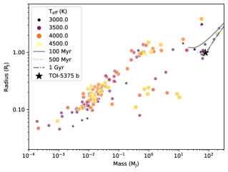
Figure 20: Known substellar companions and low-mass stars (radius versus mass) around late-K and M dwarfs (As listed at http://exoplanet.eu/). Different colours and symbol sizes indicate the effective temperature of the host star. Models for substellar objects and low-mass stars with solar metallicity from Baraffe et al. (2015) are overplotted with grey lines.

The TOI-5375 system constitutes an interesting case study that can help us to shed light on the tidal interactions between close companions and their host stars. With an orbital period for TOI-5375 b of 1.72 d, a rotational period for the host star of 1.97 d, the system is likely being observed in the short time frame in which the star is close to synchronising its rotation with the orbital period of the companion. Tidally driven orbital circularisation and synchronisation is a well-known phenomenon in binary systems containing low-mass stars (e.g. Zahn & Bouchet, 1989), whilst the evidence for similar phenomena in systems harbouring short period hot Jupiter planets have been recently discussed (Birkby et al., 2014; Maciejewski et al., 2016; Patra et al., 2017; Wilkins et al., 2017; Bouma et al., 2019; Yee et al., 2020).

Taking into account the properties of the TOI-5375 system, tidal dissipation should be mainly driven by inertial waves (Ogilvie & Lin, 2007). Under these circumstances, and following the model described in Barker (2020), we derive a tidal quality factor due to inertial waves of $Q^{\prime}_{\rm IW}$ = 3.9 $\times$ 10⁵. We use the formulae of Leconte et al. (2010) which takes into account the rotation of the star in the evolution of the system parameters to derive the characteristic time-scales (the e-folding time $\tau$ of a given parameter $q$ is defined as $\frac{1}{\tau}=\frac{1}{q}\frac{dq}{dt}$) for the TOI-5375 system. We derive an estimated time-scale for tidal synchronisation of the stellar spin of only $\sim$ 3.36 Myr and a circularisation time-scale of $\sim$ 6.76 Myr. Such a synchronisation timescale is much shorter than the angular momentum loss timescale of the stellar magnetised wind (of the order of 100 Myr given the fast rotation of the star), thus supporting the statement of Sect. 3.1 that we cannot use gyrochronology to estimate the age of this star. As a matter of fact, the rotation period of TOI-5375 is expected to be longer than about 10 days from the central plot in Fig. 6, given that it is likely to belong to the thin disk stars, that is, it is probably older than the Hyades. Conversely, it shows a rotation period as short as 1.97 days that we interpret as the consequence of the tidal acceleration given an estimated present synchronisation timescale much shorter than the expected magnetic braking timescale. The characteristic time-scale for the semi-major axis decay is $\sim$ 115 Myr, while the obliquity of the orbit has a decay time-scale of $\sim$ 0.72 Myr. The total angular momentum of the system is about 1.61 times larger than the minimum value required to reach a final stable tidal equilibrium with the star and the low-mass companion fully synchronised on a circular orbit. After that stage, the orbit will slowly decay as a result of the angular momentum losses in the magnetised stellar wind of the star (see Damiani & Lanza, 2015).

Given the mass ratio between the star and its companion, $M_{\star}$ / $M_{\rm b}$ $\sim$ 8.7, it is likely that the TOI-5375 system was formed as a low-mass binary system. One possibility is that TOI-5375 and its companion formed from the same molecular cloud that fragmented into two objects. Another possibility is that TOI-5375 formed a protoplanetary disc susceptible to gravitational instabilities. A relationship between the disc mass and the stellar mass of the form $M_{\rm disc}$ $\propto$ $M_{\star}^{\rm 1.2}$ has been suggested (Alibert et al., 2011). Thus, the relatively low-mass protoplanetary disc around an M dwarf star like TOI-5375 avoided the formation of two stellar objects of equal mass. Disc fragmentation has been shown to successfully explain the formation of relatively close binaries, and due to the interactions with their natal disc, significant migration can also occur (e.g. Kratter, 2011). Simulations show that discs with a moderate size and mass (100 au, 0.25 $M_{\odot}$) might fragment around late-K/early-M dwarfs forming mainly brown dwarfs, but also low-mass hydrogen-burning stars in generally close-in orbits (Stamatellos et al., 2011). Therefore, another piece of evidence supporting the disc fragmentation might come from the fact that TOI-5375 and its companion are very close and the star is to align its stellar spin with the binary orbit. However, we should note that the current spin-orbit alignment of the star may not be primordial, but it could have been established recently because the present timescale for the obliquity damping by tides is only 0.72 Myr (see above).

6 Conclusions

In this work, we report the discovery and confirmation of a transiting companion in the brown dwarf / very-low-mass star boundary, TOI-5375 b, orbiting an active M0.5 dwarf with a period of 1.72 d. We make use of the available TESS photometric data and high-resolution HARPS-N spectra to model the signals present in the data. We derive a rotational period of 1.97 d for the host star and conclude that the orbit of the companion decays quickly and that the system should be in the phase in which the star is very close to synchronising its rotation with the orbital period of the companion.

TOI-5375 b, with a mass of 77 $\pm$ 8 $M_{\rm J}$ and a radius of 0.99 $\pm$ 0.16 $R_{\rm J}$, joins the population of massive substellar / low-mass stellar companions in close-in orbits around low-mass stars that is currently emerging. Further studies of the properties of these objects will help us to explore our models of low-mass companion formation and migration as well as to study how the tidal interactions with their host stars affect their evolution.

We can measure the change in the orbit of TOI-5375 b by computing the associated shift in transit arrival time (transits should occur earlier as the companion’s orbit decay). We obtain a shift in the transit time of 20.53 seconds in a timespan of 10 yr. In our analysis, we have combined data from four TESS sectors containing a total of 53 transits. The precision in the estimated transit-mid time (from the simultaneous analysis of all transits) is of the order of 5$\times$10^-5 d or $\sim$ 4.32 s, while the relative error in the transit’s depth is of the order of $\sim$0.2%. Therefore, while TOI-5375 is a good candidate to observe transit timing variations due to the effects of tidal waves, a long-term monitoring observation from ground-based facilities of this star would be needed (unfortunately the star is too faint to be observed by the CHEOPS satellite).

The TOI-5375 system can also be an interesting target for ongoing and future space missions aimed at the characterisation of the atmospheres of substellar companions like the James Webb Space Telescope (Gardner et al., 2006) or Ariel (Tinetti et al., 2018). We computed the transmission spectroscopy metric (TSM) as well as the emission spectroscopy metric (ESM) following the procedure defined in (Kempton et al., 2018). The derived TSM value, 0.94, is significantly low, but we caution that TSM values were defined for small, rocky planets, so it is unclear whether or not they are still valid for a massive brown dwarf like TOI-5375 b or not. On the other hand, we obtain an ESM value of 125, which suggests that TOI-5375 b is indeed a good target for atmospheric characterisation.

In order to test what we might expect in the future, we generate a synthetic spectrum of TOI-5375 b as observed by Ariel. For this purpose, we made use of a PHOENIX/BT-SETTL atmospheric model (Allard et al., 2012) with parameters T_eff = 1000 K, $\log g$ = 4.5 cm s^-2, and [Fe/H] = +0.00 dex. We convolved the original model with a Gaussian filter in order to match the expected resolution for Ariel Tier 2 observations (R $\sim$ 50 at 1.95 - 3.95 $\mu$m) and computed the expected fluxes at Ariel wavelengths. The synthetic spectrum is shown in Fig. 21. The comparison of the spectral properties of TOI-5375 b with other brown dwarfs and stars will help us to discover whether their atmospheric properties are equal or deviating, which may be a signspot for different formation scenarios.

We acknowledge that while this manuscript was under the referee review process, an independent analysis of the TOI-5375 system has been published (Lambert et al., 2023). These authors found similar results to ours. Nevertheless, we have intentionally maintained our analysis completely independent of these authors.

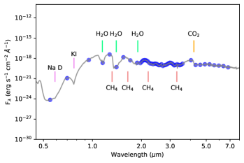
Figure 21: Simulated observed spectrum by the Ariel mission of TOI-5375 b generated from a PHOENIX/BT-SETTL atmospheric model. The grey line shows the spectra degraded to a resolution of R = 50, while the blue circles indicate the expected fluxes at Ariel wavelengths. Some characteristic spectral features of a brown dwarf are indicated (see e.g. Burrows et al., 2002; Burgasser et al., 2006; Sorahana & Yamamura, 2012).

Appendix A Results from the joint analysis: TESS and ground-based photometry

Table 6 provides the best-fit values obtained for the simultaneous fit of the TESS SAP light curve and the Asiago observations, as described in Sect. 4.4. The best transit model fit is shown in Figure 22.

Table 6: Best-fit values obtained for the simultaneous fit of the TESS SAP light curve and the Asiago observations.

Parameter	Description	Best-fit value
$\sigma_{\rm ground,1}$	Jitter Asiago dataset 1	0.0040${}_{-0.0002}^{+0.0002}$
$R_{\rm b}/R_{\star}$,Ground 1	Companion-to-stellar-radius ratio, Asiago data 1	0.191${}_{-0.002}^{+0.002}$
$\sigma_{\rm ground,2}$	Jitter Asiago dataset 2	0.0040${}_{-0.0003}^{+0.0003}$
$R_{\rm b}/R_{\star}$,Ground 2	Companion-to-stellar-radius ratio, Asiago data 2	0.188${}_{-0.002}^{+0.002}$
$\sigma_{\rm 0}$	TESS jitter term sector 40	0.76${}_{-0.51}^{+0.56}$
$\sigma_{\rm 1}$	TESS jitter term sector 50	6.11${}_{-0.12}^{+0.12}$
$\sigma_{\rm 2}$	TESS jitter term sector 53	0.86${}_{-0.54}^{+0.48}$
$\sigma_{\rm 3}$	TESS jitter term sector 60	2.07${}_{-0.29}^{+0.26}$
$P_{\rm b}$ (d)	Period	1.721556${}_{-0.000001}^{+0.000001}$
$b$	Impact parameter	0.43${}_{-0.03}^{+0.02}$
$T_{\rm 0}$ (BJD, d)	Time of inferior conjunction	2459580.736510${}_{-0.000096}^{+0.000095}$
$R_{\rm b}/R_{\star}$,TESS	Companion-to-stellar-radius ratio, TESS	0.170${}_{-0.001}^{+0.001}$
$\rho_{\star}$ ($\rho_{\odot}$)	Stellar density	2.57${}_{-0.09}^{+0.09}$
$c_{\rm 1}$, TESS	Limb-darkening coefficient TESS	0.21${}_{-0.05}^{+0.06}$
$c_{\rm 2}$, TESS	Limb-darkening coefficient TESS	0.35${}_{-0.06}^{+0.07}$
$c_{\rm 1}$, Ground	Limb-darkening coefficient Asiago	0.42${}_{-0.07}^{+0.08}$
$c_{\rm 2}$, Ground	Limb-darkening coefficient Asiago	0.35${}_{-0.03}^{+0.04}$
$d$, TESS	Dilution factor TESS	0.0756${}_{-0.0005}^{+0.0005}$
$a_{\rm b}/R_{\star}$	Semi-major-axis-to-stellar-radius-ratio	8.28${}_{-0.09}^{+0.09}$
$inc$ (degrees)	Orbital inclination	87.00${}_{-0.21}^{+0.22}$
$R_{\rm b}$ ($R_{\rm J}$)	Companion Radius	1.05${}_{-0.03}^{+0.03}$
$a_{\rm b}$ (au)	Companion Semi-major axis	0.024${}_{-0.008}^{+0.001}$

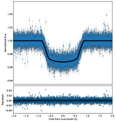
Figure 22: Photometric modelling of TOI-5375 (TESS and Asiago photometry). Top: Folded transits in the light curve after the subtraction of the stellar activity signal. The black line shows the best model fit of the transits. Bottom: Residuals of the light curve after the subtraction of the companion transit model.

Appendix B Activity indexes

Figure 23 shows the temporal variation of the different activity indexes measured in this work, while the periodogram analysis is given in Fig. 24. Table 7 provides the measured values with their corresponding uncertainties.

Table 7: Activity indexes measured for TOI-5375.

MJD (d)	Ca ii H & K	H$\alpha$	Na i
59703.871736	4.9593 $\pm$ 5.1386	1.1264 $\pm$ 0.0145	0.4049 $\pm$ 0.0082
59705.879259	4.3944 $\pm$ 2.9213	1.0575 $\pm$ 0.0122	0.3679 $\pm$ 0.0058
59706.894329	2.9384 $\pm$ 2.1017	0.8998 $\pm$ 0.0093	0.3147 $\pm$ 0.0048
59707.880509	2.8771 $\pm$ 1.5704	1.0925 $\pm$ 0.0144	0.3926 $\pm$ 0.0090
59713.876840	3.2140 $\pm$ 0.9153	1.1185 $\pm$ 0.0080	0.3907 $\pm$ 0.0041
59714.874595	2.4812 $\pm$ 1.0379	1.1102 $\pm$ 0.0148	0.4731 $\pm$ 0.0083
59715.877141	4.3896 $\pm$ 1.3210	1.1187 $\pm$ 0.0067	0.3913 $\pm$ 0.0032
59716.877118	4.5392 $\pm$ 1.5677	0.9172 $\pm$ 0.0042	0.3126 $\pm$ 0.0023
59717.869826	4.2266 $\pm$ 1.3254	1.0776 $\pm$ 0.0071	0.3711 $\pm$ 0.0032

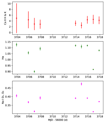
Figure 23: From top to bottom: Ca ii H & K index, H$\alpha$ index, and Na i D₁, D₂ index time series for TOI-5375.

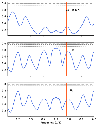
Figure 24: From top to bottom: GLS periodogram of the Ca ii H & K, H$\alpha$, and Na i activity indexes. The vertical line indicates the period of TOI-5375 b at 1.72 d. Values corresponding to a FAP of 10%, 1%, and 0.1% are shown with horizontal grey lines.