Note on the Time Dilation of Charged Quantum Clocks

Abstract

We derive the time dilation formula for charged quantum clocks in electromagnetic fields. As a concrete example of non-inertial motion, we consider a cyclotron motion in a uniform magnetic field. Applying the time dilation formula to coherent state of the charged quantum clock, we evaluate the time dilation quantum-mechanically.

I Introduction

Motivated by the tests of the weak equivalence principle in quantum regime, in our previous study we derived a formula of the averaged proper time read by one clock conditioned on another clock reading a different proper time in a weak gravitational field Chiba and Kinoshita (2022) by extending the proper time observable proposed in Smith and Ahmadi (2020). The time dilation measured by these quantum clocks is found to have the same form as that in classical relativity. There, clocks are assumed to be in their inertial motion and their classical trajectories are the geodesics of the spacetime, that is, the clocks are always free-falling.

Then, it would also be interesting to study what would happen for clocks in non-inertial motion. Any non-inertial motion should be caused by other external force than gravitational interaction, and it is not a priori clear whether the formalism in Smith and Ahmadi (2020) can be extended to such situations. In classical relativity, we are allowed to assume a non-inertial trajectory without the equation of motion, so that we can evaluate its proper time kinematically. On the other hand, in quantum theory we need to solve quantum dynamics to determine a trajectory.

In order to study the effect of non-inertial motion on the time dilation of quantum clocks, we consider charged quantum clocks interacting with the external electromagnetic fields as a concrete example. The study of a quantum charged particle is also interesting in the light of quantum mechanics in a rotating frame because there exists a close analogy between the motion in a rotating frame and the motion in a magnetic field Sakurai (1980). Also, a new class of optical clocks with highly charged ions has been received interest in recent years as references for highest-accuracy clocks and precision tests of fundamental physics Kozlov et al. (2018); King et al. (2022). Such an optical clock based on a highly charged ion was recently realized King et al. (2022). Our study may be applicable to such clocks.

The paper is organized as follows. In Sec. II, we derive the time dilation formula for charged particles in electromagnetic fields and weak gravitational fields as the average of a proper time observable for a quantum clock. We extend the formalism given in Smith and Ahmadi (2020) to include the shift vector as well as the electromagnetic field which is essential to treat a rotational motion and a rotating frame. In Sec. III, as a non-inertial motion, we consider the cyclotron motion in a uniform magnetic field. We evaluate the quantum time dilation by using the coherent state. In Appendix A, we summarize the several results of the coherent state for the cyclotron motion in quantum mechanics and the discussion of the time dilation in a rotating frame.

II Charged Quantum Clock Particles in Spacetime

II.1 Classical Particles

We consider a system of $N$ charged massive particles. Each particle whose mass and charge are $m_{n}$ and $q_{n}~{}(n=1,\dots,N)$ has a set of internal degrees of freedom, labeled by the configuration variables $\chi_{n}$ and their conjugate momenta $P_{\chi_{n}}$Smith and Ahmadi (2020). These internal degrees of freedom are supposed to represent the quantum clock.

The action of such a system in a curved spacetime with the metric $g_{\mu\nu}$ and an electromagnetic field $A_{\mu}$ is given by

$$S=\sum_{n}\int d\tau_{n}\left(-m_{n}c^{2}+q_{n}A_{\mu}\frac{dx_{n}^{\mu}}{d\tau_{n}}+P_{\chi_{n}}\frac{d\chi_{n}}{d\tau_{n}}-H_{n}^{\rm clock}\right),$$ (1)

where $\tau_{n}$ is the proper time of the $n$th particle and $H_{n}^{\rm clock}=H_{n}^{\rm clock}(\chi_{n},P_{\chi_{n}})$ is a Hamiltonian for its internal degrees of freedom.

Let $x_{n}^{\mu}$ denote the spacetime position of the $n$th particle. The trajectory of the $n$th particle $x_{n}^{\mu}(t)$ is parameterized by an arbitrary external time parameter $t$. Noting that $cd\tau_{n}=\sqrt{-g_{\mu\nu}\dot{x}_{n}^{\mu}\dot{x}_{n}^{\nu}}dt\equiv\sqrt{-\dot{x}^{2}_{n}}dt$, where a dot denotes differentiation with respect to $t$, the action is rewritten as

$$S=\int dt\sum_{n}\frac{1}{c}\sqrt{-\dot{x}_{n}^{2}}\left(-m_{n}c^{2}+q_{n}A_{\mu}\frac{\dot{x}_{n}^{\mu}c}{\sqrt{-\dot{x}_{n}^{2}}}+P_{\chi_{n}}\frac{\dot{\chi}_{n}c}{\sqrt{-\dot{x}_{n}^{2}}}-H_{n}^{\rm clock}\right)=:\int dt~{}L.$$ (2)

The momentum conjugate to $x_{n}^{\mu}$ is given by

$$P_{n\mu}=\frac{\partial L}{\partial\dot{x}_{n}^{\mu}}=\frac{g_{\mu\nu}\dot{x}_{n}^{\nu}}{c\sqrt{-\dot{x}_{n}^{2}}}\left(m_{n}c^{2}+H_{n}^{\rm clock}\right)+q_{n}A_{\mu}.$$ (3)

Then the Hamiltonian associated with the Lagrangian $L$ is constrained to vanish:

$$H=\sum_{n}\left(P_{n\mu}\dot{x}_{n}^{\mu}+P_{\chi_{n}}\dot{\chi}_{n}\right)-L\approx 0.$$ (4)

In terms of the momentum, the constraints can be expressed in the form

$$C_{H_{n}}:=g^{\mu\nu}(P_{n\mu}-q_{n}A_{\mu})(P_{n\nu}-q_{n}A_{\nu})c^{2}+\left(m_{n}c^{2}+H_{n}^{\rm clock}\right)^{2}\approx 0.$$ (5)

Using the $(3+1)$ decomposition of the metric in terms of the lapse function $\alpha$, the shift vector $\beta^{i}$ and the three-metric $\gamma_{ij}$ such that Misner et al. (2017)

$$ds^{2}=-\alpha^{2}c^{2}dt^{2}+\gamma_{ij}(dx^{i}+\beta^{i}cdt)(dx^{j}+\beta^{j}cdt),$$ (6)

the constraint is factorized in the form

$$C_{H_{n}} = -\alpha^{-2}\left(P_{n0}-q_{n}A_{0}-\beta^{i}\left(P_{ni}-q_{n}A_{i}\right)\right)^{2}c^{2}+\gamma^{ij}(P_{ni}-q_{n}A_{i})(P_{nj}-q_{n}A_{j})c^{2}+\left(m_{n}c^{2}+H_{n}^{\rm clock}\right)^{2}$$ (7)

$$= -\alpha^{-2}C_{n}^{+}C_{n}^{-}\approx 0,$$

where $C_{n}^{\pm}$ is defined by

$$C_{n}^{\pm} := \left(P_{n0}-q_{n}A_{0}-\beta^{i}\left(P_{ni}-q_{n}A_{i}\right)\right)c\pm h_{n},$$ (8)

$$h_{n} := \alpha\sqrt{\gamma^{ij}(P_{ni}-q_{n}A_{i})(P_{nj}-q_{n}A_{j})c^{2}+(m_{n}c^{2}+H_{n}^{\rm clock})^{2}}.$$ (9)

Note that we have set $x^{0}=ct$. Hereafter we assume that the spacetime is stationary. The coordinates $x^{\mu}_{n}$ and their conjugate momenta $P_{n\mu}$ satisfy the fundamental Poisson brackets: $\{x_{m}^{\mu},P_{n\nu}\}=\delta_{mn}\delta^{\mu}_{\nu}$. The canonical momentum $P_{n\mu}$ generates translations in the spacetime coordinate $x_{n}^{\mu}$. Therefore, if $C_{n}^{\pm}\approx 0$, then $\pm h_{n}-q_{n}A_{0}c-\beta^{i}c\left(P_{ni}-q_{n}A_{i}\right)$ is the generator of translation in the $n$th particle’s time coordinate and is the Hamiltonian for both the external and internal degrees of freedom of the $n$th particle.

II.2 Quantization

We canonically quantize the system of $N$ particles by promoting the phase space variables to operators acting on appropriate Hilbert spaces: $x^{0}_{n}$ and $P_{n0}$ become canonically conjugate self-adjoint operators acting on the Hilbert space ${\cal H}^{0}_{n}\simeq L^{2}(\mathbb{R})$ associated with the $n$th particle’s temporal degree of freedom; operators $x_{n}^{i}$ and $P_{ni}$ acting on the Hilbert space ${\cal H}_{n}^{\rm ext}\simeq L^{2}(\mathbb{R}^{3})$ associated with the particle’s external degrees of freedom; operators $\chi_{n}$ and $P_{\chi_{n}}$ acting on the Hilbert space ${\cal H}_{n}^{\rm clock}$ associated with the particle’s internal degrees of freedom. Then the Hilbert space describing the $n$th particle is ${\cal H}_{n}\simeq{\cal H}^{0}_{n}\otimes{\cal H}_{n}^{\rm ext}\otimes{\cal H}_{n}^{\rm clock}$.

The constraint equations (7) now become operator equations restricting the physical state of the theory,

$$C_{n}^{+}C_{n}^{-}|\Psi\rangle\rangle=0,~{}~{}~{}~{}\forall n,$$ (10)

where $|\Psi\rangle\rangle\in{\cal H}_{\rm phys}$ is a physical state of a clock $C$ and a system $S$ and lives in the physical Hilbert space ${\cal H}_{\rm phys}$.

To specify ${\cal H}_{\rm phys}$, the normalization of the physical state in ${\cal H}_{\rm phys}$ is performed by projecting a physical state $|\Psi\rangle\rangle$ onto a subspace in which the temporal degree of freedom of each particle (clock $C$) is in an eigenstate $|t_{n}\rangle$ of the operator $x_{n}^{0}$ associated with the eigenvalue $t\in\mathbb{R}$ in the spectrum of $x_{n}^{0}$: $x_{n}^{0}|t_{n}\rangle=ct|t_{n}\rangle$. The state of $S$ by conditioning $|\Psi\rangle\rangle$ on $C$ reading the time $t$ is then given by

$$|\psi_{S}(t)\rangle=\langle t|\otimes I_{S}|\Psi\rangle\rangle,$$ (11)

where $|t\rangle=\otimes_{n}|t_{n}\rangle$ and $I_{S}$ is the identity on ${\cal H}\simeq\bigotimes_{n}{\cal H}_{n}^{\rm ext}\otimes{\cal H}_{n}^{\rm clock}$. We demand that the state $|\psi_{S}(t)\rangle$ is normalized as $\langle\psi_{S}(t)|\psi_{S}(t)\rangle=1$ for $\forall t\in\mathbb{R}$ on a spacelike hypersurface defined by all $N$ particles’ temporal degree of freedom being in the state $|t_{n}\rangle$. The physical state $|\Psi\rangle\rangle$ is thus normalized with respect to the inner product Smith and Ahmadi (2020):

$$\langle\langle\Psi|\Psi\rangle\rangle_{PW}:=\langle\langle\Psi||t\rangle\langle t|\otimes I_{S}|\Psi\rangle\rangle=\langle\psi_{S}(t)|\psi_{S}(t)\rangle=1,$$ (12)

and the physical state $|\Psi\rangle\rangle$ can be written as

$$|\Psi\rangle\rangle=\int dt|t\rangle\langle t|\otimes I_{S}|\Psi\rangle\rangle=\int dt|t\rangle|\psi_{S}(t)\rangle.$$ (13)

Hereafter, we consider physical states that satisfy $C_{n}^{+}|\Psi\rangle\rangle=0$ for all $n\in\mathbb{N}$. It can be shown that the conditioned state $|\psi_{S}(t)\rangle$ satisfies the Schrödinger equation with $t$ as a time parameter Smith and Ahmadi (2020):

$$i\hbar\frac{d}{dt}|\psi_{S}(t)\rangle=H_{S}|\psi_{S}(t)\rangle,$$ (14)

where $H_{S}$ is given by

$$H_{S}=\sum_{n}\left(h_{n}-q_{n}A_{0}c-\beta^{i}c\left(P_{ni}-q_{n}A_{i}\right)\right)\otimes I_{S-n}\equiv\sum_{n}\widetilde{h_{n}}\otimes I_{S-n}$$ (15)

with $I_{S-n}$ being the identity on $\bigotimes_{m\neq n}{\cal H}^{\rm ext}_{m}\otimes{\cal H}^{\rm clock}_{m}$. Therefore, $|\psi_{S}(t)\rangle$ can be regarded as the time-dependent state of the $N$-particles with the Hamiltonian $H_{S}$ evolved with the external time $t$.

II.3 Probabilistic Time Dilation

Consider two clock particles $\mathrm{A}$ and $\mathrm{B}$ with internal degrees of freedom. Each clock is defined to be the quadrupole $\{{\cal H}^{\rm clock}_{n},\rho_{n},H^{\rm clock}_{n},T_{n}\}$, where $\rho_{n}$ is a fiducial state and $T_{n}$ is proper time observable for $n\in\{\mathrm{A},\mathrm{B}\}$. The proper time observable is defined as a POVM (positive operator valued measure)

$$T_{n}:=\left\{E_{n}(\tau)~{}\forall\tau\in G~{}{\rm s.t.}\int_{G}d\tau E_{n}(\tau)=I_{n}\right\},$$ (16)

where $E_{n}(\tau)=|\tau\rangle\langle\tau|$ is a positive operator on ${\cal H}^{\rm clock}_{n}$, $G$ is the group generated by $H^{\rm clock}_{n}$, and $|\tau\rangle$ is a clock state associated with a measurement of the clock yielding the time $\tau$.

To probe time dilation effects between two clocks, we consider the probability that clock $\mathrm{A}$ reads the proper time $\tau_{\mathrm{A}}$ conditioned on clock $\mathrm{B}$ reading the proper time $\tau_{\mathrm{B}}$ Page and Wootters (1983); Wootters (1984). This conditional probability is given in terms of the physical state as

$${\rm Prob}[T_{\mathrm{A}}=\tau_{\mathrm{A}}|T_{\mathrm{B}}=\tau_{\mathrm{B}}]=\frac{\langle\langle\Psi|E_{\mathrm{A}}(\tau_{\mathrm{A}})E_{\mathrm{B}}(\tau_{\mathrm{B}})|\Psi\rangle\rangle}{\langle\langle\Psi|E_{\mathrm{B}}(\tau_{\mathrm{B}})|\Psi\rangle\rangle}\,.$$ (17)

Consider the case where two clock particles $\mathrm{A}$ and $\mathrm{B}$ are moving in a curved spacetime. Suppose that initial conditioned state is unentangled, $|\psi_{S}(0)\rangle=|\psi_{S_{\mathrm{A}}}\rangle|\psi_{S_{\mathrm{B}}}\rangle$, and that the external and internal degrees of freedom of both particles are unentangled, $|\psi_{S_{n}}\rangle=|\psi_{n}^{\rm ext}\rangle|\psi_{n}^{\rm clock}\rangle$. Then, from Eq. (13), the physical state takes the form

$$|\Psi\rangle\rangle=\int dt|t\rangle|\psi_{S}(t)\rangle=\int dt\bigotimes_{n\in\{\mathrm{A},\mathrm{B}\}}e^{-i\widetilde{h}_{n}t/\hbar}|\psi_{n}^{\rm ext}\rangle|\psi_{n}^{\rm clock}\rangle\,,$$ (18)

where $\widetilde{h}_{n}$ is defined in Eq. (15). Further suppose that ${\cal H}^{\rm clock}_{n}\simeq L^{2}(\mathbb{R})$ so that we may consider an ideal clock such that $P_{n}=H^{\rm clock}_{n}/c$ and $cT_{n}$ are the momentum and position operators on ${\cal H}^{\rm clock}_{n}$. The canonical commutation relation yields $[cT_{n},P_{n}]=[T_{n},H^{\rm clock}_{n}]=i\hbar$. Then, the clock states are orthogonal $\langle\tau|\tau^{\prime}\rangle=\delta(\tau-\tau^{\prime})$ and satisfy the covariance relation $|\tau+\tau^{\prime}\rangle=e^{-iH^{\rm clock}_{n}\tau^{\prime}/\hbar}|\tau\rangle$. The conditional probability (17) becomes

$${\rm Prob}[T_{\mathrm{A}}=\tau_{\mathrm{A}}|T_{\mathrm{B}}=\tau_{\mathrm{B}}]=\frac{\int dt~{}{\rm tr}[E_{\mathrm{A}}(\tau_{\mathrm{A}})\rho_{\mathrm{A}}(t)]{\rm tr}[E_{\mathrm{B}}(\tau_{\mathrm{B}})\rho_{\mathrm{B}}(t)]}{\int dt~{}{\rm tr}[E_{\mathrm{B}}(\tau_{\mathrm{B}})\rho_{\mathrm{B}}(t)]},$$ (19)

where $\rho_{n}(t)$ is the reduced state of the internal clock degrees of freedom defined as Smith and Ahmadi (2020)

$$\rho_{n}(t)={\rm tr}_{{\cal H}_{S}\backslash{\cal H}_{n}^{\rm clock}}\left(e^{-iH_{S}t/\hbar}|\psi_{S_{n}}\rangle\langle\psi_{S_{n}}|e^{iH_{S}t/\hbar}\right)$$ (20)

with the trace over the complement of the clock Hilbert space.

We assume that the fiducial states of the internal clock degrees of freedom are the Gaussian wave packets centered at $\tau=0$ with width $\sigma$:

$$|\psi_{n}^{\rm clock}\rangle=\frac{1}{\pi^{1/4}\sigma^{1/2}}\int d\tau~{}e^{-\frac{\tau^{2}}{2\sigma^{2}}}|\tau\rangle\,.$$ (21)

Note that in evaluating the conditional probability (19) by using Eq. (20) and Eq. (21), the terms in the Hamiltonian $H_{S}$ (15) which involve both the clock Hamiltonian $H_{n}^{\rm clock}$ and the external degrees of freedom survive. Therefore, as in our previous study Chiba and Kinoshita (2022), the conditional probability depends only on $h_{n}$ defined in Eq. (9) and is independent of the terms in Hamiltonian $H_{S}$ which depend only on the external degrees of freedom (such as $A_{0}$ and $\beta^{i}$).

II.4 Time Dilation

In order to find the coupling of the clock Hamiltonian $H_{n}^{\rm clock}$ and the external degrees of freedom, we expand $\widetilde{h_{n}}$ in the effective Hamiltonian (15) according to the power of $H_{n}^{\rm clock}$ assuming $H_{n}^{\rm clock}\ll m_{n}c^{2}$

$$\widetilde{h_{n}} = \alpha\sqrt{\gamma^{ij}(P_{ni}-q_{n}A_{i})(P_{nj}-q_{n}A_{j})c^{2}+m_{n}^{2}c^{4}}-q_{n}A_{0}c-\beta^{i}c\left(P_{ni}-q_{n}A_{i}\right)$$ (22)

$$+\frac{\alpha m_{n}^{2}c^{4}}{\sqrt{\gamma^{ij}(P_{ni}-q_{n}A_{i})(P_{nj}-q_{n}A_{j})c^{2}+m_{n}^{2}c^{4}}}\frac{H_{n}^{\rm clock}}{m_{n}c^{2}}+O((H_{n}^{\rm clock}/m_{n}c^{2})^{2}).$$

The term in the second line which involves both the clock Hamiltonian $H_{n}^{\rm clock}$ and the external degrees of freedom is relevant in calculating the conditional probability. One may recognize that the coefficient of $H_{n}^{\rm clock}$ is (minus of) the kinetic term of the $n$-th particle in the Lagrangian (2), that is, $m_{n}c\sqrt{-\dot{x}_{n}^{2}}=m_{n}c^{2}d\tau_{n}/dt$. This implies that the average of the time dilation would be given by the same form as the classical time dilation formula in the leading order of the clock Hamiltonian. In other words, regardless of inertial or non-inertial motions, the time dilation would be given by difference of the proper time and distance between trajectories of each particle.

As a concrete example, in the Newtonian approximation of spacetime, the metric is given by $g_{00}=-\alpha^{2}=-(1+2\Phi({\bf x})/c^{2}),\gamma_{ij}=\delta_{ij}$, and $\beta^{i}=0$, where $\Phi({\bf x})$ is the Newtonian gravitational potential. $\widetilde{h_{n}}$ is then further expanded according to the number of the inverse power of $c^{2}$ as

$$\widetilde{h_{n}}=m_{n}c^{2}+H_{n}^{\rm clock}+H_{n}^{\rm ext}+H_{n}^{\rm int}+O(c^{-4}),$$ (23)

where the rest-mass energy term $m_{n}c^{2}$ is a constant and can be disregarded in $h_{n}$. The external Hamiltonian $H_{n}^{\rm ext}$ and the interaction Hamiltonian $H_{n}^{\rm int}$ are given by

$$H_{n}^{\rm ext} := \frac{\delta^{ij}(P_{ni}-q_{n}A_{ni})(P_{nj}-q_{n}A_{nj})}{2m_{n}}+m_{n}\Phi_{n}-q_{n}A_{n0}c\equiv\frac{({\bf P}_{n}-q_{n}{\bf A}_{n})^{2}}{2m_{n}}+m_{n}\Phi_{n}-q_{n}A_{n0}c,$$ (24)

$$H_{n}^{\rm int} := -\frac{({\bf P}_{n}-q_{n}{\bf A}_{n})^{2}H_{n}^{\rm clock}}{2m_{n}^{2}c^{2}}+\frac{\Phi_{n}H_{n}^{\rm clock}}{c^{2}}-\frac{1}{2m_{n}c^{2}}\left(\frac{({\bf P}_{n}-q_{n}{\bf A}_{n})^{2}}{2m_{n}}-m_{n}\Phi_{n}\right)^{2}+O(c^{-4})\,,$$ (25)

where $A_{n\mu}:=A_{\mu}({\bf x}_{n}),\Phi_{n}:=\Phi({\bf x}_{n})$.

The reduced state of the internal clock becomes

$$\rho_{n}(t) = {\rm tr}_{{\cal H}_{S}\backslash{\cal H}_{n}^{\rm clock}}\left[e^{-iH_{S}t/\hbar}|\psi_{S_{n}}\rangle\langle\psi_{S_{n}}|e^{iH_{S}t/\hbar}\right]$$ (26)

$$= \bar{\rho}_{n}(t)-it~{}{\rm tr}_{\rm ext}\left([H_{n}^{\rm int},\bar{\rho}_{n}^{\rm ext}(t)\otimes\bar{\rho}_{n}(t)]+O((H_{n}^{\rm int}t)^{2})\right)$$

$$= \bar{\rho}_{n}(t)+it\left(\frac{\langle({\bf P}_{n}-q_{n}{\bf A}_{n})^{2}\rangle}{2m_{n}^{2}c^{2}}-\frac{\langle\Phi_{n}\rangle}{c^{2}}\right)[H_{n}^{\rm clock},\bar{\rho}_{n}(t)]+O(c^{-4}),$$

where $\bar{\rho}_{n}(t)=e^{-iH_{n}^{\rm clock}t/\hbar}\rho_{n}e^{iH_{n}^{\rm clock}t/\hbar}$ and $\bar{\rho}_{n}^{\rm ext}(t)=e^{-iH_{n}^{\rm ext}t/\hbar}\rho_{n}^{\rm ext}e^{iH_{n}^{\rm ext}t/\hbar}$. The conditional probability (17) is evaluated to leading relativistic order as

$${\rm Prob}[T_{\mathrm{A}}=\tau_{\mathrm{A}}|T_{\mathrm{B}}=\tau_{\mathrm{B}}] = \frac{e^{-\frac{(\tau_{\mathrm{A}}-\tau_{\mathrm{B}})^{2}}{2\sigma^{2}}}}{\sqrt{2\pi}\sigma}\left[1+\left(\frac{\langle({\bf P}_{\mathrm{A}}-q_{\mathrm{A}}{\bf A}_{\mathrm{A}})^{2}\rangle}{4m_{\mathrm{A}}^{2}c^{2}}-\frac{\langle({\bf P}_{\mathrm{B}}-q_{\mathrm{B}}{\bf A}_{\mathrm{B}})^{2}\rangle}{4m_{\mathrm{B}}^{2}c^{2}}-\frac{\langle\Phi_{\mathrm{A}}\rangle}{2c^{2}}+\frac{\langle\Phi_{\mathrm{B}}\rangle}{2c^{2}}\right)\right.$$ (27)

$$~{}~{}~{}~{}~{}~{}~{}~{}~{}~{}~{}~{}~{}~{}~{}~{}~{}~{}~{}~{}\left.\times\left(1-\frac{\tau_{\mathrm{A}}^{2}-\tau_{\mathrm{B}}^{2}}{\sigma^{2}}\right)\right],$$

where $\langle H_{n}^{\rm ext}\rangle=\langle\psi^{\rm ext}_{n}|H_{n}^{\rm ext}|\psi_{n}^{\rm ext}\rangle$. Then the average proper time read by clock $\mathrm{A}$ conditioned on clock $\mathrm{B}$ indicating the time $\tau_{\mathrm{B}}$ is

$$\langle T_{\mathrm{A}}\rangle = \int d\tau~{}{\rm Prob}[T_{\mathrm{A}}=\tau|T_{\mathrm{B}}=\tau_{\mathrm{B}}]\tau$$ (28)

$$= \tau_{\mathrm{B}}\left[1-\left(\frac{\langle({\bf P}_{\mathrm{A}}-q_{\mathrm{A}}{\bf A}_{\mathrm{A}})^{2}\rangle}{2m_{\mathrm{A}}^{2}c^{2}}-\frac{\langle\Phi_{\mathrm{A}}\rangle}{c^{2}}\right)+\left(\frac{\langle({\bf P}_{\mathrm{B}}-q_{\mathrm{B}}{\bf A}_{\mathrm{B}})^{2}\rangle}{2m_{\mathrm{B}}^{2}c^{2}}-\frac{\langle\Phi_{\mathrm{B}}\rangle}{c^{2}}\right)\right]\,.$$

This is the quantum analog of time dilation formula for the charged particles in the Newtonian gravity, extending the time dilation formula for neutral particles derived in Chiba and Kinoshita (2022). Noting that the time evolution of the position $\dot{\bf x}_{n}=\frac{[{\bf x}_{n},H_{n}^{\rm ext}]}{i\hbar}=\frac{{\bf P}_{n}-q_{n}{\bf A}_{n}}{m_{n}}$ from the Heisenberg equation, one may recognize that this time dilation formula has the same form as the classical time dilation in the Newtonian gravity. The time dilation formula of Eq. (28) can also be regarded as the extension of the proper time observable proposed in Smith and Ahmadi (2020) to non-inertial motion. The time dilation of a clock, regargless of whether it is in inertial motion or non-inertial motion, is induced by its velocity and gravitational potential.

III Time Dilation in a Uniform Magnetic Field

As an application of the time dilation formula of Eq. (28), we consider the motion of a charged particle in a uniform magnetic field $B$ along the $z$ direction. The quantum mechanics of the charged particle and the coherent state are discussed in detail in Appendix A. For the particle moving in the $xy$-plane in the flat spacetime, the Hamiltonian is given by

$$H_{n}^{\rm ext}=\frac{({\bf P}_{n}-q_{n}{\bf A}_{n})^{2}}{2m_{n}}.$$ (29)

The time dilation formula (28) is reduced to the difference of the Hamiltonian

$$\langle T_{\mathrm{A}}\rangle=\tau_{\mathrm{B}}\left(1-\frac{\langle H_{\mathrm{A}}^{\rm ext}\rangle}{m_{\mathrm{A}}c^{2}}+\frac{\langle H_{\mathrm{B}}^{\rm ext}\rangle}{m_{\mathrm{B}}c^{2}}\right).$$ (30)

Although Eq. (30) has the same form as the time dilation for neutral particles in inertial motion Smith and Ahmadi (2020), the interpretation is different: the former is the time dilation for particles in non-inertial motion while the latter is for particles in inertial motion. Since $H_{n}^{\rm ext}$ does not depend on the external time $t$ explicitly, the expectation value of $H_{n}^{\rm ext}$ is conserved. Therefore, the time dilation does not depend on $t$ in contrast to the gravitational time dilation Chiba and Kinoshita (2022). In the following, we calculate the time dilation between a charged quantum clock $\mathrm{A}$ (with its charge $q_{\mathrm{A}}$) and an uncharged ($q_{\mathrm{B}}=0$) quantum clock $\mathrm{B}$ for coherent state. We also note that as explained in Appendix A the time dilation formula (30) does not change even if we move to a rotating frame.

III.1 Time Dilation in Coherent State

It is known that the cyclotron motion of a charged particle in a uniform magnetic field can be quantum mechanically well-described by the coherent state. We consider the coherent state $|\alpha,\beta\rangle$ defined by Eq. (56) for the charged clock $\mathrm{A}$. Introducing the cyclotron frequency $\omega_{\mathrm{A}}=q_{\mathrm{A}}B/m_{\mathrm{A}}$ and the radius of the cyclotron motion $r_{0}$, the center of the cyclotron motion $(X_{0},Y_{0})$ is related to $\beta$ as $X_{0}-iY_{0}=\sqrt{\frac{2\hbar}{m_{\mathrm{A}}\omega_{\mathrm{A}}}}\beta$ and the relative position $(r_{0}\cos\theta_{0},r_{0}\sin\theta_{0})$ is related to $\alpha$ as $r_{0}e^{i\theta_{0}}=\sqrt{\frac{2\hbar}{m_{\mathrm{A}}\omega_{\mathrm{A}}}}\alpha$. The expectation value of the position of the charged particle rotates clockwise with the angular velocity $\omega_{\mathrm{A}}$ about the center (see Eq. (62) and Eq. (63)). Note that the uniform magnetic field $B$ is given by the vector potential ${\bf A}=\frac{B}{2}(-y,x,0)$ in the symmetric gauge. From Eq. (64), the expectation value of the external Hamiltonian of the clock $\mathrm{A}$ becomes

$$\langle\alpha,\beta|H_{\mathrm{A}}^{\rm ext}|\alpha,\beta\rangle=\hbar\omega_{\mathrm{A}}\left(|\alpha|^{2}+\frac{1}{2}\right)=\frac{1}{2}m_{\mathrm{A}}\omega_{\mathrm{A}}^{2}r_{0}^{2}+\frac{1}{2}\hbar\omega_{\mathrm{A}}\,.$$ (31)

On the other hand, we assume that the state of the uncharged clock $\mathrm{B}$ is a Gaussian state centered at $(x_{\mathrm{B}},y_{\mathrm{B}})=(x_{\mathrm{B}0},y_{\mathrm{B}0})$ with width $\sigma_{\mathrm{B}}$, whose wave function is

$$\langle{\bf x}_{\mathrm{B}}|\psi_{\mathrm{B}}\rangle=\left(\pi\sigma_{\mathrm{B}}^{2}\right)^{-1/2}\exp\left[-\frac{(x_{\mathrm{B}}-x_{\mathrm{B}0})^{2}+(y_{\mathrm{B}}-y_{\mathrm{B}0})^{2}}{2\sigma_{\mathrm{B}}^{2}}\right]\,.$$ (32)

Then, the expectation value of the external Hamiltonian of the clock $\mathrm{B}$ becomes

$$\langle\psi_{\mathrm{B}}|H_{\mathrm{B}}^{\rm ext}|\psi_{\mathrm{B}}\rangle=\frac{\hbar^{2}}{2m_{\mathrm{B}}\sigma_{\mathrm{B}}^{2}}\,.$$ (33)

Putting these together, the observed average time dilation between two clocks is given by

$$\langle T_{\mathrm{A}}\rangle = \tau_{\mathrm{B}}\left(1-\frac{\langle H_{\mathrm{A}}^{\rm ext}\rangle}{m_{\mathrm{A}}c^{2}}+\frac{\langle H_{\mathrm{B}}^{\rm ext}\rangle}{m_{\mathrm{B}}c^{2}}\right)$$ (34)

$$= \tau_{\mathrm{B}}\left(1-\frac{\omega_{\mathrm{A}}^{2}r_{0}^{2}}{2c^{2}}-\frac{\hbar\omega_{\mathrm{A}}}{2m_{\mathrm{A}}c^{2}}+\frac{\hbar^{2}}{2m_{\mathrm{B}}^{2}c^{2}\sigma_{\mathrm{B}}^{2}}\right)\,.$$

III.2 Superposition

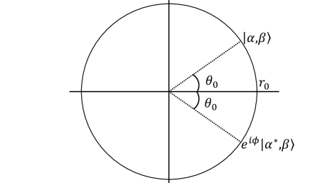
Figure 1: The superposition of two coherent states $|\alpha,\beta\rangle$ and $|\alpha^{*},\beta\rangle$. The radius of the circle is $r_{0}=\sqrt{2\hbar/m_{\mathrm{A}}\omega_{\mathrm{A}}}|\alpha|$ and the angular separation is $2\theta_{0}=2\tan^{-1}({\rm Im}~{}\alpha/{\rm Re}~{}\alpha)$.

Next, we consider two clocks $\mathrm{A}$ and $\mathrm{B}$ and suppose that initially clock $\mathrm{A}$ is in a superposition of two coherent state Schleich et al. (1991):

$$|\psi_{\mathrm{A}}\rangle=\frac{1}{\sqrt{N}}\left(|\alpha,\beta\rangle+e^{i\phi}|\alpha^{\prime},\beta\rangle\right)\,.$$ (35)

Two coherent states are assumed to have the same center of circle, namely the same $\beta$, but have different positions on the circle as shown in Fig. 1 :

$$\alpha = \sqrt{\frac{m_{\mathrm{A}}\omega_{\mathrm{A}}}{2\hbar}}r_{0}e^{i\theta_{0}},$$ (36)

$$\alpha^{\prime} = \sqrt{\frac{m_{\mathrm{A}}\omega_{\mathrm{A}}}{2\hbar}}r_{0}e^{-i\theta_{0}}=\alpha^{*}\,,$$ (37)

which means the angular separation is $2\theta_{0}$ for $0\leq\theta_{0}<\pi$. Two clocks rotate about the center clockwise with the angular velocity $\omega_{\mathrm{A}}$. The normalization factor $N$ is given by

$$N=2+2{\rm Re}\left(e^{-i\phi}\langle\alpha^{\prime},\beta|\alpha,\beta\rangle\right)=2+2{\rm Re}\left(e^{-i\phi}e^{\alpha^{2}-|\alpha|^{2}}\right).$$ (38)

Then, the average of $H_{\mathrm{A}}^{\rm ext}$ is

$$\langle\psi_{\mathrm{A}}|H_{\mathrm{A}}^{\rm ext}|\psi_{\mathrm{A}}\rangle = \hbar\omega_{\mathrm{A}}\left(|\alpha|^{2}+\frac{1}{2}\right)+\frac{2\hbar\omega_{\mathrm{A}}}{N}{\rm Re}\left((\alpha^{2}-|\alpha|^{2})e^{-i\phi}e^{\alpha^{2}-|\alpha|^{2}}\right)$$ (39)

$$= \frac{1}{2}m_{\mathrm{A}}\omega_{\mathrm{A}}r_{0}^{2}+\frac{1}{2}\hbar\omega_{\mathrm{A}}+2\sin\theta_{0}\frac{m_{\mathrm{A}}\omega_{\mathrm{A}}^{2}r_{0}^{2}}{N}{\rm Re}\left(ie^{i(\theta_{0}-\phi)}e^{\alpha^{2}-|\alpha|^{2}}\right).$$

Hence the time dilation between two clocks becomes

$$\langle T_{\mathrm{A}}\rangle=\tau_{\mathrm{B}}\left(1-\frac{\omega_{\mathrm{A}}^{2}r_{0}^{2}}{2c^{2}}-\frac{\hbar\omega_{\mathrm{A}}}{2m_{\mathrm{A}}c^{2}}-2\sin\theta_{0}\frac{\omega_{\mathrm{A}}^{2}r_{0}^{2}}{Nc^{2}}{\rm Re}\left(ie^{i(\theta_{0}-\phi)}e^{\alpha^{2}-|\alpha|^{2}}\right)+\frac{\hbar^{2}}{2m_{\mathrm{B}}^{2}c^{2}\sigma_{\mathrm{B}}^{2}}\right)\,.$$ (40)

The term proportional to $\sin\theta_{0}$ arises from quantum interference due to the superposition and may be regarded as the quantum time dilation.

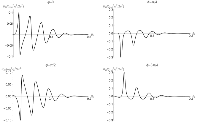
Figure 2: $K_{Q}/(\omega_{\mathrm{A}}^{2}r_{0}^{2}/2c^{2})$ as a function of $\theta_{0}$ for several $\phi$.

To make the effect of quantum time dilation manifest, as in Chiba and Kinoshita (2022) we split the time dilation formula (40) into $K_{C}$ and $K_{Q}$ as $\langle T_{\mathrm{A}}\rangle=\tau_{\mathrm{B}}(1-K_{C}-K_{Q})$. $K_{C}$ is given by the contribution of a statistical mixture of the coherent states of clock $\mathrm{A}$ and clock $\mathrm{B}$, and $K_{Q}$ is the term due to the interference effect

$$K_{C} = \frac{\omega_{\mathrm{A}}^{2}r_{0}^{2}}{2c^{2}}+\frac{\hbar\omega_{\mathrm{A}}}{2m_{\mathrm{A}}c^{2}}-\frac{\hbar^{2}}{2m_{\mathrm{B}}^{2}c^{2}\sigma_{\mathrm{B}}^{2}},$$ (41)

$$K_{Q} = 2\sin\theta_{0}\frac{\omega_{\mathrm{A}}^{2}r_{0}^{2}}{Nc^{2}}{\rm Re}\left(ie^{i(\theta_{0}-\phi)}e^{\alpha^{2}-|\alpha|^{2}}\right)\,.$$ (42)

Positive $K_{Q}$ implies the enhanced time dilation. In Fig. 2, $K_{Q}$ normalized by the classical time dilation factor $\omega_{\mathrm{A}}^{2}r_{0}^{2}/2c^{2}$ is shown. In this example, the charged clock particle is supposed to be $~{}^{40}{\rm Ar}^{13+}$ as in King et al. (2022), and we assumed $q_{\mathrm{A}}=13e$, $m_{\mathrm{A}}=6.6\times 10^{-26}{\rm kg}$, $B=1.0{\rm T}$ and $r_{0}=1.0\times 10^{-7}{\rm m}$, so that the classical time dilation factor becomes $\omega_{\mathrm{A}}^{2}r_{0}^{2}/2c^{2}=5.5\times 10^{-17}$. The quantum effect can either enhance or reduce the time dilation and can be as large as $10\%$ of the classical time dilation. The coherence time of several seconds for maintaining the superposition may be required to observe a quantum time dilation effect, which is an experimental challenge but is well within the measurement capability of state-of-the-art clocks Kovachy et al. (2015).

IV Summary

As an extension of the proper time observable proposed in Smith and Ahmadi (2020) and applied to a weak gravitational field Chiba and Kinoshita (2022), we studied charged quantum clocks interacting with the external electromagnetic fields. We derived a formula of the average proper time read by one clock conditioned on another clock reading a different proper time, Eq. (28), which has the same form as that in classical relativity consisting of kinetic part (velocity squared term) and gravitational part (gravitational redshift term). We found that the time dilation is given by difference of velocity and distance between trajectories of each clock, regardless of whether the clock is in inertial motion or non-inertial motion.

When applied to a charged quantum clock in a uniform magnetic field, we considered the case in which the state of one clock is in a superposition. We found that the effect arising from quantum interference appears in the time dilation which can be as large as $10\%$ of the classical time dilation.

According to the proper time observable, the time dilation is given by the expectation value depending on how one prepared clock particle states as in Eq. (28). In this paper, to analytically estimate deviation from the classical time dilation on the basis of the derived formula, we have considered the simplest clock model and have employed the coherent states which follow trajectories of semi-classical cyclotron motion. However, adopting other states or settings, such as eigenstates of the Hamiltonian and so on, may make it more advantageous to experimentally implement within reach of currently established technologies. For example, Bushev et al. Bushev et al. (2016) have proposed an experiment with a single electron in a Penning trap to probe the time dilation depending on the radial cyclotron state of the electron by using the electronic spin precession as an internal clock.

Optical clocks based on highly charged ions have been considered as a new class of references for highest-accuracy clocks and precision tests of fundamental physics Kozlov et al. (2018). Moreover, such an optical clock based on a highly charged ion was realized recently King et al. (2022). Our study may be relevant in interpreting the measurements of the time dilation of a highly charged optical clock.

Appendix A Quantum Mechanics of a Charged Particle in a Uniform Magnetic Field

Here, we summerize the basic results on quantum mechanics of a charged particle in a uniform magnetic field Landau and Lifshits (1991); Schulman (2005)

A.1 Hamiltonian and Relative Coordinate

Consider a particle with the mass $m$ and the charge $q$ moving in a uniform magnetic field $B$. Take the $z$-axis in the direction of the magnetic field and assume that the particle moves in the $xy$-plane.

The Hamiltonian in the symmetric gauge

$${\bf A}=\frac{1}{2}{\bf B}\times{\bf x}=\frac{B}{2}(-y,x,0)$$ (43)

is given by

$$H=\frac{({\bf p}-q{\bf A})^{2}}{2m}=\frac{1}{2m}\left(p_{x}+\frac{m\omega}{2}y\right)^{2}+\frac{1}{2m}\left(p_{y}-\frac{m\omega}{2}x\right)^{2}\,,$$ (44)

where we have introduced the cyclotron frequency $\omega=qB/m$.

Since the time evolution of position operator is given from the Heisenberg equation by $\dot{x}_{i}=\frac{[x_{i},H]}{i\hbar}=\frac{p_{i}-qA_{i}}{m}$, considering the classical cyclotron motion, we introduce the position operators $X$ and $Y$ corresponding to the center of the circle

$$X=\frac{p_{y}+m\omega x/2}{m\omega},\quad Y=-\frac{p_{x}-m\omega y/2}{m\omega}\,,$$ (45)

and the operators $\xi$ and $\eta$ corresponding to the relative coordinates

$$\xi=x-X=-\frac{p_{y}-m\omega x/2}{m\omega},~{}~{}~{}~{}~{}\eta=y-Y=\frac{p_{x}+m\omega y/2}{m\omega}\,.$$ (46)

Note that both $X$ and $Y$ commute with the Hamiltonian, $[X,H]=0=[Y,H]$, and hence they are conserved, but $X$ and $Y$ do not commute with each other, $[X,Y]=-i\hbar/m\omega$.

A.2 Creation and Annihilation Operators

We introduce the following creation and annihilation operators

$$a = \sqrt{\frac{m\omega}{2\hbar}}\left(\xi+i\eta\right)=\sqrt{\frac{m\omega}{2\hbar}}\left(\left(\frac{x}{2}+i\frac{p_{x}}{m\omega}\right)+i\left(\frac{y}{2}+i\frac{p_{y}}{m\omega}\right)\right),$$ (47)

$$a^{\dagger} = \sqrt{\frac{m\omega}{2\hbar}}\left(\xi-i\eta\right)=\sqrt{\frac{m\omega}{2\hbar}}\left(\left(\frac{x}{2}-i\frac{p_{x}}{m\omega}\right)-i\left(\frac{y}{2}-i\frac{p_{y}}{m\omega}\right)\right),$$ (48)

$$b = \sqrt{\frac{m\omega}{2\hbar}}\left(X-iY\right)=\sqrt{\frac{m\omega}{2\hbar}}\left(\left(\frac{x}{2}+i\frac{p_{x}}{m\omega}\right)-i\left(\frac{y}{2}+i\frac{p_{y}}{m\omega}\right)\right),$$ (49)

$$b^{\dagger} = \sqrt{\frac{m\omega}{2\hbar}}\left(X+iY\right)=\sqrt{\frac{m\omega}{2\hbar}}\left(\left(\frac{x}{2}-i\frac{p_{x}}{m\omega}\right)+i\left(\frac{y}{2}-i\frac{p_{y}}{m\omega}\right)\right),\,$$ (50)

where $a$ and $b$ commute with each other and obey the usual commutation relations

$$[a,a^{\dagger}]=1,~{}~{}~{}~{}~{}[b,b^{\dagger}]=1\,.$$ (51)

Then, the Hamiltonian and the $z$ component of the angular momentum $L_{z}$ are written in terms of $a$ and $b$ in simple form as

$$H = \hbar\omega\left(a^{\dagger}a+\frac{1}{2}\right),$$ (52)

$$L_{z} = xp_{y}-yp_{x}=\hbar(-a^{\dagger}a+b^{\dagger}b)\,.$$ (53)

From Eqs. (47)-(50), the number operator $a^{\dagger}a$ corresponds to the squared distance from the center of the circle and $b^{\dagger}b$ corresponds to the squared distance of the center from the origin of the coordinates.

We also note that the center of the circle and the relative coordinates are written in terms of creation and annihilation operators as

$$X = \frac{1}{2}\sqrt{\frac{2\hbar}{m\omega}}(b+b^{\dagger}),~{}~{}~{}~{}~{}Y=\frac{i}{2}\sqrt{\frac{2\hbar}{m\omega}}(b-b^{\dagger}),$$ (54)

$$\xi = \frac{1}{2}\sqrt{\frac{2\hbar}{m\omega}}(a+a^{\dagger}),~{}~{}~{}~{}~{}\eta=\frac{i}{2}\sqrt{\frac{2\hbar}{m\omega}}(-a+a^{\dagger}).$$ (55)

A.3 Coherent State

As in the case of one-dimensional harmonic oscillator, we introduce the coherent state $|\alpha,\beta\rangle$ such that $a|\alpha,\beta\rangle=\alpha|\alpha,\beta\rangle$ and $b|\alpha,\beta\rangle=\beta|\alpha,\beta\rangle$, which is constructed by applying the operators $e^{\alpha a^{\dagger}}$ and $e^{\beta b^{\dagger}}$ on the ground state $|0\rangle$ as

$$|\alpha,\beta\rangle=e^{-\frac{|\alpha|^{2}+|\beta|^{2}}{2}}e^{\alpha a^{\dagger}}e^{\beta b^{\dagger}}|0\rangle\,.$$ (56)

Then, from Eq. (47) and Eq. (49), the eigenvalues $\alpha$ and $\beta$ corresponding to the relative coordinate $(r_{0}\cos\theta_{0},r_{0}\sin\theta_{0})$ and the center of the circle $(X_{0},Y_{0})$ are given by

$$\alpha = \sqrt{\frac{m\omega}{2\hbar}}r_{0}e^{i\theta_{0}},$$ (57)

$$\beta = \sqrt{\frac{m\omega}{2\hbar}}(X_{0}-iY_{0}).$$ (58)

The wave function of the coherent state is given by

$$\langle{\bf x}|\alpha,\beta\rangle= \sqrt{\frac{m\omega}{2\pi\hbar}}\exp\left\{-\frac{m\omega}{4\hbar}\left[(x-r_{0}\cos\theta_{0}-X_{0})^{2}+(y-r_{0}\sin\theta_{0}-Y_{0})^{2}\right]\right\}$$ (59)

$$\times\exp\left\{i\frac{m\omega}{2\hbar}\left[(r_{0}\sin\theta_{0}-Y_{0})x-(r_{0}\cos\theta_{0}-X_{0})y-r_{0}(X_{0}\sin\theta_{0}-Y_{0}\cos\theta_{0})\right]\right\}.$$

$a(t)$ and $b(t)$ evolve according to the Heisenberg equation as

$$i\hbar\dot{a}(t) = [a(t),H]=\hbar\omega a(t),$$ (60)

$$i\hbar\dot{b}(t) = [b(t),H]=0\,.$$ (61)

Hence, we have $a(t)=e^{-i\omega t}a$ and $b(t)=b$. Then, from Eq. (55), the expectation values of $\xi(t)$ and $\eta(t)$ in the coherent state are given by

$$\langle\xi(t)\rangle = \frac{1}{2}\sqrt{\frac{2\hbar}{m\omega}}\langle\alpha,\beta|(a(t)+a^{\dagger}(t))|\alpha,\beta\rangle=\frac{1}{2}\sqrt{\frac{2\hbar}{m\omega}}(\alpha e^{-i\omega t}+\alpha^{*}e^{i\omega t})=r_{0}\cos(\theta_{0}-\omega t),$$ (62)

$$\langle\eta(t)\rangle = \frac{i}{2}\sqrt{\frac{2\hbar}{m\omega}}\langle\alpha,\beta|(-a(t)+a^{\dagger}(t))|\alpha,\beta\rangle=\frac{1}{2}\sqrt{\frac{2\hbar}{m\omega}}(-\alpha e^{-i\omega t}+\alpha^{*}e^{i\omega t})=r_{0}\sin(\theta_{0}-\omega t)\,.$$ (63)

This corresponds to the position of a charged particle orbiting clockwise about the center with the angular velocity $\omega$. The expectation values of $X(t)$ and $Y(t)$ do not depend on time: $\langle X(t)\rangle=X_{0}$ and $\langle Y(t)\rangle=Y_{0}$.

The expectation value of the Hamiltonian becomes

$$\langle\alpha,\beta|H|\alpha,\beta\rangle=\hbar\omega\left(|\alpha|^{2}+\frac{1}{2}\right)=\frac{1}{2}m\omega^{2}r_{0}^{2}+\frac{1}{2}\hbar\omega.$$ (64)

A.4 Time Dilation in a Rotating Frame

We show that the time dilation Eq. (30) is invariant even if we move to a rotating frame.

Consider a frame $(x^{\prime},y^{\prime})$ which rotates with the angular velocity $\Omega$ about the $z$ axis with respect the inertial frame $(x,y)$. The two coordinates are related by

$$\begin{pmatrix}x^{\prime}\\ y^{\prime}\\ \end{pmatrix}=\begin{pmatrix}\cos\Omega t&\sin\Omega t\\ -\sin\Omega t&\cos\Omega t\\ \end{pmatrix}\begin{pmatrix}x\\ y\\ \end{pmatrix}.$$ (65)

Then, the shift vector appears in the rotating frame

$$-c^{2}dt^{2}+dx^{2}+dy^{2}=-c^{2}dt^{2}+(dx^{\prime}-\Omega y^{\prime}dt)^{2}+(dy^{\prime}+\Omega x^{\prime}dt)^{2},$$ (66)

that is, $\beta^{x^{\prime}}c=-\Omega y^{\prime}$ and $\beta^{y^{\prime}}c=\Omega x^{\prime}$. In the presence of the shift vector, the (external) Hamiltonian becomes $H=\frac{({\bf P}-q{\bf A})^{2}}{2m}-\boldsymbol{\beta}c\cdot({\bf P}-q{\bf A})$, so that the time evolution of the position vector is given by

$$\dot{\bf x}^{\prime}=\frac{[{\bf x}^{\prime},H]}{i\hbar}=\frac{{\bf P}-q{\bf A}}{m}-\boldsymbol{\beta}c\,.$$ (67)

Moreover, from Eq. (65) and Eq. (46), we have

$$\dot{x}^{\prime} = \Omega y^{\prime}+\omega(\eta\cos\Omega t-\xi\sin\Omega t),$$ (68)

$$\dot{y}^{\prime} = -\Omega x^{\prime}-\omega(\xi\cos\Omega t+\eta\sin\Omega t)\,.$$ (69)

Hence

$$\frac{({\bf P}-q{\bf A})^{2}}{m^{2}} = (\dot{x}^{\prime}+\beta^{x^{\prime}}c)^{2}+(\dot{y}^{\prime}+\beta^{y^{\prime}}c)^{2}$$ (70)

$$= \omega^{2}\left(\xi^{2}+\eta^{2}\right)=\dot{x}^{2}+\dot{y}^{2}\,.$$

Therefore, the time dilation formula Eq. (30) holds in a rotating frame. This implies, in particular, that even if we move to a rotating frame with $\Omega=-\omega$ so that a particle is at rest (classically), the time dilation does not change.

References

- Chiba and Kinoshita (2022) T. Chiba and S. Kinoshita, Phys. Rev. D 106, 124035 (2022), arXiv:2209.07638 [gr-qc] .
- Smith and Ahmadi (2020) A. R. H. Smith and M. Ahmadi, Nature Commun. 11, 5360 (2020), arXiv:1904.12390 [quant-ph] .
- Sakurai (1980) J. J. Sakurai, Phys. Rev. D 21, 2993 (1980).
- Kozlov et al. (2018) M. G. Kozlov, M. S. Safronova, J. R. Crespo López-Urrutia, and P. O. Schmidt, Rev. Mod. Phys. 90, 045005 (2018), arXiv:1803.06532 [physics.atom-ph] .
- King et al. (2022) S. A. King et al., Nature 611, 43 (2022), arXiv:2205.13053 [physics.atom-ph] .
- Misner et al. (2017) C. W. Misner, K. S. Thorne, and J. A. Wheeler, Gravitation (Princeton University Press, Princeton, N.J., 2017).
- Page and Wootters (1983) D. N. Page and W. K. Wootters, Phys. Rev. D 27, 2885 (1983).
- Wootters (1984) W. K. Wootters, International Journal of Theoretical Physics 23, 701 (1984).
- Schleich et al. (1991) W. Schleich, M. Pernigo, and F. L. Kien, Phys. Rev. A 44, 2172 (1991).
- Kovachy et al. (2015) T. Kovachy, P. Asenbaum, C. Overstreet, C. A. Donnelly, S. M. Dickerson, A. Sugarbaker, J. M. Hogan, and M. A. Kasevich, Nature 528, 530 (2015).
- Bushev et al. (2016) P. Bushev, J. H. Cole, D. Sholokhov, N. Kukharchyk, and M. Zych, New J. Phys. 18, 093050 (2016), arXiv:1604.06217 [gr-qc] .
- Landau and Lifshits (1991) L. D. Landau and E. M. Lifshits, Quantum Mechanics: Non-Relativistic Theory, Course of Theoretical Physics, Vol. v.3 (Butterworth-Heinemann, Oxford, 1991).
- Schulman (2005) L. S. Schulman, TECHNIQUES AND APPLICATIONS OF PATH INTEGRATION (Dover, 2005).