Partial Identification of Causal Effects Using Proxy Variables
 

Abstract

Proximal causal inference is a recently proposed framework for evaluating the causal effect of a treatment on an outcome variable in the presence of unmeasured confounding (Miao et al., 2018a, ; Tchetgen Tchetgen et al.,, 2020). For nonparametric point identification of causal effects, the framework leverages a pair of so-called treatment and outcome confounding proxy variables, in order to identify a bridge function that matches the dependence of potential outcomes or treatment variables on the hidden factors to corresponding functions of observed proxies. Unique identification of a causal effect via a bridge function crucially requires that proxies are sufficiently relevant for hidden factors, a requirement that has previously been formalized as a completeness condition. However, completeness is well-known not to be empirically testable, and although a bridge function may be well-defined in a given setting, lack of completeness, sometimes manifested by availability of a single type of proxy, may severely limit prospects for identification of a bridge function and thus a causal effect; therefore, potentially restricting the application of the proximal causal framework. In this paper, we propose partial identification methods that do not require completeness and obviate the need for identification of a bridge function. That is, we establish that proxies of unobserved confounders can be leveraged to obtain bounds on the causal effect of the treatment on the outcome even if available information does not suffice to identify either a bridge function or a corresponding causal effect of interest. Our bounds are non-smooth functionals of the underlying distribution. As a consequence, in the context of inference, we initially employ the LogSumExp approximation, which represents a smooth approximation of our bounds. Subsequently, we leverage bootstrap confidence intervals on the approximated bounds. We further establish analogous partial identification results in related settings where identification hinges upon hidden mediators for which proxies are available, however such proxies are not sufficiently rich for point identification of a bridge function or a corresponding causal effect of interest.

Keywords: Causal Effect; Partial Identification; Proximal Causal Inference; Unobserved Confounders; Unobserved Mediators

1 Introduction

Evaluation of the causal effect of a certain treatment variable on an outcome variable of interest from purely observational data is the main focus in many scientific endeavors. One of the most common identification conditions for causal inference from observational data is that of conditional exchangeability. The assumption essentially presumes that the researcher has collected a sufficiently rich set of pre-treatment covariates, such that within the covariate strata, it is as if the treatment were assigned randomly. Unfortunately, this assumption is violated in many real-world settings as it essentially requires that there should not exist any unobserved common causes of the treatment-outcome relation (i.e., no unobserved confounders).

To address the challenge of unobserved confounders, the proximal causal inference framework was recently introduced by Tchetgen Tchetgen and colleagues (Tchetgen Tchetgen et al.,, 2020; Miao et al., 2018a, ). This framework shows that identification of the causal effect of the treatment on outcome in the presence of unobserved confounders still is sometimes feasible provided that one has access to two types of proxy variables of the unobserved confounders, a treatment confounding proxy and an outcome confounding proxy that satisfy certain assumptions. The proximal causal inference framework was recently extended to several other challenging causal inference settings such longitudinal data (Ying et al.,, 2023), mediation analysis (Dukes et al.,, 2023; Ghassami et al., 2021a, ), outcome-dependent sampling (Li et al.,, 2023), network interference settings (Egami and Tchetgen Tchetgen,, 2023), graphical causal models (Shpitser et al.,, 2023), and causal data fusion (Ghassami et al.,, 2022). It has also recently been shown that under an alternative somewhat stronger set of assumptions with regards to proxy relevance, identification is sometimes possible using a single proxy variable (Tchetgen Tchetgen et al.,, 2023).

A key identification condition of proximal causal inference is an assumption that proxies are sufficiently relevant for hidden confounding factors so that there exist a so-called confounding bridge function, defined in terms of proxies, that matches the association between hidden factors and either the potential outcomes or the treatment variable; identification of which is an important step towards identification of causal effects via proxies. However, non-parametric identification of such a bridge function, when it exists, has to date involved a completeness condition which, roughly speaking, requires that variation in proxy variables reflects all sources of variation of unobserved confounders (Tchetgen Tchetgen et al.,, 2020). However, completeness is a strong condition which may significantly limit the researcher’s choice of proxy variables, and hence the feasibility of proximal causal inference in important practical settings where the assumption cannot reasonably be assumed to hold. For instance, in many settings, only one of the two required types of proxies may be available rendering point identification infeasible, even if the proxies are highly relevant. More broadly, point identification of causal effects using existing proximal causal inference methods crucially relies on identification of a confounding bridge function, and remains possible even if the latter is only set-identified (Zhang et al.,, 2023; Bennett et al.,, 2023). Notably, failure to identify such a confounding bridge function is generally inevitable without a completeness condition; in which case partial identification of causal effects may be the most one can hope for.

In this paper, we propose partial identification methods for causal parameters using proxy variables in settings where completeness assumptions do not necessarily hold. Therefore, our methods obviate the need for identification of bridge functions which are solutions to integral equations that involve unobserved variables. We provide methods in single proxy settings and demonstrate that certain conditional independence requirements in that setting can be relaxed in case that the researcher has access to a second proxy variable. For the causal parameter of interest, we initially focus on the average treatment effect (ATE) and the effect of the treatment on the treated (ETT) in Sections 2 and 3. Then we extend our results in Section 4 to partial identification in related settings where identification hinges upon hidden mediators for which proxies are available, however such proxies fail to satisfy a completeness condition which would in principle guarantee point identification of the causal effect of interest; such settings include causal mediation with a mis-measured mediator and hidden front-door models. Our bounds are non-smooth functionals of the observed data distribution. As a consequence, in the context of inference, in Section 5, we initially employ the LogSumExp approximation, which represents a smooth approximation of our bounds. Subsequently, we leverage bootstrap confidence intervals on the approximated bounds.

2 Partial Identification Using a Single Proxy

Consider a setting with a binary treatment variable $A\in\{0,1\}$, an outcome variable $Y\in\mathcal{Y}\subseteq[0,+\infty)$, and observed and unobserved confounders denoted by $X$ and $U$, respectively. We are interested in identifying the effect of the treatment on the treated (ETT), which is defined as

$$\theta_{ETT}=\mathbb{E}[Y^{(A=1)}\mid A=1]-\mathbb{E}[Y^{(A=0)}\mid A=1],$$

as well as the average treatment effect (ATE) of $A$ on $Y$ defined as

$$\theta_{ATE}=\mathbb{E}[Y^{(A=1)}]-\mathbb{E}[Y^{(A=0)}],$$

where $Y^{(A=a)}$ is the potential outcome variable representing the outcome had the treatment (possibly contrary to fact) been set to value $a$. Due to the presence of the latent confounder $U$ in the system, without any extra assumptions, ETT and ATE are not point identified. Therefore, we focus on partial identification of conditional potential outcome mean parameters, $\mathbb{E}[Y^{(A=a)}\mid A=1-a]$, and marginal potential outcome mean, $\mathbb{E}[Y^{(A=a)}]$, for $a\in\{0,1\}$.

2.1 Partial Identification Using an Outcome Confounding Proxy

Let $W$ be a proxy of the unobserved confounder, which can be say an error-prone measurement of $U$, or a so-called negative control outcome (Lipsitch et al.,, 2010; Shi et al., 2020b, ). We show that under some requirements on $W$, the proxy can be leveraged to obtain bounds on the parameters $\mathbb{E}[Y^{(A=a)}\mid A=1-a]$ and $\mathbb{E}[Y^{(A=a)}]$. Our requirements on $W$ are as follows.

Figure 1: Example of a graphical model satisfying Assumption 1.

Assumption 1.

The proxy variable is independent of the treatment variable conditional on the confounders, i.e., $W\perp\mkern-9.5mu\perp A\mid\{X,U\}$.

We refer to a proxy variable $W$ satisfying Assumption 1 as an outcome confounding proxy variable.

Assumption 2.

There exists a non-negative bridge function $h$ such that almost surely

$$\mathbb{E}[Y\mid A,X,U]=\mathbb{E}[h(W,A,X)\mid A,X,U].$$

Assumption 1 indicates how the proxy variable is related to other variables in the system. Mainly it states that as a proxy for $U$, $W$ would become irrelevant about the treatment process, and therefore not needed for confounding control had $U$ been observed. This is clearly a non-testable assumption which must therefore be grounded in prior expert knowledge. Figure 1 demonstrates an example of a graphical model that satisfies Assumption 1. Assumption 2 requires the existence of a so-called outcome confounding bridge function which depends on $W$ and whose conditional expectation matches the potential outcome mean, given $U$. The assumption formalizes the idea that $W$ is sufficiently rich so that there exists at least one transformation of the latter which can on average recover the potential outcome as a function of unmeasured confounders. The assumption was initially introduced by Miao et al., 2018b who give sufficient completeness and other regularity conditions for point identification of such a bridge function. Note that we deliberately avoid such assumptions, and therefore cannot generally identify or estimate such a bridge function from observational data, because the integral equation defined in Assumption 2 involves the unobserved confounder $U$. Besides Assumptions 1 and 2, we also have the following requirements on the variables.

Assumption 3.

• For all values $a$, we have $Y^{(A=a)}\perp\mkern-9.5mu\perp A\mid\{X,U\}$.

• For all values $a$, we have $p(A=a\mid X,U)>0$.

• If $A=a$, we have $Y^{(A=a)}=Y$.

Part 1 of Assumption 3 requires independence of the potential outcome variable and the treatment variable conditioned on both observed and unobserved confounders. Note that this is a much milder assumption compared to the standard conditional exhchangeability assumption as we also condition on the unobserved confounders. Parts 2 and 3 of Assumption 3 are the positivity and consistency assumptions, which are standard assumptions in the field of causal identification.

We have the following partial identification result for the conditional potential outcome mean.

Theorem 1.

Under Assumptions 1-3, the parameter $\mathbb{E}[Y^{(A=a)}\mid A=1-a]$ can be bounded as follows.

$$\max\Big{\{}\inf\mathcal{Y}~{},~{}\mathbb{E}\Big{[}\min_{w}\frac{p(w\mid A=1-a,X)}{p(w\mid A=a,X)}\mathbb{E}[Y\mid A=a,X]\Big{|}A=1-a\Big{]}\Big{\}}$$

$$\leq\mathbb{E}[Y^{(A=a)}\mid A=1-a]\leq$$

$$\min\Big{\{}\sup\mathcal{Y}~{},~{}\mathbb{E}\Big{[}\max_{w}\frac{p(w\mid A=1-a,X)}{p(w\mid A=a,X)}\mathbb{E}[Y\mid A=a,X]\Big{|}A=1-a\Big{]}\Big{\}}.$$

We have the following corollary for partial identification of marginal potential outcome mean.

Corollary 1.

Under Assumptions 1-3, the parameter $\mathbb{E}[Y^{(A=a)}]$ can be bounded as follows.

$$\max\Big{\{}\inf\mathcal{Y}\times p(A=1-a)+\mathbb{E}[Y\mid A=a]p(A=a),\mathbb{E}\Big{[}\frac{I(A=a)}{\max_{w}p(a\mid w,X)}Y\Big{]}\Big{\}}$$

$$\leq\mathbb{E}[Y^{(A=a)}]\leq$$

$$\min\Big{\{}\sup\mathcal{Y}\times p(A=1-a)+\mathbb{E}[Y\mid A=a]p(A=a),\mathbb{E}\Big{[}\frac{I(A=a)}{\min_{w}p(a\mid w,X)}Y\Big{]}\Big{\}},$$

where $I(\cdot)$ is the indicator function.

Several remarks are in order regarding the proposed bounds.

Remark 1.

Note that if there are no unobserved confounders in the system, $A$ and $W$ are independent conditional on $X$ and hence, the upper and lower bound in Theorem 1 and Corollary 1 will match. Especially, those in Corollary 1 will be equal to the standard inverse probability weighting (IPW) identification formula in the conditional exchangeability framework. Furthermore, the bounds can be written as

$$\max\Big{\{}\inf\mathcal{Y}\times p(A=1-a)+\mathbb{E}[Y\mid A=a]p(A=a),\mathbb{E}\Big{[}\frac{p(a\mid X)}{\max_{w}p(a\mid w,X)}\mathbb{E}[Y\mid A=a,X]\Big{]}\Big{\}}$$

$$\leq\mathbb{E}[Y^{(A=a)}]\leq$$

$$\min\Big{\{}\sup\mathcal{Y}\times p(A=1-a)+\mathbb{E}[Y\mid A=a]p(A=a),\mathbb{E}\Big{[}\frac{p(a\mid X)}{\min_{w}p(a\mid w,X)}\mathbb{E}[Y\mid A=a,X]\Big{]}\Big{\}},$$

which demonstrates the connection to the g-formula in the conditional exchangeability framework (Hernán and Robins,, 2020). Formally, when $A$ and $W$ are independent conditioned on $X$, we have $\mathbb{E}\Big{[}\frac{p(a\mid X)}{\max_{w}p(a\mid w,X)}\mathbb{E}[Y\mid A=a,X]\Big{]}=\mathbb{E}\big{[}\mathbb{E}[Y\mid A=a,X]\big{]}$, which is the $g$-formula, and for the lower bound, we have

$$\inf\mathcal{Y}\times p(A=1-a)+\mathbb{E}[Y\mid A=a]p(A=a)$$

$$=\sum_{x}\mathbb{E}[\inf\mathcal{Y}\mid A=a,X=x]\times p(A=1-a,X=x)+\sum_{x}\mathbb{E}[Y\mid A=a,X=x]p(A=a,X=x)$$

$$\leq\sum_{x}\mathbb{E}[Y\mid A=a,X=x]\times p(A=1-a,X=x)+\sum_{x}\mathbb{E}[Y\mid A=a,X=x]p(A=a,X=x)$$

$$=\mathbb{E}\big{[}\mathbb{E}[Y\mid A=a,X]\big{]}.$$

That is, the lower bound will be the g-formula. Similar argument holds for the upper bound.

Remark 2.

In the setting considered in this work we assumed $\mathcal{Y}\subseteq[0,+\infty)$. This assumption is merely for the sake of clarity of the presentation and can be relaxed to assuming the outcome is bounded from below. If $\inf\mathcal{Y}<0$, without loss of generality, for the bridge function $h$, we can have $\inf\mathcal{Y}\leq h^{\prime}_{m}\leq h(w,a,x)$, for all $w,a,x$. Let $h_{m}=|\min\{h^{\prime}_{m},0\}|$. Then the bounding step of the proof of Theorem 1 should be changed to

$$\sum_{x}\min_{w}\frac{p(w\mid A=1-a,x)}{p(w\mid A=a,x)}\sum_{w}h(w,a,x)p(w\mid A=a,x)p(x\mid A=1-a)$$

$$\qquad+h_{m}\Big{\{}\mathbb{E}\Big{[}\min_{w}\frac{p(w\mid A=1-a,X)}{p(w\mid A=a,X)}\Big{|}A=1-a\Big{]}-1\Big{\}}$$

$$\leq\mathbb{E}[Y^{(A=a)}\mid A=1-a]\leq$$

$$\sum_{x}\max_{w}\frac{p(w\mid A=1-a,x)}{p(w\mid A=a,x)}\sum_{w}h(w,a,x)p(w\mid A=a,x)p(x\mid A=1-a)$$

$$\qquad+h_{m}\Big{\{}\mathbb{E}\Big{[}\max_{w}\frac{p(w\mid A=1-a,X)}{p(w\mid A=a,X)}\Big{|}A=1-a\Big{]}-1\Big{\}}.$$

Remark 3.

If we are only interested in partially identifying ETT, then we only need bounds for the parameter $\mathbb{E}[Y^{(A=0)}\mid A=1]$. In this case, Assumption 2 can be weakened to requiring the existence of a bridge function $h$ such that almost surely

$$\mathbb{E}[Y\mid A=0,X,U]=\mathbb{E}[h(W,X)\mid X,U].$$

Remark 4.

In case that we have access to several proxy variables $\{W_{1},...,W_{K}\}$ which satisfy Assumptions 1 and 2, a method for improving the bounds would be to construct bounds based on each proxy variable and then choose the upper bound to be the minimum of the upper bounds and choose the lower bound to be the maximum of the lower bounds.

2.2 Partial Identification Using a Treatment Confounding Proxy

The proxy variable $W$ is potentially directly associated with the outcome variable but is required to be conditionally independent from the treatment variable. In this subsection, we establish an alternative partial identification method based on a proxy variable $Z$ of the unobserved confounder, which can be directly associated with the treatment variable, but is required to be conditionally independent of the outcome variable. Formally, we have the following requirements on the proxy variable $Z$.

Assumption 4.

The proxy variable $Z$ is independent of the outcome variable conditional on the confounders and the treatment variable, i.e., $Z\perp\mkern-9.5mu\perp Y\mid A,X,U$.

We refer to a proxy variable satisfying Assumption 4 as a treatment confounding proxy variable. Figure 2 demonstrates an example of a graphical model that satisfies Assumption 4.

Figure 2: Example of a graphical model satisfying Assumption 4.

Assumption 5.

There exists a non-negative bridge function $q$ such that almost surely

$$\mathbb{E}[q(Z,A,X)\mid A,X,U]=\frac{p(U\mid 1-A,X)}{p(U\mid A,X)}.$$

Existence of similar treatment confounding bridge function was first discussed by Deaner, (2018) and Cui et al., (2023) who also imposed additional conditions, including completeness, such that the treatment bridge function and causal effects are both uniquely nonparametrically identified. As in the previous section, we do not make such additional assumptions.

We have the following partial identification result for the conditional potential outcome mean.

Theorem 2.

Under Assumptions 3-5, the parameter $\mathbb{E}[Y^{(A=a)}\mid A=1-a]$ can be bounded as follows.

$$\mathbb{E}\big{[}\min_{z}\mathbb{E}[Y\mid z,X,A=a]\big{|}A=1-a\big{]}$$

$$\leq\mathbb{E}\big{[}Y^{(A=a)}\mid A=1-a]\leq$$

$$\mathbb{E}\big{[}\max_{z}\mathbb{E}[Y\mid z,X,A=a]\big{|}A=1-a\big{]}.$$

We have the following corollary for partial identification of marginal potential outcome mean.

Corollary 2.

Under Assumptions 3-5, the parameter $\mathbb{E}[Y^{(A=a)}]$ can be bounded as follows.

$$\mathbb{E}\big{[}\min_{z}\mathbb{E}[Y\mid z,X,A=a]\big{|}A=1-a\big{]}p(A=1-a)+\mathbb{E}[Y\mid A=a]p(A=a)$$

$$\leq\mathbb{E}[Y^{(A=a)}]\leq$$

$$\mathbb{E}\big{[}\max_{z}\mathbb{E}[Y\mid z,X,A=a]\big{|}A=1-a\big{]}p(A=1-a)+\mathbb{E}[Y\mid A=a]p(A=a).$$

Several remarks are in order regarding the proposed bounds.

Remark 5.

Note that in Theorem 2, the lower bound will not be smaller than $\inf\mathcal{Y}$ and hence unlike Theorem 1, we do not need to consider $\inf\mathcal{Y}$. Similarly, the upper bound will not be larger than $\sup\mathcal{Y}$.

Remark 6.

Note that if there are no unobserved confounders in the system, $Y$ and $Z$ are independent conditional on $A$ and $X$, providing a clear connection of the bounds in Theorem 2 and Corollary 2 to the IPW and g-formula identification methods in the conditional exchangeability framework given $X$ only.

Remark 7.

If we are only interested in partially identifying ETT, then we only need bounds for the parameter $\mathbb{E}[Y^{(A=0)}\mid A=1]$. In this case, Assumption 5 can be weakened to requiring the existence of a bridge function $q$ such that almost surely

$$\mathbb{E}[q(Z,X)\mid A=0,X,U]=\frac{p(U\mid A=1,X)}{p(U\mid A=0,X)}.$$

Remark 8.

Similar to the case of outcome confounding proxies, in case that we have access to several proxy variables $\{Z_{1},...,Z_{K}\}$ which satisfy Assumptions 4 and 5, a method for improving the bounds would be to construct bounds based on each proxy variable and then choose the upper bound to be the minimum of the upper bounds and choose the lower bound to be the maximum of the lower bounds.

3 Partial Identification Using Two Independent Invalid Proxies

In this section, we show that having access to two conditionally independent but invalid proxy variables of the unobserved confounder, one can relax the requirements of conditional independence of proxy variables from the treatment and the outcome variables while still providing valid bounds for the treatment effect. The proxy variables in our setting do not necessarily satisfy the strong exclusion restrictions of the original proximal causal inference. Therefore, the point identification approach in the original framework cannot be used here. We require the existence of two proxy variables $W$ and $Z$ that satisfy the following.

Figure 3: Example of a graphical model consistent with the two proxy setting.

Assumption 6.

• The proxy variables are independent conditional on the treatment variable and all confounders, i.e., $W\perp\mkern-9.5mu\perp Z\mid\{A,X,U\}$.

• The invalid proxy variables satisfy Assumptions 2 and 5.

Figure 3 demonstrates an example of a graphical model consistent with our two-proxy setting. Note that neither proxy variable $W$ technically needs to be an outcome confounding proxy variable (defined in Assumption 1) nor proxy variable $Z$ needs to be a treatment confounding proxy variable (defined in Assumption 4). Specifically, there can exist a direct causal link between $A$ and $W$ and one between $Z$ and $Y$ (shown in the figure by the red edges).

We have the following partial identification result for the conditional potential outcome mean.

Theorem 3.

Under Assumptions 3 and 6, the parameter $\mathbb{E}[Y^{(A=a)}\mid A=1-a]$ can be bounded as follows.

$$\max\Big{\{}\inf\mathcal{Y}~{},~{}\mathbb{E}\Big{[}\min_{w,z}\frac{p(w,z\mid a,X)}{p(w\mid a,X)p(z\mid a,X)}\mathbb{E}[Y\mid A=a,X]\Big{|}A=1-a\Big{]}\Big{\}}$$

$$\leq\mathbb{E}[Y^{(A=a)}\mid A=1-a]\leq$$

$$\min\Big{\{}\sup\mathcal{Y}~{},~{}\mathbb{E}\Big{[}\max_{w,z}\frac{p(w,z\mid a,X)}{p(w\mid a,X)p(z\mid a,X)}\mathbb{E}[Y\mid A=a,X]\Big{|}A=1-a\Big{]}\Big{\}}.$$

Note that in the absence of the unobserved confounder $U$, $\min_{w,z}p(w,z\mid a,x)=\max_{w,z}p(w,z\mid a,x)=p(w\mid a,x)p(z\mid a,x)$. Hence, again the upper and lower bounds match and will be equal to the g-formula and IPW formula in the conditional exchangeability framework given $X$.

4 Partial Identification in the Presence of Unobserved Mediators

In this Section we show that our partial identification ideas can also be used for dealing with unobserved mediators in the system. The results in this section are the counterparts of the results of Ghassami et al., 2021a where the authors obtained point identification results under completeness assumptions. We focus on two settings with hidden mediators: Mediation analysis and front-door model. We only show the extension of the method presented in Subsection 2.1 and do not repeat extensions for the methods of Sections 2.2 and 3, although they are easily deduced from our exposition.

Let $M$ be the mediator variable in the system which is unobserved. We denote the potential outcome variable of $Y$, had the treatment and mediator variables been set to value $A=a$ and $M=m$ (possibly contrary to the fact) by $Y^{(a,m)}$. Similarly, we define $M^{(a)}$ as the potential outcome variable of $M$ had the treatment variables been set to value $A=a$. Based on variables $Y^{(a,m)}$ and $M^{(a)}$, we define $Y^{(a)}=Y^{(a,M^{(a)})}$, and $Y^{(m)}=Y^{(A,m)}$. We posit the following standard assumptions on the model.

Assumption 7.

• For all $m$, $a$, and $x$, we have $p(m\mid a,x)>0$, and $p(a\mid x)>0$.

• $M^{(a)}=M$ if $A=a$. $Y^{(a,m)}=Y$ if $A=a$ and $M=m$.

4.1 Partial Identification of NIE and NDE

We first focus on mediation analysis. The goal is to identify the direct and indirect parts of the ATE, i.e., the part mediated through the mediator variable and the rest of the ATE. This can be done noting the following presentation of the ATE.

$$\mathbb{E}[Y^{(1)}-Y^{(0)}] =\mathbb{E}[Y^{(1,M^{(1)})}-Y^{(0,M^{(0)})}]$$

$$=\mathbb{E}[Y^{(1,M^{(1)})}-Y^{(1,M^{(0)})}]+\mathbb{E}[Y^{(1,M^{(0)})}-Y^{(0,M^{(0)})}].$$

The first and the second terms in the last expression are called the total indirect effect and the pure direct effect, respectively by Robins and Greenland, (1992), and are called the natural indirect effect (NIE) and the natural direct effect (NDE) of the treatment on the outcome, respectively by Pearl, (2001). We follow the latter terminology. NIE can be interpreted as the potential outcome mean if the treatment is fixed at $A=1$ from the point of view of the outcome variable but changes from $A=1$ to $A=0$ from the point of view of the mediator variable. Similarly, NDE can be interpreted as the potential outcome mean if the treatment is changed via intervention from $A=1$ to $A=0$ from the point of view of the outcome variable but is fixed at $A=0$ from the point of view of the mediator variable. We investigate identification of NIE and NDE in case the underlying mediator is hidden, however under the assumption that the model does not contain any hidden confounder. This can be formalized as follows (Imai et al.,, 2010).

Assumption 8.

For any two values of the treatment $a$ and $a^{\prime}$, and value of the mediator $m$, we have $(i)$ $Y^{(a,m)}\perp\mkern-9.5mu\perp A\mid X$, $(ii)$ $M^{(a)}\perp\mkern-9.5mu\perp A\mid X$, and $(iii)$ $Y^{(a,m)}\perp\mkern-9.5mu\perp M^{(a^{\prime})}\mid X$.

Due to Assumption 8, the parameters $\mathbb{E}[Y^{(1,M^{(1)})}]$ and $\mathbb{E}[Y^{(0,M^{(0)})}]$ are point identified. Hence, we focus on the parameter $\mathbb{E}[Y^{(1,M^{(0)})}]$. The identification formula for the this functional, known as the mediation formula in the literature (Pearl,, 2001; Imai et al.,, 2010) requires observing the mediator variable. Here we show that in the setting with unobserved mediator, this parameter can be partially identified provided that we have access to a proxy variable $W$ of the hidden mediator. We have the following requirements on the proxy variable.

Figure 4: Example of a graphical model that satisfies Assumptions 8 and 9.

Assumption 9.

The proxy variable is independent of the treatment variable conditional on the mediator variable and the observed confounder variable, i.e., $W\perp\mkern-9.5mu\perp A\mid\{X,M\}$.

Figure 4 demonstrates an example of a graphical model that satisfies Assumptions 8 and 9.

Assumption 10.

There exists a non-negative bridge function $h$ such that almost surely

$$\mathbb{E}[Y\mid A=1,X,M]=\mathbb{E}[h(W,X)\mid X,M].$$

We have the following partial identification result for the parameter $\mathbb{E}[Y^{(1,M^{(0)})}]$.

Theorem 4.

Under Assumptions 7-10, the parameter $\mathbb{E}[Y^{(1,M^{(0)})}]$ can be bounded as follows.

$$\max\Big{\{}\inf\mathcal{Y}~{},~{}\mathbb{E}\Big{[}\min_{w}\frac{p(w\mid A=0,X)}{p(w\mid A=1,X)}\mathbb{E}[Y\mid A=1,X]\Big{]}\Big{\}}$$

$$\leq\mathbb{E}[Y^{(1,M^{(0)})}]\leq$$

$$\min\Big{\{}\sup\mathcal{Y}~{},~{}\mathbb{E}\Big{[}\max_{w}\frac{p(w\mid A=0,X)}{p(w\mid A=1,X)}\mathbb{E}[Y\mid A=1,X]\Big{]}\Big{\}}.$$

4.2 Partial Identification of ATE in the Front-Door Model

Front-door model is one of the earliest models introduced in the literature of causal inference in which the causal effect of a treatment variable on an outcome variable is identified despite allowing for the treatment-outcome relation to have an unobserved confounder and without any assumptions on the form of the structural equations of the variables (Pearl,, 2009). The main assumption of this framework is that the causal effect of the treatment variable on the outcome variable is fully relayed by a mediator variable, and neither the treatment-mediator relation nor the mediator-outcome relation have an unobserved confounder. This assumption is formally stated as follows.

Assumption 11.

• For any value $a$ of the treatment and value $m$ of the mediator, we have $(i)$ $M^{(a)}\perp\mkern-9.5mu\perp A\mid X$, and $(ii)$ $Y^{(m)}\perp\mkern-9.5mu\perp M\mid A,X$.

• For any value $a$ of the treatment and value $m$ of the mediator, we have $Y^{(a,m)}=Y^{(m)}$.

The identification formula for the front-door model requires observations of the mediator variable. Here we show that in the setting with unobserved mediator, the causal effect of the treatment variable on the outcome variable can be partially identified provided that we have access to a proxy variable $W$ of the hidden mediator which satisfies Assumptions 9 and the following assumption pertaining to the existence of a bridge function. Figure 5 demonstrates an example of a graphical model that satisfies Assumptions 9 and 11.

Figure 5: Example of a graphical model that satisfies Assumptions 9 and 11.

Assumption 12.

There exists a non-negative bridge function $h$ such that almost surely

$$\mathbb{E}[Y\mid A,X,M]=\mathbb{E}[h(W,A,X)\mid A,X,M].$$

We have the following partial identification result for the potential outcome mean.

Theorem 5.

Under Assumptions 7, 9, 11, and 12, the parameter $\mathbb{E}[Y^{(A=a)}]$ can be bounded as follows.

$$\mathbb{E}[I(A=a)Y]+\max\Big{\{}\inf\mathcal{Y}\times p(A=1-a),\mathbb{E}\Big{[}I(A=1-a)\min_{w}\frac{p(w\mid a,X)}{p(w\mid 1-a,X)}Y\Big{]}\Big{\}}$$

$$\leq\mathbb{E}[Y^{(A=a)}]\leq$$

$$\mathbb{E}[I(A=a)Y]+\min\Big{\{}\sup\mathcal{Y}\times p(A=1-a),\mathbb{E}\Big{[}I(A=1-a)\max_{w}\frac{p(w\mid a,X)}{p(w\mid 1-a,X)}Y\Big{]}\Big{\}}.$$

5 Estimation and Inference

So far, we presented non-parametric partial identification formulae for causal parameters in the presence of unobserved confounders or mediators. In this section, we focus on the estimation aspect of the bounds. We restrict our analysis to the scenario where all variables involved are categorical in nature. However, it is worth noting that our findings possess the potential for extension to situations where the observed confounders $X$ and the outcome variable $Y$ are continuous. Nonetheless, such an extension necessitates careful consideration of selecting suitable statistical models to mitigate bias or ensure satisfactory convergence rates. For the results in this section, we only focus on the bounds for conditional potential outcome mean $\mathbb{E}[Y^{(A=a)}\mid A=1-a]$ in Section 2; the proposed approach can be applied to the bounds in Sections 3 and 4.

For the case of categorical variables, it is relatively straightforward to estimate the bounds for the conditional potential outcome mean by employing the formulae outlined in Theorems 1 and 2. However, it is important to acknowledge that these bounds represent non-smooth functionals of the underlying distribution. Consequently, a naive implementation of the bootstrap may result in confidence intervals that are invalid and unreliable. To circumvent this issue, we propose the use of smooth approximations of the aforementioned functionals, described as follows.

Consider a finite set of real numbers $\{x_{1},...,x_{n}\}$. Define the LogSumExp (LSE) function, $LSE(\cdot;\alpha)$ as

$$LSE(\{x_{1},...,x_{n}\};\alpha)=\frac{1}{\alpha}\log\Big{(}\sum_{i=1}^{n}\exp(\alpha x_{i})\Big{)}.$$

It can be shown that $LSE(\{x_{1},...,x_{n}\};\alpha)$ can be used to approximate the maximum and minimum of $\{x_{1},...,x_{n}\}$: for any choice of $\alpha>0$, we have

$$\max\{x_{1},...,x_{n}\}<LSE(\{x_{1},...,x_{n}\};\alpha)\leq\max\{x_{1},...,x_{n}\}+\frac{\log(n)}{\alpha}.$$

Similarly, for any choice of $\alpha<0$, we have

$$\min\{x_{1},...,x_{n}\}+\frac{\log(n)}{\alpha}\leq LSE(\{x_{1},...,x_{n}\};\alpha)<\min\{x_{1},...,x_{n}\}.$$

Therefore, $LSE(\{x_{1},...,x_{n}\};\alpha)$ approximates the maximum and the minimum of $\{x_{1},...,x_{n}\}$ as $\alpha$ tends to $\infty$ and $-\infty$, respectively. Applications of LSE approximation approach has appeared in the fields of optimization (Boyd and Vandenberghe,, 2004), machine learning (Murphy,, 2012; Goodfellow et al.,, 2016; Calafiore et al.,, 2019, 2020), and statistics (Wainwright,, 2019; Chernozhukov et al.,, 2012; Tchetgen Tchetgen and Wirth,, 2017; Levis et al.,, 2023). Notably, Tchetgen Tchetgen and Wirth, (2017) and Levis et al., (2023) employed this approximation technique to facilitate statistical inference pertaining to bounds within the instrumental variables model for missing data and causal effects, respectively.

Applying the LSE function to the bounds in Theorems 1 and 2, we have the following result.

Corollary 3.

• Let $r_{W}(X;\alpha)=LSE(\{\frac{p(w\mid A=1-a,X)}{p(w\mid A=a,X)}\}_{w\in\mathcal{W}};\alpha)$, $\psi_{LW}(\alpha)=LSE(\{\inf\mathcal{Y},\mathbb{E}[r_{W}(X;-\alpha)\mathbb{E}[Y\mid A=a,X]\mid A=1-a]\};\alpha)-\log(2)/\alpha$, and $\psi_{UW}(\alpha)=LSE(\{\sup\mathcal{Y},\mathbb{E}[r_{W}(X;\alpha)\mathbb{E}[Y\mid A=a,X]\mid A=1-a]\};-\alpha)+\log(2)/\alpha$. Under the assumptions of Theorem 1, for any $\alpha>0$, we have

  $$\psi_{LW}(\alpha)\leq\mathbb{E}[Y^{(A=a)}\mid A=1-a]\leq\psi_{UW}(\alpha).$$

• Let $r_{Z}(X;\alpha)=LSE(\{\mathbb{E}[Y\mid z,X,A=a]\}_{z\in\mathcal{Z}};\alpha)$, $\psi_{LZ}(\alpha)=\mathbb{E}[r_{Z}(X;-\alpha)\mid A=1-a]$, and $\psi_{UZ}(\alpha)=\mathbb{E}[r_{Z}(X;\alpha)\mid A=1-a]$. Under the assumptions of Theorem 2, for any $\alpha>0$, we have

  $$\psi_{LZ}(\alpha)\leq\mathbb{E}\big{[}Y^{(A=a)}\mid A=1-a]\leq\psi_{UZ}(\alpha).$$

Equipped with the bounds in Corollary 3, which are smooth functionals of the underlying distribution, the standard bootstrap technique can be used to acquire valid confidence intervals. Formally, for $\psi(\alpha)\in\{\psi_{LW}(\alpha),\psi_{UW}(\alpha),\psi_{LZ}(\alpha),\psi_{UZ}(\alpha)\}$, let $\hat{\psi}_{n}(\alpha)$ denote our estimator based on $n$ samples, $\hat{\psi}^{*}_{n,1}(\alpha),...,\hat{\psi}^{*}_{n,B}(\alpha)$ denote $B$ bootstrap replications of $\hat{\psi}_{n}(\alpha)$, and $\psi^{*}_{\beta}(\alpha)$ denote the $\beta$ sample quantile of the bootstrap replications. Using Part (a) of Corollary 3, we have the following 95% confidence interval for the conditional potential outcome mean

$$C_{{W}_{n}}(\alpha)=\Big{(}2\hat{\psi}_{{LW}_{n}}(\alpha)-\hat{\psi}^{*}_{{LW}_{1-0.05/2}}(\alpha),2\hat{\psi}_{{UW}_{n}}(\alpha)-\hat{\psi}^{*}_{{UW}_{0.05/2}}(\alpha)\Big{)}.$$

Using Part (b) of Corollary 3, we have the following 95% confidence interval for the conditional potential outcome mean

$$C_{{Z}_{n}}(\alpha)=\Big{(}2\hat{\psi}_{{LZ}_{n}}(\alpha)-\hat{\psi}^{*}_{{LZ}_{1-0.05/2}}(\alpha),2\hat{\psi}_{{UZ}_{n}}(\alpha)-\hat{\psi}^{*}_{{UZ}_{0.05/2}}(\alpha)\Big{)}.$$

6 Simulation Studies

In this section, we provide simulation results to demonstrate the performance of our proposed estimators. We designed the data generating process for variables $(U,X,W,Z,A,Y)$ as follows.

• $p(U,X)$: We chose $|\mathcal{U}|\times|\mathcal{X}|$ parameters for the joint distribution $p(U,X)$ uniformly from $Unif[0.1,1]$, and normalized them to sum up to one.

• $p(W\mid U,X)$: For any $w,u,x$,

  $$p(W=w\mid U=u,X=x)=\frac{\exp(\beta_{w,0}+\beta_{w,U}u+\beta_{w,X}x)}{\sum_{w\in\mathcal{W}}\exp(\beta_{w,0}+\beta_{w,U}u+\beta_{w,X}x)}.$$

• $p(Z\mid U,X)$: For any $z,u,x$,

  $$p(Z=z\mid U=u,X=x)=\frac{\exp(\beta_{z,0}+\beta_{z,U}u+\beta_{z,X}x)}{\sum_{z\in\mathcal{Z}}\exp(\beta_{z,0}+\beta_{z,U}u+\beta_{z,X}x)}.$$

• $p(A\mid U,X,Z)$: For any $a,u,x,z$,

  $$p(A=a\mid U=u,X=x,Z=z)=\frac{\exp(\beta_{a,0}+\beta_{a,U}u+\beta_{a,X}x+\beta_{a,Z}z)}{\sum_{a\in\mathcal{A}}\exp(\beta_{a,0}+\beta_{a,U}u+\beta_{a,X}x+\beta_{a,Z}z)}.$$

• $p(Y\mid U,X,W,A)$: For any $y,u,x,w,a$,

  $$p(Y=y\mid U=u,X=x,W=w,A=a)=\frac{\exp(\beta_{y,0}+\beta_{y,U}u+\beta_{y,X}x+\beta_{y,W}w+\beta_{y,A}a)}{\sum_{y\in\mathcal{Y}}\exp(\beta_{y,0}+\beta_{y,U}u+\beta_{y,X}x+\beta_{y,Z}z+\beta_{y,A}a)}.$$

In all the conditional distributions above, coefficients $\beta_{\cdot,\cdot}$ are chosen according to uniform distribution $Unif[-0.5,0.5]$. We require the coefficients connecting $U$ to $W$ and $Z$ to be non-zero to ensure that $W$ and $Z$ are relevant to the latent confounder $U$.

6.1 Simulation Study 1

We first considered the case that $|\mathcal{U}|=|\mathcal{W}|=|\mathcal{Z}|$. In this case, based on the results of Miao et al., 2018a and Shi et al., 2020a , the bridge functions $h$ and $q$ exist. Consequently, in conjunction with the properties of our data generating process, we can establish that the assumptions of both Theorems 1 and 2 are satisfied, and hence our proposed method in Section 5 will yield valid 95% confidence intervals for the conditional potential outcome mean.

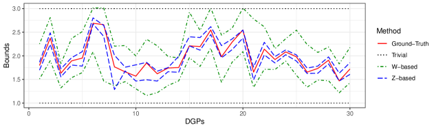
Figure 6: Bounds for the conditional potential outcome mean for 30 random choices of the data generating process. Samples size from each data generating process is $n=5000$.

Table 1: Average bound widths and average confidence interval widths for the $W$-based and $Z$-based methods.

	$Z$-based method		$W$-based method
Sample Size	Avg. Bounds Width	Avg. CI Width	Avg. Bounds Width	Avg. CI Width
3000	0.803	0.978	0.244	0.323
4000	0.704	0.853	0.213	0.280
5000	0.616	0.742	0.200	0.263
6000	0.566	0.677	0.177	0.232
7000	0.531	0.635	0.168	0.220
8000	0.506	0.610	0.162	0.211
9000	0.470	0.560	0.151	0.198

We considered $|\mathcal{U}|=|\mathcal{X}|=|\mathcal{W}|=|\mathcal{Z}|=4$, an outcome variable with $|\mathcal{Y}|=3$, and a binary treatment variable. Table 1 presents the average bound width and the average confidence interval width for the conditional potential outcome mean for the $W$-based and $Z$-based methods, where the average is over 100 iterations (ground-truth value was $1.8$, trivial bounds for the parameter was $[1,3]$). The number of bootstrap replicates in each iteration is $B=500$ and the value of the hyper-parameter $\alpha$ is set to $50$. Notably, the $Z$-based bounds, i.e., the bounds based on Part (b) of Corollary 3, exhibit superior performance compared to the $W$-based bounds, i.e., the bounds based on Part (a) of Corollary 3. One may wonder whether the efficacy of the proposed method is contingent upon fortuitous realizations of the data generating process. Figure 6 serves to dispel this concern by illustrating that such dependence on chance is not observed. In that figure we observe the bounds for the conditional potential outcome mean for 30 random choices of the data generating process.

6.2 Simulation Study 2

Table 2: Average bound width for the $W$-based method.

			$|\mathcal{W}|$
$|\mathcal{U}|$	3	4	5	6	7
3	0.563	0.710	0.801	1.028	1.053
4		0.873	1.014	1.179	1.173
5			1.148	1.213	1.330
6				1.378	1.396
7					1.536

Table 3: Average bound width for the $Z$-based method.

			$|\mathcal{Z}|$
$|\mathcal{U}|$	3	4	5	6	7
3	0.161	0.168	0.194	0.281	0.285
4		0.225	0.253	0.356	0.383
5			0.295	0.360	0.430
6				0.345	0.366
7					0.532

Next we considered the case that $|\mathcal{W}|$ and $|\mathcal{Z}|$ are larger than or equal to $|\mathcal{U}|$. In this case, based on the results of Shi et al., 2020a , the bridge functions $h$ and $q$ exist and hence again the assumptions of Theorems 1 and 2 are satisfied. However, in this case, the bridge functions are not necessarily unique. Additionally, the proxy variables may incorporate information that is not directly pertinent to the latent confounder, resulting in wider bounds. This phenomenon is corroborated by the simulation results depicted in Tables 3 and 3. Each entry of the table is the width of the estimated bound averaged over 100 random data generating processes. The results are for sample size $n=10000$, $|\mathcal{X}|=5$, $|\mathcal{Y}|=3$, and a binary treatment variable.

Table 4: Coverage of the $W$-based and $Z$-based methods bounds for different values of $|\mathcal{W}|=|\mathcal{Z}|$.

		$|\mathcal{W}|=|\mathcal{Z}|$
	3	4	5	6
$W$-based method	98.4%	99.4%	100%	100%
$Z$-based method	62.2%	76.2%	84.4%	92%

6.3 Simulation Study 3

Finally, we considered the case that $|\mathcal{W}|$ and $|\mathcal{Z}|$ are smaller than $|\mathcal{U}|$. We considered $|\mathcal{U}|=7$, $|\mathcal{X}|=5$, $|\mathcal{Y}|=3$, $|\mathcal{W}|=|\mathcal{Z}|\in\{3,4,5,6\}$, and a binary treatment variable. In this case, the bridge functions $h$ and $q$ do not exist and hence, the assumptions of Theorems 1 and 2 are violated. We investigated the coverage of our bounds to study the sensitivity of the approach to the existing slight violation of our assumption. To do so, we looked at 500 random data generating processes and investigated in what percentage of them the bounds obtained from a sample of size 10,000 contain the ground truth. The results are shown in Table 4. The obtained coverages may demonstrate the robustness of our proposed methods to slight violation of the assumption of existence of bridge functions.

7 Evaluation of the Effectiveness of Right Heart Catheterization

In this section, we demonstrate the application of the proposed method to the Study to Understand Prognoses and Preferences for Outcomes and Risks of Treatments (SUPPORT) to evaluation of the effectiveness of right heart catheterization (RHC) in the intensive care unit of critically ill patients (Connors et al.,, 1996). The same dataset has been analyzed using proximal framework in (Tchetgen Tchetgen et al.,, 2020; Cui et al.,, 2023) with parametric estimation on nuisance parameters, and in (Ghassami et al., 2021b, ) with non-parametric estimation of nuisance functions.

Data are available on 5735 individuals, 2184 treated and 3551 controls. In total, 3817 patients survived and 1918 died within 30 days. The binary treatment variable $A$ is whether RHC is assigned, and the outcome variable $Y$ is the number of days between admission and death or censoring at day 30. Based on background knowledge, we included the following five binary pre-treatment covariates to adjust for potential confounding:

• $X_{1}$: Indicator of age above 75;

• $X_{2}$: Indicator of APACHE score above 40;

• $X_{3}$: Indicator of estimate of probability of surviving two months above 0.5;

• $X_{4}$: Indicator that patient has congestive heart failure or acute respiratory failure;

• $X_{5}$: Indicator of hematocrit above 30%.

Based on the superior performance of the $Z$-based method observed in synthetic data evaluations, we only applied that method in our real data analysis. Hence, we only require proxy variable $Z$, for which, following (Tchetgen Tchetgen et al.,, 2020; Cui et al.,, 2023), we considered two options: (1) The status of PaO2/FI02 ratio (PaFI). Specifically, we used the binary variable $Z$ the indicator of PaO2/FI02 ratio above 150. (2) The status of partial pressure of CO2 (PaCO2). Specifically, we used the binary variable $Z$ the indicator of PaCO2 above 37 mmHg. The results are summarized in Table 5. As it can be seen in Table 5, both choices of the proxy variable $Z$ lead to a negative causal effect of RHC on survival. The results are consistent with the previous results in the literature on this dataset. Specifically, that of Cui et al., (2023) (ATE = $-1.66$, 95% confidence interval = $(-2.50,-0.83)$) and Ghassami et al., 2021b (ATE = $-1.70$, 95% confidence interval = $(-2.17,-1.22)$).

Table 5: Causal effect estimates and 95% confidence intervals for two choices of the proxy variable $Z$.

	ATE bounds	95% CIs
PaFI as the proxy variable	$(-2.250,-0.093)$	$(-2.738,0.403)$
PaCO2 as the proxy variable	$(-2.281,-0.038)$	$(-2.721,0.466)$

8 Conclusion

For point identification of causal effects, proximal causal inference requires identification of certain nuisance functions called bridge functions using proxy variables that are sufficiently relevant to the unmeasured confounder, formalized as a completeness condition. However, completeness is not testable, and although a bridge function may exist, lack of completeness may severely limit prospects for identification of a bridge function and thus a causal effect; therefore, restricting the application of the framework. In this work, we proposed partial identification methods that do not require completeness and obviate the need for identification of a bridge function, i.e., we established that proxies can be leveraged to obtain bounds on the causal effect even if available information does not suffice to identify a bridge function. We further established analogous results for mediation analysis when the mediator is unobserved. Since our bounds are non-smooth functionals of the observed data distribution, in the context of inference, we proposed the use of a smooth approximation of our bounds. We provided detailed simulation results to demonstrate the performance of our proposed methods. Specifically, we observed that the $Z$-based method in many settings provide very informative bounds on the causal effect. We also demonstrated the application of our proposed method to the Study to Understand Prognoses and Preferences for Outcomes and Risks of Treatments (SUPPORT) to evaluation of the effectiveness of right heart catheterization in the intensive care unit of critically ill patients. Our results were consistent with the previous findings in the literature on this dataset.

Appendix

Proofs

Proof of Theorem 1.

We note that

$$\mathbb{E}[Y^{(A=a)}\mid A=1-a]$$

$$=\mathbb{E}\Big{[}\mathbb{E}[Y^{(A=a)}\mid A=a,X,U]\Big{|}A=1-a\Big{]}$$

$$\overset{(a)}{=}\mathbb{E}\Big{[}\mathbb{E}[Y\mid A=a,X,U]\Big{|}A=1-a\Big{]}$$

$$\overset{(b)}{=}\mathbb{E}\Big{[}\mathbb{E}[h(W,a,X)\mid A=a,X,U]\Big{|}A=1-a\Big{]}$$

$$\overset{(c)}{=}\mathbb{E}\Big{[}\mathbb{E}[h(W,a,X)\mid A=1-a,X,U]\Big{|}A=1-a\Big{]}$$

$$=\mathbb{E}\Big{[}h(W,a,X)\Big{|}A=1-a\Big{]}$$

$$=\sum_{w,x}h(w,a,x)\frac{p(w\mid A=1-a,x)}{p(w\mid A=a,x)}p(w\mid A=a,x)p(x\mid A=1-a),$$

where $(a)$ is due to the consistency assumption, $(b)$ is due to Assumption 2, and $(c)$ is due to Assumption 1. Therefore,

$$\sum_{x}\min_{w}\frac{p(w\mid A=1-a,x)}{p(w\mid A=a,x)}\sum_{w}h(w,a,x)p(w\mid A=a,x)p(x\mid A=1-a)$$

$$\leq\mathbb{E}[Y^{(A=a)}\mid A=1-a]\leq$$

$$\sum_{x}\max_{w}\frac{p(w\mid A=1-a,x)}{p(w\mid A=a,x)}\sum_{w}h(w,a,x)p(w\mid A=a,x)p(x\mid A=1-a).$$

Note that Assumption 2 implies that almost surely

$$\mathbb{E}[Y\mid A=a,X]=\mathbb{E}[h(W,a,X)\mid A=a,X].$$

Therefore,

$$\sum_{x}\min_{w}\frac{p(w\mid A=1-a,x)}{p(w\mid A=a,x)}\sum_{y}yp(y\mid A=a,x)p(x\mid A=1-a)$$

$$\leq\mathbb{E}[Y^{(A=a)}\mid A=1-a]\leq$$

$$\sum_{x}\max_{w}\frac{p(w\mid A=1-a,x)}{p(w\mid A=a,x)}\sum_{y}yp(y\mid A=a,x)p(x\mid A=1-a).$$

Combining the above bounds with the trivial bounds that $\inf\mathcal{Y}\leq\mathbb{E}[Y^{(A=a)}\mid A=1-a]\leq\sup\mathcal{Y}$ leads to the desired result.

∎

Proof of Corollary 1.

We note that

$$\mathbb{E}[Y^{(a)}]=\mathbb{E}[Y^{(a)}\mid A=1-a]p(A=1-a)+\mathbb{E}[Y^{(a)}\mid A=a]p(A=a).$$

Therefore, the following concludes the upper bound in the corollary.

$$\sum_{x}\max_{w}\frac{p(w\mid A=1-a,x)}{p(w\mid A=a,x)}\sum_{y}yp(y\mid A=a,x)p(x\mid A=1-a)p(A=1-a)$$

$$\qquad+\mathbb{E}[Y\mid A=a]p(A=a)$$

$$=\sum_{x}\max_{w}\frac{p(A=1-a\mid w,x)}{p(A=a\mid w,x)}\frac{p(A=a\mid x)}{p(A=1-a\mid x)}\sum_{y}yp(y\mid A=a,x)p(x\mid A=1-a)p(A=1-a)$$

$$\qquad+\mathbb{E}[Y\mid A=a]p(A=a)$$

$$=\sum_{x}\max_{w}\frac{p(A=1-a\mid w,x)}{p(A=a\mid w,x)}\sum_{y}yp(y\mid A=a,x)p(x,A=a)+\mathbb{E}[Y\mid A=a]p(A=a)$$

$$=\sum_{x}\Big{\{}1+\max_{w}\frac{p(A=1-a\mid w,x)}{p(A=a\mid w,x)}\Big{\}}\sum_{y}yp(y,A=a,x)$$

$$=\sum_{x}\Big{\{}1+\max_{w}\frac{1}{p(A=a\mid w,x)}-1\Big{\}}\sum_{y}yp(y,A=a,x)$$

$$=\sum_{x}\max_{w}\frac{1}{p(A=a\mid w,x)}\sum_{y}yp(y,A=a,x),$$

The lower bound can be proved similarly.

∎

Proof of Theorem 2.

We note that

$$\mathbb{E}\big{[}Y^{(A=a)}\mid A=1-a]$$

$$=\mathbb{E}\big{[}\mathbb{E}[Y^{(A=a)}\mid A=a,X,U]\mid A=1-a\big{]}$$

$$\overset{(a)}{=}\mathbb{E}\big{[}\mathbb{E}[Y\mid A=a,X,U]\mid A=1-a\big{]}$$

$$=\sum_{y,x,u}yp(y\mid A=a,x,u)\frac{p(u\mid x,A=1-a)}{p(u\mid x,A=a)}\frac{p(x\mid A=1-a)}{p(x\mid A=a)}p(x,u\mid A=a)$$

$$\overset{(b)}{=}\sum_{z,y,x,u}yq(z,a,x)p(y\mid a,x,u)p(z\mid a,x,u)\frac{p(x\mid A=1-a)}{p(x\mid A=a)}p(x,u\mid A=a)$$

$$\overset{(c)}{=}\sum_{z,y,x,u}yq(z,a,x)p(z,y,x,u\mid A=a)\frac{p(x\mid A=1-a)}{p(x\mid A=a)}$$

$$=\sum_{z,y,x}yq(z,a,x)p(z,y\mid x,A=a)p(x\mid A=1-a)$$

$$=\sum_{z,x}\mathbb{E}[Y\mid A=a,z,x]q(z,a,x)p(z\mid x,A=a)p(x\mid A=1-a),$$

where $(a)$ is due to the consistency assumption, $(b)$ is due to Assumption 5, and $(c)$ is due to Assumption 4. Therefore,

$$\sum_{x}\min_{z}\mathbb{E}[Y\mid z,x,A=a]\sum_{z}q(z,a,x)p(z\mid A=a,x)p(x\mid A=1-a)$$

$$\leq\mathbb{E}\big{[}Y^{(A=a)}\mid A=1-a]\leq$$

$$\sum_{x}\max_{z}\mathbb{E}[Y\mid z,x,A=a]\sum_{z}q(z,a,x)p(z\mid A=a,x)p(x\mid A=1-a).$$

Note that Assumption 5 implies that almost surely

$$\mathbb{E}[q(Z, A,X)\mid A,X]$$

$$=\sum_{u}\mathbb{E}[q(Z,A,X)\mid A,X,u]p(u\mid A,X)=\sum_{u}p(u\mid 1-A,X)=1.$$

Therefore,

$$\sum_{x}\min_{z}\mathbb{E}[Y\mid z,x,A=a]p(x\mid A=1-a)$$

$$\leq\mathbb{E}\big{[}Y^{(A=a)}\mid A=1-a]\leq$$

$$\sum_{x}\max_{z}\mathbb{E}[Y\mid z,x,A=a]p(x\mid A=1-a).$$

∎

Proof of Theorem 3.

We note that

$$\mathbb{E}[Y^{(A=a)}\mid A=1-a]$$

$$\overset{(a)}{=}\sum_{y,x,u}yp(y\mid a,x,u)p(x,u\mid A=1-a)$$

$$\overset{(b)}{=}\sum_{w,x,u}h(w,a,x)p(w\mid a,x,u)p(x,u\mid A=1-a)$$

$$=\sum_{w,x,u}h(w,a,x)p(w\mid a,x,u)\frac{p(u\mid A=1-a,x)}{p(u\mid A=a,x)}\frac{p(x\mid A=1-a)}{p(x\mid A=a)}p(x,u\mid A=a)$$

$$\overset{(c)}{=}\sum_{w,z,x,u}h(w,a,x)q(z,a,x)p(w\mid a,x,u)p(z\mid a,x,u)\frac{p(x\mid A=1-a)}{p(x\mid A=a)}p(x,u\mid A=a)$$

$$\overset{(d)}{=}\sum_{w,z,x,u}h(w,a,x)q(z,a,x)p(w,z\mid a,x,u)\frac{p(x\mid A=1-a)}{p(x\mid A=a)}p(x,u\mid A=a)$$

$$=\sum_{w,z,x}h(w,a,x)q(z,a,x)p(w,z\mid a,x)p(x\mid A=1-a),$$

where $(a)$ is due to Assumption 3, $(b)$ is due to Assumption 2, $(c)$ is due to Assumption 5. and $(d)$ is due to Assumption 6. Therefore,

$$\sum_{x}\min_{w,z}\frac{p(w,z\mid a,x)}{p(w\mid a,x)p(z\mid a,x)}\sum_{w}h(w,a,x)p(w\mid a,x)\sum_{z}q(z,a,x)p(z\mid a,x)p(x\mid A=1-a)$$

$$\leq\mathbb{E}[Y^{(A=a)}\mid A=1-a]\leq$$

$$\sum_{x}\max_{w,z}\frac{p(w,z\mid a,x)}{p(w\mid a,x)p(z\mid a,x)}\sum_{w}h(w,a,x)p(w\mid a,x)\sum_{z}q(z,a,x)p(z\mid a,x)p(x\mid A=1-a).$$

Note that

$$\sum_{w}h(w,a,x)p(w\mid a,x)=\sum_{y}yp(y\mid a,x),$$

and

$$\sum_{z}q(z,a,x)p(z\mid a,x)=1.$$

Therefore,

$$\mathbb{E}\Big{[}\min_{w,z}\frac{p(w,z\mid a,X)}{p(w\mid a,X)p(z\mid a,X)}\mathbb{E}[Y\mid A=a,X]\Big{|}A=1-a\Big{]}$$

$$\leq\mathbb{E}[Y^{(A=a)}\mid A=1-a]\leq$$

$$\mathbb{E}\Big{[}\max_{w,z}\frac{p(w,z\mid a,X)}{p(w\mid a,X)p(z\mid a,X)}\mathbb{E}[Y\mid A=a,X]\Big{|}A=1-a\Big{]}.$$

Combining the above bounds with the trivial bounds that $\inf\mathcal{Y}\leq\mathbb{E}[Y^{(A=a)}\mid A=1-a]\leq\sup\mathcal{Y}$ leads to the desired result. ∎

Proof of Theorem 4.

We note that

$$\mathbb{E}[Y^{(1,M^{(0)})}]$$

$$=\mathbb{E}\Big{[}\mathbb{E}\big{[}\mathbb{E}[Y\mid A=1,X,M]\big{|}A=0,X\big{]}\Big{]}$$

$$=\mathbb{E}\Big{[}\mathbb{E}\big{[}\mathbb{E}[h(W,X)\mid X,M]\big{|}A=0,X\big{]}\Big{]}$$

$$=\mathbb{E}\Big{[}\mathbb{E}\big{[}\mathbb{E}[h(W,X)\mid A=0,X,M]\big{|}A=0,X\big{]}\Big{]}$$

$$=\mathbb{E}\Big{[}\mathbb{E}[h(W,X)\mid A=0,X]\Big{]}$$

$$=\mathbb{E}\Big{[}\mathbb{E}[\frac{p(W\mid A=0,X)}{p(W\mid A=1,X)}h(W,X)\mid A=1,X]\Big{]}.$$

Therefore,

$$\mathbb{E}\Big{[}\min_{w}\frac{p(w\mid A=0,X)}{p(w\mid A=1,X)}\mathbb{E}[h(W,X)\mid A=1,X]\Big{]}$$

$$\leq\mathbb{E}[Y^{(1,M^{(0)})}]\leq$$

$$\mathbb{E}\Big{[}\max_{w}\frac{p(w\mid A=0,X)}{p(w\mid A=1,X)}\mathbb{E}[h(W,X)\mid A=1,X]\Big{]}.$$

Note that Assumption 10 implies that almost surely

$$\mathbb{E}[Y\mid A=1,X]=\mathbb{E}[h(W,X)\mid A=1,X].$$

Therefore,

$$\mathbb{E}\Big{[}\min_{w}\frac{p(w\mid A=0,X)}{p(w\mid A=1,X)}\mathbb{E}[Y\mid A=1,X]\Big{]}$$

$$\leq\mathbb{E}[Y^{(1,M^{(0)})}]\leq$$

$$\mathbb{E}\Big{[}\max_{w}\frac{p(w\mid A=0,X)}{p(w\mid A=1,X)}\mathbb{E}[Y\mid A=1,X]\Big{]}.$$

Combining the above bounds with the trivial bounds that $\inf\mathcal{Y}\leq\mathbb{E}[Y^{(1,M^{(0)})}]\leq\sup\mathcal{Y}$ leads to the desired result.

∎

Proof of Theorem 5.

We note that

$$\mathbb{E}[Y^{(A=a)}]$$

$$=\mathbb{E}[I(A=a)Y]+\sum_{m,y,x}yp(y\mid A=1-a,m,x)p(m\mid A=a,x)p(A=1-a\mid x)p(x)$$

$$=\mathbb{E}[I(A=a)Y]+\sum_{m,w,x}h(w,1-a,x)p(w\mid 1-a,m,x)p(m\mid a,x)p(1-a\mid x)p(x)$$

$$=\mathbb{E}[I(A=a)Y]+\sum_{m,w,x}h(w,1-a,x)p(w\mid a,m,x)p(m\mid a,x)p(1-a\mid x)p(x)$$

$$=\mathbb{E}[I(A=a)Y]+\sum_{w,x}h(w,1-a,x)p(w\mid a,x)p(1-a\mid x)p(x)$$

$$=\mathbb{E}[I(A=a)Y]+\sum_{w,x}\frac{p(w\mid a,x)}{p(w\mid 1-a,x)}h(w,1-a,x)p(w\mid 1-a,x)p(1-a\mid x)p(x).$$

Therefore,

$$\mathbb{E}[I(A=a)Y]+\sum_{x}\min_{w}\frac{p(w\mid a,x)}{p(w\mid 1-a,x)}\sum_{w}h(w,1-a,x)p(w\mid 1-a,x)p(1-a\mid x)p(x)$$

$$\leq\mathbb{E}[Y^{(A=a)}]\leq$$

$$\mathbb{E}[I(A=a)Y]+\sum_{x}\max_{w}\frac{p(w\mid a,x)}{p(w\mid 1-a,x)}\sum_{w}h(w,1-a,x)p(w\mid 1-a,x)p(1-a\mid x)p(x).$$

Note that Assumption 12 implies that almost surely

$$\mathbb{E}[Y\mid A,X]=\mathbb{E}[h(W,A,X)\mid A,X].$$

Therefore,

$$\mathbb{E}[I(A=a)Y]+\sum_{x,y}\min_{w}\frac{p(w\mid a,x)}{p(w\mid 1-a,x)}yp(y,1-a,x)$$

$$\leq\mathbb{E}[Y^{(A=a)}]\leq$$

$$\mathbb{E}[I(A=a)Y]+\sum_{x,y}\max_{w}\frac{p(w\mid a,x)}{p(w\mid 1-a,x)}yp(y,1-a,x),$$

Combining the above bounds with the trivial bounds based on the support of $Y$ leads to the desired result.

∎

References

- Bennett et al., (2023) Bennett, A., Kallus, N., Mao, X., Newey, W., Syrgkanis, V., and Uehara, M. (2023). Minimax instrumental variable regression and convergence guarantees without identification or closedness. arXiv preprint arXiv:2302.05404.
- Boyd and Vandenberghe, (2004) Boyd, S. P. and Vandenberghe, L. (2004). Convex optimization. Cambridge university press.
- Calafiore et al., (2019) Calafiore, G. C., Gaubert, S., and Possieri, C. (2019). Log-sum-exp neural networks and posynomial models for convex and log-log-convex data. IEEE transactions on neural networks and learning systems, 31(3):827–838.
- Calafiore et al., (2020) Calafiore, G. C., Gaubert, S., and Possieri, C. (2020). A universal approximation result for difference of log-sum-exp neural networks. IEEE transactions on neural networks and learning systems, 31(12):5603–5612.
- Chernozhukov et al., (2012) Chernozhukov, V., Chetverikov, D., and Kato, K. (2012). Central limit theorems and multiplier bootstrap when p is much larger than n. Technical report, cemmap working paper.
- Connors et al., (1996) Connors, A. F., Speroff, T., Dawson, N. V., Thomas, C., Harrell, F. E., Wagner, D., Desbiens, N., Goldman, L., Wu, A. W., Califf, R. M., et al. (1996). The effectiveness of right heart catheterization in the initial care of critically iii patients. Jama, 276(11):889–897.
- Cui et al., (2023) Cui, Y., Pu, H., Shi, X., Miao, W., and Tchetgen Tchetgen, E. (2023). Semiparametric proximal causal inference. Journal of the American Statistical Association, pages 1–12.
- Deaner, (2018) Deaner, B. (2018). Proxy controls and panel data. arXiv preprint arXiv:1810.00283.
- Dukes et al., (2023) Dukes, O., Shpitser, I., and Tchetgen Tchetgen, E. J. (2023). Proximal mediation analysis. Biometrika.
- Egami and Tchetgen Tchetgen, (2023) Egami, N. and Tchetgen Tchetgen, E. J. (2023). Identification and estimation of causal peer effects using double negative controls for unmeasured network confounding. Journal of the Royal Statistical Society Series B: Statistical Methodology.
- Ghassami et al., (2022) Ghassami, A., Yang, A., Richardson, D., Shpitser, I., and Tchetgen Tchetgen, E. (2022). Combining experimental and observational data for identification of long-term causal effects. arXiv preprint arXiv:2201.10743.
- (12) Ghassami, A., Yang, A., Shpitser, I., and Tchetgen Tchetgen, E. (2021a). Causal inference with hidden mediators. arXiv preprint arXiv:2111.02927.
- (13) Ghassami, A., Ying, A., Shpitser, I., and Tchetgen, E. T. (2021b). Minimax kernel machine learning for a class of doubly robust functionals. arXiv preprint arXiv:2104.02929.
- Goodfellow et al., (2016) Goodfellow, I., Bengio, Y., and Courville, A. (2016). Deep learning. MIT press.
- Hernán and Robins, (2020) Hernán, M. A. and Robins, J. M. (2020). Causal inference: what if.
- Imai et al., (2010) Imai, K., Keele, L., and Tingley, D. (2010). A general approach to causal mediation analysis. Psychological methods, 15(4):309.
- Levis et al., (2023) Levis, A. W., Bonvini, M., Zeng, Z., Keele, L., and Kennedy, E. H. (2023). Covariate-assisted bounds on causal effects with instrumental variables. arXiv preprint arXiv:2301.12106.
- Li et al., (2023) Li, K. Q., Shi, X., Miao, W., and Tchetgen Tchetgen, E. (2023). Double Negative Control Inference in Test-Negative Design Studies of Vaccine Effectiveness. Journal of the American Statistical Association: Theory and Methods.
- Lipsitch et al., (2010) Lipsitch, M., Tchetgen Tchetgen, E., and Cohen, T. (2010). Negative controls: a tool for detecting confounding and bias in observational studies. Epidemiology (Cambridge, Mass.), 21(3):383.
- (20) Miao, W., Geng, Z., and Tchetgen Tchetgen, E. J. (2018a). Identifying causal effects with proxy variables of an unmeasured confounder. Biometrika, 105(4):987–993.
- (21) Miao, W., Shi, X., and Tchetgen Tchetgen, E. (2018b). A confounding bridge approach for double negative control inference on causal effects. arXiv preprint arXiv:1808.04945.
- Murphy, (2012) Murphy, K. P. (2012). Machine learning: a probabilistic perspective. MIT press.
- Pearl, (2001) Pearl, J. (2001). Direct and indirect effects. In Proceedings of the 17th Conference on Uncertainty in Artificial Intelligence (pp. 411– 420).
- Pearl, (2009) Pearl, J. (2009). Causality. Cambridge university press.
- Robins and Greenland, (1992) Robins, J. M. and Greenland, S. (1992). Identifiability and exchangeability for direct and indirect effects. Epidemiology, pages 143–155.
- (26) Shi, X., Miao, W., Nelson, J. C., and Tchetgen Tchetgen, E. J. (2020a). Multiply robust causal inference with double-negative control adjustment for categorical unmeasured confounding. Journal of the Royal Statistical Society: Series B (Statistical Methodology), 82(2):521–540.
- (27) Shi, X., Miao, W., and Tchetgen Tchetgen, E. (2020b). A selective review of negative control methods in epidemiology. Current epidemiology reports, 7:190–202.
- Shpitser et al., (2023) Shpitser, I., Wood-Doughty, Z., and Tchetgen Tchetgen, E. J. (2023). The proximal ID algorithm. Journal of Machine Learning Research.
- Tchetgen Tchetgen et al., (2023) Tchetgen Tchetgen, E., Park, C., and Richardson, D. (2023). Single proxy control. arXiv preprint arXiv:2302.06054.
- Tchetgen Tchetgen and Wirth, (2017) Tchetgen Tchetgen, E. J. and Wirth, K. E. (2017). A general instrumental variable framework for regression analysis with outcome missing not at random. Biometrics, 73(4):1123–1131.
- Tchetgen Tchetgen et al., (2020) Tchetgen Tchetgen, E. J., Ying, A., Cui, Y., Shi, X., and Miao, W. (2020). An introduction to proximal causal learning. arXiv preprint arXiv:2009.10982.
- Wainwright, (2019) Wainwright, M. J. (2019). High-dimensional statistics: A non-asymptotic viewpoint, volume 48. Cambridge University Press.
- Ying et al., (2023) Ying, A., Miao, W., Shi, X., and Tchetgen Tchetgen, E. J. (2023). Proximal causal inference for complex longitudinal studies. Journal of the Royal Statistical Society Series B: Statistical Methodology.
- Zhang et al., (2023) Zhang, J., Li, W., Miao, W., and Tchetgen Tchetgen, E. (2023). Proximal causal inference without uniqueness assumptions. Statistics & Probability Letters, page 109836.