Morse inequalities for ordered eigenvalues of generic self-adjoint families
Abstract.
In many applied problems one seeks to identify and count the critical points of a particular eigenvalue of a smooth parametric family of self-adjoint matrices, with the parameter space often being known and simple, such as a torus. Among particular settings where such a question arises are the Floquet–Bloch decomposition of periodic Schrödinger operators, topology of potential energy surfaces in quantum chemistry, spectral optimization problems such as minimal spectral partitions of manifolds, as well as nodal statistics of graph eigenfunctions. In contrast to the classical Morse theory dealing with smooth functions, the eigenvalues of families of self-adjoint matrices are not smooth at the points corresponding to repeated eigenvalues (called, depending on the application and on the dimension of the parameter space, the diabolical/Dirac/Weyl points or the conical intersections).
This work develops a procedure for associating a Morse polynomial to a point of eigenvalue multiplicity; it utilizes the assumptions of smoothness and self-adjointness of the family to provide concrete answers. In particular, we define the notions of non-degenerate topologically critical point and generalized Morse family, establish that generalized Morse families are generic in an appropriate sense, establish a differential first-order conditions for criticality, as well as compute the local contribution of a topologically critical point to the Morse polynomial. Remarkably, the non-smooth contribution to the Morse polynomial turns out to be universal: it depends only on the size of the eigenvalue multiplicity and the relative position of the eigenvalue of interest and not on the particulars of the operator family; it is expressed in terms of the homologies of Grassmannians.
Key words and phrases:
Dirac points, Weyl points, diabolical points, conical intersections, operator-valued functions, Morse inequalities, Clarke subdifferential, homology of Grassmannians, stratified Morse theory2020 Mathematics Subject Classification:
47A56, 47A10, 57R70, 58K05, 49J52, 14M15, 58A35, 57Z051. Introduction
Let and denote the spaces of real symmetric (correspondingly, complex Hermitian) matrices. When referring to both spaces at once, we will use the term “self-adjoint matrices” and use the notation . The eigenvalues of a matrix are real and will be numbered in the increasing order,
| (1.1) |
Further, let be a smooth (i.e. ) compact -dimensional manifold. A smooth -parametric family of self-adjoint matrices (on ) is a smooth map from to .
The aim of this paper is to develop the Morse theory for the -th eigenvalue branch
| (1.2) |
viewed as a function on . This question is motivated by numerous problems in mathematical physics. The boundaries between isolating and conducting regimes in a periodic (crystalline) structure are determined by the extrema of eigenvalues of an operator111The particulars of the operator depend on what is being conducted: electrons, light, sound, etc. family defined on a -dimensional torus (for an introduction to the mathematics of this subject, see [K16]). Other critical points of the eigenvalues give rise to special physically observable features of the density of states, the van Hove singularities [VH53]. Classifying all critical points of an eigenvalue (also on a torus) by their degree is used to study oscillation of eigenfunctions via the nodal–magnetic theorem [B13, CdV13, AG22]. More broadly, the area of eigenvalue optimization encompasses questions from understanding the charge distribution in an atomic nucleus [ELS21], configuration of atoms in a polyatomic molecule [DYK04, M21], to shape optimization [H06, H17b] and optimal partition of domains and networks [HHO13, BBRS12]. The dimension of the manifold in these applications can be very high or even infinite.
Morse theory is a natural tool for connecting statistics of the critical points with the topology of the underlying manifold. However, the classical Morse theory is formulated for functions that are sufficiently smooth, whereas the function is generically non-smooth at the points where is a repeated eigenvalue of the matrix . And it is these points of non-smoothness that play an outsized role in the applications [CNGP+09, DYK04].
By Bronstein’s theorem [B79], each is Lipschitz. Furthermore, by classical perturbation theory [K95], the function is smooth along a submanifold if the multiplicity of is constant on ; the latter property induces a stratification of . There exist generalizations of Morse theory to Lipschitz functions (see, for example, [APS97], [FF89, §45]) as well as to stratified spaces [GM88]. These generalizations will provide the general foundation for our work, but the principal thrust of this paper is to leverage the properties of and to get explicit — and beautiful — answers for the Morse data in terms of the local behavior of at a discrete set of points we will identify as “critical”. One of the surprising findings is that the Morse data attributable to the non-smooth directions at a critical point has a universal form.
To set the stage for our results we now review informally the main ideas of Morse theory. Let be Lipschitz and define the sublevel set
| (1.3) |
and, for an open set , the local sublevel set,
| (1.4) |
Generally speaking, Morse theory studies the change in the homotopy type of as increases. If is smooth, this change can be explicitly described in terms of the critical points of and their indices in the differential sense. As a result, the topological invariants of the manifold itself, such as the Betti numbers, are related to these indices via the Morse inequalities.
In more detail, if is smooth, a point is called a critical point if the differential of vanishes at . The Hessian (second differential) of at is a quadratic form on the tangent space . In local coordinates it is represented by the matrix of second derivatives, the Hessian matrix. The Morse index of is defined as the negative index of this quadratic form or, equivalently, the number of negative eigenvalues of the Hessian matrix. It is assumed that the second differential at every critical point of is non-singular, i.e. the Hessian matrix has no zero eigenvalues; such critical points are called non-degenerate. Non-degenerate critical points are isolated and therefore there are only finitely many of them on . A smooth function is called a Morse function if all its critical points are non-degenerate.
The first main result of the classical Morse theory states that if is a non-degenerate critical point of index , then, for a sufficiently small neighborhood of and sufficiently small , the space is homotopy equivalent to the -dimensional sphere . The global consequences of this are as follows. One defines the Morse polynomial of a Morse function as the sum of over all critical points of . On the topological side, the Poincaré polynomial of the manifold is the sum of , where is the -th Betti number of the manifold , defined as the rank of the homology group . The Morse inequalities encode the relationship between the number of critical points of on and the Betti numbers of in the following form:
| (1.5) |
where is a polynomial with nonnegative coefficients. To put it another way, the Betti numbers give the lower bound for the number of critical points of index ; extra critical points can only be created in pairs of adjacent index.
Now assume that is just continuous. Mimicking the classical Morse theory of smooth functions we adopt the following definitions (cf. [FF89, §45, Def. 1, 2 and 3], the critical points are called bifurcation points there):
Definition 1.1.
A point is a topologically regular point of a continuous function if there exists a neighborhood of in and such that is a strong deformation retract of . We say that a point is topologically critical if it is not topologically regular.
Remark 1.2.
If is smooth, a topologically critical point is also critical in the usual (differential) sense. The converse is, in general, not true: for example, if and , then is critical but not topologically critical. On the other hand, by the aforementioned main result of the classical Morse theory, if is a non-degenerate critical point then it is also topologically critical.
Definition 1.3.
Given a continuous function with a finite set of topologically critical points, the Morse polynomial is the sum, over the topologically critical points , of the Poincaré polynomials of the relative homology groups , where is a small neighborhood of and is sufficiently small.
Note that in the case when is a smooth Morse function, Definition 1.3 reduces to the classical one as the relative homology groups coincide with the reduced homology groups of the -dimensional sphere , where is the Morse index of , and so the contribution of to the Morse polynomial is equal to .
With Definitions 1.1 and 1.3, the Morse inequalities (1.5) hold true for continuous functions with finite number of topologically critical points (see, e.g., [FF89, §45, Theorem. 1]). It is thus our goal to calculate explicitly the Poincaré polynomial under some natural assumptions on the family of self-adjoint matrices. To that end we will need to:
-
(1)
Provide an explicit characterization of non-smooth topologically critical and topologically regular points of ;
-
(2)
Give a natural definition of a non-degenerate non-smooth topologically critical point;
-
(3)
For a non-degenerate topologically critical point of , find the relative homology
for a sufficiently small neighborhood of and sufficiently small . As a by-product, this will determine the correct contribution from to the Morse polynomial of .
We remark that these questions are local in character and we do not need to enforce compactness of while answering them.
In this work, we completely implement the above objectives in the case of generic families; additionally, our sufficient condition for a regular point is obtained for arbitrary families. The first objective is accomplished in the form of a “first derivative test”, with the derivative being applied to the smooth object: the family (see equation (1.7) and Theorems 1.5 and 1.10 for details).
The Morse contribution of a critical point (third objective) will consist of two parts: the classical index of the Hessian of in the directions of smoothness of and a contribution from the non-smooth directions which, remarkably, turns out to be universal. Theorem 1.17 expresses these universal contributions in terms of homologies of suitable Grassmannians; explicit formulas for the Poincaré polynomial are also provided. In section 1.3 we mention some simple practical corollaries of our results as well as pose further problems.
1.1. A differential characterization of topologically critical points of an eigenvalue branch
We start with a simple motivating example.
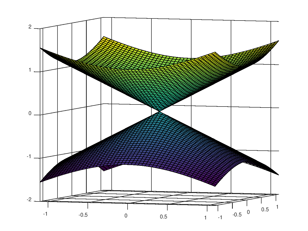
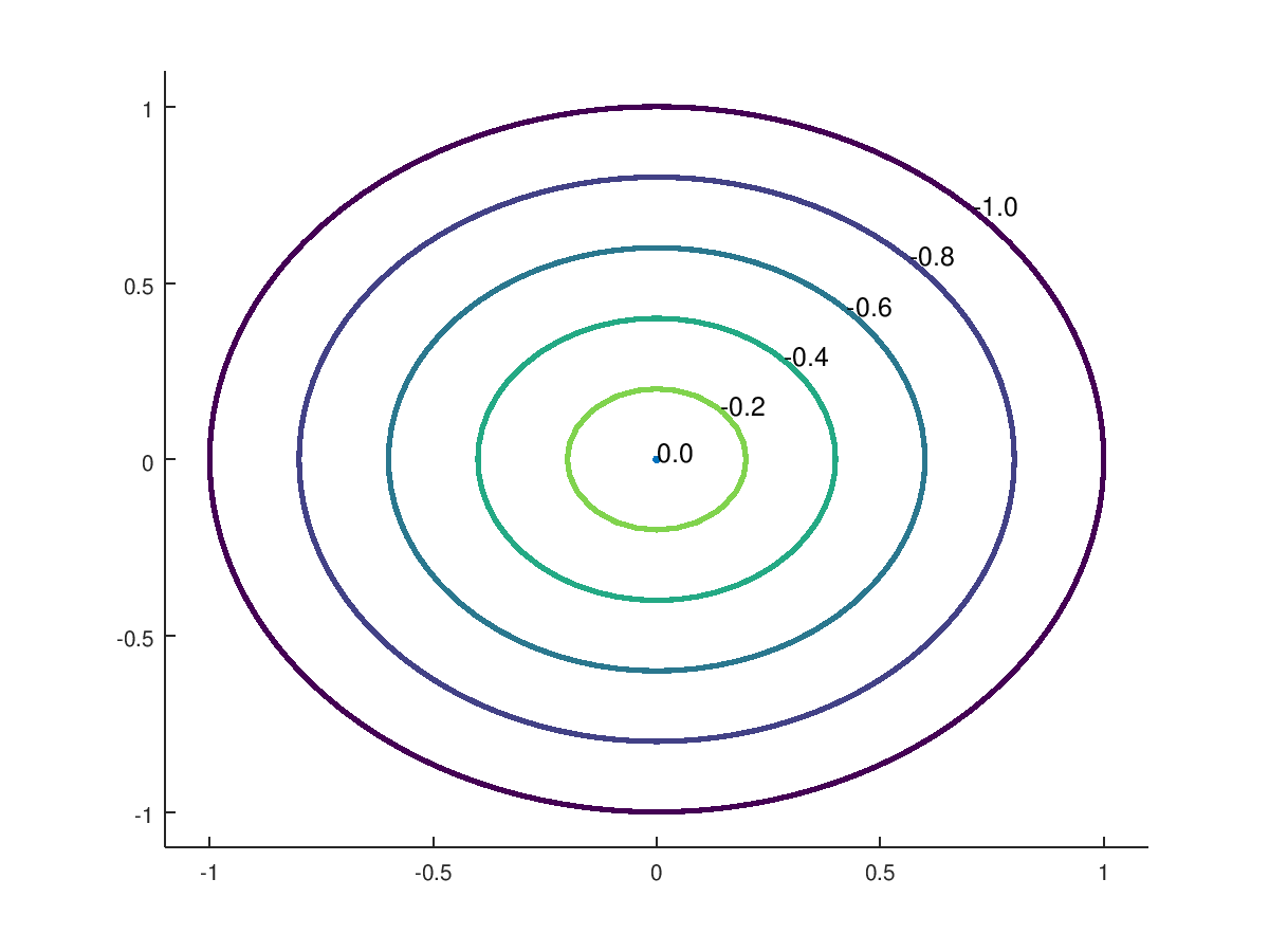
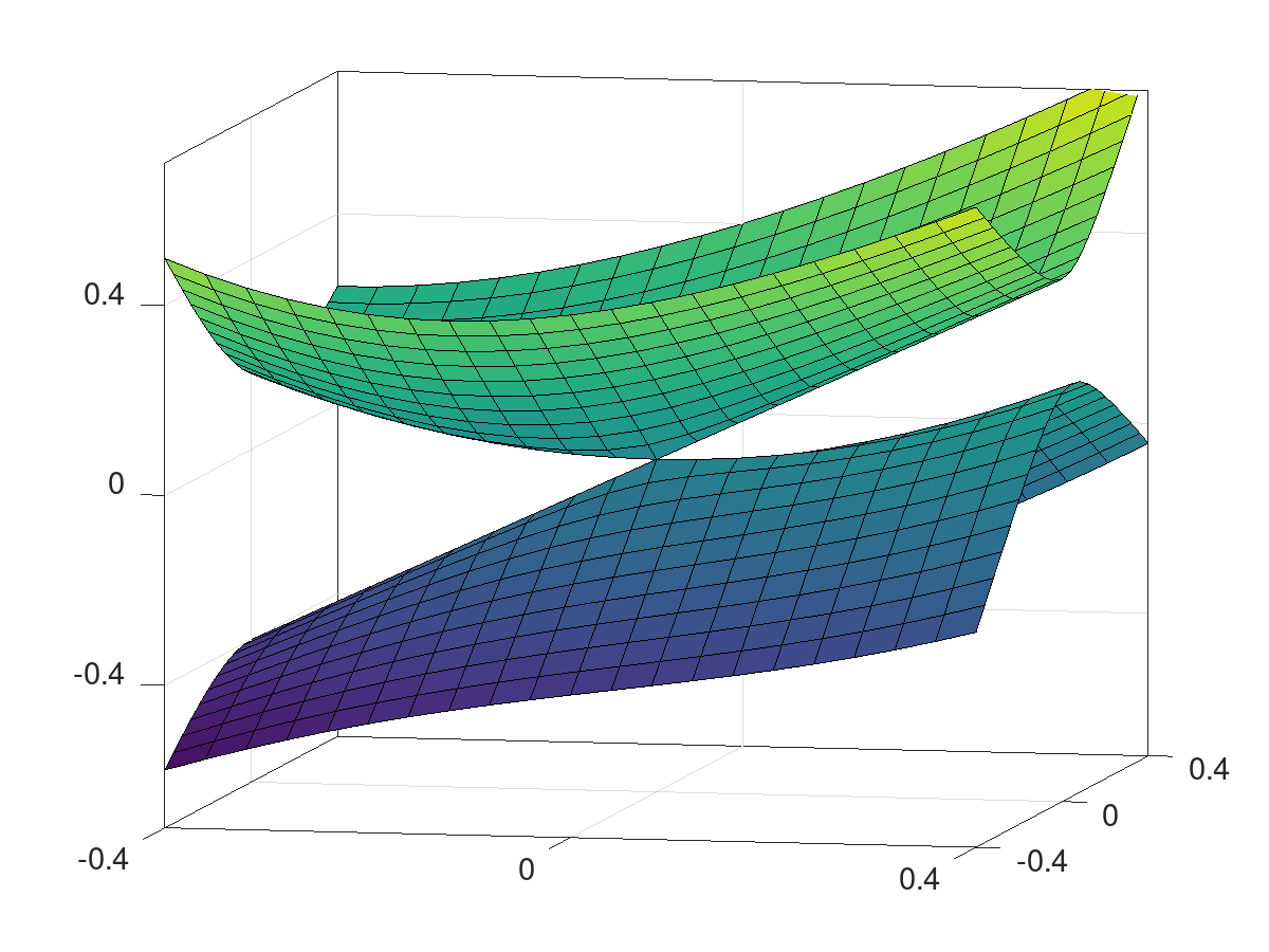
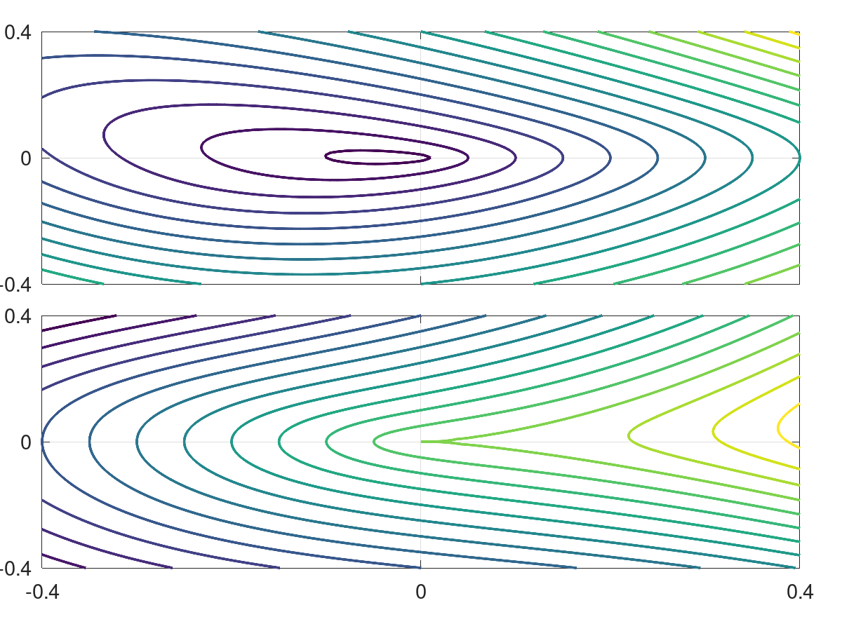
Example 1.4.
Consider the two families
| (1.6) |
Both families and have an isolated point of multiplicity 2 at . Focusing on the lower eigenvalue , its level curves in the case of undergo a significant change at the value — they change from circles to empty, see Fig. 1(top). Therefore, the point is topologically critical and, visually, of has a maximum at . In contrast, the level curves and the sublevel sets of remain homotopically equivalent, see Fig. 1(bottom). The point is not topologically critical for of .
How can we determine efficiently whether a point is topologically regular or critical, especially in higher dimensions where visually inspecting eigenvalue plots is not an option?
We now describe the answer to this question. Denote by the eigenspace of at a point of multiplicity . Let be a linear isometry from to such that (explicitly, the columns of are an orthonormal basis of ). Let denote the linear operator acting as
| (1.7) |
While the operator depends on the choice of basis in , we will only use its properties that are invariant under unitary conjugation. We remark that by what is sometimes called Hellmann–Feynman theorem (see Appendix A and references therein), the eigenvalues of give the slopes of the branches splitting off from the multiple eigenvalue when we leave in the direction .
We recall that a matrix is positive semidefinite (notation: ) if all of its eigenvalues are non-negative, positive definite (notation: ) if all eigenvalues are strictly positive. We denote by the orthogonal complement of a space in with respect to the Frobenius inner product
| (1.8) |
Theorem 1.5.
Let be a smooth family whose eigenvalue has multiplicity at the point . If contains a positive definite matrix or, equivalently,
| (1.9) |
then is topologically regular for .
This theorem is proved in section 2 by studying the Clarke subdifferential at the point . We formulate the conditions in terms of both and because the former emerges naturally from the proof while the latter is simpler in practical computations: generically it is one- or zero-dimensional as we will explain below.
Example 1.6.
Example 1.7.
Condition (1.9) should be viewed as being analogous to the “non-vanishing gradient” in the smooth Morse theory. To illustrate this point, consider the special case when the eigenvalue is smooth. Let be the eigenvector corresponding to at the point . The operator in this case maps to which is equal to the directional derivative of in the direction . The condition of Theorem 1.5 is precisely that this derivative is non-zero in some direction.
Due to the topological nature of Definition 1.1, one cannot expect that a zero gradient-type condition alone would be sufficient for topological criticality (cf. Remark 1.2). To formulate a sufficient condition we need some notion of “non-degeneracy”.
Definition 1.8.
We say that a family is transversal (with respect to eigenvalue ) at a point if
| (1.10) |
where is the multiplicity of at the point and is the space of multiples of the identity matrix.
In section 3 (Lemma 3.1) we will see that this condition is equivalent to the usual differential-topological notion of transversality of the family with the corresponding strata of the discriminant variety, i.e. the subset of consisting of matrices with repeated eigenvalues. Furthermore, in Theorem 3.9, we will show that the set of all families which are transversal at every point is generic (i.e., open and dense) in the Whitney topology in for .
Definition 1.9.
The submanifold is called the (local) constant multiplicity stratum attached to if and, for any in a small neighborhood of in , the multiplicity of is equal to if and only if .
In Corollary 3.3 we will show that condition (1.10) implies the constant multiplicity stratum at is well-defined, has codimension in , where
| (1.11) |
and that the function restricted to is smooth. In particular, the transversality condition (1.10) yields a bound (via ) on the maximal multiplicity of an eigenvalue, which is known as the von Neumann–Wigner theorem [vNW29]. In the borderline case , the manifold is the isolated point (as in Example 1.4).
It is easy to show, see Lemma 3.4, that the converse of condition (1.9) implies that the point is smooth critical for the restriction of to the constant multiplicity stratum attached to , i.e. . Establishing that a point is topologically critical is more challenging.
Theorem 1.10.
Let be a smooth family whose eigenvalue has multiplicity at the point . If
-
(1)
is spanned by a positive definite matrix, and
-
(2)
is non-degenerate as a smooth critical point of , where is the constant multiplicity stratum attached to ,
then is a topologically critical point of .
Theorem 1.10 will follow from Theorem 1.17 below which provides a detailed description of the relative homology groups .
Remark 1.11.
Condition (1) of Theorem 1.10 plays two roles:
-
•
it ensures that (1.9) is violated (intuitively, “the gradient is zero”), and
-
•
it ensures that has codimension 1 and is transversal to (intuitively, “non-degeneracy in the non-smooth direction”).
The non-degeneracy in the smooth direction is imposed directly in condition (2); transversality guarantees it is well-defined.
Example 1.12.
Example 1.13.
The case of being spanned by a semidefinite matrix which satisfies neither (1.9) nor condition (1) of Theorem 1.10, is borderline. As an example, consider the family
| (1.12) |
For the point of multiplicity 2 we have
Condition (1.9) is violated and Theorem 1.5 does not apply. is transversal to and the constant multiplicity stratum is well-defined: it is the isolated point . Condition (2) of Theorem 1.10 is vacuously true; however, condition (1) is not satisfied. As can be seen in Figure 2, we have both behaviors (regular and critical) at once: the lower eigenvalue has a topologically regular point at while the upper has a topologically critical point there.
The above example motivates the following definitions.
Definition 1.14.
We will show in Proposition 3.6 that non-degenerate topologically critical points are isolated.
Definition 1.15.
A smooth family is called generalized Morse if every point that fails condition (1.9) is non-degenerate topologically critical.
Theorem 1.16.
The set of families having the below properties for every is generic (i.e. open and dense) in the Whitney topology of , :
-
(1)
at every point , is transversal in the sense of Definition 1.8,
-
(2)
at every point , either or contains a positive definite matrix,
-
(3)
in the latter case, restricted to the constant multiplicity stratum of has a non-degenerate critical point at .
In particular, a family satisfying the above properties is generalized Morse.
This result will be established in Section 3 as a part of Theorem 3.9. We wil use transversality arguments similar to those in the proof of genericity of classical Morse functions (see, for example, [H94a, Chapter 4, Theorem 1.2]) via the strong (or jet) Thom transversality theorem for stratified spaces.
1.2. Morse data at a topologically critical point; Morse inequalities
In this subsection we explain how to compute contributions to the Morse polynomial from individual non-degenerate topologically critical points, under the assumption that the family is generalized Morse. We will see in Proposition 3.6 that non-degenerate topologically critical points are nondepraved in the sense of [GM88, definition in Sec. I.2.3] and thus the contribution at each point is a product of the contributions in the “smooth” and “singular” directions. The smooth contribution is computed along the constant multiplicity stratum in accordance with the classical Morse theory. It is equal to , where the Morse index is the number of negative eigenvalues of the Hessian of at . The contribution from the transversal direction is more complicated than a single number; remarkably, it is also universal and requires no computation specific to the particular family .
We will need the notion of the relative index of the -th eigenvalue,
| (1.13) |
In other words, is the sequential number of among the eigenvalues equal to it, but counting from the top. It is an integer between and , the multiplicity of the eigenvalue of the matrix .
Given a topological space by and we denote the integer homologies and cohomologies of , respectively. If , by and we denote the relative integer homologies and cohomologies of the pair .
We denote by the Grassmannian of (non-oriented) -dimensional subspaces in . The main theorem of this paper (Theorem 1.17 below) uses certain homologies of with local coefficients (see, for example, [H02, Sec. 3H] or [DK01, Chapter 5] for a formal definition), which we briefly define below in the particular case needed here.
The oriented Grassmannian consisting of the oriented -dimensional subspaces in is a double cover of . Let denote the orientation-reversing involution on . In the space of -chains of over the ring we distinguish the subspace of chains which are skew-symmetric with respect to : , where is a chain. The subspaces of skew-symmetric -chains are invariant under the boundary operator and therefore define a complex. The homology groups of this complex will be denoted . In the sequel we refer to them as twisted homologies, as they are homologies with local coefficients in the module of twisted integers , i.e. considered as the module corresponding to the nontrivial action of on .
Finally, we denote by the -binomial coefficient,
| (1.14) |
Theorem 1.17.
Let be a non-degenerate topologically critical point of the eigenvalue of a smooth family , where or . Let be the multiplicity of the eigenvalue of the matrix and be its relative index; let be the local constant multiplicity stratum attached to , and be the Morse index of the restriction ; recall the dimension defined in (1.11). Then the following hold:
-
(1)
For a sufficiently small neighborhood of and sufficiently small the relative homologies of with respect to (hereinafter simply ) are given by
(1.15) -
(2)
The Poincaré polynomial of the relative homology groups is equal to
(1.16) where the universal contribution of the non-smooth directions is
(1.17) -
(3)
If is a compact manifold and the family is generalized Morse, the Morse inequalities (1.5) hold with
(1.18) where the summation is over all topologically critical points of .
To prove this theorem, we will first separate out the contribution of the local constant multiplicity stratum and reduce the computation to the case when is a single point. In this case, it will be shown that the quotient space is homotopy equivalent to the Thom space of a real bundle of rank over the Grassmannian . The difference between the odd and the even when is that this real bundle is orientable in the former case and non-orientable in the latter. So, part (1) of the Theorem follows from the Thom isomorphism theorem in the oriented bundle case and more general tools such as the usual/twisted version of Poincaré–Lefschetz duality in the non-orientable bundle case [DK01, H02, FF16].
The study of the integer homology groups of the complex and real Grassmannians, as well as of real oriented Grassmannians, was at the heart of the development of algebraic topology and, in particular, the characteristic classes. Starting from the classical works of Ehresmann [E34, E37], the homologies were explicitly calculated using the Schubert cell decomposition and combinatorics of the corresponding Young diagrams. The calculation of twisted homologies of real Grassmannians is less well-known but can be deduced from the classical work [C51] and can be incorporated into a unified algorithm [CK13]. Formula (1.16) describes the free part of this homology in the cases of our interest, but in section 5, Lemma 5.7, we also give the explicit description of the torsion part in terms of the corresponding generating function, based on [H17a].
The first and the last lines of (1.16) follow from the classical description of the Betti numbers of Grassmannians (see [E34] for , [I49, Theorem IV, p. 108] for ) which reduce to a certain restricted partition problem. The required Poincaré polynomials are the generating function of this combinatorial problem and the answer for the latter is well known ([A76], [CK13, Theorem 5.1]). For the second and the third lines of (1.16) we need the Poincaré polynomials of oriented Grassmannians which are classically computed by means of the general theory of de Rham cohomologies of homogeneous spaces, see [GHV76, chapter XI, pp. 494-496]. More details are given in section 5 below.
Examples of local contributions to the Morse polynomial for topologically critical points of multiplicities up to are presented in Table 1 in the real case. The possible contribution from the smooth directions is ignored because those are specific to the family . In other words, we set (which is automatically the case when and the constant multiplicity stratum is the isolated point itself). From the table we see that the top eigenvalue () always contributes a minimum; the bottom eigenvalue () always contributes a maximum, but the intermediate contributions have more complicated structure. In the cases when the second line of (1.16) applies, the contribution of 0 does not mean that the point is regular. The 0 contribution appears because the polynomial ignores the torsion part of the corresponding homologies which can be shown to be non-zero (see Lemma 5.7). This torsion subgroup can be interpreted as a leftover from a merger of two topologically critical points of adjacent indices. This merger (or, more precisely, the opposite process of splitting of a topologically critical point of high multiplicity into two topologically critical points of smaller multiplicity) can be visualized by considering small complex Hermitian perturbations to the real symmetric family. Our calculations showing this splitting will be reported elsewhere.
| 1 | |||||||||
| 1 | 0 | ||||||||
| 1 | |||||||||
| 1 | 0 | 0 | |||||||
| 1 | |||||||||
| 1 | 0 | 0 | 0 | ||||||
| 1 | |||||||||
| 1 | 0 | 0 | 0 | 0 | |||||
1.3. Some applications and further questions
Now we give some consequences of our main Theorem 1.17. We start with the observation that a maximum of an eigenvalue cannot occur at a point of multiplicity where coincides with an eigenvalue below it (the proof is given at the end of section 5).
Corollary 1.18.
Let be a non-degenerate topologically critical point of the eigenvalue of a smooth family , where or . Then is a local maximum (resp. minimum) of if and only if the following two conditions hold simultaneously:
-
(1)
the branch is the bottom (resp. top) branch among those coinciding with at ; equivalently, the relative index (resp. ).
-
(2)
the restriction of to the local constant multiplicity stratum attached to has a local maximum (resp. minimum) at .
Consequently, for a generic family over a compact manifold , we have the strict inequalities
| (1.19) | ||||
| (1.20) |
Similarly222The similarity is natural since our Theorem 1.17 reproduces the classical Morse inequalities if one sets . to the classical Morse theory, Theorem 1.17 can be used to obtain lower bounds on the number of critical points of a particular type, smooth or non-smooth. Our particular example is motivated by condensed matter physics, where the density of states (either quantum or vibrational) of a periodic structure has singularities caused by critical points [M47, S52] in the “dispersion relation” — the eigenvalue spectrum as a function of the wave vector ranging over the reciprocal space. Van Hove [VH53] classified the singularities (which are now known as “Van Hove singularities”) and pointed out that they are unavoidably present due to Morse theory applied to the reciprocal space, which is a torus due to periodicity of the structure.
Of primary interest is to estimate the number of smooth critical points which produce stronger singularities. Below we make the results of [VH53] rigorous, sharpening the estimates in dimensions. We also mention that higher dimensions, now open to analysis using Theorem 1.10, are not a mere mathematical curiosity: they are accessible to physics experiments through techniques such as periodic forcing or synthetic dimensions [P22].
Corollary 1.19.
Assume that is a or -dimensional torus , . Let be a generalized Morse family (generic by Theorem 1.16). Then the number of smooth critical points of of Morse index satisfied the following lower bounds.
-
(1)
In any eigenvalue branch has at least two smooth saddle points, i.e.
(1.21) -
(2)
In
(1.22) (1.23) (1.24)
Remark 1.20.
Only the simpler estimates (1.22) and (1.24) for the bottom and top eigenvalue branch appear in [VH53] for ; the guaranteed existence of smooth critical points in the intermediate branches (1.23) is a new result. The intuition behind this result is as follows: when a point of eigenvalue multiplicity affects the count of smooth critical points of , it also affects the count of smooth critical point for neighboring branches, such as , and it does so in a strictly controllable fashion due to universality of non-smooth contributions . Carefully tracing these contributions across branches leads to sharper estimates.
Proof of Corollary 1.19.
As explained in Remark 1.11, the transversality condition (1.10) is satisfied at every critical point and therefore the maximal multiplicity of the eigenvalue is 2 (since ).
In the case , the codimension of the constant multiplicity stratum is , and the non-smooth critical points are isolated. According to the first row of Table 1, such points do not contribute any terms. Therefore, the coefficient of in is and, by Morse inequalities (1.5), it is greater or equal than the first Betti number of , which is 2.
In the case we need a more detailed analysis of the Morse inequalities (1.5) for . We write them as
where is the contribution to the polynomial coming from the points of multiplicity 2, is the Poincaré polynomial of , and where are the nonnegative coefficients of the remainder term in (1.5). Explicitly, the Morse inequalities become
| (1.25) | ||||
| (1.26) | ||||
| (1.27) | ||||
| (1.28) |
We also observe that if has a non-smooth critical point counted in , then , (since must be a minimum on the corresponding curve ) and (since in (1.16) must be equal to ). This implies that and the same point is a critical point of with , and . From Table 1 we have , namely contributes to . This argument can be done in reverse and also extended to points contributing to (with , and ), resulting in
| (1.29) | ||||
| (1.30) |
The boundary values in (1.30) are obtained by noting that we cannot have or since there are only eigenvalues.
Remark 1.21.
It is straightforward to extend (1.22)–(1.24) to an arbitrary compact -dimensional manifold with Betti numbers , obtaining
| (1.32) | ||||
| (1.33) | ||||
| (1.34) |
These inequalities extend to the results of Valero [V09] who studied critical points of principal curvature functions (eigenvalues of the second fundamental form) of a smooth closed orientable surface.
Universality of the transversal Morse contributions also allows one to sort the terms in the Morse polynomial. This is illustrated by the next simple result.
Let be the set of all subsets of containing and consisting of consecutive numbers, i.e. subsets of the form . Given , let be the sequential number of in the set but counting from the top (cf. (1.13)). As usual, will denote the cardinality of .
Let be a generalized Morse family. For any set , let
| (1.35) |
By our assumptions, are smooth embedded submanifolds of and the restrictions of the branch to are smooth.
Corollary 1.22.
Given a generalized Morse family the following inequality holds
| (1.36) |
where if and only if the all coefficients of the polynomials are nonnegative, the polynomials are defined in (1.17), and are the Morse polynomials of the smooth functions on . In particular is the total contribution of all smooth critical points of .
Proof.
We only need to prove the very first inequality in (1.36). By (1.16), the contribution of a topologically critical point to is . Therefore, the left-hand side of (1.36) is different from in that the former also includes contributions from smooth critical points of that do not give rise to a topologically critical point of . However, those contributions are polynomials with non-negative coefficients, producing the inequality. ∎
We demonstrate Corollary 1.22 in a simple example involving an intermediate branch. Letting , , and using the first two rows of Table 1, inequality (1.36) reads:
| (1.37) |
Note that the term with does not appear in (1.37) because according to the second row of Table 1. Further simplifications of inequalities (1.37) are possible if it is known a priori that is a perfect Morse function when restricted to the connected components of the constant multiplicity strata and .
Finally, we mention an open question which naturally follows from our work: to classify Morse contributions from points where the multiplicity is higher than what is suggested by the codimension calculation in the von Neumann–Wigner theorem [vNW29]. Such points often arise in physical problems due to presence of a discrete symmetry; for an example, see [FW12, BC18]. At a point of “excessive multiplicity”, the transversality condition (1.10) is not satisfied because , but one can still define an analogue of the “non-degeneracy in the non-smooth direction” (cf. Remark 1.11). It appears that the Morse indices are universal when the “excess” is equal to , but whether this persists for higher values of is still unclear.
Acknowledgement
We are grateful to numerous colleagues who aided us with helpful advice and friendly encouragement. Among them are Andrei Agrachev, Lior Alon, Ram Band, Mark Goresky, Yuji Kodama, Khazhgali Kozhasov, Peter Kuchment, Sergei Kuksin, Sergei Lanzat, Antonio Lerario, Jacob Shapiro, Stephen Shipman, Frank Sottile, Bena Tshishiku, and Carlos Valero. GB was partially supported by NSF grant DMS-1815075. IZ was partially supported by NSF grant DMS-2105528 and Simons Foundation Collaboration Grant for Mathematicians 524213.
2. Regularity condition: proof of Theorem 1.5
In this section we establish Theorem 1.5, namely the sufficient condition for a point to be regular (see Definition 1.1).
Recall the definition of the Clarke directional derivative333This is usually a stepping stone to defining the Clarke subdifferential, but we will limit ourselves to Clarke directional derivative which is both simpler and sufficient for our needs. of a locally Lipschitz function (for details, see, for example, [C90, MP99]). Given , let be a vector field in a neighborhood of such that and let denote the local flow generated by the vector field . Then the Clarke generalized directional derivative of at in the direction is
| (2.1) |
Independence of this definition of the choice of follows from the flow-box theorem and the chain rule for the Clark subdifferential, see [MP99, Thm 1.2(i) and Prop 1.4(ii)].
Definition 2.1.
The point is called a critical point of in the Clarke sense, if
| (2.2) |
Otherwise, the point is said to be regular in the Clarke sense.
The assumptions of Theorem 1.5 will be shown to imply that the point is critical in the Clarke sense, whereupon we will use the following result.
Theorem 2.2.
Proof of Theorem 1.5.
We first establish that condition (1.9), namely
is equivalent to existence of a matrix which is (strictly) positive definite. Despite being intuitively clear, the proof of this fact is not immediate and we provide it for completeness; a similar result is known as Fundamental Theorem of Asset Pricing in mathematical finance [D01]. Assume the contrary,
| (2.3) |
The set is open and convex (the latter can be seen by Weyl’s inequality for eigenvalues). A suitable version of the Helly–Hahn–Banach separation theorem (for example, [NB11, Thm 7.7.4]) implies existence of a functional vanishing on and positive on . By Riesz Representation Theorem, this functional is for some , for which we now have and for all . In particular, is non-zero and belongs to the dual cone of , namely to [BV04], contradicting condition (1.9).
Secondly, results of [C94, Theorem 4.2] (see also444Note that there is a misprint in the direction of the inequality in [HUL99, Section 6]. [HUL99, Section 6]) show that
| (2.4) |
where is the eigenspace of the eigenvalue of . Representing using the isometry in (1.7), we continue
| (2.5) | ||||
| (2.6) |
where is the largest eigenvalue of the self-adjoint matrix .
3. Transversality and its consequences
In this section we explore the consequences of the transversality condition, equation (1.10). In particular, in Lemma 3.1 we interpret condition (1.10) as transversality of the family and the subvariety of of matrices with multiplicity. We then show that transversality at a non-degenerate topologically critical point allows us to work separately in the smooth and non-smooth directions. In particular, we establish that a non-degenerate topologically critical point satisfies the sufficient conditions of Goresky–MacPherson’s stratified Morse theory. The latter allows us to separate the Morse data at a topologically critical point into a smooth part and a transversal part; the latter will be shown in section 4 to have universal form.
Let be the subset of , where is or , consisting of the matrices whose eigenvalue has multiplicity . It is well-known [A72] that the set is a semialgebraic submanifold of of codimension , see equation (1.11). In particular, if (the eigenvalue is not simple), then , if and , if . We remark that we use real dimension in all (co)dimension calculations.
Lemma 3.1.
Let be a smooth family whose eigenvalue has multiplicity at the point (i.e. ). Then is transversal at in the sense of (1.10) if and only if
| (3.1) |
Remark 3.2.
Proof of Lemma 3.1.
Consider the linear mapping acting as , where is the linear isometry chosen to define , see (1.7). The mapping is onto: for any , because . Furthermore, by Hellmann–Feynman theorem (Theorem A.1), for any if and only if (informally, a direction is tangent to if and only if the eigenvalues remain equal to first order). Finally, by definition of ,
Corollary 3.3.
Proof.
Recall that condition (1) of Theorem 1.10 states that is spanned by a positive definite matrix. In particular, the codimension of is 1. Furthermore, the identity matrix is not in
because the identity cannot be orthogonal to a positive definite matrix. Therefore (1.10) holds.
Now let be transversal at and let be the multiplicity of the eigenvalue at . Then is defined locally as the set of solutions to the equation . Transversality implies is a submanifold of codimension . The smoothness of restricted to is a standard result of perturbation theory for linear operators (see, for example, [K95, Section II.1.4 or Theorem II.5.4]). To see it, one uses the Cauchy integral formula for the total eigenprojector (the projector onto the span of eigenspaces of eigenvalues lying in a small interval around while is in a small neighborhood of ) to conclude that the eigenprojector is smooth. Once restricted to , the eigenprojector is simply , therefore is also smooth. ∎
Lemma 3.4.
If condition (1.9) is violated, namely, if contains a nonzero matrix , then and is a critical point of the locally smooth function .
Proof.
By Hellmann–Feynman theorem, see Appendix A, the eigenvalues of give the slopes of the branches splitting off from the multiple eigenvalue when we leave in the direction . Leaving in the direction , where is the constant multiplicity stratum attached to , must produce equal slopes:
| (3.2) |
By assumption, the space on the left-hand side is orthogonal to a such that . Therefore .
In other words, the slopes of the branches splitting off from the multiple eigenvalue are all zero. ∎
Corollary 3.5.
Let be a smooth family whose eigenvalue satisfies conditions of Theorem 1.10 at the point . Let be the constant multiplicity stratum at (well-defined by Corollary 3.3). Let be a submanifold of which intersects transversally at and satisfies .
Then the eigenvalue of the restriction also satisfies conditions of Theorem 1.10.
Proof.
In order to be able to separate the Morse data at a topologically critical point into a smooth part and a transversal part, we now show that a point satisfying conditions of Theorem 1.10 is nondepraved in the sense of Goresky–MacPherson [GM88, definition in Sec. I.2.3]. The setting of [GM88] calls for a smooth function on a certain manifold which is then restricted to a stratified subspace of that manifold. To that end we consider the graph of the function on , i.e. the set as a stratified subspace of and the (smooth) function which is the projection to the second component of . As before, the stratification is induced by the multiplicity of the eigenvalue .
Recall that a subspace of is called a generalized tangent space to a stratified subspace at the point , if there exists a stratum of with , and a sequence of points converging to such that
| (3.4) |
Whitney condition A (for a valid stratified space) stipulates that any generalized tangent space must contain the tangent space of the stratum that contains .
Proposition 3.6.
Let the family and the point satisfy conditions of Theorem 1.10. Let be the corresponding point on the stratified subspace defined above and be the stratum of containing . Then the following two statements hold:
-
(1)
For each generalized tangent space at we have except when .
- (2)
In particular, is a nondepraved point in the sense of Goresky–MacPherson [GM88, Sec. I.2.3].
Remark 3.7.
The definition of a nondepraved point in [GM88, Sec. I.2.3] contains three conditions. Conditions (a) and (c) of [GM88, Sec. I.2.3] correspond to parts (1) and (2) of Proposition 3.6. The third condition — condition (b) of [GM88, Sec. I.2.3] — holds automatically in our case because is non-degenerate as a smooth critical point of , by Theorem 1.10, condition (2). Thus we omit here the general description of condition (b), which is rather technical.
Remark 3.8.
Let us discuss informally the idea behind part (1) of Proposition 3.6, the proof of which is fairly technical. When we leave in the direction not tangent to , the multiplicity of eigenvalue is reduced as other eigenvalues split off. Part (1) stipulates that among the directions in which the multiplicity splits in a prescribed manner, there is at least one direction in which the slope of is not equal to zero. This is again a consequence of transversality: the space of directions is too rich to produce only zero slopes.
Proof of Proposition 3.6, part (1).
Since is simply , we already established in Lemma 3.4 that when . Let now and assume that
| (3.5) |
Let be the multiplicity of the eigenvalue of and , , be the corresponding eigenspace. Let be the stratum used for the definition of in (3.4) and be the multiplicity of on .
If denotes the projection to the first component of , then is the corresponding projection to the first component of ; here for some .
Let be the sequence defining and let . Let denote the -dimensional eigenspace of the eigenvalue of and let be a choice of linear isometry from to . Finally, let denote the first component of the tangent space at to , namely .
We would like to use Hellmann–Feynman theorem at . In the directions from , the eigenvalue retains multiplicity in the linear approximation. In other words, directional derivatives of the eigenvalue group of are all equal. Formally,
| (3.6) |
here is the directional derivative of . This expression is invariant with respect to the choice of isometry .
Using compactness of the Grassmannians and, if necessary, passing to a subsequence, the spaces converge to a subspace of the -dimensional eigenspace of the matrix . The isometries (adjusted if necessary) converge to a linear isometry from to . Tangent subspaces also converge, to the subspace . Passing to the limit in (3.6), the derivative on the right-hand side of (3.6) must tend to 0 due to (3.5). Recalling the definition of in (1.7), we get
| (3.7) |
In other words, the matrix with restricted to maps vectors from to vectors orthogonal to . We can express this as
| (3.8) |
where denotes the set of all self-adjoint matrices that map to . The space is -dimensional555From properties of isometries and the inclusion it can be seen that . and, in a suitable choice of basis, a subblock of is identically zero. Therefore, the dimension of is
| (3.9) |
On the other hand, we have the following equalities,
| (3.10) |
The first is the rank-nullity theorem, the second is because has codimension 1 (condition (2) of Theorem 1.10), the third is the definition of and the last is from the properties of . Using (Lemma 3.4) and counting dimensions, we conclude
| (3.11) |
Proof of Proposition 3.6, part (2).
We finish the section with establishing the comforting666In every particular case of , one still needs to establish non-degeneracy of the critical point “by hand”. In some well-studied cases, such as discrete magnetic Schrödinger operators [FK18, AG22], non-degenerate critical points are endemic. result of Theorem 1.16: generalized Morse families are generic. The proof is rather technical and we omit some details since no other result of the paper depends on it. For convenience, we quote the statement of Theorem 1.16 here.
Theorem 3.9 (Theorem 1.16).
The set of families having the below properties for every is open and dense in the Whitney topology of , :
-
(1)
at every point , is transversal in the sense of Definition 1.8,
-
(2)
at every point , either or contains a positive definite matrix,
-
(3)
in the latter case, restricted to the constant multiplicity stratum of has a non-degenerate critical point at .
In particular, a family satisfying the above properties is generalized Morse (Definition 1.15).
Proof.
Lemma 3.1 showed that the transversality in the sense of Definition 1.8 is equivalent to the transversality between and the submanifold at . The discriminant variety of ,
| (3.15) |
is an algebraic variety. Therefore, by classical results of Whitney [W65], admits a stratification satisfying Whitney condition A. For such stratifications,777And in fact only for them [T79]. we have the stratified version of the weak Thom transversality theorem (see [F65, Proposition 3.6] or informal discussions in [AGZV12, Sec 2.3]). Namely, for any , the set of maps in that are transversal to is open and dense in the Whitney topology in . This establishes property (1) on an open and dense set.
Properties (2)–(3) are more challenging because they involve properties of the derivatives of . Let denote the space of the -jets of smooth families of self-adjoint matrices and let denote the graph of the 1-jet extension of a smooth family ,
| (3.16) |
We will show that our conclusions follows from the transversality (in the differential topological sense) of to certain stratified subspaces of . Then the proposition will follow from a stratified version of the strong (or jet) Thom transversality theorem (see [AGZV12, p. 38 and p. 42] as well as [F65, Proposition 3.6]): the set of families whose -jet extension graph is transversal to a closed stratified subspace is open and dense in the Whitney topology of with . The theorem holds if the stratified subspace satisfies Whitney condition A.
The jet space is the space of triples such that
| (3.17) |
Given an integer , , a matrix and a “differential” , introduce the linear subspace
| (3.18) |
where is a linear isometry from to the -dimensional eigenspace of the eigenvalue of . We note that does not depend on the base point or the particular choice of the isometry .
We define the following subsets of .
| (3.19) | ||||
| (3.20) |
Lemma 3.10.
and are stratified spaces satisfying Whitney condition A. Every stratum of has codimension at least in , where ; every stratum of has codimension at least .
Proof.
Obviously the sets and are closed, with stratification induced by and the dimension of . Besides, they are fiber bundles (over ) with semialgebraic fibers smoothly depending on the base manifold888Following [GM88, p. 13], smooth maps between stratified submanifolds (applied in the current context to define the proper notion of smooth trivializing maps for bundles with stratified fibers) are maps which are restrictions of smooth maps on the corresponding ambient manifolds. and therefore satisfy Whitney condition A. Semialgebraicity of the fibers of and follows from the Tarski–Seidenberg theorem stating that semialgebraicity is preserved under projections ([BCR98, Theorem 2.2.1], [M93, Theorem 8.6.6]). Indeed, let be the canonical projection. For each , we view as a vector space by canonically identifying with . Focusing on , the set
is semialgebraic in the vector space . Its projection on is exactly the fiber and it is semialgebraic by the Tarski–Seidenberg theorem. The argument for is identical.
Now we prove that every stratum of has codimension at least . Let be the canonical projection. Recall that the codimension of in is .
We consider two cases. If is such that , then and therefore for every . We get and has codimension .
Assume now that is such that . Then for an the codimension of the top stratum of in is equal to the codimension of the subset of matrices of the rank in the space of all matrices, i.e. it is equal to999Here we use that the codimension of the set of matrices of rank is equal to . . Hence, the codimension in of the top stratum of is at least plus , the codimension of in .
To estimate the codimension of the strata of , we note that on the top strata of , must be one-dimensional. This implies that the codimension of the intersection of with such strata is at least , while the codimension of intersections of with the lower strata of is automatically not less than . ∎
We continue the proof of Theorem 3.9. Let be a transversal family in the sense of Definition 1.8 so that the graph of its -jet extension is transversal to and . As we mentioned above the set of such maps is open and dense in the required topology. From the transversality of to the -dimensional we immediately get
| (3.21) |
Choose an arbitrary point and eigenvalue (of multiplicity ). If the corresponding contains a positive definite matrix, properties (2)–(3) hold trivially. We therefore focus on the opposite case: . In the proof of Theorem 1.5 in Section 2 we saw that this means contains a positive semidefinite matrix . We want to show that is actually positive definite.
Assume the contrary, namely ; we will work locally in around the point in the graph ,
| (3.22) |
We first observe that defined in (3.18) coincides with defined via (1.7). Since and , we conclude that , contradicting (3.21). Property (2) is now verified.
We now verify property (3). We have a positive definite , therefore, by Lemma 3.4, is a smooth critical point along its constant multiplicity stratum . Also from the existence of , we have
| (3.23) |
Denote by the stratum of containing the point . By definition of transversality to a stratified space, is transversal to in . By dimension counting and transversality, is 1-dimensional along .
Define two submanifolds of ,
| (3.24) | ||||
| (3.25) |
To see that is a manifold, we note that for each fixed , the set of admissible in is a vector space smoothly depending on . In other words, is a smooth vector bundle over .
We now use the following simple fact (twice): If , , and are submanifolds of such that is transversal to in and , then is transversal to in . Since , we conclude that is transversal to in . And now, since
| (3.26) |
we conclude that is transversal to in .
We have successfully localized our to . The space (3.26) looks similar to the graph of the 1-jet extension of , except that the differential is defined on and not on . Consider the map ,
| (3.27) |
which is well-defined and smooth because is smooth when restricted to , and by definition of .
We want to show that is a submersion and therefore preserves transversality. To prove submersivity of a map it is enough to prove that, for any point in the domain, any smooth curve in the codomain of the map passing through the image of is the image of a smooth curve in the domain passing through .
Let be an arbitrary point on . We will work in a local chart around in which is a subspace. Let denote the projection in onto , which now does not depend on the point . Consider a smooth curve in such that . Then the smooth curve
in in and is mapped to by . To see this, observe that all sets are invariant under the addition of a multiple of the identity matrix and also that and therefore .
We now have that is transversal to in . It is immediate that
| (3.28) |
We now argue that
| (3.29) |
Indeed, at , the space is spanned by a positive definite matrix and this property holds in a small neighborhood of in . By Lemma 3.4, , while by Hellmann-Feynman theorem,
| (3.30) |
4. Topological change in the sublevel sets
In this section we describe the change in the sublevel sets of the eigenvalue when passing through a non-degenerate topologically critical point . It will be expressed in terms of the data introduced in Theorem 1.17, namely the Morse index of restricted to the local constant multiplicity stratum attached to the point , the relative index introduced in equation (1.13) and the shift introduced in (1.11). We will also use the shorthand for the critical value .
Recall [MS74] that the Thom space of a real vector bundle over a manifold is the quotient of the unit ball bundle of by the unit sphere bundle of with respect to some Euclidean metric on . If the base manifold of the bundle is compact, then the Thom space of is the Alexandroff (one point) compactification of the total space of . As before, we denote by the Grassmannian of (non-oriented) -dimensional subspaces in .
Theorem 4.1.
Recall the definition of the local sublevel set , equation (1.4). In the notation of Theorem 1.17 and for small enough , the -th relative homology group
| (4.1) |
is isomorphic to the the -th reduced homology group of the Thom space of a real vector bundle of rank over the Grassmannian . The latter bundle is non-orientable if and is even, and orientable otherwise.
Remark 4.2.
To prove Theorem 4.1 we establish a series of lemmas.
Lemma 4.3.
Let be a submanifold of which intersects at transversally and satisfies . Then, for small enough and ,
| (4.2) |
Proof.
We already established in Proposition 3.6 that is nondepraved. We can now use [GM88, Thm I.3.7] to decompose the local Morse data into a product of tangential and normal data. More precisely, if the tangential data is and the normal data is , the local Morse data is homotopy equivalent to .
By definition, see [GM88, Sec I.3.5], the local Morse data is
| (4.3) |
where
| (4.4) |
The normal data is simply the data of restricted to the submanifold , see [GM88, Sec I.3.6],
| (4.5) |
Finally, by the local version of the main theorem of the classical Morse theory [M63, Theorem 3.2], the tangential data is
| (4.6) |
where denotes the -dimensional ball.
We want to compute
| (4.7) | ||||
the first equality being by Excision Theorem and the second by [GM88, Thm I.3.7] (and homotopy invariance). By the relative version of the Künneth theorem, see [D80, Proposition 12.10], we have the following short exact sequence
| (4.8) | ||||
Since
| (4.9) |
are free, the torsion product terms in (4.8) are all 0. We therefore get
| (4.10) | ||||
where we used (4.9) again. Combining (4.7) with (4.10) and (4.5), we obtain the result. ∎
The preceding lemma tells us that it is enough to understand, locally around , the case when the constant multiplicity stratum attached to is the isolated point itself and therefore by the properties of . Without loss of generality we now assume that and , and thus .
Lemma 4.4.
Let be a smooth family such that and is non-degenerate topologically critical point (see Definition 1.14). Then there exists a neighborhood of in , such that for sufficiently small the sublevel set deformation retracts to the set , where
| (4.11) |
Remark 4.5.
It is instructive to consider what happens in the boundary cases and . We will see that being non-degenerate topologically critical implies that is injective and does not contain any semidefinite matrices except 0 (for a suitably small ). Therefore, when ,
and no retraction is needed.
Similarly, when , we have and
and the Lemma reduces to the claim that deformation retracts to a point. The latter is easy to see since is homeomorphic to a ball. Furthermore, the set defined in (4.4) is . In particular, we obtain that the normal Morse data in (4.5) is homeomorphic to the pair
| (4.12) |
Proof of Lemma 4.4.
Since , we can choose the isometry in (1.7) to be identity and thus . From the assumption that is non-degenerate topologically critical we get that with . By the definition of and dimension counting we conclude that is injective.
Choose a neighborhood of such that remains close to for all (and, in particular, injective) and the suitably scaled normal to remains close to (and, in particular, positive definite). For future reference we note that, under these smallness conditions, is a diffeomorphism from to and the latter set contains no positive or negative semidefinite matrices except .
Denote by the open ball in of radius in the operator norm. Choose sufficiently small so that . This is possible because is injective and the operator norm on is bounded from below. Now we take . This set is non-empty because it contains ; it has the useful property that the operator norm (equivalently, spectral radius) of is equal to for and is strictly smaller than on .
Given a matrix we will describe the retraction trajectory , , starting at . The trajectory will be piecewise smooth, with the pieces described recursively. Define, for ,
| (4.13) |
which is the set of matrices with a gap below eigenvalue but no gap between and . It is easy to see that
| (4.14) |
which we will call the egress set of .
Assume that and that for some ; let . Define two complementary spectral projectors of ,
| (4.15) |
and consider the affine plane in defined by
| (4.16) |
Due to positivity of both the projector and the normal to locally around , this affine plane is transversal to in . Their intersection is nonempty because it contains and thus, by the Implicit Function Theorem, it is a 1-dimensional embedded submanifold of . Denote by the connected component of the intersection that contains .
Furthermore, implicit differentiation at a point shows that
| (4.17) |
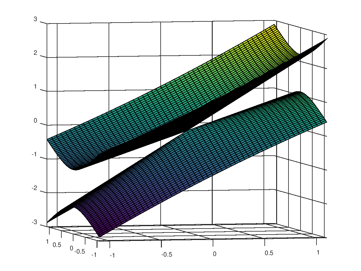
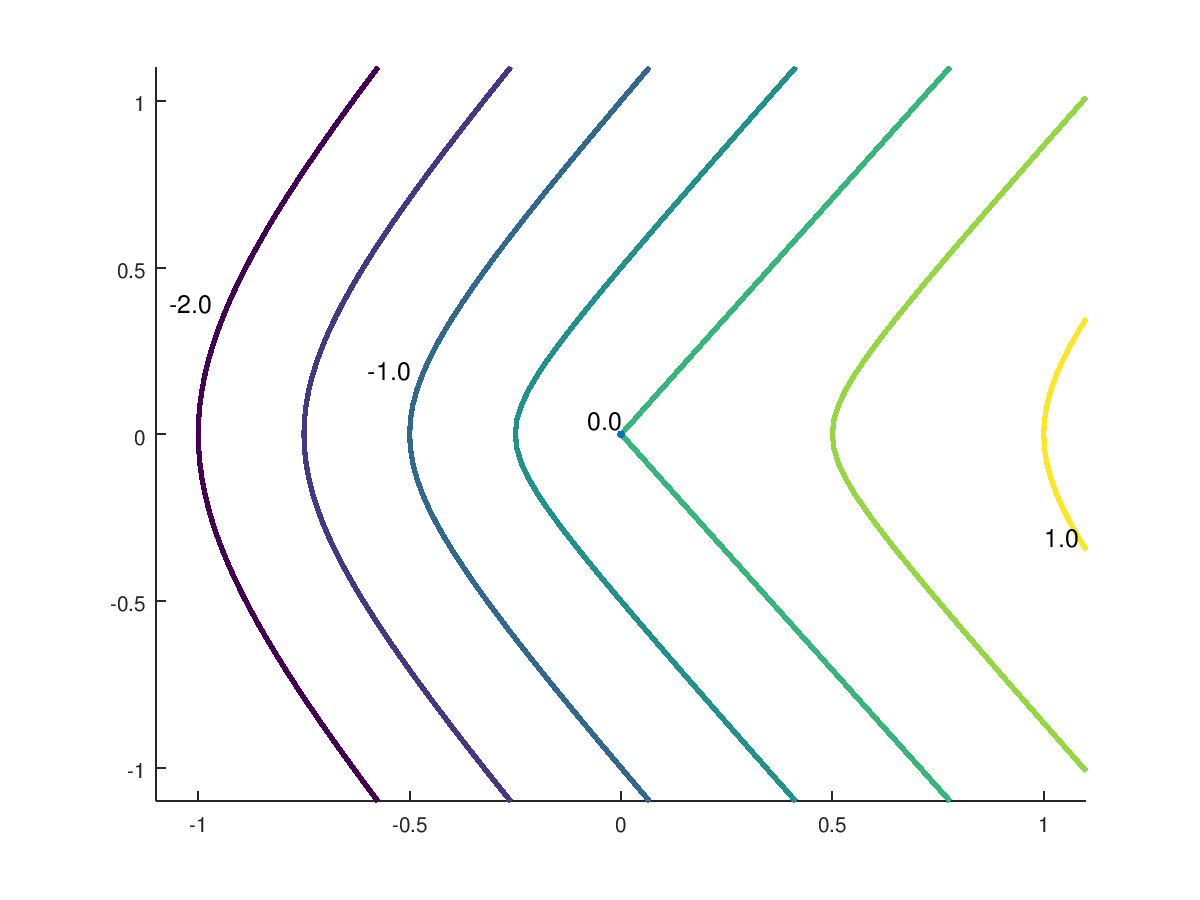
where is the sign definite matrix that spans the orthogonal complement to the differential . Since for any , the set of points of where can be locally represented as a function of is clopen in the subspace topology of . We conclude that can be represented by a function of globally, i.e. as long as the closure of in does not hit the boundary of . In a slight abuse of notation, we will refer to this function as . Figure 3(left) shows examples of the curves for the family from equation (1.6) and two different initial points .
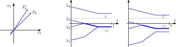
The matrices on the curve have fixed eigenspaces but their eigenvalues change with . For small positive the eigenvalues and above decrease with the constant speed while the eigenvalues below increase because the derivative in (4.17) is positive. This closes the gap below the eigenvalue and decreases the spectral radius (operator norm) of . Therefore, the curve will intersect the egress set (4.14) at some time before it reaches the boundary .
Setting and , we determine such that and repeat the process starting at . We then join the pieces together,
| (4.18) |
There are two ways in which we will terminate this recursive process. If an egress point is reached (which has no eigenvalues strictly smaller than and equation (4.17) becomes undefined due to ), we continue as a constant, for . An example of this is shown in Figure 3(middle). The case which we previously excluded can now be absorbed into this rule.
Alternatively, since decreases from an initial value below at the constant rate , we will reach a point in at some . In this case we also continue as a constant for , see Figure 3(right) for an example (with in this particular case). The case can now be absorbed into the above description by setting .
The preceding paragraphs show that the final values belong to the set , see equation (4.11), and that acts as identity on for all . This suggest that we have a deformation retraction
| (4.19) |
if we establish that the trajectories define a continuous mapping .
We first note that each trajectory is continuous in by construction. Therefore, we need to show that starting at a point which is near will result in being near . A perturbation of arbitrarily small norm may split multiple eigenvalues, therefore if with , then, in general, with (in fact, generically, ). However,
with some universal101010The constant is independent of but may depend on the norm used for ; in case of the operator norm, Weyl inequality yields . constant , and therefore after a time of order , the -th eigenvalue will collide with -th eigenvalue. To put it more precisely, there is , , such that . By choosing to be sufficiently small (while is small but fixed), we ensure that is still in . By noting that the trajectories are continuous in uniformly with respect to , we conclude that is close to .
For two initial points and in the same set , the curves and will remain nearby for any bounded time . This can be seen, for example, as stability of the transversal intersection of the manifold and the manifold (4.16). The stability is with respect to the parameters , and and the spectral projections are continuous in precisely because belongs the same set .
We now chain the two argument in the alternating fashion: short time to bring two points to the same set , long time along smooth trajectories until one of the trajectories reaches an egress point, then short time to bring them to the same set and so on. Since we iterate a bounded number of times, the composition is a continuous mapping. ∎
Given a topological space denote by the cone of (here ), by the suspension of , and by the reduced suspension of , where . Note that if is a CW-complex, then is homotopy equivalent to . In Lemma 4.4 we saw that is homotopy equivalent to the union of and the space which we aim to understand further. We will now show that is a cone of
| (4.20) |
Lemma 4.6.
Let , and be as in Lemma 4.4. Then, for sufficiently small , the topological space is homeomorphic to and the topological space
| (4.21) |
is homeomorphic to .
Remark 4.7.
Proof.
The choice of ensured that is a homeomorphism from to
| (4.24) |
We will now describe the homeomorphism from to .
Given a point , consider the intersection of with the plane
| (4.25) |
Mimicking the proof of Lemma 4.4, we conclude that the intersection is a 1-dimensional submanifold which has a connected component containing the matrix . Moreover, implicit differentiation at yields
| (4.26) |
therefore the submanifold can be represented by a function of ,
| (4.27) |
When , we also have because equation (4.26) implies . We remark that is bounded away from zero uniformly in and , therefore, when is sufficiently small, will remain in until . Thus the function is a well-defined111111Namely, for all . mapping from to . It is evidently continuous.
The properties of imply that contains no multiples of identity and no positive semidefinite matrices except for the zero matrix. Therefore, for every , ,
| (4.28) |
is well-defined, and we also have . Thus
| (4.29) |
is a well-defined continuous mapping from to . It remains to verify that is the inverse of . It is immediate that . To prove that we observe that the intersection , corresponding to of equation (4.28), contains ; we only need to show that and belong to the same connected component of .
The point on the plane (4.25) corresponds to and some . Decreasing from this point decreases and therefore decreases the operator norm of . Thus we will not hit the boundary of as long as . Therefore, we will arrive to the matrix while staying on the same connected component.
We have established the first part of the lemma. To understand the quotient in (4.21), we note that
completing the proof. ∎
Given a vector bundle denote by the symmetric tensor product of . Namely, is the vector bundle over the same base as ; the fiber of over a point is equal to the symmetric tensor product with itself of the fiber of over the same point. Choosing a Euclidean metric on we can identify with the bundle whose fiber over a point is the space of all self-adjoint isomorphisms of the fiber of over the same point. Then by we denote the bundle of traceless elements of . Obviously
| (4.30) |
where is the trivial rank 1 bundle over the base of . Finally, let be the tautological bundle over the Grassmannian : the fiber of this bundle over is the vector space itself.
Lemma 4.8.
Recall the relative index of the eigenvalue, equation (1.13), which in the present situation is equal to . Then the space with is homotopy equivalent to the Thom space of the real vector bundle over the Grassmannian ,
| (4.31) |
The rank of the bundle is , where is given by (1.11). The bundle is non-orientable if and is even, and orientable otherwise.
Remark 4.9.
Let us consider the boundary case or, equivalently, . The Grassmannian is a single point, so the vector bundle is simply a real vector space of dimension . Its Thom space is the one-point compactification of , namely the sphere . Correspondingly, the cone is homotopy equivalent to the ball .
In combination with Remark 4.7 we get that the normal data at the bottom eigenvalue is homotopy equivalent to the pair
| (4.32) |
Proof.
The homotopy equivalence has been established in [A11, Theorem 1] and the proof thereof. For completeness we review the main steps here.
Fixing an arbitrary unit vector we define
| (4.33) |
One can show that is contractible: if is the projection onto , consider
| (4.34) |
where acts on the eigenvalues of as
| (4.35) |
followed by a normalization to get unit trace. Using interlacing inequalities121212A particularly convenient form for this task can be found in [BKKM19, Thm 4.3]. for the rank one perturbation (up to rescaling) of by , one can show that (4.34) is a well-defined retraction. In particular, (4.35) does not produce a zero matrix (which cannot be trace-normalized) and the result of (4.34) is not in for any .
We now obtain that is homotopy equivalent to the Thom space of the normal bundle of in . Indeed, a tubular neighborhood of in is diffeomorphic to the normal bundle of , while the above retraction allows one to show is homotopy equivalent to .
The normal bundle of in is a Whitney sum of the normal bundle of in
| (4.36) |
and the normal bundle of in . The fiber in the former bundle is : it consists of the directions in which can rotate out of . Therefore the former bundle is . The fiber in the normal bundle of in consists of all self-adjoint perturbations to the operator that preserve its kernel and unit trace. Identifying these with the space of traceless self-adjoint operators on , we get . We get (4.31) after recalling that .
To calculate the rank we use
| (4.37) |
and
| (4.38) |
giving in total in the real case and in the complex case.
Recall that a real vector bundle is orientable if and only if its first Stiefel–Whitney class vanishes (here is the base of the bundle). The first Stiefel–Whitney class is additive with respect to the Whitney sum, therefore
| (4.39) |
Using additivity on equation (4.30) gives because is zero for the trivial bundle. The classical formulas for the Stiefel–Whitney classes of symmetric tensor power (see, for example, [FF16, Sec. 19.5.C, Theorem 3]) yield and, finally,
| (4.40) |
Since the real tautological bundle is not orientable and has rank , vanishes if and only if is zero modulo 2, completing the proof of the lemma. ∎
Proof of Theorem 4.1.
We review how the preceding lemmas link together to give the proof of the theorem. Lemma 4.3 shows that the smooth part gives the classical contribution to the sublevel set quotient and we can focus on understanding the transversal part . We remark that by Corollary 3.5 the point remains non-degenerate topologically critical when we replace with .
Recall [H94b, Cor. 16.1.6] that the reduced suspension of a Thom space of a vector bundle is homeomorphic to the Thom space of the Whitney sum of this bundle with the trivial rank 1 bundle , i.e.
| (4.42) |
The bundle is orientable if and only if is orientable; its rank is one plus the rank of . Lemma 4.8 supplies both pieces of information and completes the proof of the theorem. ∎
5. Proofs of Theorem 1.17 and Theorem 1.10
Proof of Theorem 1.17, part (1).
As established in Theorem 4.1, the bundle is orientable if or if and is odd, and we can use the homological version of the Thom isomorphism theorem [MS74, Lemma 18.2], which gives
| (5.1) |
which is the right-hand side of (1.15) in the corresponding cases.
Remark 5.1.
Both formulas (5.1) and (5.2) are very particular cases of [S03, Theorem 3.10]. We summarize this theorem here at a level of generality which is still incomplete but sufficient for our needs. Recall that the orientation character on a path-connected manifold with the fundamental group is the map that sends a loop to 1 if the orientation is preserved along and to if it is reversed along . In fact, can be viewed as the first Stiefel–Whitney class with values in the multiplicative instead of the additive one. Multiplication by defines a representation of the group on and, consequently, endows with the structure of a -module, which will be denoted by . As -modules, if is orientable and if is nonorientable. Theorem 3.10 of [S03] states that given a vector bundle of rank and a -module , the -th homology of with closed support (also known as Borel-Moore homology, [BM60]) and local coefficients in is equal to -th homology of with closed support and local coefficients in . Formulas (5.1) and (5.2) correspond to the case . Note that the Borel-Moore homologies of are equal to the reduced homologies of its one-point compactification ([G98, item (1) on p. 130]) which in our case is the Thom space of as the base space is compact.
We remark that in the original formulation of [S03, Theorem 3.10], an orientation sheaf is used instead of the -module , but these two objects are in fact the same under the canonical identification of the set of locally constant sheaves over with values in an abelian group and the set of -modules on [S09, Theorem 2.5.15].
Remark 5.2.
Part (2) of Theorem 1.17 will be obtained as a combination of the next two lemmas. Lemma 5.3 provides an expression for the Poincaré polynomial of twisted homologies by relating it to the Poincaré polynomial of the oriented Grassmannian . Lemma 5.4 below collates known expressions for the Poincaré polynomials of Grassmannians and oriented Grassmannians.
Lemma 5.3.
In the setting of Theorem 1.17, the Poincaré polynomials of the relative homology groups is equal to
| (5.4) |
where denotes the Poincaré polynomial of the manifold .
Proof.
Since we already established part (1) of Theorem 1.17, we only need to show that the Poincaré polynomial of the homology groups is equal to .
We will use homologies with coefficients in (or ). Indeed, since the Betti numbers ignore the torsion part of , the Universal Coefficients Theorem (see, e.g. [H02, Sec. 3.A]) implies they can be calculated as the rank of with any torsion-free abelian group . The benefit of using is that now any chain in can be uniquely represented as a sum of a symmetric and a skew-symmetric chains with coefficients in ,
| (5.5) |
where is the orientation reversing involution of (viewed as a double cover of ). The analogous statement is of course wrong in integer coefficients, as .
Since the boundary operator preserves the parity of a chain, the homology decomposes into the direct sum of homologies of -symmetric and -skew-symmetric chains on . The former homology coincides with the usual homology of . The latter yields, by definition, the twisted -homology of . To summarize, we obtain
| (5.6) |
The sum in (5.6) translates into the sum of Poincaré polynomials, yielding the middle line in (5.4). ∎
Lemma 5.4.
Let , . The Poincaré polynomials of the Grassmannians , and are given by
| (5.7) | ||||
| (5.8) | ||||
| (5.9) |
Remark 5.5.
Proof.
Betti numbers for complex Grassmannians were established by Ehresmann, see [E34, Theorem on p. 409, section II.7]. The -the Betti number is zero if is odd and is equal to the number of Young diagrams with cells that fit inside the rectangle, if is even. The Poincaré polynomial is nothing but the generating function for this restricted partition problem. The latter is well known to be of the form (5.7), see [A76, Theorem 3.1, p. 33].
The -th Betti number of the real Grassmannian has a similar combinatorial description [I49, Theorem IV, p. 108]: it is equal to the number of Young diagrams of cells that fit inside the rectangle and have even length differences for each pair of columns and for each pair of rows. From this it can be shown that the Poincaré polynomial satisfies (5.8) (see also [CK13, Theorem 5.1]). We remark that for and both even, (5.8) is a consequence of (5.7) because the corresponding Young diagrams must be made up from squares.
Finally, the oriented Grassmannian is a homogeneous space, namely
| (5.10) |
The corresponding Poincaré polynomial has been computed within the general theory of de Rham cohomologies of homogeneous spaces, see, for example, [GHV76, Chap. XI]. Up to notation, the first line of (5.9) corresponds to [GHV76, Lines 2-3, col. 3 of Table II on p. 494], the second line of (5.9) corresponds to [GHV76, Lines 2-3, col. 1 of Table III on p. 496] and the third line of (5.9) corresponds to [GHV76, Lines 2-3, col. 2 of Table III on p. 495]. ∎
Remark 5.6.
In fact, in the second line of (1.16) can be explained from the theory of characteristic classes of real vector bundles: if and are infinite Grassmannian and oriented Grassmann of planes, respectively, i.e. the direct limits and as , then the ring of the de Rham cohomologies of is generated by the Pontryagin classes of the corresponding tautological bundle, while the ring of the de Rham cohomologies of is generated by the Pontryagin classes of the corresponding tautological bundle, if is odd, and by the Pontryagin classes and the Euler class of the corresponding tautological bundle, of is even. So, for with even the de Rham cohomologies of and coincide, implying the second line of (1.16).
The Poincaré polynomials in part (2) of Theorem 1.17 specify the free part of the homology groups . Namely they are the generating functions of the number of copies of in said homologies. In fact, we can completely specify these homologies by also describing their torsion part. This is done in Lemma 5.7 below which is also instrumental in proving Theorem 1.10.
Lemma 5.7.
Assume that . In the setting of Theorem 1.17, the torsion part of the relative homology group is equal to copies of , where depends on , and . The generating function of is given by
| (5.11) |
In Table 2 we give the generating functions (5.11) for a range of multiplicities and under the assumption that .
| 0 | 0 | |||||||
| 0 | 0 | |||||||
| 0 | 0 | |||||||
| 0 | 0 | |||||||
| 0 | 0 | |||||||
| 0 | 0 | |||||||
| 0 | ||||||||
Proof of Lemma 5.7.
It is well known [E37, P50] that all nontrivial elements of finite order in the -homology groups of real Grassmannians have order , i.e. the torsion part of any -homology group consists of several copies of . For any such manifold , denote this number of copies by . Define the generating function of the torsion part of by
| (5.12) |
Let be the Poincaré polynomial of -homologies of . As observed in [H17a, Lemma 3.2], the Universal Coefficient Theorem (see, e.g. [H02, Sec. 3.A]) implies
| (5.13) |
The Poincaré polynomial of -homologies of the Grassmannian is well known to be
| (5.14) |
Combining (5.14) with the first line of (1.16) results in the first line of (5.11).
Furthermore, if the fundamental group of is equal to , then the twisted analog of formula (5.13) holds: we just need to replace each generating function , and by its analogue for twisted homologies. When the coefficients are , there is no difference between symmetric and skew-symmetric chains, therefore . To summarize, the twisted analogue of (5.13) becomes
| (5.15) |
In the relevant cases, is given by the second and third line of (1.16). Substituting them, together with (5.14), into (5.15) yields the second and third line of (5.11) correspondingly. ∎
Proof of Theorem 1.10.
To show that a non-degenerate topologically critical point (in the sense of Definition 1.14) is not regular in the sense of Definition 1.1, we use Theorem 1.17 which has been proved already and demonstrate that the homologies on the right-hand side of (1.15) are non-trivial. In all case except , even and odd , (1.16) shows that the free part of the corresponding homologies is not trivial. When , is even and is odd, the free part is trivial, but the torsion part is non-trivial by Lemma 5.7. ∎
Proof of Corollary 1.18.
A critical point is a point of local maximum if an only if the local Morse data is homotopy equivalent to .
If is a maximum, its contribution to the Poincare polynomial is equal to , which occurs only in the cases described by Corollary 1.18.
To establish sufficiency, we compute the local Morse data at . If condition (1) is satisfied, the normal data at the point has been computed in Remark 4.9, . From condition (2) we get the tangential data
| (5.16) |
By [GM88, Thm I.3.7], the local Morse data is then
| (5.17) |
implying the point is a maximum.
Similarly, a critical point is a point of local minimum if an only if the local Morse data is homotopy equivalent to . If is a minimum, its contribution to the Poincare polynomial is equal to , which occurs only in the cases described by Corollary 1.18.
Appendix A Hellmann–Feynman Theorem
In this section we review the mathematical formulation of the formula that is known in physics as Hellmann–Feynman Theorem or first-order perturbation theory. We base our formulation on [K95, Thm II.5.4] (see also [G09]).
Theorem A.1.
Let be differentiable at . Let be an eigenvalue of of multiplicity , be its eigenspace, and be a linear isometry satisfying . Then, for small enough , there are exactly eigenvalues of close to and they are given by
| (A.1) |
where are the eigenvalues of the matrix .
Appendix B Twisted Thom space homologies from Poincaré–Lefschetz duality
The Poincaré–Lefschetz duality (see, e.g. [H02, Theorem 3.43]) states that if is compact orientable -dimensional manifold with boundary , then
| (B.1) |
There is also a twisted analogue141414See [G08, Prop 15.2.10] or [DK01, chapter 5]. It is also sometimes known as Poincaré–Verdier duality, see [I86, VI.3]. of Poincaré–Lefschetz duality for non-oriented manifolds: if is compact non-orientable -dimensional manifold with boundary , then
| (B.2) |
Here, the twisted homology was already introduced prior to the formulation of Theorem 1.17. To define twisted cohomology groups, denote by the orientation cover of and by the corresponding orientation-reversing involution. are the cohomologies of the cochain complex defined on the spaces of cochains satisfying for every chain in (see [H02, Se. 3H] for a more general point of view). Such cochains will be called skew-symmetric cochains. Note that the space of skew-symmetric cochains can be identified with the dual space to the space of skew-symmetric chains, as expected.
(a) Assume now that is even. Then the base of the vector bundle is non-orientable and, since the vector bundle is also non-orientable, the total space is orientable. By the usual Poincaré–Lefschetz duality (B.1),
| (B.3) |
where is the dimension of the total space . In the last identification we used that the base is the deformation retract of the total space of the bundle.
Further, since is non-orientable when is even, we use the twisted analog of Poincaré duality for nonorientable manifolds (see [H02, Theorem 3H.6] as well as (B.2) with ) to get
| (B.4) |
where we used
| (B.5) |
(b) Consider the case of odd . Then the base is orientable, the bundle is non-orientable and therefore the total space is non-orientable. By the twisted Poincaré-Lefschetz duality (B.2),
| (B.6) |
The orientation double cover of can be constructed from the tautological bundle of the oriented Grassmannian in the same way as was constructed from the tautological bundle of the Grassmannian by relations (4.31) and (4.42). In particular, is a bundle of rank over the oriented Grassmannian . Therefore, retracting the unit ball bundle of to its base, we get that the integer cohomology groups of are isomorphic to the integer cohomology groups of the oriented Grassmannian , i.e.
Moreover, the retraction can be made to preserve the spaces of skew-symmetric chains, which implies that
| (B.7) |
When is odd, is orientable and so is . Moreover, the map from the usual Poincare duality (see [H02, Thm. 3.30] as well as (B.1) with ) applied to sends the equivalence classes of skew-symmetric cochains to the corresponding skew-symmetric chains. Thus, we arrive to
| (B.8) |
To summarize, we get the corresponding line in (1.15) whether is even or odd.
References
- [A72] V. I. Arnold, Modes and quasimodes, Funkcional. Anal. i Priložen. 6 (1972), 12–20, English translation: Funct. Anal. Appl., 6:2 (1972), 94–101.
- [A76] G. E. Andrews, The theory of partitions, Encyclopedia of Mathematics and its Applications, Vol. 2, Addison-Wesley Publishing Co., Reading, Mass.-London-Amsterdam, 1976.
- [A11] A. A. Agrachev, Spaces of symmetric operators with multiple ground states, Funktsional. Anal. i Prilozhen. 45 (2011), 1–15, translation in Funct. Anal. Appl. 45 (2011), no. 4, 241–251.
- [AG22] L. Alon and M. Goresky, Morse theory for discrete magnetic operators and nodal count distribution for graphs, preprint arXiv:2212.00830, 2022.
- [AGZV12] V. I. Arnold, S. M. Gusein-Zade, and A. N. Varchenko, Singularities of differentiable maps. Volume 1, Modern Birkhäuser Classics, Birkhäuser/Springer, New York, 2012, Classification of critical points, caustics and wave fronts, Reprint of the 1985 edition.
- [APS97] A. A. Agrachev, D. Pallaschke, and S. Scholtes, On Morse theory for piecewise smooth functions, J. Dynam. Control Systems 3 (1997), 449–469.
- [B79] M. D. Bronšteĭn, Smoothness of roots of polynomials depending on parameters, Sibirsk. Mat. Zh. 20 (1979), 493–501, 690, English translation: Siberian Math. J. 20 (1979), no. 3, 347–352 (1980).
- [B13] G. Berkolaiko, Nodal count of graph eigenfunctions via magnetic perturbation, Anal. PDE 6 (2013), 1213–1233, preprint arXiv:1110.5373.
- [BBRS12] R. Band, G. Berkolaiko, H. Raz, and U. Smilansky, The number of nodal domains on quantum graphs as a stability index of graph partitions, Comm. Math. Phys. 311 (2012), 815–838.
- [BC18] G. Berkolaiko and A. Comech, Symmetry and Dirac points in graphene spectrum, J. Spectr. Theory 8 (2018), 1099–1147, preprint arXiv:1412.8096.
- [BCR98] J. Bochnak, M. Coste, and M.-F. Roy, Real algebraic geometry, Ergebnisse der Mathematik und ihrer Grenzgebiete (3) [Results in Mathematics and Related Areas (3)], vol. 36, Springer-Verlag, Berlin, 1998, Translated from the 1987 French original, Revised by the authors.
- [BH04] A. Banyaga and D. Hurtubise, Lectures on Morse homology, Kluwer Texts in the Mathematical Sciences, vol. 29, Kluwer Academic Publishers Group, Dordrecht, 2004.
- [BKKM19] G. Berkolaiko, J. B. Kennedy, P. Kurasov, and D. Mugnolo, Surgery principles for the spectral analysis of quantum graphs, Trans. Amer. Math. Soc. 372 (2019), 5153–5197.
- [BM60] A. Borel and J. C. Moore, Homology theory for locally compact spaces, Michigan Math. J. 7 (1960), 137–159.
- [BV04] S. Boyd and L. Vandenberghe, Convex optimization, Cambridge University Press, Cambridge, 2004.
- [C51] S.-S. Chern, Topics in differential geometry, The Institute for Advanced Study, Princeton, N. J., 1951.
- [C90] F. H. Clarke, Optimization and nonsmooth analysis, second ed., Classics in Applied Mathematics, vol. 5, Society for Industrial and Applied Mathematics (SIAM), Philadelphia, PA, 1990.
- [C94] S. J. Cox, Extremal eigenvalue problems for the Laplacian, Recent advances in partial differential equations (El Escorial, 1992), RAM Res. Appl. Math., vol. 30, Masson, Paris, 1994, pp. 37–53.
- [CdV13] Y. Colin de Verdière, Magnetic interpretation of the nodal defect on graphs, Anal. PDE 6 (2013), 1235–1242, preprint arXiv:1201.1110.
- [CK13] L. Casian and Y. Kodama, On the cohomology of real grassmann manifolds, arXiv:1309.5520 [math.AG] (2013), 13 pages.
- [CNGP+09] A. Castro Neto, F. Guinea, N. Peres, K. Novoselov, and A. Geim, The electronic properties of graphene, Rev. Mod. Phys. 81 (2009), 109–162.
- [D80] A. Dold, Lectures on algebraic topology, second ed., Grundlehren der Mathematischen Wissenschaften [Fundamental Principles of Mathematical Sciences], vol. 200, Springer-Verlag, Berlin-New York, 1980.
- [D01] D. Duffie, Dynamic asset pricing theory, 3rd ed., Princeton University Press, Princeton, NJ, 2001.
- [DK01] J. F. Davis and P. Kirk, Lecture notes in algebraic topology, Graduate Studies in Mathematics, vol. 35, American Mathematical Society, Providence, RI, 2001.
- [DYK04] W. Domcke, D. R. Yarkony, and H. Köppel, Conical intersections: Electronic structure, dynamics and spectroscopy, World Scientific, 2004.
- [E34] C. Ehresmann, Sur la topologie de certains espaces homogènes, Ann. of Math. (2) 35 (1934), 396–443.
- [E37] C. Ehresmann, Sur la topologie de certaines variétés algébriques réelles, J. Math. Pures Appl. (9) 16 (1937), 69–100 (French).
- [ELS21] M. J. Esteban, M. Lewin, and E. Séré, Dirac–Coulomb operators with general charge distribution II. The lowest eigenvalue, Proc. London Math. Soc. 123 (2021), 345–383.
- [F65] E. A. Feldman, The geometry of immersions. I, Trans. Amer. Math. Soc. 120 (1965), 185–224.
- [FF89] A. Fomenko and D. Fuks, A course in homotopical topology, Nauka, Moscow, 1989, in Russian; English translation does not have the relevant appendix.
- [FF16] A. Fomenko and D. Fuchs, Homotopical topology, second ed., Graduate Texts in Mathematics, vol. 273, Springer, Cham, 2016.
- [FK18] N. Filonov and I. Kachkovskiy, On the structure of band edges of 2-dimensional periodic elliptic operators, Acta Math. 221 (2018), 59–80.
- [FW12] C. L. Fefferman and M. I. Weinstein, Honeycomb lattice potentials and Dirac points, J. Amer. Math. Soc. 25 (2012), 1169–1220.
- [G98] V. Ginzburg, Geometric methods in the representation theory of Hecke algebras and quantum groups, Representation theories and algebraic geometry (Montreal, PQ, 1997), NATO Adv. Sci. Inst. Ser. C: Math. Phys. Sci., vol. 514, Kluwer Acad. Publ., Dordrecht, 1998, Notes by Vladimir Baranovsky, pp. 127–183.
- [G08] R. Geoghegan, Topological methods in group theory, Graduate Texts in Mathematics, vol. 243, Springer, New York, 2008.
- [G09] V. Grushin, Multiparameter perturbation theory of Fredholm operators applied to Bloch functions, Math. Notes 86 (2009), 767–774.
- [GHV76] W. Greub, S. Halperin, and R. Vanstone, Connections, curvature, and cohomology, Pure and Applied Mathematics, Vol. 47-III, Academic Press [Harcourt Brace Jovanovich, Publishers], New York-London, 1976, Volume III: Cohomology of principal bundles and homogeneous spaces.
- [GM88] M. Goresky and R. MacPherson, Stratified Morse theory, Results in Mathematics and Related Areas (3), vol. 14, Springer-Verlag, Berlin, 1988.
- [H94a] M. W. Hirsch, Differential topology, Graduate Texts in Mathematics, vol. 33, Springer-Verlag, New York, 1994, Corrected reprint of the 1976 original.
- [H94b] D. Husemoller, Fibre bundles, third ed., Graduate Texts in Mathematics, vol. 20, Springer-Verlag, New York, 1994.
- [H02] A. Hatcher, Algebraic topology, Cambridge University Press, Cambridge, 2002.
- [H06] A. Henrot, Extremum problems for eigenvalues of elliptic operators, Frontiers in Mathematics, Birkhäuser Verlag, Basel, 2006.
- [H17a] C. He, Torsions of integral homology and cohomology of real grassmannians, arXiv:1709.05623 [math.AT] (2017), 6 pages.
- [H17b] A. Henrot (ed.), Shape optimization and spectral theory, De Gruyter Open, Warsaw, 2017.
- [HHO13] B. Helffer and T. Hoffmann-Ostenhof, On a magnetic characterization of spectral minimal partitions, J. Eur. Math. Soc. (JEMS) 15 (2013), 2081–2092.
- [HUL99] J.-B. Hiriart-Urruty and A. S. Lewis, The Clarke and Michel-Penot subdifferentials of the eigenvalues of a symmetric matrix, Comput. Optim. Appl. 13 (1999), 13–23.
- [I49] H. Iwamoto, On integral invariants and Betti numbers of symmetric Riemannian manifolds. I, J. Math. Soc. Japan 1 (1949), 91–110.
- [I86] B. Iversen, Cohomology of sheaves, Universitext, Springer-Verlag, Berlin, 1986.
- [K95] T. Kato, Perturbation theory for linear operators, Classics in Mathematics, Springer-Verlag, Berlin, 1995, Reprint of the 1980 edition.
- [K16] P. Kuchment, An overview of periodic elliptic operators, Bull. Amer. Math. Soc. (N.S.) 53 (2016), 343–414.
- [M47] E. W. Montroll, Dynamics of a square lattice .1. frequency spectrum, J. Chem. Phys. 15 (1947), 575–591.
- [M63] J. Milnor, Morse theory, Based on lecture notes by M. Spivak and R. Wells. Annals of Mathematics Studies, No. 51, Princeton University Press, Princeton, N.J., 1963.
- [M93] B. Mishra, Algorithmic algebra, Texts and Monographs in Computer Science, Springer-Verlag, New York, 1993.
- [M21] S. Matsika, Electronic structure methods for the description of nonadiabatic effects and conical intersections, Chemical Reviews 121 (2021), 9407–9449.
- [MP99] D. Motreanu and P. D. Panagiotopoulos, Minimax theorems and qualitative properties of the solutions of hemivariational inequalities, Nonconvex Optimization and its Applications, vol. 29, Kluwer Academic Publishers, Dordrecht, 1999.
- [MS74] J. W. Milnor and J. D. Stasheff, Characteristic classes, Annals of Mathematics Studies, No. 76, Princeton University Press, Princeton, N. J.; University of Tokyo Press, Tokyo, 1974.
- [NB11] L. Narici and E. Beckenstein, Topological vector spaces, second ed., Pure and Applied Mathematics, vol. 296, CRC Press, Boca Raton, FL, 2011.
- [P50] L. S. Pontryagin, Characteristic cycles on differentiable manifolds, Amer. Math. Soc. Translation 1950 (1950), 72.
- [P22] H. Price, Simulating four-dimensional physics in the laboratory, Physics Today 75 (2022), 38–44.
- [R80] J. B. Rudjak, On the Thom-Dold isomorphism for nonorientable vector bundles, Dokl. Akad. Nauk SSSR 255 (1980), 1323–1325.
- [S52] M. Smollett, The frequency spectrum of a 2-dimensional ionic lattice, Proc. Phys. Soc. (London) A 65 (1952), 109–115.
- [S03] E. G. Sklyarenko, The Thom isomorphism for nonorientable bundles, Fundam. Prikl. Mat. 9 (2003), 55–103, Russian; translation in J. Math. Sci. (N.Y.) 136 (2006), no. 5, 4166–4200.
- [S09] T. Szamuely, Galois groups and fundamental groups, Cambridge Studies in Advanced Mathematics, vol. 117, Cambridge University Press, Cambridge, 2009.
- [T79] D. J. A. Trotman, Stability of transversality to a stratification implies Whitney -regularity, Invent. Math. 50 (1978/79), 273–277.
- [V09] C. Valero, Morse theory for eigenvalue functions of symmetric tensors, J. Topol. Anal. 1 (2009), 417–429.
- [VH53] L. Van Hove, The occurence of singularities in the elastic frequency distribution of a crystal, Phys. Rev. 89 (1953), 1189–1193.
- [vNW29] J. von Neuman and E. Wigner, Über merkwürdige diskrete Eigenwerte. Über das Verhalten von Eigenwerten bei adiabatischen Prozessen, Physikalische Zeitschrift 30 (1929), 467–470.
- [W65] H. Whitney, Tangents to an analytic variety, Ann. of Math. (2) 81 (1965), 496–549.