Appendix and Online Material

We present the experiment details in this part of the paper. When unspecificed, the embedding dimension is given by $d=32$.

Appendix A Model configurations

In our experiments, we main employ the Item2vec model [barkan2016item2vec], the BERT model [devlin2018bert], and the two-tower Dense-layer-based, GRU-based, and self-attention-based recommendation models.

  • [leftmargin=*]

  • β€’

    Item2vec: the model is a direct adaptation of the renown NLP Word2vec model [mikolov2013distributed], by replacing the original word sequence by user behavior sequence. Therefore, the algorithm takes the window size and #negative samples as hyper-parameters, which we vary between {2,3}23\{2,3\} and {2,3,4}234\{2,3,4\}, respectively, to generate pre-trained embeddings whose performances will cover a wide spectrum of the metrics we consider (showed in Figure LABEL:fig:OOD-clf and LABEL:fig:OOD-reco).

  • β€’

    BERT: since the sentence and descriptions for the items are relatively short, we use the ALBERT model (a simplified version of BERT) whose pre-trained version is publicly available, together with the dedicated NLP preprocessing pipeline for fine-tuning 111https://www.tensorflow.org/official_models/fine_tuning_bert. During the fine-tuning, we only re-train the last layer of ALBERT, which is equivalent to applying a logistic regression using second-to-last hidden layer’s output as input features We refer to this linear-head-tuning setting as BERT-LR.

  • β€’

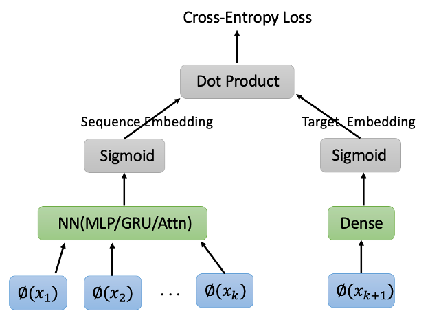
    Two-tower recommendation models: the architecture of the model is presented in Figure LABEL:fig:online_evala, where we use the Dense layer, GRU layer, and self-attention layer to aggregate the users’ previous interaction sequence. Since our experiments are mostly illustrational, we fix the hidden dimensions of all the Dense layers as {32,16}, the hidden dimension of the GRU and self-attention layer as 32, instead of tuning them exhaustively.

The model variations that we created include: CL-LR, CL-IP, BERT-LR, BERT-IP. In particular, CL-LR means we use the CL-trained embeddings as features for the downstream logistic regression model, CL-IP means we use the pre-trained embeddings to compute the kernel $K_{\phi}$, and use $K_{\phi}$ for a standard kernel SVM model. As for BERT-IP, we simply extract the second-to-last layer’s hidden representation as pre-trained embedding, and follow the same procedure as CL-IP.

We mention that for the illustrational experiments in Section 3, we use $d=16$ for the sake of visualization. For each dataset, we train the Item2vec model as described above, using: window size=3 and #negative sample=3. We then randomly pick one item embedding from each dataset, and show its values from the ten independent runs.

A.1 Training, validation and evaluation

We describe the training, validation, and evaluation procedures for our experiments.

Training. We use off-the-shelf Tensorflow implementation for the Item2vec model and the sequential recommendation models. The code are available in the online materialLABEL:footnote1. We use the base version of the pre-trained ALBERT model 222https://github.com/google-research/albert and its official NLP preprocessing pipeline to obtain the BERT-based embeddings, which are also implemented in Tensorflow. For the CL-based pre-training for entity classification, we use the Gensim python library333https://radimrehurek.com/gensim/parsing/preprocessing.html for preprocessing the NLP data. The kernel SVM model and logistic regression for the above-mentioned CL-X downstream models are implemented using the Scikit-Learn 444https://scikit-learn.org/stable/ package. We use the stochastic gradient descent (RMSprop optimizer) for all the deep learning models, with the learning rate set as 0.005, batch size set as 256, and Glorot initilizations when needed. We also use the $\ell_{2}$ regularization on all the model parameters with the regularization parameter set as $1e-6$ with no decaying schedule.

Validation. For the item classification tasks, we perform validation on the 10% left-out samples using the F1 score as metric. For the sequential recommendation tasks, for each sequence, we use the last interaction for testing, the second-to-last for validation, and the rest for training. We use the Recall@10 metric for validation as well.

Evaluation. For the item classification tasks, the evaluation metrics Micro-F1 and Macro-F1 are computed on the 10% testing samples using the Scikit-Learn package. The recommendation algorithms are evaluated on the last interaction, where we rank the true interacted among all the items, and compute the top-10 Recall, overall NDCG and the mean reciprocal rank MRR. We mention that krichene2020sampled has pointed out the potential issue of using sampled metric, so when computing the NDCG, we include all the candidate items to obtain unbiased result.

All the implementation are carried out in Python, and the computations are conducted on a Linux machine with 16 CPU, 64 Gb memory and two 32Gb Nvidia Tesla V100 GPU.

Refer to caption
Figure A.1: The offline evaluations results for comparing the standard offline evaluation (after correcting for the popularity bias) and the proposed kernel-based evaluation. The reported results have been multiplied by 100. While the standard offline evaluation is unable to differentiate the performance of the three candidate pre-trained embeddings, our proposed kernel-based evaluation clearly shows that Emb3>Emb2>Emb1, which matches the result we observed after deploying online (Figure A.3).
Refer to caption
Figure A.2: The two-tower architecture for our sequential recommendation models in this paper.

Appendix B Real-world experiment and Online testing result

The previous results have provided strong evidence to carry the kernel-based evaluation further to online experiments, which we conduct with ’ECOM’ – a major e-commerce platform in the U.S. The production scenario is that on the item page of ’ECOM’, we rank the recall set according to the customers’ most recent ten views. The recall set are fixed during the online experiments, so the role of pre-trained embeddings are strictly for ranking.

The deployed online ranking model also adopts a similar two-tower architecture described in Figure A.2. The difference is that it also processes the non-embedding features such as rating, popularity, and price range, in a similar fashion described in the Deep & Wide model [cheng2016wide]. The production problem is to select the best-performing pre-trained item embeddings obtained from the three candidate pre-training algorithms:

  • [leftmargin=*]

  • β€’

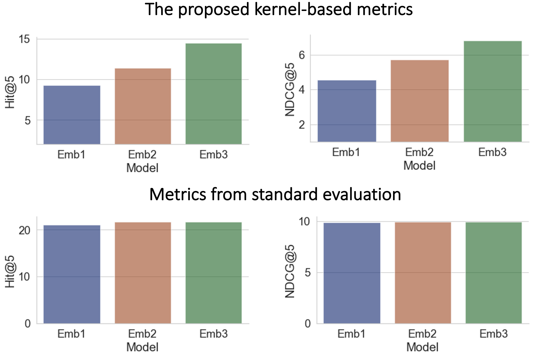
    Emb1: the item embedding trained by Doc2vec [le2014distributed] that uses only the items’ title, brand, and other textual description. This pre-training model is currently in production, so it will serve as the control model in our online experiments.

  • β€’

    Emb2: the complementary item embedding described in the recent work of [xu2020knowledge], which better captures the complementary relationship among items. This approach also includes the contextual features, so it is a generalization of the previous model

  • β€’

    Emb3: the knowledge-graph-based item embedding that is described in [xu2020product]. In general, this approach enhances traditional item embeddings using techniques that generate knowledge graph embeddings.

Refer to caption
Figure A.3: The online A/B/C testing result with Emb1 (Control), Emb2 (Variation 1) and Emb3 (Variation 2), in the dowsntream item-page classification task deployed to ’ECOM’. The orange baselines represent the performance of Emb1, the blue line and bar represent the performance of Emb2, and the green line and bar represent the performance of Emb3.

To carry out the standard offline evaluation, we first plug in each candidate embeddings and retrain the whole downstream Deep&Wide model. Retraining the downstream model is necessary as we discussed earlier. We then compute the offline metrics after correcting for the popularity bias [schnabel2016recommendations], i.e. using popularity to inversely weighting individual samples.

It is obvious that this standard procedure is very inefficient for evaluating pre-trained embeddings – we must retrain and tune each model separately to achieve an overall fair comparison. More importantly, due to the existence of other features, it is hard to justify only by the offline result whether the differences owe entirely to the embeddings’ quality.

In this regard, the proposed kernel-based evaluation can connect the performance more straightforwardly to the pre-trained embeddings, and it enjoys faster computation. The only potential concern is that the kernel-based evaluation may not truly imply the online performance. To resolve this concern, we conduct both offline and online evaluations, and compare the offline evaluation results with the online A/B/C testing outcome. They are provided in Figure LABEL:tab:offline_eval and Figure A.3.

Judging from the kernel-based evaluation in Figure LABEL:tab:offline_eval, we clearly have: Emb3>Emb2>Emb1 in terms of both the recall and NDCG (Table LABEL:tab:offline_eval). On the other hand, the comparisons are almost edge-to-edge in the standard offline evaluation. The three pre-trained embeddings perform almost the same, and the margins are very thin. While we did not expect the kernel-based evaluation to be so advantageous in telling the candidates apart, this result imply another pro of the kernel-based metric:

  • β€’

    they attribute the difference in performances exclusively to the quality of pre-trained embeddings.

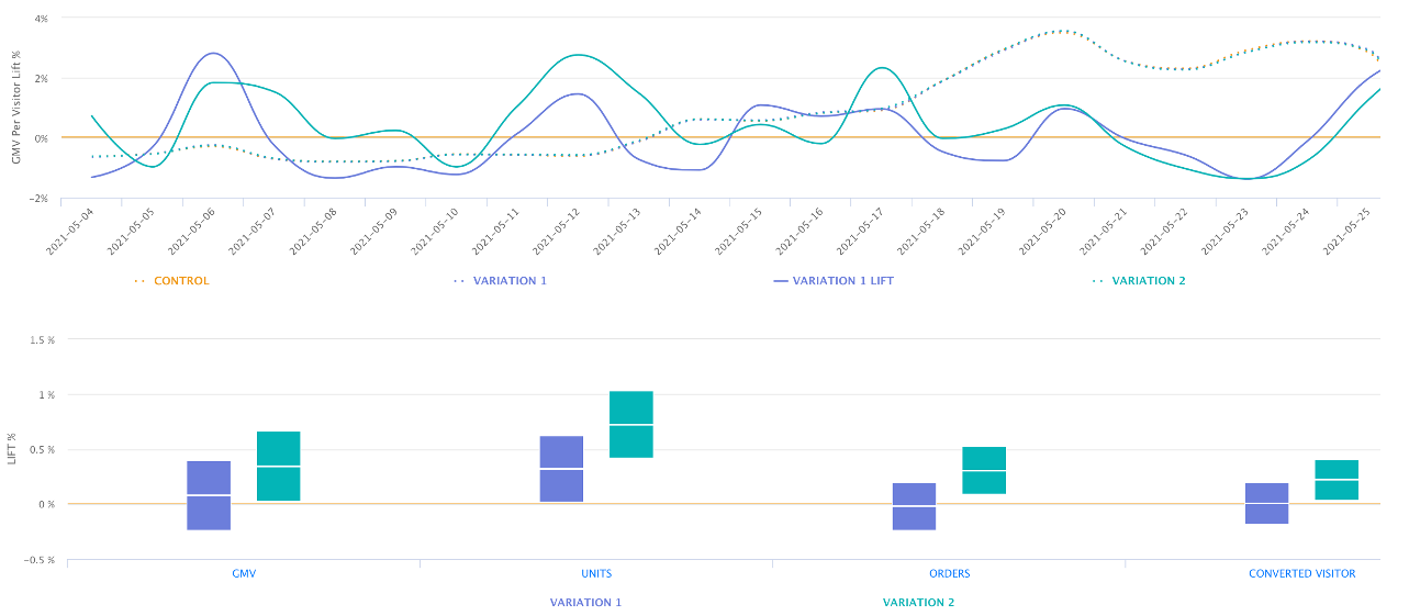
Finally, from the online A/B/C testing result presented in Figure A.3, we indeed observe from real-world performances that Emb3>Emb2>Emb1 in terms of all the revenue-critical metrics – GMV, number of orders, and conversion rate. The deployment result shows that the kernel-based evaluation provides efficient and reliable examinations in terms of how the pre-trained embeddings fits the downstream tasks. Nevertheless, we do point out that the kernel-based evaluation is not meant to replace other offline evaluations. Instead, it adds to the arsenal a convenient and powerful tool for the practitioners to examine and understand pre-trained embeddings.

Appendix C Proofs

We provide the proofs for the propositions and theorem stated in the paper.

C.1 Proof for Proposition 1

Proof.

The proofs for the lower bound often starts by converting the problem to a hypothesis testing task. Denote our parameter space by $\mathcal{B}(k)=\{\beta\in\mathbb{R}^{d}:\|\beta\|_{0}\leq k\}$. The intuition is that suppose the data is generated by: (1). drawing $\beta$ according to an uniform distribution on the parameter space; (2). conditioned on the particular $\beta$, the observed data is drawn. Then the problem is converted to determining according to the data if we can recover the underlying $\beta$ as a canonical hypothesis testing problem.

For any $\delta$-packing $\{\beta_{1},\ldots,\beta_{M}\}$ of $\mathcal{B}(k)$, suppose $B$ is sampled uniformly from the $\delta$-packing, then following a standard argument of the Fano method [wainwright2019high], it holds that:

P(minΞ²^supβ€–Ξ²βˆ—β€–0≀k)βˆ₯Ξ²^βˆ’Ξ²βˆ—βˆ₯2β‰₯Ξ΄/2)β‰₯minΞ²~P(Ξ²~β‰ B),P\big{(}\min_{\hat{\beta}}\sup_{\|\beta^{*}\|_{0}\leq k})\|\hat{\beta}-\beta^{*}\|_{2}\geq\delta/2\big{)}\geq\min_{\tilde{\beta}}P\big{(}\tilde{\beta}\neq B\big{)}, (A.1)

where $\tilde{\beta}$ is a testing function that decides according to the data if the some estimated $\beta$ equals to an element sampled from the $\delta$-packing. The next step is to bound minΞ²~⁑P​(Ξ²~β‰ B)subscript~𝛽𝑃~𝛽𝐡\min_{\tilde{\beta}}P\big{(}\tilde{\beta}\neq B\big{)}, whereas by the information-theoretical lower bound (Fano’s Lemma), we have:

minΞ²~⁑P​(Ξ²~β‰ B)β‰₯1βˆ’I​(y,B)+log⁑2log⁑M,subscript~𝛽𝑃~𝛽𝐡1𝐼𝑦𝐡2𝑀\min_{\tilde{\beta}}P\big{(}\tilde{\beta}\neq B\big{)}\geq 1-\frac{I(y,B)+\log 2}{\log M}, (A.2)

where $I(\cdot,\cdot)$ denotes the mutual information. Then we only need to bound the mutual information term. Let $P_{\beta}$ be the distribution of $\mathbf{y}$ (which the vector consisting of the $n$ samples) given $B=\beta$. Since $\mathbf{y}$ is distributed according to the mixture of: $\frac{1}{M}\sum_{i}P_{\beta_{i}}$, it holds:

$$I(y,B)=\frac{1}{M}\sum_{i}D_{KL}\big{(}P_{\beta_{i}}\|\frac{1}{M}\sum_{j}P_{\beta_{j}}\big{)}\leq\frac{1}{M^{2}}\sum_{i,j}D_{KL}\big{(}P_{\beta_{i}}\|P_{\beta_{j}}\big{)},$$

where $D_{KL}$ is the Kullback-Leibler divergence. The next step is to determine $M$: the size of the $\delta-$packing, and the upper bound on $D_{KL}\big{(}P_{\beta_{i}}\|P_{\beta_{j}}\big{)}$ where $P_{\beta_{i}},P_{\beta_{j}}$ are elements of the $\delta-$packing.

For the first part, it has been shown that there exists a $1/2$-packing of $\mathcal{B}(k)$ in $\ell_{2}$-norm with $\log M\geq\frac{k}{2}\log\frac{d-k}{k/2}$ [raskutti2011minimax]. As for the bound on the KL-divergence term, note that given $\beta$, $P_{\beta}$ is a product distribution of the condition Gaussian: $y|\epsilon\sim N\big{(}\beta^{\intercal}\epsilon\frac{\sigma_{z}^{2}}{\sigma_{\phi}^{2}},\beta^{\intercal}\beta(\sigma_{z}^{2}-\sigma_{z}^{4}/\sigma_{\phi}^{2})\big{)}$, where $\sigma_{\phi}^{2}:=\sigma_{z}^{2}+\sigma_{\epsilon}^{2}$.

Henceforth, for any $\beta_{1},\beta_{2}\in\mathcal{B}(k)$, it is easy to compute that:

$$\begin{split}&D_{KL}(P_{\beta_{1}}\|P_{\beta_{2}})\\ &=\mathbb{E}_{P_{\beta_{1}}}\Big{[}\frac{n}{2}\log\Big{(}\frac{\beta_{1}^{\intercal}\beta_{1}(\sigma_{z}^{2}-\sigma_{z}^{4}/\sigma_{\phi}^{2})}{\beta_{2}^{\intercal}\beta_{2}(\sigma_{z}^{2}-\sigma_{z}^{4}/\sigma_{\phi}^{2})}\Big{)}+\frac{\big{\|}\mathbf{y}-\beta_{2}^{\intercal}\bm{\epsilon}\frac{\sigma_{z}^{2}}{\sigma_{\phi}^{2}}\big{\|}_{2}^{2}}{2\beta_{2}^{\intercal}\beta_{2}(\sigma_{z}^{2}-\sigma_{z}^{4}/\sigma_{\phi}^{2})}-\frac{\big{\|}\mathbf{y}-\beta_{1}^{\intercal}\bm{\epsilon}\frac{\sigma_{z}^{2}}{\sigma_{\phi}^{2}}\big{\|}_{2}^{2}}{2\beta_{1}^{\intercal}\beta_{1}(\sigma_{z}^{2}-\sigma_{z}^{4}/\sigma_{\phi}^{2})}\Big{]}\\ &=\frac{\sigma_{z}^{2}}{2\sigma_{\epsilon}^{2}}\|\bm{\epsilon}(\beta_{1}-\beta_{2})\|_{2}^{2},\end{split}$$

where $\mathbf{y}$ and $\bm{\epsilon}$ are the vector and matrix consists of the $n$ samples, i.e. $\mathbf{y}\in\mathbb{R}^{n}$ and $\bm{\epsilon}\in\mathbb{R}^{n\times d}$, Since each row in the matrix $\bm{\epsilon}$ is drawn from $N(0,\sigma_{\epsilon}^{2}I_{d\times d})$, standard concentration result shows that with high probability, $\|\bm{\epsilon}(\beta_{1}-\beta_{2})\|_{2}^{2}$ can be bounded by $C\|\beta_{1}-\beta_{2}\|_{2}^{2}$ for some constant $C$. It gives us the final upper bound on the KL divergence term:

$$D_{KL}(P_{\beta_{1}}\|P_{\beta_{2}})\lesssim\frac{n\sigma_{z}^{2}\delta^{2}}{2\sigma_{\epsilon}^{2}}.$$

Substitute this result into (A.2) and (A.1), by choosing $\delta^{2}=\frac{Ck\sigma_{\epsilon}^{2}}{\sigma_{z}^{2}n}\log\frac{d-k}{k/2}$ and rearranging terms, we obtain the desired result that with probability at least $1/2$:

$$\inf_{\hat{\beta}}\sup_{\beta^{*}:\|\beta^{*}\|_{0}\leq k}\|\hat{\beta}-\beta^{*}\|_{2}\gtrsim\frac{\sigma_{\epsilon}^{2}}{\sigma_{z}^{2}}\frac{d^{*}\log(d/d^{*})}{n}.$$

∎

C.2 Proof for Theorem 1

We first define the Rademacher and Gaussian complexity terms for the representation class $\Phi$. We deliberately use the different complexity notions to differentiate the CL-based and same-structure pre-training. In particular, for CL-based pre-training with $n$ triplets of $(x_{i},x_{i}^{+},x_{i}^{-})$, the empirical Rademacher complexity of $\Phi$ is given by:

$$\mathcal{R}_{n}(\Phi)=\mathbb{E}_{\vec{\sigma}\in\mathbb{R}^{3d}}\sup_{\phi\in\Phi}\sum_{i=1}^{n}\big{\langle}\vec{\sigma},\big{[}\phi(x_{i}),\phi(x_{i}^{+}),\phi(x_{i}^{-})\big{]}\big{\rangle},$$

where $\vec{\sigma}$ is the vector of i.i.d Rademacher random variables. For the same-structure pre-training with $n$ samples of $(x_{i},y_{i})$, the empirical Gaussian complexity of $\Phi$ is given by:

$$\mathcal{G}_{n}(\Phi)=\mathbb{E}_{\vec{\gamma}\in\mathbb{R}^{d}}\sup_{\phi\in\Phi}\sum_{i=1}^{n}\big{\langle}\vec{\gamma},\phi(x_{i})\big{\rangle},$$

where $\vec{\gamma}$ is the vector of i.i.d Gaussian random variables. Without loss of generality, we assume the loss functions for both CL-based and same-structure pre-training are bounded and $L$-Lipschitz. We first prove the result for the same-structure pre-training.

Proof.

First recall from Section 4 that the downstream classifier is optimized on $n$ sample drawn from $P_{\tau}$ by plugging in $\hat{\phi}$, which we denote by: $f_{\hat{\phi},\,P_{\tau,n}}$. Also, we have defined:

$$R^{*}_{\text{task}}=\min_{\phi\in\Phi}\mathbb{E}_{P_{\tau}\sim\mathcal{E}}\Big{[}\min_{f\in\mathcal{F}}\mathbb{E}_{(x,y)\sim P_{\tau}}\ell\big{(}f\circ\phi(x),y\big{)}\Big{]},$$

with $\phi^{*}$ as the optimum, as well as:

$$R_{\text{task}}^{*}(\hat{\phi})=\mathbb{E}_{P_{\tau}\sim\mathcal{E}}\mathbb{E}_{(x,y)\sim P_{\tau}}\ell\big{(}f_{\hat{\phi},\,P_{\tau,n}}(x),y\big{)}.$$ (A.3)

Therefore, it holds that:

$$\begin{split}R_{\text{task}}(\hat{\phi})-R^{*}_{\text{task}}&=R_{\text{task}}(\hat{\phi})-\frac{1}{n}\sum_{i}\ell\big{(}f_{\hat{\phi},P_{\tau,n}}(x_{i}),y_{i}\big{)}\\ &+\frac{1}{n}\sum_{i}\ell\big{(}f_{\hat{\phi},P_{\tau,n}}(x_{i}),y_{i}\big{)}-\frac{1}{n}\sum_{i}\ell\big{(}f_{\phi^{*},P_{\tau,n}}(x_{i}),y_{i}\big{)}\\ &+\frac{1}{n}\sum_{i}\ell\big{(}f_{\phi^{*},P_{\tau,n}}(x_{i}),y_{i}\big{)}-\mathbb{E}_{(x_{i},y_{i})\sim P_{\tau,n}}\Big{[}\frac{1}{n}\sum_{i}\ell\big{(}f_{\phi^{*},P_{\tau,n}}(x_{i}),y_{i}\big{)}\Big{]}\\ &+\mathbb{E}_{(x_{i},y_{i})\sim P_{\tau,n}}\Big{[}\frac{1}{n}\sum_{i}\ell\big{(}f_{\phi^{*},P_{\tau,n}}(x_{i}),y_{i}\big{)}\Big{]}-\min_{f\in\mathcal{F}}\mathbb{E}_{(X,Y)\sim P_{\tau}}\ell\big{(}f\circ\phi(X),Y\big{)}.\end{split}$$ (A.4)

We define: $f^{*}=\arg\min_{f\in\mathcal{F}}\mathbb{E}_{(x,y)\sim P_{\tau}}\ell\big{(}f\circ\phi(x),y\big{)}$. Firstly, note that by the definition of $\hat{\phi}$, we have for the second line on RHS of (A.4) that:

$$\frac{1}{n}\sum_{i}\ell\big{(}f_{\hat{\phi},P_{\tau,n}}(x_{i}),y_{i}\big{)}-\frac{1}{n}\sum_{i}\ell\big{(}f_{\phi^{*},P_{\tau,n}}(x_{i}),y_{i}\big{)}\leq 0.$$

In the next step, notice for the last line on RHS of (A.4) that:

$$\begin{split}\mathbb{E}_{(x_{i},y_{i})\frac{1}{n}\sum_{i}\sim P_{\tau,n}}\Big{[}\frac{1}{n}\sum_{i}\ell\big{(}f_{\phi^{*},P_{\tau,n}}(x_{i}),y_{i}\big{)}\Big{]}&=\mathbb{E}_{(x_{i},y_{i})\sim P_{\tau,n}}\min_{f\in\mathcal{F}}\frac{1}{n}\sum_{i}\ell\big{(}f\circ\phi^{*}(x_{i}),y_{i}\big{)}\\ &\leq\mathbb{E}_{(x_{i},y_{i})\frac{1}{n}\sum_{i}\sim P_{\tau,n}}\Big{[}\frac{1}{n}\sum_{i}\ell\big{(}f^{*}\circ\phi^{*}(x_{i}),y_{i}\big{)}\Big{]}\\ &\leq\min_{f\in\mathcal{F}}\mathbb{E}_{(X,Y)\sim P_{\tau}}\ell\big{(}f\circ h^{*}(X),Y\big{)}.\end{split}$$ (A.5)

Henceforth, the last line is also non-positive. As for the third line on RHS of (A.4), notice that is involves a bounded random variable $\frac{1}{n}\sum_{i}\ell\big{(}f_{\phi^{*},P_{\tau,n}}(x_{i}),y_{i}\big{)}$ (since we assume the loss function is bounded) and its expectation. Using the regular Hoeffding bound, it holds with probability at least $1-\delta$ that:

$$\frac{1}{n}\sum_{i}\ell\big{(}f_{\phi^{*},P_{\tau,n}}(x_{i}),y_{i}\big{)}-\mathbb{E}_{(x_{i},y_{i})\sim P_{\tau,n}}\Big{[}\frac{1}{n}\sum_{i}\ell\big{(}f_{\phi^{*},P_{\tau,n}}(x_{i}),y_{i}\big{)}\Big{]}\lesssim\sqrt{\log(8/\delta)}.$$

Therefore, what remains is to bound the first line on RHS of (A.4), which can follows:

$$\begin{split}&R_{\text{task}}(\hat{\phi})-\frac{1}{n}\sum_{i}\ell\big{(}f_{\hat{\phi},P_{\tau,n}}(x_{i}),y_{i}\big{)}\leq\sup_{\phi\in\Phi}\Big{\{}R_{\text{task}}(\hat{\phi})-\frac{1}{n}\sum_{i}\ell\big{(}f_{\phi,P_{\tau,n}}(x_{i}),y_{i}\big{)}\Big{\}}\\ &\leq\sup_{\phi}\mathbb{E}_{P_{\tau}\sim\mathcal{E}}\mathbb{E}_{(x_{i},y_{i})\sim P_{\tau,n}}\Big{[}\mathbb{E}_{(X,Y)\sim P_{\tau}}\ell\big{(}f\circ\phi(X),Y\big{)}-\frac{1}{n}\sum_{i}\ell\big{(}f_{\phi,P_{\tau,n}}(x_{i}),y_{i}\big{)}\Big{]}\\ &+\sup_{\phi\in\Phi}\Big{[}\frac{1}{n}\sum_{i}\ell\big{(}f_{\phi,P_{\tau,n}}(x_{i}),y_{i}\big{)}-\mathbb{E}_{(x_{i},y_{i})\sim P_{\tau,n}}\frac{1}{n}\sum_{i}\ell\big{(}f_{\phi,P_{\tau,n}}(x_{i}),y_{i}\big{)}\Big{]}.\end{split}$$ (A.6)

Finally, the existing results of bounding empirical processes from Theorem 14 of [maurer2016benefit] shows that with probability at least $1-\delta$, the third line above is bounded by:

$$\begin{split}\frac{\sqrt{2\pi}L\mathcal{G}_{n}(\Phi)}{\sqrt{n}}+\sqrt{9\log(2/\delta)},\end{split}$$

and the second line is bounded by:

$$\frac{\sqrt{2\pi}}{n}Q\sup_{\phi\in\Phi}\mathbb{E}_{(X,Y)\sim P_{\tau}}\|\phi(X)\|_{2}^{2},$$

where $Q:=\tilde{\mathcal{G}}(\mathcal{F})$ is some complexity measure of the function class $\mathcal{F}$. By combining the above results, rearranging terms and simplifying the expressions, we obtain the desired result. ∎

In what follows, we provide the proof for the CL-based pre-training.

Proof.

Recall that the risk of a downstream classifier $f$ is given by: $R_{\tau}(f;\phi):=\mathbb{E}_{(X,Y)\sim P_{\tau}}\ell(f\circ\phi(x),y)$, where we let $\ell(\cdot)$ be the widely used logistic loss. When $f$ is a linear model, it induces the loss as: $\ell\big{(}\theta_{1}^{\intercal}\phi(x)-\theta_{2}^{\intercal}\phi(x)\big{)}$, where $\theta_{1},\theta_{2}$ corresponds to the two classes $y=0$ and $y=1$. We define a particular linear classifier whose class-specific parameters are given by: $\bar{\phi}^{(y)}:=\mathbb{E}_{x\sim P_{X}^{(y)}}\phi(x)$, for $y\in\{0,1\}$. They correspond to using the average item embedding from the same class as the parameter vector. Therefore, we have:

$$R_{\tau}(\bar{\phi};\phi):=\mathbb{E}_{(X,Y)\sim P_{\tau}}\ell\big{(}(\bar{\phi}^{(Y)})^{\intercal}\phi(x)-(\bar{\phi}^{(1-Y)})^{\intercal}\phi(x)\big{)}.$$

The importance of studying this particular downstream classifier is because, as long as $\mathcal{F}$ includes linear model, it holds that: $\min_{f\in\mathcal{F}}R_{\tau}(f;\phi)\leq R_{\tau}(\bar{\phi};\phi)$. Further more, we will be able to derive meaningful results (upper bound) the risk associated with $\bar{\phi}$ with the CL-based pre-training risk. We first define the probability that two randomly drawn instances fall into the same class: $q:=P_{Y}(y=1)^{2}+P_{Y}(y=0)^{2}$. In particular, we observe that:

RCL​(Ο•)=𝔼x,x+∼Ppos,xβˆ’βˆΌPneg​[ℓ​(ϕ​(x)βŠΊβ€‹(ϕ​(x+)βˆ’Ο•β€‹(xβˆ’)))]=𝔼y+,yβˆ’βˆΌPY2,x∼PX(y+)​𝔼x+∼PX(y+),xβˆ’βˆΌPX(yβˆ’)​[ℓ​(ϕ​(x)βŠΊβ€‹(ϕ​(x+)βˆ’Ο•β€‹(xβˆ’)))]β‰₯𝔼y+,yβˆ’βˆΌPY2,x∼PX(y+)​[ℓ​(ϕ​(x)​(ϕ¯(y+)βˆ’Ο•Β―(1βˆ’y+)))]​ Jensen’s inequality=(1βˆ’q)​𝔼y+,yβˆ’βˆΌPY2,x∼PX(y+)​[ℓ​(ϕ​(x)​(ϕ¯(y+)βˆ’Ο•Β―(1βˆ’y+)))|y+β‰ yβˆ’]+q=(1βˆ’q)​Rτ​(ϕ¯;Ο•)+q.subscript𝑅CLitalic-Ο•subscript𝔼formulae-sequencesimilar-toπ‘₯superscriptπ‘₯subscript𝑃possimilar-tosuperscriptπ‘₯subscript𝑃negdelimited-[]β„“italic-Ο•superscriptπ‘₯⊺italic-Ο•superscriptπ‘₯italic-Ο•superscriptπ‘₯subscript𝔼formulae-sequencesimilar-tosuperscript𝑦superscript𝑦superscriptsubscriptπ‘ƒπ‘Œ2similar-toπ‘₯superscriptsubscript𝑃𝑋superscript𝑦subscript𝔼formulae-sequencesimilar-tosuperscriptπ‘₯superscriptsubscript𝑃𝑋superscript𝑦similar-tosuperscriptπ‘₯superscriptsubscript𝑃𝑋superscript𝑦delimited-[]β„“italic-Ο•superscriptπ‘₯⊺italic-Ο•superscriptπ‘₯italic-Ο•superscriptπ‘₯subscript𝔼formulae-sequencesimilar-tosuperscript𝑦superscript𝑦superscriptsubscriptπ‘ƒπ‘Œ2similar-toπ‘₯superscriptsubscript𝑃𝑋superscript𝑦delimited-[]β„“italic-Ο•π‘₯superscriptΒ―italic-Ο•superscript𝑦superscriptΒ―italic-Ο•1superscript𝑦 Jensen’s inequality1π‘žsubscript𝔼formulae-sequencesimilar-tosuperscript𝑦superscript𝑦superscriptsubscriptπ‘ƒπ‘Œ2similar-toπ‘₯superscriptsubscript𝑃𝑋superscript𝑦delimited-[]conditionalβ„“italic-Ο•π‘₯superscriptΒ―italic-Ο•superscript𝑦superscriptΒ―italic-Ο•1superscript𝑦superscript𝑦superscriptπ‘¦π‘ž1π‘žsubscriptπ‘…πœΒ―italic-Ο•italic-Ο•π‘ž\begin{split}R_{\text{CL}}(\phi)&=\mathbb{E}_{x,x^{+}\sim P_{\text{pos}},x^{-}\sim P_{\text{neg}}}\big{[}\ell\big{(}\phi(x)^{\intercal}(\phi(x^{+})-\phi(x^{-}))\big{)}\big{]}\\ &=\mathbb{E}_{y^{+},y^{-}\sim P_{Y}^{2},x\sim P_{X}^{(y^{+})}}\mathbb{E}_{x^{+}\sim P_{X}^{(y^{+})},x^{-}\sim P_{X}^{(y^{-})}}\big{[}\ell\big{(}\phi(x)^{\intercal}(\phi(x^{+})-\phi(x^{-}))\big{)}\big{]}\\ &\geq\mathbb{E}_{y^{+},y^{-}\sim P_{Y}^{2},x\sim P_{X}^{(y^{+})}}\Big{[}\ell\Big{(}\phi(x)\big{(}\bar{\phi}^{(y^{+})}-\bar{\phi}^{(1-y^{+})}\big{)}\Big{)}\Big{]}\text{ Jensen's inequality}\\ &=(1-q)\mathbb{E}_{y^{+},y^{-}\sim P_{Y}^{2},x\sim P_{X}^{(y^{+})}}\Big{[}\ell\Big{(}\phi(x)\big{(}\bar{\phi}^{(y^{+})}-\bar{\phi}^{(1-y^{+})}\big{)}\Big{)}\Big{|}y^{+}\neq y^{-}\Big{]}+q\\ &=(1-q)R_{\tau}(\bar{\phi};\phi)+q.\end{split} (A.7)

Therefore, we conclude the relation between the $\bar{\phi}$-induced classifier and the CL-based pre-training risk:

$$R_{\tau}(\bar{\phi};\phi)\leq\frac{1}{1-q}\big{(}R_{\text{CL}}(\phi)-q\big{)},\text{for any }\phi\in\Phi.$$

The next step is to study the generalization bound regarding $R_{\text{CL}}(\phi),\forall\phi\in\Phi$. Suppose the loss function $\ell(\cdot)$ is bounded by $B$, and is $L$-Lipschitz. Both assumptions holds for the logistic loss that we study. We define the CL-specific loss function class on top of $\phi\in\Phi$:

$$\mathcal{H}_{\Phi}:=\Big{\{}\frac{1}{B}\ell\big{(}\phi(x)^{\intercal}\big{(}\phi(x^{+})-\phi(x^{-})\big{)}\big{)}\big{|}\phi\in\Phi\Big{\}},$$

such that for $h_{\phi}\in\mathcal{H}_{\Phi}$ we have: $h_{\phi}(x,x^{+},x^{-})=\frac{1}{B}\ell\circ\tilde{\phi}(x,x^{+},x^{-})$, where $\tilde{\phi}$ is the mapping of: $\phi(x),\phi(x^{+}),\phi(x^{-})\mapsto\phi(x)^{\intercal}\big{(}\phi(x^{+})-\phi(x^{-})$. The classical generalization result [bartlett2002rademacher] shows that with probability at least $1-\delta$:

$$\mathbb{E}h_{\phi}\leq\frac{1}{n}\sum_{i=1}^{n}h_{\phi}(x_{i},x_{i}^{+},x_{i}^{-})+\frac{2\mathcal{R}_{n}(\mathcal{H}_{\Phi})}{n}+3\sqrt{\frac{\log(4/\delta)}{n}}.$$ (A.8)

In what follows, we connect the complexity of $\mathcal{R}_{n}(\mathcal{H}_{\Phi})$ to the desired $\mathcal{R}_{n}(\Phi)$. Note that the Jacobian associated with the mapping of $\tilde{\phi}$ is given by:

$$J:=\big{[}\phi(x^{+})-\phi(x^{-}),\phi(x),-\phi(x)\big{]},$$

so it holds that $\|J\|_{2}\leq\|J\|_{F}\leq 3\sqrt{2}R$, where $R$ is the uniform bound on $\phi\in\Phi$. Hence, $\ell\circ\phi$ is $(3\sqrt{2}LR/B)$-Lipschitz on the domain of $\big{(}\phi(x),\phi(x^{+}),\phi(x^{-})\big{)}$. In what follows, using the Telegrand contraction inequality for Rademacher complexity, we reach: $\mathcal{R}_{n}(\mathcal{H}_{\Phi})\leq 3\sqrt{2}LR/B\mathcal{R}_{n}(\Phi)$. Combining the above results, we see that for any $\phi\in\Phi$, it holds with probability at least $1-\delta$ that:

$$R_{\text{CL}}(\phi)\leq\frac{1}{n}\sum_{i=1}^{n}\ell\big{(}\phi(x_{i})^{\intercal}\big{(}\phi(x_{i}^{+})-\phi(x_{i}^{-})\big{)}\big{)}+\mathcal{O}\Big{(}R\mathcal{R}(\Phi)+\sqrt{\frac{\log(4/\delta)}{n}}\Big{)}.$$

Finally, since we have the decomposition: $R_{\text{CL}}(\phi)=R_{\text{CL}}^{G}(\phi)+R_{\text{CL}}^{B}(\phi)$, it remains to bound: $R_{\text{CL}}^{B}(\phi)=\mathbb{E}_{y}\mathbb{E}_{x,x+,x^{-}\sim P_{X}^{y}}\Big{[}\ell\big{(}\phi(x)^{\intercal}\big{(}\phi(x^{+})-\phi(x^{-})\big{)}\Big{]}$.

Let $z_{i}:=\phi(x_{i})^{\intercal}\big{(}\phi(x_{i}^{+})-\phi(x_{i}^{-})\big{)}$ and $z=\max z_{i}$. It is straightforward to show for logistic loss that: $R_{\text{CL}}^{B}(\phi)\leq\mathbb{E}|z|$. Further more, we have:

$$\begin{split}E|z|\leq\mathbb{E}\big{[}\max_{i}|z_{i}|\big{]}&\leq n\mathbb{E}[|z_{1}|]\\ &\leq n\mathbb{E}_{x}\Big{[}\|\phi(x)\|\sqrt{\mathbb{E}_{x^{+},x^{-}}\Big{(}\phi(x)/\|\phi(x)\|\big{(}\phi(x^{+})-\phi(x^{-})\big{)}\Big{)}^{2}}\Big{]}\\ &\lesssim R\mathbb{E}_{y}\big{\|}\text{cov}_{P_{X}^{(y)}}\phi\big{\|}_{2}.\end{split}$$ (A.9)

Henceforth, $R_{\text{CL}}(\phi)\lesssim R^{G}_{\text{CL}}(\phi)+R\mathbb{E}_{y}\big{\|}\text{cov}_{P_{X}^{(y)}}\phi\big{\|}_{2}$. Recall that $R^{*}_{\text{task}}=\min_{\phi}R^{G}_{CL}(\phi)$ and for all $\phi\in\Phi$, we have $R_{\text{task}}(\phi)\leq\min_{f\in\mathcal{F}}R_{\tau}(f;\phi)\leq R_{\tau}(\hat{\phi};\phi)$. Hence, by rearranging terms and discarding constant factors, we reach the final result:

$$R_{\text{task}}(\hat{\phi})-R^{*}_{\text{task}}\lesssim\frac{\mathcal{G}_{n}(\Phi)}{\sqrt{n}}+\frac{R\tilde{\mathcal{G}}(\mathcal{F})}{n}+\sqrt{\log(8/\delta)},$$

∎

C.3 Proof for Proposition 2

Proof.

Recall that the kernel-based classifier is given by:

$$f_{\phi}(x)=\frac{E_{x^{\prime}}\big{[}y^{\prime}k_{\phi}(x,x^{\prime})\big{]}}{\sqrt{\mathbb{E}[k_{\phi}^{2}]}},$$

where $y\in\{-1,+1\}$ and $R^{\text{OOD}}$ is the out-of-distribution risk associated with a $0-1$ classification risk. We first define for $x\in\mathcal{X}$:

$$\gamma_{\phi}(x):=\sqrt{\frac{\mathbb{E}_{x^{\prime}}\big{[}K_{\phi}(x,x^{\prime})\big{]}}{\mathbb{E}_{x,x^{\prime}}\big{[}K_{\phi}(x,x^{\prime})\big{]}}},$$

where the expectation is taken wrt. the underlying distribution. Using the Markov inequality, we immediately have: $|\gamma(x)|\leq\frac{1}{\sqrt{\delta}}$ with probability at least $1-\delta$. It then holds that:

$$\begin{split}1-R^{\text{OOD}}(f_{\phi})&=P\big{(}yf_{\phi}(x)\geq 0\big{)}\\ &\geq\mathbb{E}\Big{[}\frac{yf_{\phi}(x)}{\gamma(x)}\cdot 1[yf_{\phi}(x)\geq 0]\Big{]}\\ &\geq\mathbb{E}\Big{[}\frac{yf_{\phi}(x)}{\gamma(x)}\Big{]}\geq\frac{\mathbb{E}\big{[}K_{Y}(y,y^{\prime})K_{\phi}(x,x^{\prime})\big{]}}{\sqrt{\mathbb{E}K_{\phi}^{2}}}\sqrt{\delta}\text{ ,with probability }1-\delta,\end{split}$$

where $K_{Y}(y,y^{\prime})=1[y=y^{\prime}]$. It concludes the proof. ∎

Appendix D Proof for Proposition 3

Proof.

Recall that the sequential interaction model is given by:

p​(xk+1|s)=λ​p0​(xk+1)+(1βˆ’Ξ»)​exp⁑(βŸ¨Ο•β€‹(xk+1),φ​(s)⟩)Zs,λ∈(0,1),formulae-sequence𝑝conditionalsubscriptπ‘₯π‘˜1π‘ πœ†subscript𝑝0subscriptπ‘₯π‘˜11πœ†italic-Ο•subscriptπ‘₯π‘˜1πœ‘π‘ subscriptπ‘π‘ πœ†01p\big{(}x_{k+1}\,|\,s\big{)}=\lambda p_{0}(x_{k+1})+(1-\lambda)\frac{\exp\big{(}\big{\langle}\phi(x_{k+1}),\varphi(s)\big{\rangle}\big{)}}{Z_{s}},\,\lambda\in(0,1), (A.10)

so the likelihood of the sequence $\{x_{1},\ldots,x_{k+1}\}$ is given by:

∏i=1k+1(λ​p0​(xi)+(1βˆ’Ξ»)​exp⁑(βŸ¨Ο•β€‹(xi),φ​(s)⟩)Zs).superscriptsubscriptproduct𝑖1π‘˜1πœ†subscript𝑝0subscriptπ‘₯𝑖1πœ†italic-Ο•subscriptπ‘₯π‘–πœ‘π‘ subscript𝑍𝑠\prod_{i=1}^{k+1}\Big{(}\lambda p_{0}(x_{i})+(1-\lambda)\frac{\exp\big{(}\big{\langle}\phi(x_{i}),\varphi(s)\big{\rangle}\big{)}}{Z_{s}}\Big{)}.

As a result, the log-likelihood of the sequence embedding φ​(s)πœ‘π‘ \varphi(s), for a particular $x_{i}$ is given by:

li​(φ​(s))=log⁑(λ​p0​(xi)+(1βˆ’Ξ»)​exp⁑(βŸ¨Ο•β€‹(xi),φ​(s)⟩)Zs),subscriptπ‘™π‘–πœ‘π‘ πœ†subscript𝑝0subscriptπ‘₯𝑖1πœ†italic-Ο•subscriptπ‘₯π‘–πœ‘π‘ subscript𝑍𝑠l_{i}\big{(}\varphi(s)\big{)}=\log\Big{(}\lambda p_{0}(x_{i})+(1-\lambda)\frac{\exp\big{(}\big{\langle}\phi(x_{i}),\varphi(s)\big{\rangle}\big{)}}{Z_{s}}\Big{)},

and by Taylor approximation, we immediately have:

fi​(φ​(s))=1βˆ’Ξ»Ξ»β€‹Zs​p0​(xi)+(1βˆ’Ξ»)β€‹βŸ¨Ο•β€‹(xi),φ​(s)⟩+fi​(𝟎)+residual.subscriptπ‘“π‘–πœ‘π‘ 1πœ†πœ†subscript𝑍𝑠subscript𝑝0subscriptπ‘₯𝑖1πœ†italic-Ο•subscriptπ‘₯π‘–πœ‘π‘ subscript𝑓𝑖0residual\begin{split}f_{i}(\varphi(s))=\frac{1-\lambda}{\lambda Z_{s}p_{0}(x_{i})+(1-\lambda)}\big{\langle}\phi(x_{i}),\varphi(s)\big{\rangle}+f_{i}(\mathbf{0})+\text{residual}.\end{split} (A.11)

Note that: $\arg\max_{v:\|v\|_{2}=1}\langle v,\phi(x_{i})\rangle=\phi(x_{i})/\|\phi(x_{i})\|_{2}$, so putting aside the residual terms, the approximate optimal achieved is given by:

arg⁑maxφ​(s)β€‹βˆ‘i=1k+1(1βˆ’Ξ»Ξ»β€‹Zs​p0​(xi)+(1βˆ’Ξ»)β€‹βŸ¨Ο•β€‹(xi),φ​(s)⟩)βˆβˆ‘i=1kΞ±p0​(xi)+α​ϕ​(xi),proportional-tosubscriptπœ‘π‘ superscriptsubscript𝑖1π‘˜11πœ†πœ†subscript𝑍𝑠subscript𝑝0subscriptπ‘₯𝑖1πœ†italic-Ο•subscriptπ‘₯π‘–πœ‘π‘ superscriptsubscript𝑖1π‘˜π›Όsubscript𝑝0subscriptπ‘₯𝑖𝛼italic-Ο•subscriptπ‘₯𝑖\arg\max_{\varphi(s)}\sum_{i=1}^{k+1}\Big{(}\frac{1-\lambda}{\lambda Z_{s}p_{0}(x_{i})+(1-\lambda)}\big{\langle}\phi(x_{i}),\varphi(s)\big{\rangle}\Big{)}\propto\sum_{i=1}^{k}\frac{\alpha}{p_{0}(x_{i})+\alpha}\phi(x_{i}),

where $\alpha=(1-\lambda)/(\lambda Z_{s})$. This concludes the proof. ∎