Review of X-ray pulsar spacecraft autonomous navigation

Abstract

This article provides a review on X-ray pulsar-based navigation (XNAV). The review starts with the basic concept of XNAV, and briefly introduces the past, present and future projects concerning XNAV. This paper focuses on the advances of the key techniques supporting XNAV, including the navigation pulsar database, the X-ray detection system, and the pulse time of arrival estimation. Moreover, the methods to improve the estimation performance of XNAV are reviewed. Finally, some remarks on the future development of XNAV are provided.

1 Introduction

Advances in the aerospace engineering significantly boost the deep space explorations. The Deep Space Networks (DSNs) can track deep space spacecraft by measuring the ranges and range rates of spacecraft with respect to the ground stations. In this case, the radial positions of spacecraft can be accurately determined, but the components of positions perpendicular to the spacecraft-Earth line have large errors (Becker et al., 2013). Typically, the error of positions perpendicular to the spacecraft-Earth line is around 4 km per Astronomical Unit (AU) of distance between the Earth and spacecraft (James et al., 2009). Finally, the uncertainty will grow to a level of the order of ±200 km at the orbit of Pluto and $\pm 500$ km at the orbit of Voyager 1 (Becker et al., 2013). Therefore, for a deep space spacecraft, it is better to determine the position and velocity autonomously using onboard measurements. The optical-imaging-based autonomous navigation system is well-developed, and has been applied to various deep space missions (Williams, 2002). However, this method is effective only when a spacecraft is planning to land on a celestial body (Mourikis et al., 2009; Amzajerdian et al., 2011; Gaskell et al., 2008). Currently, there lacks an autonomous navigation system for a cruising spacecraft.

X-ray pulsar navigation (XNAV) system is a promising autonomous navigation system for spacecraft traveling through the solar system (Wood, 1993a). XNAV employs the X-ray radiation from pulsars to estimate the position and velocity of a spacecraft. A pulsar is a rapidly spinning neutron star, a product of a massive star coming to the end of its lifetime (Lorimer and Kramer, 2004), and can emit the electromagnetic radiation at regular intervals. The first pulsar was discovered in 1967 (Hewish et al., 1969). A spacecraft receives electromagnetic signals from pulsars just like a ship receiving signals from a lighthouse on the coast. It is the very reason why pulsars are also called the "lighthouses in the universe" (Lattimer and Prakash, 2004). All the pulsars locate far from the solar system, and their positions can be measured in advance. Then, all the pulsars compose an interstellar navigation system. If a spacecraft receives pulsed signals from different pulsars, its position and velocity can be estimated well, just like a vehicle that can autonomously determine its position and velocity by receiving signals from Global Navigation Satellite System (GNSS). It is not a new idea. Voyager 1 and Voyager 2 spacecraft were equipped with the Golden Voyager Record, which marked the position of the Earth with the aid of 14 pulsars (Kohlhase and Penzo, 1977). The Pioneer plaques, fixed to the Pioneer 10 and Pioneer 11, also marked the position of the Earth relative to pulsars (Sagan et al., 1972).

This paper will review the development of XNAV. The remainder of this paper is organized as follows. Section 2 introduces the basic concept of XNAV. The missions concerning XNAV are reviewed in Section 3. Section 4 provides the principle of XNAV. Sections 5-7 review the advances of navigation pulsar database, X-ray detection system and pulse Time of Arrival (TOA) estimation, respectively. The methods to improve the estimation peformance of XNAV are briefly reviewed in Section 8. Section 9 concludes the paper and presents the prospects in future work.

2 Basic concepts about XNAV

2.1 Basic concepts of a pulsar

A star in the mass range of about 8 to 30 times the solar mass ends up with a neutron star. The mass of a neutron star is typically 1.4-3.0 solar mass, and the radius of a neutron star is only about 10 km (Becker et al., 2013). Pulsars are rapidly spinning and strongly magnetized neutron stars.

2.1.1 Category

According to the energy source of electromagnetic radiation, pulsars can be classified into three categories (Becker et al., 2013):

1. Accretion-powered pulsars
   Accretion-powered pulsars are within binary systems, which are usually composed of a companion star and a neutron star. The neutron star accretes the matter from the companion star. However, accretion-powered pulsars have a complex spin frequency evolution, and thus are disqualified as reference sources for navigation (Ghosh, 2007).

2. Magnetars
   Magnetars are isolated neutron stars with exceptionally high magnetic dipole fields of up to $10^{15}$ Gauss. The spin frequency evolution of a magnetar is virtually unstable, which hinders magnetars from being reference sources for navigation.

3. Rotation-Powered Pulsars (RPP)
   RPP radiate by consuming the rotation energy of themselves. Most of RPPs can radiate in a broadband (from radio to optical, X-rays and gamma-rays), and are typically recommended for navigation.

According to the spin period, the reciprocal of spin frequency, RPPs can be divided into two types:

1. Milli-Second Pulsars (MSP)
   MSPs have spin period less than 20 milliseconds. The period of the fastest pulsar is about 1.4 milliseconds.

2. Normal pulsars
   Normal pulsars have spin periods in the range of tens of milliseconds to several seconds.

2.1.2 Naming convention

The name of a pulsar usually starts with the abbreviation PSR (Pulsating Source of Radio), although pulsars can radiate at other wavelengths of the electromagnetic spectrum meanwhile. PSR is followed by an abbreviation for the epoch, then the pulsar’s right ascension and declination. Pulsars discovered before 1993 use the Besselian epoch. Pulsars discovered after 1993 use the Julian epoch. For example, a pulsar named PSR B1937+21 indicates the pulsar has a right descent of $19\mathrm{h}37\mathrm{m}$ and a declination of 21^∘ relative to the Besselian epoch.

2.1.3 Stability of spin frequency of pulsar

Pulsars can be employed to determine the positions of spacecraft, not only because the positions of pulsars can be well determined in advance but also because the spin frequencies of pulsars are quite stable (Rawley et al., 1987). The stability of frequency can be scaled by the Square Root Allan Variance (SRAV). When there are $N$ frequency measurements of a source, $f_{1},f_{2},\cdots,f_{N}$, the SRAV is defined as (Hartnett and Luiten, 2011)

$$\sigma_{y}^{2}(\tau)=\frac{1}{2(N-1)\nu_{0}^{2}}\sum_{k=1}^{N-1}\left(f_{k+1}-f_{k}\right)^{2}$$ (1)

where $\nu_{0}$ is the nominal average frequency of the source.

Ref.15 compares the SRAV of MSPs with the current high-precision timing instruments, including optical clocks, caesium clocks and microwave clocks. It is found that the long-term stability of MSPs is comparable to the current timing instruments.

2.1.4 Pulse profiles of pulsars

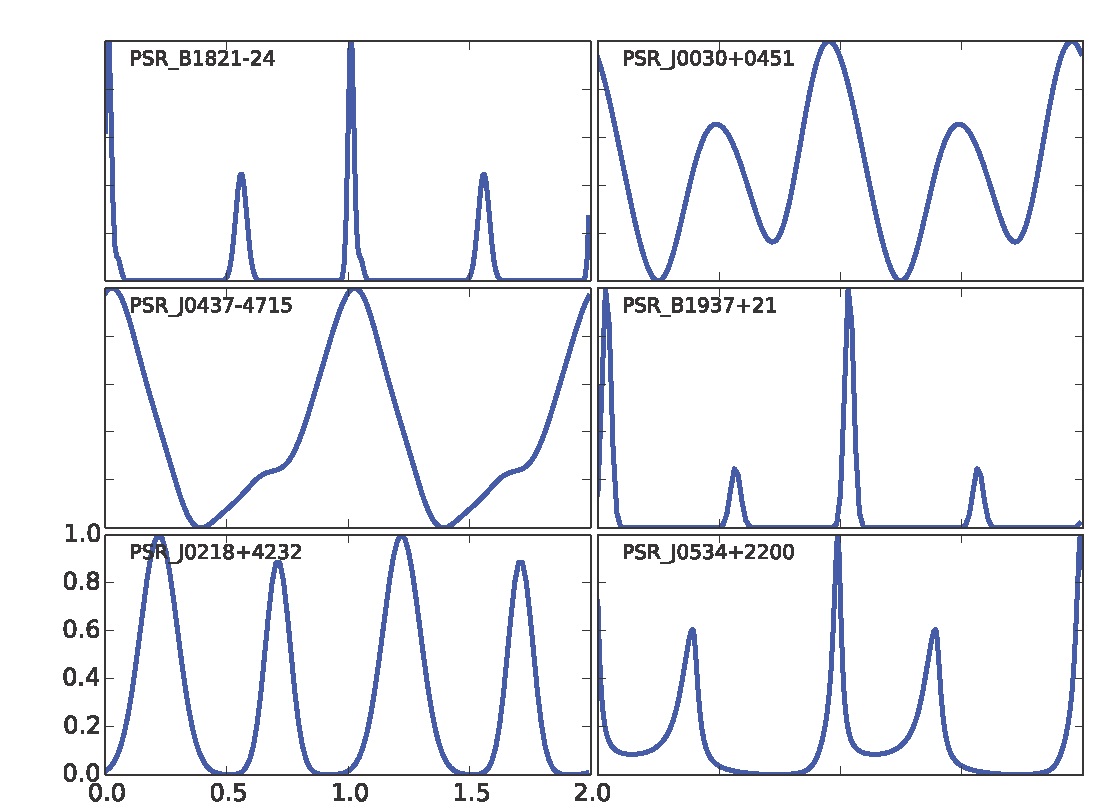
The shape of pulsed signals of a pulsar is called profile in the pulsar astronomy community. Each pulsar has a unique profile, just like the fingerprint of a person. Fig.1(Mitchell et al., ) shows the profiles of pulsars that are selected by the Station Experiment for X-ray Timing and Navigation Technology (SEXTANT) program, which will be introduced in Section 3.2.1.

Figure 1: X-ray pulse profiles of pulsars for SEXTANT program(Mitchell et al., )

2.2 Coordinate and time systems for XNAV

In the aerospace engineering, the orbit motion of spacecraft is described in a coordinate system. XNAV employs the coordinate systems identical to other navigation systems, including (A) the J2000.0 Earth-centered inertial coordinate system for Earth-orbiting spacecraft and (B) the J2000.0 heliocentric-ecliptic coordinate system for deep space spacecraft(Hintz, 2015).

Given that pulsars locate far away from the solar system, there are numerous huge celestial bodies between pulsars and spacecraft. Given that the space is warped by the gravity of the celestial bodies, the time system for XNAV should take the general relativity effect into consideration. As a consequence, the time system for XNAV is the Barycentric Dynamic Time (TDB) or Barycentric Coordinate Time (TCB) (IAU SOFA Center, 2014).

3 Past, present and future projects concerning XNAV

Since the first proposal of pulsar navigation and timing(Downs, 1974; Chester and Butman, 1981), there have been XNAV related projects in the US, China, and Europe. This section will briefly review these projects in chronological order.

3.1 Past projects

3.1.1 USA experiment

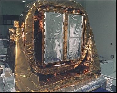
The Unconventional Stellar Aspect (USA) experiment is one of the nine experiments on board the Air Force Space Test Program’s Advanced Research and Global Observation Satellite (ARGOS) launched in 1999, and operated from May 1, 1999, to November 16, 2000. This experiment consisted of a pair of gas scintillation proportional counters to detect X-ray radiations (Ray et al., 2001) (see Fig.2) and a Global Positioning System (GPS) receiver for recording the arrivals of X-ray photons.

The USA experiment diagnosed and corrected a problem with the attitude control of the ARGOS by observing an X-ray source (Kowalski et al., 2001; Wood and Ray, 2017), and tried to fulfill the timekeeping using the observation on Crab pulsar (Wood, 1993a).

Figure 2: Illustration of USA instrument (image credit: Naval Research Laboratory of the United States)

3.1.2 XNAV program

The Defense Advanced Research Projects Agency (DARPA) of the United States started a program, X-ray Source Based Navigation for Autonomous Position Determination, which is also referred to as the XNAV program, in 2004. The XNAV program aimed to develop a revolutionary attitude and navigation capability exploiting periodic celestial sources such as pulsars in the X-ray band (Beckett, 2006).

This program was conceived to last from 2005 to 2010, consisting of three phases. At the end of the program, a flight experiment XNAV was planned to perform on the International Space Station (ISS). However, the whole program was terminated at the end of Phase I (September 2006). Nevertheless, this program performed an in-depth investigation on the feasibility of XNAV, and realized the following achievements (Beckett, 2006):

1. Identifying more than 10 candidate pulsars, whose spin stabilities and X-ray fluxes are capable for precise navigation purpose.

2. Complementation of X-ray detector developments.

3. Demonstrating navigation algorithms for spacecraft position/velocity determination.

4. Designing the demonstration system architecture planned for ISS flight.

3.1.3 XTIM program

Between 2009 and 2010, DARPA (Sheikh et al., 2011) performed the X-ray Timing (XTIM) seedling program to study the use of pulsars for time transfer and investigate future demo scenarios. The XTIM was envisioned to create a Pulsar Timescale (PT) by combining long-term pulsar observations with an ultra-stable local clock for short-term stability. The designed XTIM system was expected to have the following potential characteristics (Sheikh et al., 2011):

1. Stability: XTIM was based on observations of highly stable pulsars.

2. Autonomy: XTIM would provide users with an independent and precise measurement of time.

3. Universality: The pulsars used by XTIM are celestial sources, making them available to any user, anywhere in the solar system.

3.2 Present missions

3.2.1 NICER/SEXTANT program

The Goddard Space Flight Center (GSFC) of the National Aeronautics and Space Administration (NASA) of the US initialized a science mission, Neutron-star Interior Composition Explorer (NICER), in 2011. The fundamental science of NICER is understanding the ultra-dense matter through observations of neutron stars in the soft X-ray band (Gendreau et al., 2012). Besides the science goal, the NICER mission has a technology demonstration enhancement called Station Experiment for X-ray Timing and Navigation Technology (SEXTANT) (Mitchell et al., ). The object of SEXTANT is to perform a real-time, on-board XNAV-only orbit determination with an accuracy of 10 km in the worst-direction, using up to two weeks of dedicated navigation-focused MSP observations.

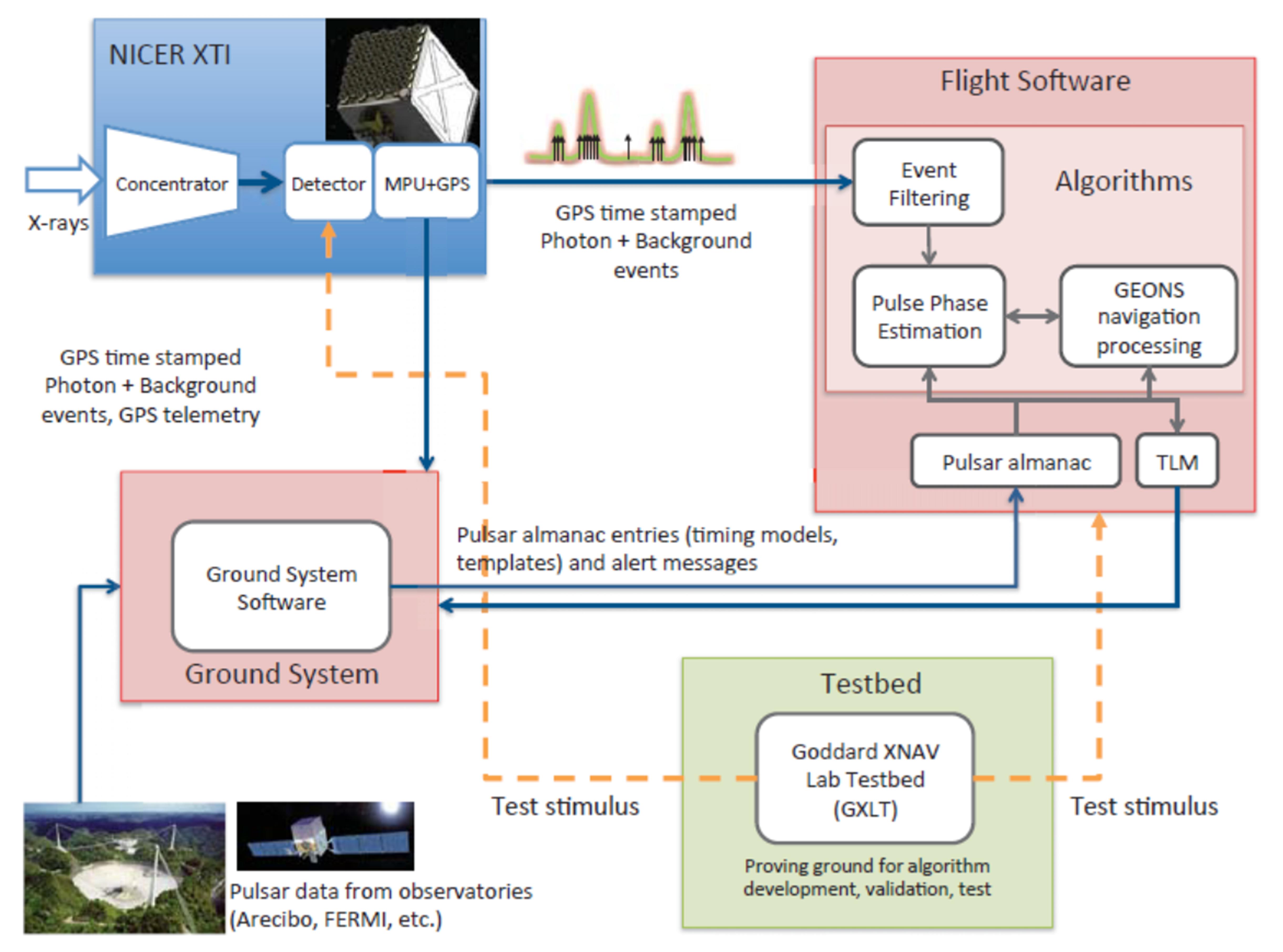
The SEXTANT is the first real-time flight experiment on XNAV in the world. As shown in Fig.3 (Mitchell et al., ), the system architecture of SEXTANT includes four main components: (A) the NICER X-ray Timing Instrument (XTI), (B) the flight software and algorithms, (C) the ground system, and (D) the ground testbed(Mitchell et al., 2014). In 2018, SEXTANT has successfully demonstrated the XNAV aboard the ISS and achieved a positioning error below 10 km (Witze, 2018).

Figure 3: SEXTANT system architecture (Mitchell et al., )

3.2.2 PULCHRON project

In December 2018, the European Space Agency (ESA) announced a project called PULCHRON, an abbreviation built with the words “Pulsar” and “Chronos”, the ancient Greek term for “Time” (Piriz et al., 2019). The primary object of PULCHRON is to demonstrate the effectiveness of a pulsar time scale for the generation and monitoring of system timing in Positioning, Navigation and Timing (PNT) in general, and of Galileo System Time (GST) in particular.

The PULCHRON project is composed of (A) Pulsar Measurement Collection System (PMCS), (B) Pulsar Frequency Standard Unit (PFSU) and (C) Pulsar-Augmented Clock Ensemble (PACE) (Garbin et al., 2019), where PMCS monthly collects the pulsar measurements from the European Pulsar Timing Array (EPTA), which includes Effelsberg, Lovell, Westerbork, Nançay and Sardinia (Ferdman et al., 2010); PFSU aims to realize the physical pulsar time scale; and PACE builds a posteriori "paper" time scale mixing pulsar data and GNSS station and satellite clocks.

3.2.3 XPNAV-1 satellite

China launched an experiment satellite called X-ray Pulsar navigation-1 (XPNAV-1) in November 2016. The objective of XNAV-1 is to test the technology of pulsar observation in the soft X-ray band with the X-ray instruments developed by China Academy of Space Technology (CAST) (Zhang et al., 2017).

Up to now, the XPNAV-1 has accomplished observations on 4 isolated RPPs and 4 X-ray binaries (Zhang et al., 2017), performed a rough orbit determination with an averaged accuracy about 38.4 km (Huang et al., 2019), and completed a timely observation on the glitch of Crab pulsar (Huang et al., 2017).

3.2.4 Navigation study of POLAR

POLAR was a hard X-ray polarimeter aboard the Chinese space laboratory TianGong-2 (TG-2), which was launched in 2016 and deliberately de-orbited in July 2019. It was equipped with an array of 1600 plastic scintillators for precisely and efficiently measuring the linear polarization of hard X-rays. During the mission, POLAR detected 55 $\gamma$-ray bursts.

Besides observing the $\gamma$-ray bursts, POLAR performed a navigation study. The orbit of TG-2 was determined to have an accuracy of about 10 km with 31-day-long hard X-ray data on Crab pulsar. The feasibility of XNAV was validated in principle (Zheng et al., 2017).

3.2.5 Navigation study of Insight-HXMT

The Insight-Hard X-ray Modulation Telescope (Insight-HXMT), China’s first X-ray astronomy satellite, was launched in June 2017. The main scientific objectives of Insight-HXMT include: (A) scanning the Galactic Plane to find new transient sources and to monitor the known variable sources, (B) observing X-ray binaries to study the dynamics and emission mechanism in strong gravitational or magnetic fields, and (C) monitoring and studying Gamma-Ray Bursts (GRBs) and Gravitational Wave Electromagnetic counterparts (GWEM) (Zhang et al., 2020).

Besides accomplishing the scientific objects, Insight-HXMT completed a flight study on XNAV by employing the X-ray data of the Crab pulsar collected between August 30 and September 3, 2017. As a result, it was claimed that Insight-HXMT can locate itself with an error below 10 km (3 $\sigma$)(Zheng et al., 2019; Sun et al., 2022).

3.3 Future missions

3.3.1 CubeX

The SEXTANT team is working with scientists from Smithsonian Astrophysical Observatory and Harvard University to test XNAV on a CubeSat mission called CubeX. CubeX plans to employ an X-ray telescope to identify and spatially map lunar crust and mantle materials excavated by impact craters, and also serves as a pathfinder for autonomous precision deep space navigation using X-ray pulsars (Romaine et al., 2018).

3.3.2 XNavSat

The Indian Institute of Space Science and Technology is developing a small satellite mission called XNavSat. This mission aims to calculate the true anomaly of the satellite in real time, assuming that the remaining orbital elements of the satellite are known (Kandala et al., 2021).

4 Principle of XNAV

4.1 XNAV for a single spacecraft

The basic idea of XNAV for a single spacecraft is similar to that of GNSS. When a spacecraft receives signals from a pulsar, the TOAs of the signals, $t_{\mathrm{SC}}$, can be measured.

Given that the spin frequency of pulsar is stable, the evolution of the pulse phase of pulsar at the Solar System Barycenter (SSB) can be described by

$$\phi\left(t_{\mathrm{SSB}}\right)=\phi_{T_{0}}+\sum^{3}_{i=1}\frac{F_{i-1}}{i!}\left(t_{\mathrm{SSB}}-T_{0}\right)^{i}$$ (2)

where $F_{0}$, $F_{1}$ and $F_{2}$ are the spin frequency of the pulsar at $T_{0}$, its time derivative and its second order time derivative respectively. $\phi_{T_{0}}$ is the phase at $T_{0}$. In practice, $F_{0}$, $F_{1}$ and $F_{2}$ can be found in the public pulsar ephemerides (Alam et al., 2021; Lyne et al., 1993).

Eq.(2) is essentially a Taylor expansion of the pulse phase around the pulse phase at $T_{0}$. If the high orders of the time derivatives of the spin frequency of a pulsar are taken into consideration, the pulse phase evolution should be described more accurately than Eq.(2). However, in practice, the spin frequency and its time derivative families are fitted by the real pulsar data. Up to now, the observation on pulsar has lasted for 55 years (Rea, 2017), and the current pulsar ephemerides only contain the second-order time derivative of spin frequency at most.

In Eq.(2), $t_{\mathrm{SSB}}$ is expressed as Edwards et al. (2006)

$$t_{\mathrm{SSB}} =t_{\mathrm{SC}}+\frac{1}{c}\bm{n}^{\mathrm{T}}\bm{r}_{\mathrm{SSB}}(t)$$ (3)

$$+2\sum_{k}\frac{GM_{k}}{c^{3}}\ln\left(\bm{n}^{\mathrm{T}}\bm{r}_{k}(t)+\left\|\bm{r}_{k}(t)\right\|\right)$$

where $\bm{r}_{\mathrm{SSB}}(t)$ is the position of the spacecraft relative to the SSB, $\bm{n}$ denotes the direction vector of the pulsar, $G$ is the gravitational coefficient, $M_{k}$ is the mass of the $k$th celestial body, $\bm{r}_{k}(t)$ is its position relative to the spacecraft, $c$ is the speed of light, and $\left\|\bullet\right\|$ denotes the $\ell_{2}$-norm of the vector within.

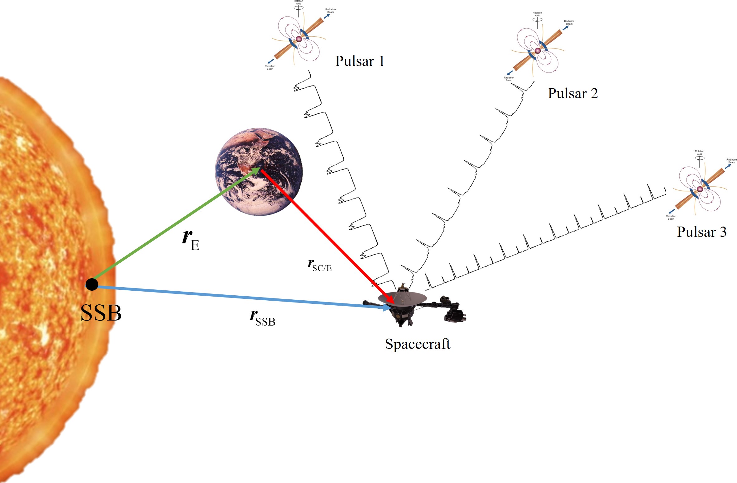
It can be learned from Eq.(3) that $\bm{r}_{\mathrm{SSB}}(t)$ projected on the direction of pulsar, $\bm{n}^{\mathrm{T}}\bm{r}_{\mathrm{SSB}}(t)$, can be obtained if $t_{\mathrm{SSB}}$ and $t$ are available. When the spacecraft receives signals from three pulsars simultaneously (see Fig.4), $\bm{r}_{\mathrm{SSB}}(t)$ can be determined via a nonlinear least squares method just like the way to determine the position via GNSS (Buist et al., 2011). If there are not three pulsars available at the same time, the position of the spacecraft can be estimated by combining the orbit dynamics information with pulsar signals (Zheng and Wang, 2020).

Figure 4: Principle of XNAV for a single spacecraft

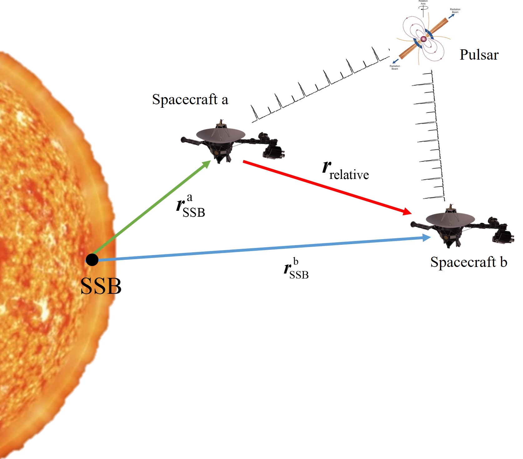
4.2 XNAV for multi-spacecraft

Fig.5 shows two spacecraft observing one pulsar. Assume $t_{\mathrm{SC}}^{\mathrm{A}}$ and $t_{\mathrm{SC}}^{\mathrm{B}}$ are the pulse TOAs at spacecraft A and spacecraft B, respectively. According to Eq.(3), we have

$$t_{\mathrm{SSB}}^{\mathrm{A}}-t_{\mathrm{SSB}}^{\mathrm{B}} =t_{\mathrm{SC}}^{\mathrm{A}}-t_{\mathrm{SC}}^{\mathrm{B}}$$ (4)

$$+\frac{1}{c}\bm{n}^{\mathrm{T}}\left(\bm{r}_{\mathrm{SSB}}^{\mathrm{A}}(t_{\mathrm{SC}}^{\mathrm{A}})-\bm{r}_{\mathrm{SSB}}^{\mathrm{B}}(t_{\mathrm{SC}}^{\mathrm{B}})\right)$$

$$+2\sum_{k}\frac{GM_{k}}{c^{3}}\ln\frac{\bm{n}^{\mathrm{T}}\bm{r}_{k}^{\mathrm{A}}(t_{\mathrm{SC}}^{\mathrm{A}})+\left\|\bm{r}_{k}^{\mathrm{A}}(t_{\mathrm{SC}}^{\mathrm{A}})\right\|}{\bm{n}^{\mathrm{T}}\bm{r}_{k}^{\mathrm{B}}(t_{\mathrm{SC}}^{\mathrm{B}})+\left\|\bm{r}_{k}^{\mathrm{B}}(t_{\mathrm{SC}}^{\mathrm{B}})\right\|}$$

where $\bm{r}_{k}^{\mathrm{A}}$ and $\bm{r}_{k}^{\mathrm{B}}$ are the positions of the $k$th celestial body relative to the spacecraft A and B, respectively.

In most cases, $\bm{r}_{k}^{\mathrm{A}}\approx\bm{r}_{k}^{\mathrm{B}}$ given that the distance between the two spacecraft is far less than the distances between the celestial bodies and the spacecraft. Thus, $\ln\frac{\bm{n}^{\mathrm{T}}\bm{r}_{k}^{\mathrm{A}}(t_{\mathrm{SC}}^{\mathrm{A}})+\left\|\bm{r}_{k}^{\mathrm{A}}(t_{\mathrm{SC}}^{\mathrm{A}})\right\|}{\bm{n}^{\mathrm{T}}\bm{r}_{k}^{\mathrm{B}}(t_{\mathrm{SC}}^{\mathrm{B}})+\left\|\bm{r}_{k}^{\mathrm{B}}(t_{\mathrm{SC}}^{\mathrm{B}})\right\|}$ in Eq.(4) is close to 0. As a consequence, Eq.(4) can be rewritten as

$$t_{\mathrm{SSB}}^{\mathrm{A}}-t_{\mathrm{SSB}}^{\mathrm{B}} =t_{\mathrm{SC}}^{\mathrm{A}}-t_{\mathrm{SC}}^{\mathrm{B}}$$ (5)

$$+\frac{1}{c}\bm{n}^{\mathrm{T}}\left(\bm{r}_{\mathrm{SSB}}^{\mathrm{A}}(t_{\mathrm{SC}}^{\mathrm{A}})-\bm{r}_{\mathrm{SSB}}^{\mathrm{B}}(t_{\mathrm{SC}}^{\mathrm{B}})\right)$$

As shown in Eq.(5), assuming $\bm{r}_{\mathrm{SSB}}^{\mathrm{A}}(t_{\mathrm{SC}}^{\mathrm{A}})-\bm{r}_{\mathrm{SSB}}^{\mathrm{B}}(t_{\mathrm{SC}}^{\mathrm{B}})=\bm{r}_{\mathrm{Relative}}$, $\bm{r}_{\mathrm{SSB}}^{\mathrm{A}}(t_{\mathrm{SC}}^{\mathrm{A}})$, $\bm{r}_{\mathrm{SSB}}^{\mathrm{B}}(t_{\mathrm{SC}}^{\mathrm{B}})=\bm{r}_{\mathrm{Relative}}$ and $\bm{r}_{\mathrm{Relative}}$ can be estimated when three pairs of $t_{\mathrm{SSB}}^{\mathrm{A}}-t_{\mathrm{SSB}}^{\mathrm{B}}$ and $t_{\mathrm{SC}}^{\mathrm{A}}-t_{\mathrm{SC}}^{\mathrm{B}}$ from three pulsars are available simultaneously or sequentially (Emadzadeh and Speyer, 2011; Xiong et al., 2009).

Figure 5: Principle of XNAV for multi-spacecraft

4.3 Techniques supporting XNAV

As shown in Eqs.(2), (3) and (5), the techniques supporting XNAV are:

1. Navigation pulsar database: Pulsars for XNAV are like navigation satellites for GNSS. Unlike the man-made satellites, the location, brightness and modulation properties of pulsars cannot be designed. Thus, pulsars qualified for navigation are rare and their ephemerides need to be updated timely.

2. X-ray detection system: X-ray detection system for XNAV are like GNSS receivers for GNSS. They detect and record X-ray photons from pulsars.

3. Pulse TOA estimation: Pulse TOA is an important and basic parameter for XNAV, as illustrated in Eqs.(3) and (5). However, a spacecraft can only record a series of photons instead of a continuous pulsed signal given that the flux of a pulsar is extremely weak. Moreover, the spacecraft keeps performing an orbit motion, which causes the extraction of pulse TOA from the recorded photons more complex. As a consequence, it is a great challenge to get a reliable and precise pulse TOA.

The advances of the above three techniques will be sequentially introduced in Sections 5-7.

5 Navigation pulsar database

As illustrated in Section 2.1.1, RPPs are recommended for navigation. Currently, 2200 RPPs have been discovered (Manchester et al., 2005), among which about 150 pulsars emit X-ray radiation (Becker, 2009). Approximately 10% pulsars are MSPs (Becker et al., 2013). MSPs are the most promising reference sources for XNAV because they exhibit very high timing stabilities, which are comparable to the current atomic clocks (Taylor, 1991; Matsakis et al., 1997).

Table 1 shows the navigation X-ray pulsars used by the past and present missions. The Crab pulsar (or PSR B0531+21) is selected by all missions. Although the Crab pulsar is not a MSP and has glitches in which the spin parameters change suddenly (Shaw et al., 2018), it is much brighter in X-ray than the other pulsars. Therefore, the Crab pulsar can be easily detected and can provide a much more accurate pulse TOA than MSPs when the Crab pulsar and MSPs are observed for the same duration.

The navigation pulsar database contains the following information that describes the timing and location properties of the selected pulsars:

1. Position parameters including the declination, the right ascension, and the proper motion of pulsar;

2. Frequency evolution parameters including the spin frequency and its first- and second-order time derivatives;

3. The other necessary parameters including the absolute pulse phase for a given epoch, the version of planet ephemerides (NASA’s Jet Propulsion Laboratory (JPL) ephemerides for example) , the orbit parameters of binary pulsars, etc.

In practice, the navigation pulsar database is supported by the pulsar timing analysis, which is usually performed by global pulsar timing programs. For example, the North American Nanohertz Observatory for Gravitational Waves (NANOGrav) project (McLaughlin, 2013) has been timing several pulsars in the pulsar database of SEXTANT program (Ray et al., 2017), the Jodrell Bank observes the Crab pulsar (Lyne et al., 1993), and the Parkes Pulsar Timing Array (PPTA) monitors 20 pulsars (Reardon et al., 2016).

Table 1: X-ray navigation pulsars selected by past and present missions

Mission	X-ray pulsars selected for navigation
USA experiment(Wood and Ray, 2017)	Crab pulsar
XNAV program(Sheikh et al., 2006)	PSR B1937+21, PSR B1957+20, SAX J1808.4-3658, PSR B1821-24, XTE J1751-305, XTE J1807-294
	Crab pulsar, PSR B0540-69
SEXTANT program(Ray et al., 2017)	PSR B1937+21, PSR B1821-24, PSR J0218+4232, PSR J0030+0451, PSR J1012+5307, PSR J0437-4715
	PSR J2124-3358, PSR J0751+1807, PSR J1024-0719, PSR J2214+3000, Crab pulsar
XPNAV-1(Huang et al., 2019)	Crab pulsar
Insight-HXMT(Zheng et al., 2019)	Crab pulsar

6 X-ray detection system

The pulse X-ray emission of a RPP is usually non-thermal, which has a power law spectrum with a photon index of about $-2$, i.e., the flux of the pulse photon in the soft X-ray band (photon energy less than 10 kilo electron Volt (keV)) is much higher than that in the hard X-ray band (energy above 10 keV) (Sheikh et al., 2006; Kalemci, 2018). More photons indicate a more accurate pulse TOA estimation (see Section 7). Therefore, the soft X-ray radiation from pulsars is recommended for navigation. The background, which comes from the diffuse Cosmic X-ray Background (CXB), space particles and the non-pulse portion of the pulsar, is commonly detected along with the X-rays of pulsars (Kalemci, 2018). As a consequence, an X-ray detection system consists of an optics system, designed to focus X-ray photons, and an X-ray detector counting X-ray photons collected by the optics system.

6.1 Optics system

Two broad categories of optics systems are used in XNAV observations: collimators and focusing X-ray telescopes. A collimator restricts the Field of View (FOV) of the whole detection system. In this way, only the background within a narrow portion of the space can enter the detection system. On the other hand, a focusing X-ray telescope focuses the source flux onto the X-ray detector in the focal plane (Ramsey et al., 1993). As will be seen in Section 6.1.2, only the background arriving within a small incidence angle can be collected. Therefore, both the collimator and focusing X-ray telescope can effectively reduce the background.

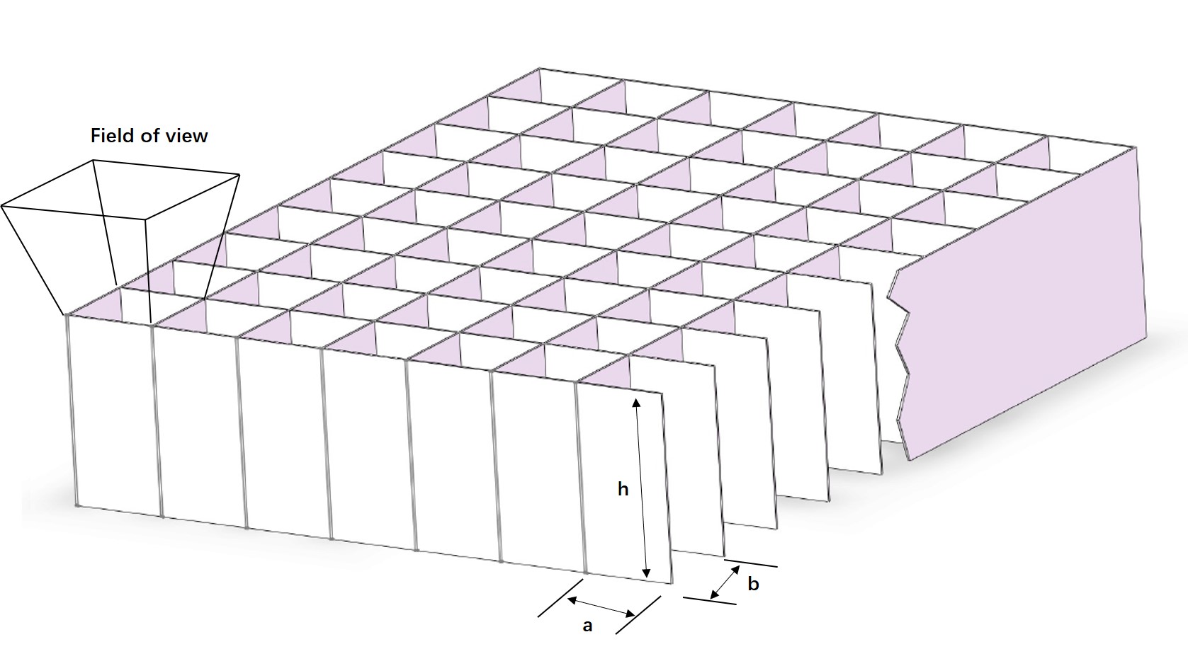
6.1.1 Collimators

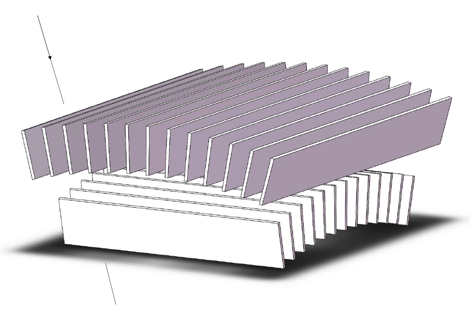
Fig.6(Ramsey et al., 1993) shows a simple slat collimator with an FOV of $\mathrm{arctan}\left(a/h\right)\times\mathrm{arctan}\left(b/h\right)$ where $a$, $b$ and $h$ are the length, width, and height of a slat respectively. All photons or particles arriving at angles larger than $\mathrm{arctan}\left(a/h\right)$ and $\mathrm{arctan}\left(b/h\right)$ are attenuated by the walls of collimator structure. In other words, the photons or particles from the sources with angular positions relative to the targeted source outside the FOV are rejected. Thus, for collimators, a small FOV indicates a strong capability of rejecting background.

Because of their simple structures, collimators were used in a number of X-ray missions including Uhuru, the first X-ray satellite launched in 1970 (Fabian, 1975) (see Table 2(Fabian, 1975; Giacconi et al., 1971; Sanford, 1974; Gursky et al., 1978; Rothschild et al., 1979; Turner et al., 1981, 1989; Jahoda et al., 2006; Zhang et al., 2020; Smith and Courtier, 1976)). Collimators are also used in X-ray imaging, with scanning observations and image reconstruction techniques (Bradt et al., 1968).

Figure 6: A simple slat collimator (Ramsey et al., 1993)

Table 2: Past and active X-ray telescopes employing collimators

Spacecraft	Year	Instrument	Optics system		Detector	Total effective area ($\mathrm{cm^{2}}$)
			FOV	Energy range (keV)
Uhuru (Fabian, 1975; Giacconi et al., 1971)	$1970-1973$	-	$0.52^{\circ}\times 0.52^{\circ}$ and $5.2^{\circ}\times 5.2^{\circ}$	2-20	Proportional counter	1680
Ariel V(Smith and Courtier, 1976)	$1974-1980$	LE	$0.75^{\circ}\times 10.6^{\circ}$	1.2-5.8	Proportional counter	145
		HE	$0.75^{\circ}\times 10.6^{\circ}$	2.4-19.8	Proportional counter	145
OAO-3(Sanford, 1974)	$1972-1981$	-	$2.5^{\circ}\times 3.5^{\circ}$	2.5-10	Proportional counter	17.8
HEAO-1(Gursky et al., 1978; Rothschild et al., 1979)	$1977-1979$	LASS	varied between $1^{\circ}\times 4^{\circ}$ and $1^{\circ}\times 0.5^{\circ}$	0.25-25	Proportional counter	$7\times(1350-1900)$
		CEX		0.15-3.0	Proportional counter	$2\times 400$
			various setting: $1.5^{\circ}\times 3^{\circ}$, $3^{\circ}\times 3^{\circ}$, $3^{\circ}\times 6^{\circ}$	1.5-20	Proportional counter	800
				2.5-60	Proportional counter	$3\times 800$
		MC	$4^{\circ}\times 4^{\circ}$	0.9-13.3	Proportional counter	$400$
					Proportional counter	$300$
EXOSAT(Turner et al., 1981)	$1983-1986$	ME	$45^{\prime}\times 45^{\prime}$	1.3-15, 5-55	Proportional counter	$1800$
Ginga(Turner et al., 1989)	$1987-1991$	LAC	$0.8^{\circ}\times 0.7^{\circ}$	1.5-30	Proportional counter	$4000$
RXTE(Jahoda et al., 2006)	$1995-2012$	PCA	$1^{\circ}$	2-60	Proportional counter	$6500$
Insight-HMXT(Zhang et al., 2020)	$2017-$	LE	$15\times(1.1^{\circ}\times 5.7^{\circ})$ and $2\times(5.7^{\circ}\times 5.7^{\circ})$	1-12	SCD	$384$
		ME	$16\times(1^{\circ}\times 4^{\circ})$ and $2\times(4^{\circ}\times 4^{\circ})$	8-35	Si-PIN	$952$
		HE	$16\times(1.1^{\circ}\times 5.7^{\circ})$ and $2\times 5.7^{\circ}\times 5.7^{\circ}$	20-350	NaI(CsI)	$5100$

1) Note: HEAO-1 $-$ High Energy Astronomy Observatory-1; EXOSAT $-$ European X-ray Observatory SATellite; RXTE $-$ Rossi X-ray Timing Explorer; LE $-$ Low Energy system, HE $-$ High Energy system; LASS $-$ Large Area Sky Survey experiment; LAC $-$ Large Area Proportional Counter; CXE $-$ Cosmic X-ray Experiment; PCA $-$ Proportional Counter Array

6.1.2 Focusing X-ray telescopes

X-rays can be focused with the grazing incidence optics. The mirrors comprising focusing X-ray telescopes are typically multi-shell like structures coated with a heavy metal, such as gold or nickel (Smith, 2006). Soft X-ray photons can be reflected from the surface of mirror, when their angles of incidence with respect to the surface are less than (Ade et al., 2022)

$$\theta_{\mathrm{c}}=37\frac{\rho^{1/2}}{E}$$ (6)

where $\rho$ is the density of coating material and $E$ is the energy of photon.

The reflectivity of gold is a function of energy and angle of incidence(Ade et al., 2022), which increases as the energy and angle of incidence reduce. In practice, the angle of incidence is typically less than $1^{\circ}$. However, a low angle of incidence can be achieved at the cost of a long focal length of the telescope.

In order to achieve a good reflectivity and good imaging quality, focusing X-ray telescopes require much precise figuring and ultra-high-quality mirrors with roughness better than 1 nm (Ramsey et al., 1993). The above requirements all indicate that the fabrication of focusing X-ray telescopes is expensive and labor-intensive.

For a focusing X-ray telescope, its effective area depends on the energies of incoming photons because the reflectivity is a function of photons’ energies and thus is with the unit of "$\mathrm{cm}^{2}@b\mathrm{keV}$", where $@b\mathrm{keV}$ means "at $b$ $\mathrm{keV}$". Besides this, the angular resolution quantified by the Half-Power Diameter (HPD) is also an important parameter to describe the imaging capability of a focusing telescope(O’Dell et al., 2010). HPD is defined as the angular diameter in the focal plane, which contains half the flux (at a given energy) focused by the telescope.

Although there are various geometries that can achieve grazing incidence optics (Gorenstein P, 2012), the Wolter-I geometry is most frequently used in X-ray telescopes (see Table 3(Tousey, 1977; Giacconi et al., 1979; Taylor et al., 1981; Korte et al., 1981; Aschenbach, 1988; O’Dell et al., 2010; Serlemitsos et al., 1995; Gorenstein, 2010; Smith, 2006; Lumb et al., 2012; Burrows et al., 2005; Serlemitsos et al., 2007; Harrison et al., 2013; Singh et al., 2014; Takahashi et al., 2018; Sato et al., 2016; Li et al., 2018; Okajima et al., 2016; Friedrich et al., 2008; Pavlinsky et al., 2021)). Since the FOV of a Wolter-I geometry is small, recently, a lobster-eye geometry is used to achieve wide field X-ray imaging. A lobster-eye geometry can observe simultaneously multiple sources locating relative far away, such as $10^{\circ}$ from each other, and can monitor transient X-ray sources. This section will focus on the two geometries.

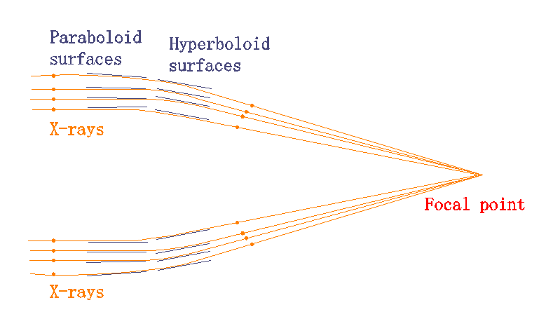
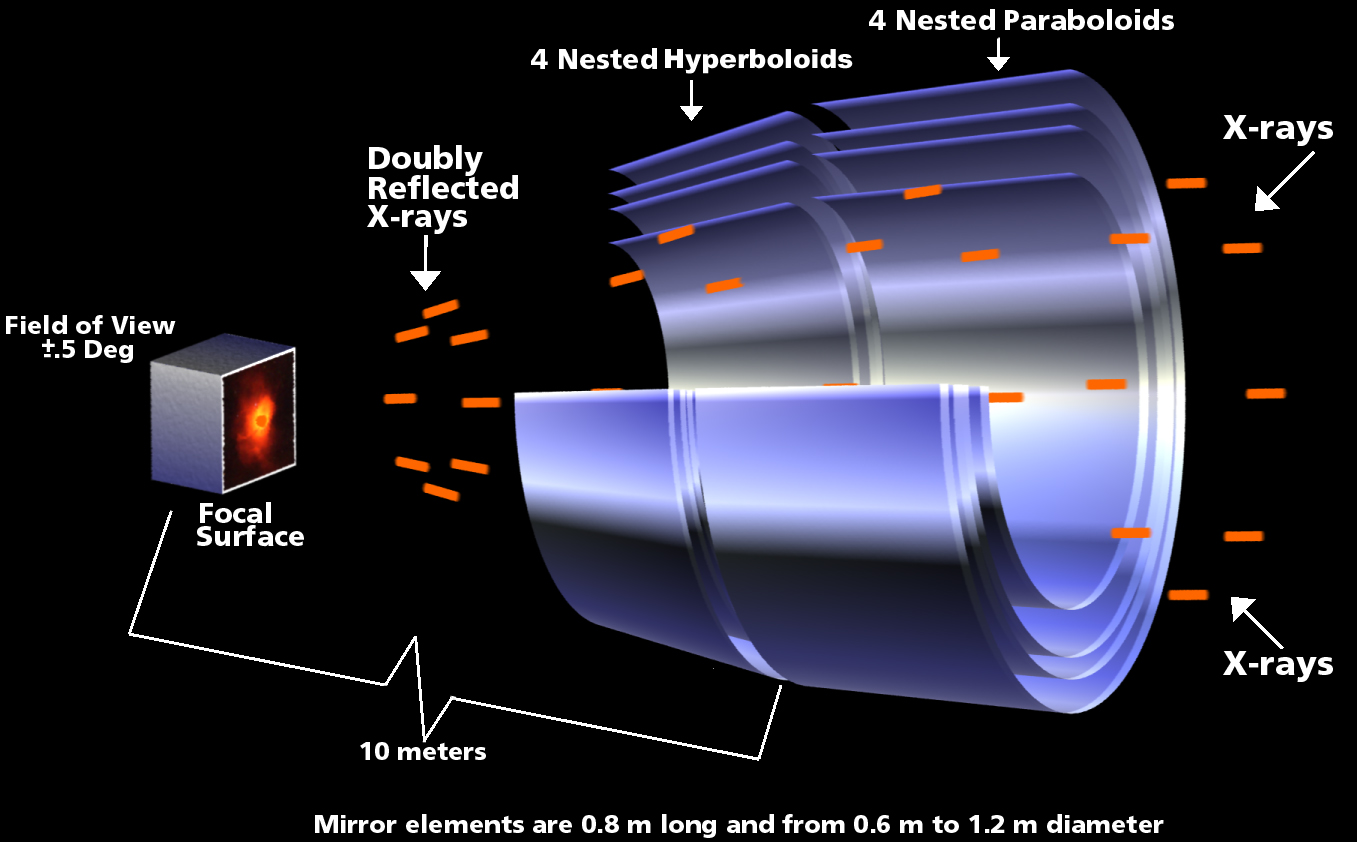
(1) Wolter-I geometry

Almost the focusing X-ray telescopes that have been in orbit were fabricated in accordance with or approximating the Wolter-I geometry (Gorenstein, 2010) with the principle shown in Fig.7 (Wolter, 1952). The incoming rays experience two grazing incidence reflections from two confocal paraboloidal and hyperboloidal mirrors sections. Several pairs of paraboloidal and hyperboloidal mirrors can be nested to increase the effective area. Fig.8 shows the nested mirrors on the Chandra X-ray Observatory.

Figure 7: Principle of Wolter-I geometry(Wolter, 1952)

Figure 8: Nested X-ray mirrors on Chandra X-ray Observatory (Image credit: NASA, Chandra, and the Smithsonian Astrophysical Observatory.)

Table 3: Past and active X-ray telescopes using Wolter-I geometry

Spacecraft	Year			Optics system
		Instrument	Energy range	Angular resolution/HPD	Focal length	Reflecting	Number of*	Detector	Total effective area
			(keV)		(m)	surface	nested shells	on the focal plane
Skylab(Tousey, 1977)	1973$-$1974	ATM	0.23-4.1	3"	1.903	Fused silica	1	Proportional counter	9 $\mathrm{cm}^{2}@1\mathrm{keV}$
HEAO-2 (Einstein)(Giacconi et al., 1979)	1978$-$1981		0.2-4	4"	3.4	quartz	4	Proportional counter	$400\mathrm{cm}^{2}@0.25$ keV
EXOSAT(Taylor et al., 1981; Korte et al., 1981)	1983$-$1986	LE	0.05-2	24"	0.28	Gold	4	Proportional counter	$38\mathrm{cm}^{2}@1.5$keV
ROSAT(Aschenbach, 1988; O’Dell et al., 2010)	1990$-$1999		0.5-1.5	5"	2.4	Gold	4	Proportional counter	$400\mathrm{cm}^{2}@1$keV
ASCA(Serlemitsos et al., 1995)	1993$-$2001		0.4-10	2.9′	3.5	Gold	$4\times 30$	Proportional Counter	$4\times 300\mathrm{cm}^{2}@1$keV
								CCD
Chandra(Gorenstein, 2010; Smith, 2006; O’Dell et al., 2010)	1999$-$		0.1-10	0.5"	10.0	Iridium	4	CCD	$800\mathrm{cm}^{2}@0.25$keV
XMM-Newton(Lumb et al., 2012)	1999$-$		0.1-12	15"	7.5	Gold	$3\times 58$	CCD	$3\times 1500\mathrm{cm}^{2}@1$ keV
Swift(Burrows et al., 2005)	2004$-$		0.2-10	15"	3.5	Gold	12	CCD	$110\mathrm{cm}^{2}@1.5$ keV
Suzaku(Serlemitsos et al., 2007)	2005-	XRT-I	0-10	2′	4.75	Gold	175	CCD	$450\mathrm{cm}^{2}@1.5$keV
		XRT-S			4.5		168	X-Ray Spectrometer	$450\mathrm{cm}^{2}@1.5$keV
NuSTAR(Harrison et al., 2013)	2012$-$		3-78.4	58"	10.14	Platinum/Carbon (inner surface)	133	CdZnTe detector	$847\mathrm{cm}^{2}@9$keV
						Tungsten/Silicon (outer surface)
ASTROSAT(Singh et al., 2014)	2015$-$	SXT	0.3-8	2′	2	Gold	40	CCD	$128\mathrm{cm}^{2}@1.5$keV
Hitomi(Takahashi et al., 2018; Sato et al., 2016)	2016$-$2016	SXI	0.4-12	1.3′	5.6	Gold	203	CCD	$370\mathrm{cm}^{2}@1$keV
XPNAV-1(Li et al., 2018)	2016$-$	iFXPT	0.5-10	15′	1.15	Gold	4	SDD	$2.8\mathrm{cm}^{2}@1$keV
ISS(Okajima et al., 2016)	2017$-$	NICER	0.2-12		1.085	Gold	$56\times 24$	SDD	$1793\mathrm{cm}^{2}@1.5$keV
SRG(Friedrich et al., 2008; Pavlinsky et al., 2021)	2019$-$	ART-XC	4-30	30-35"	2.7	Iridium	28	CdZnTe detector	$385\mathrm{cm}^{2}@8.1$keV
		eROSITA	0.2-10	15"	1.6	Gold	$7\times 54$	CCD	$7\times 300\mathrm{cm}^{2}@1$keV

1) Note: ATM $-$ Apollo Telescope Mount; HEAO-2 $-$ High Energy Astronomy Observatory-2; ROSAT $-$ ROentgen SATellite; ASCA $-$ Advanced Satellite for Cosmology and Astrophysics; Chandra $-$ Chandra X-ray Observatory; XMM-Newton $-$ X-ray Multi-Mirror-Newton; XRT-I $-$ X-ray telescope for X-ray Imaging Spectrometer; XRT-S $-$ X-ray telescope for X-ray Spectrometer; ASTROSAT $-$ Astronomy Satellite; SXT $-$ Soft X-ray Telescope; SXI $-$ Soft X-ray camera; iFXPT $-$ incidence Focusing X-ray Pulsar Telescope; SRG $-$ Spectrum Roentgen Gamma; ART-XC $-$ Astronomical Roentgen Telescope–X-ray Concentrator; eROSITA $-$ extended ROentgen Survey with an Imaging Telescope Array

*) A shell denote a pair of paraboloidal and hyperboloidal mirrors.

$\dagger$) NICER employs only paraboloidal mirrors and cannot image.

(2) Lobster-eye optics

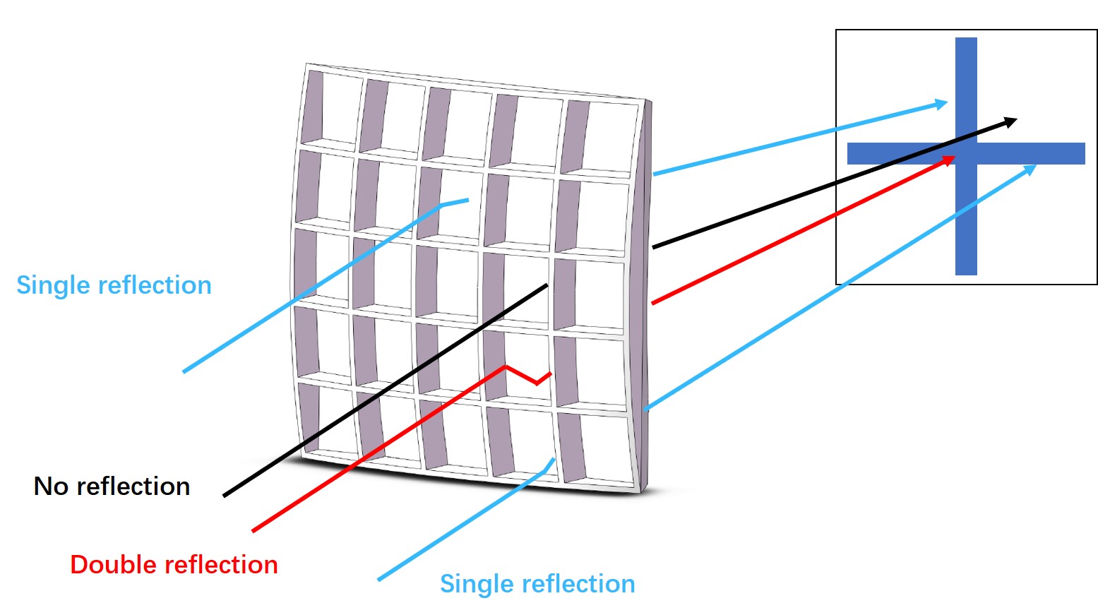
This optics mimics the eyes of lobsters and was suggested independently by Schmidt (Schmidt, 1975) in 1975 and by Angel (Angel, 1979) in 1979. The Schmidt arrangement employs the orthogonal sets of mirrors (see Fig.9) and the Angel arrangement utilizes array of reflecting cells (see Fig.10). The lobster-eye optics has a wide FOV, up to maximum of $2\pi$ (Pina et al., 2019). This feature makes the lobster-eye optics more suitable for the all-sky survey than the Wolter-I geometry, the FOV of which is typically less than $1^{\circ}$ (Gorenstein, 1987; Fraser et al., 2002).

The lobster-eye optics can be constructed as a
one-Dimensional (1D) or two-Dimensional (2D) system. The Schmidt arrangement shown in Fig.9 is a 2D system, which consists of two orthogonal 1D systems. The Angel arrangement is also a 2D system. The incoming photons focused to form a point with tails forming a cross like image, in which the photons at the center point are reflected twice and those in the wings are only reflected once (min Yuan et al., 2018). It appears that the Schmidt arrangement can practically achieve an angular resolution of the order of one tenth of a degree or better, and the angular resolution of the Angel arrangement can be as good as a few arc seconds, if very precise reflecting cells can be fabricated (Pina et al., 2019).

Figure 9: Schmidt arrangement for a lobster-eye geometry

Figure 10: Angel arrangement for a lobster-eye geometry

Nowadays, both the Schmidt and Angel arrangements are under development. Ref.95 designs an X-ray optics system for CubSat demonstrator based on the Schimdt arrangement. Ref.99 uses the microchannel plate technology to fabricate the reflecting cells in the Angel arrangement. Ref.100 employs the micro-pore optics to realize the Angel arrangement.

In the near future, the Einstein Probe (EP) (Yuan et al., 2018b) will employ the lobster-eye optics to form a large FOV monitor to detect X-ray transients and gamma-ray bursts. In order to test the lobster-eye optics for EP, the EP-WXT Pathfinder, an experimental module for the Wide-field X-ray Telescope (WXT) of EP, was loaded on the satellite SATech-01 launched on July 27, 2022. The EP-WXT Pathfinder released on its first results on August 27, 2022. The Space-based multi-band astronomical Variable Objects Monitor (SVOM) (Götz et al., 2009; Feldman et al., 2017) will employ a narrow-field-optimised lobster-eye telescope to promptly detect and accurately locate gamma-ray bursts afterglows. These two satellites will be launched in the next couple of years.

6.2 Detectors

X-ray detectors aim to turn the collected X-rays into electronic signals and further into data that can be stored for later analysis (Arnaud et al., 2011). These data typically include the arrival time, energy, and the location on the detector of each photon detected. The commonly used X-ray detectors are proportional counters, Charge-Coupled Devices (CCDs), Silicon Drift Detectors (SDDs), scintillation detectors, CdZnTe detectors, etc.

6.2.1 Proportional counters

Proportional counters were stemmed from gases detectors, which were first applied to detect cosmic rays and other particles in laboratory (Xu and Brown, 1987), and have been used in soft X-ray astronomy for nearly six decades.

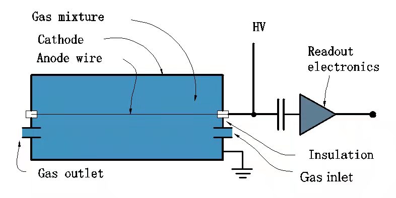
A standard proportional counter is a gas-filled chamber with a coaxial thin wire as shown in Fig.11. The electrical field is generated by applying positive High Voltage (HV) to the anode (Winkler et al., 2015). X-rays entering the chamber ionize the gas, producing electrons. The electrons can be accelerated in the electric field and further ionize gas atoms by collisions and cause charge multiplication. In proportional counter, the HV is tuned to maintain a linear relation between the input photon energy and the charge (Arnaud et al., 2011). This is the very reason for its name.

Figure 11: Schematic diagram of a proportional counter

As shown in Tables 2 and 3, the combinations of proportional counters and collimators were widely applied to X-ray astronomy satellites, especially those launched before 2000. It is because, the observation of the weak photon fluxes from cosmic X-ray sources with non-imaging detection systems (detectors with collimators) requires large-area detectors, which can be realized by multi-anode multilayer proportional counters under the level of fabrication then.

In order to improve the energy resolution of the proportional counter, the Gas Scintillation Proportional Counter (GSPC) was proposed (Conde and Policarpo, 1967) and used aboard the EXOSAT (White, 1990). However, GSPCs have now been superseded by CCDs (see Section 6.2.2) for soft X-ray band and CdZnTe detectors (see Section 6.2.5) for hard X-ray band (Arnaud et al., 2011).

Proportional counters may suffer from an aging problem because of the cracking of gas molecules during normal operation (Trümper and Hasinger, 2008). The USA experiment (see Section 3.1.1) was aborted because of the leakage of gases filled in the proportional counters.

6.2.2 CCD

The CCD was invented at Bell Laboratories in 1969, and was first employed as the focal plane detector for X-ray imaging by the ASCA satellite in 1993. Since then, CCDs are the most widely used detectors in X-ray astronomy because a CCD detector usually has small pixel size, large chip size, good energy resolution, and low noise (Fioretti and Bulgarelli, 2020).

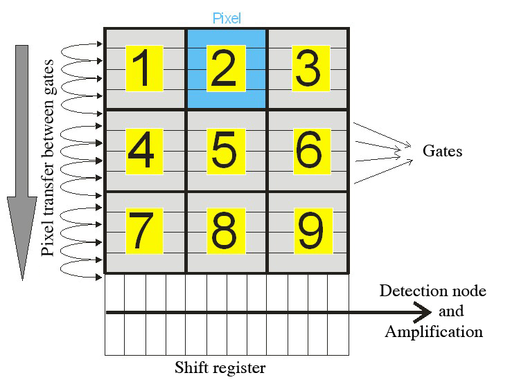
A conventional CCD is an array of small and thin electrodes of metal-oxide-semiconductor capacitors. The incoming X-rays interact with the semiconductor substrate, producing electron-hole pairs. An electric field can be produced, when the gates between neighboring pixels have potentials (Fioretti and Bulgarelli, 2020). In this way, the electrons can be stored in pixels, and can be transferred, pixel to pixel, from the semiconductor to a readout amplifier, by tuning the gate potentials (see Fig.12).

Figure 12: Electrons transfer principle for a $3\times 3$ pixels CCD(CCD, )

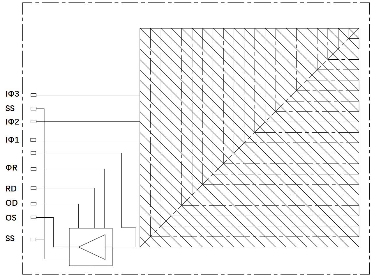
Although CCDs have a high energy resolution up to about 130 eV@ 6keV and a spatial resolution on the order of 10 ${\rm\mu}$m, their read-out typically cost several seconds (Nakajima et al., 2009). In order to accelerate the read-out, two variations on CCD have been designed, including the pnCCD (Ihle et al., 2017) and the Swept Charge Devices (SCD) (Gow et al., 2012). In a pnCCD, the pixels are aligned as column parallel, and each column has a dedicated readout channel (Andritschke et al., 2008; Meidinger et al., 2006). In an SCD, the electrons generated by interactions between X-rays and the semiconductor substrate are simultaneously or consecutively swept towards the central diagonal channel, and then are transferred to the single read-out node located in one corner of the devices (see Fig.13). In this way, an SCD can improve the time resolution at the cost of sacrificing imaging capability (Lowe et al., 2001). Up to now, pnCCD has been applied to the XMM-Newton and eROSITA, and will operate on the SVOM and EP. SCDs have been applied to the Insight-HXMT.

Figure 13: Schematic diagram of SCD

6.2.3 SDD

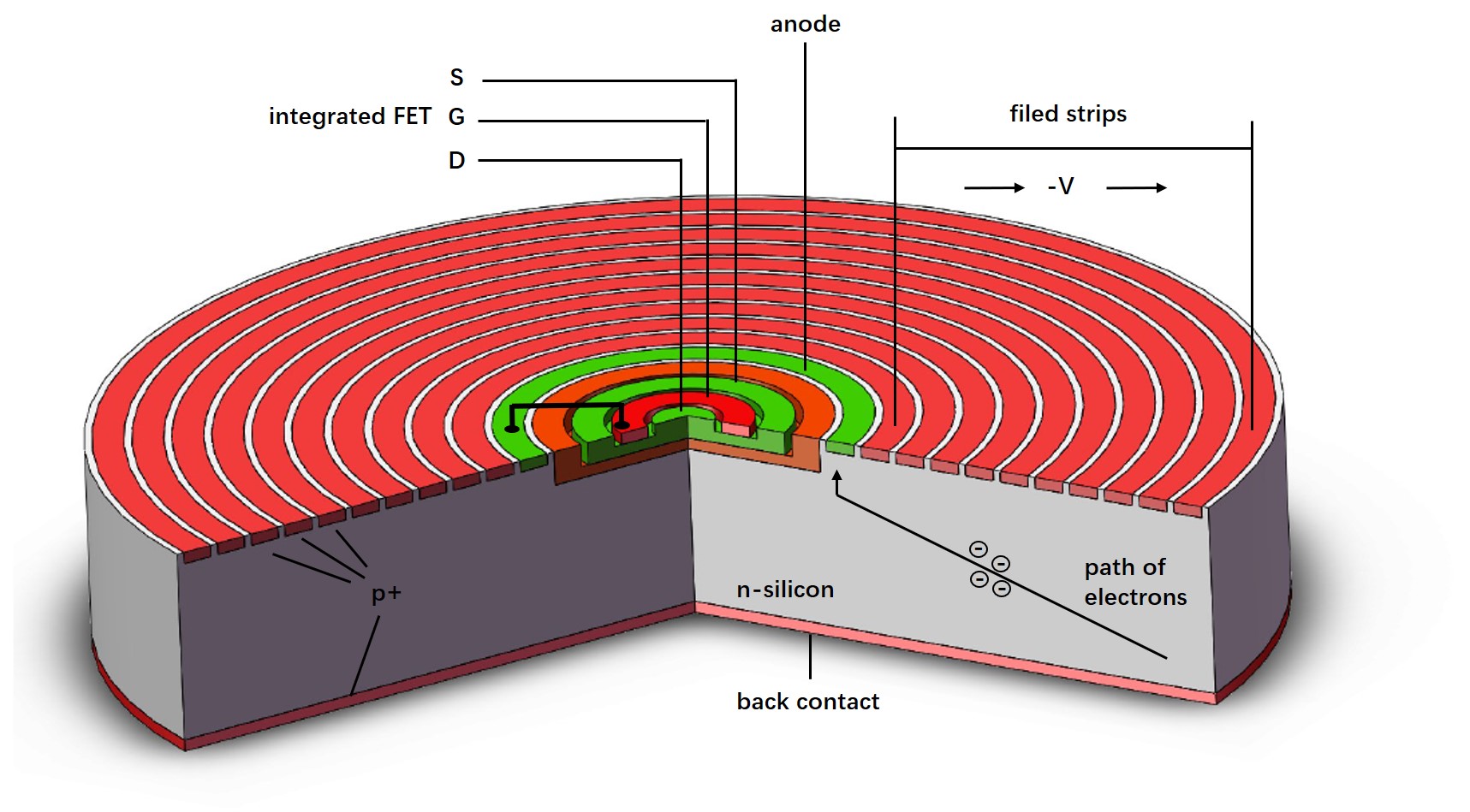
SDDs were first proposed in 1983 (Gatti and Rehak, 1984). An SDD consists of a radial electric field, which terminates in a very small collecting anode on one face of the device (see Fig.14). Electrons generated by the interactions between X-rays and the semiconductor are guided along these electric field lines to the anode. On the other hand, a small anode indicates a low device capacitance, and finally produces a small electronic noise (Takahashi et al., 2001). Electrons move fast in the electric field, and so can be collected in a very short time. SDDs thus have a very high time resolution. However, one SDD pixel needs one read-out channel, which makes it almost impossible to obtain high spatial resolution images like CCDs.

SDDs have been successfully applied to NICER and XNAV-1, and are planned to be employed by CubeX, XNavSat and the enhanced X-ray Timing and Polarimetry (eXTP) (Zhang et al., 2016).

Figure 14: Schematic diagram of SDD

6.2.4 Scintillation detector

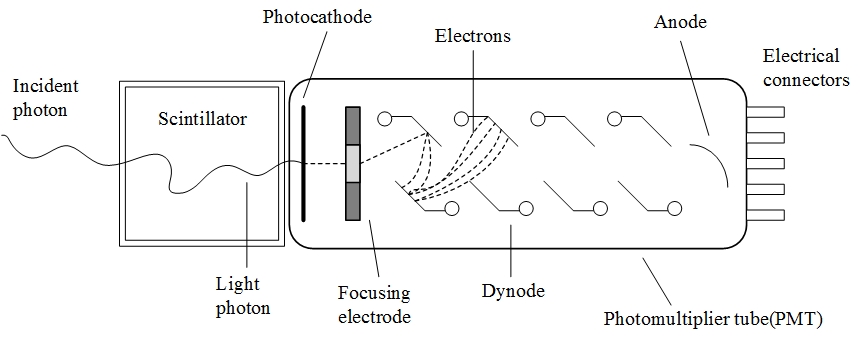
Scintillation detectors are employed to detect X-rays with energies higher than several keV. A scintillation detector is a combination of a crystal, which emits optical light photons when absorbing X-ray photons, and a light sensor, which collects the optical photons (Fioretti and Bulgarelli, 2020) (see Fig.15). The light sensors are typically Photo-Multiplier Tubes (PMT), photodiodes, silicon photo-multipliers, and SDD. In practice, a phoswich, a combination of two different crystals, is usually employed instead of a single crystal. The NaI(Tl)/CsI(Na) phoswich has been applied to RXTE (Rothschild et al., 1998) and Insight-HXMT (Liu et al., 2020).

Figure 15: Schematic diagram of a scintillation detector comprising a scintillation material coupled to a PMT

6.2.5 CdZnTe detector

Cadmium Telluride (CdTe) and Cadmium Zinc Telluride
(CdZnTe) detectors are semiconductor detectors with a function principle similar to SDDs. However, in CdZnTe detectors, the electrons collected in each pixel are read out independently (Arnaud et al., 2011). Nowadays, CdZnTe detectors become the modern standard instrument for detecting X-rays with energies above several keV, and have been applied to Swift and NuSTAR.

7 Pulse TOA estimation

Given the large distance and so the low X-ray flux of a pulsar, a pulsar cannot be detected to have regularly distributed pulses like a beacon. In this case, a spacecraft can only record a series of events within an exposure, which lasts from $t_{0}$ to $t_{\mathrm{f}}$, on a pulsar Emadzadeh and Speyer (2010). It should be noted that an event indicates not only the arrival of an X-ray photon from the pulsar but also possibly the arrival of the background, which could come from CXB, space particles and the nebula surrounding the pulsar.

When there are $M$ events recorded, the events can be denoted as $\{t_{i}\}_{i=1}^{M}$ with $t_{i}$ denoting the arrival time of the $i$th event. As a consequence, the pulse TOA estimation is to estimate the pulse TOA at $t_{0}$ or at $t_{\mathrm{f}}$ out of $\{t_{i}\}_{i=1}^{M}$. In most cases, the pulse TOA estimation is accomplished by estimating the pulse phase.

7.1 Pulsar signal model

Given that $t_{i}$ denotes the $i$th event between $\left[t_{0},t_{\mathrm{f}}\right)$ and that the event indicates the arrival of X-ray photon or the background, each event follows a Poisson distribution (Ross, 2014). As a consequence, $\{t_{i}\}_{i=1}^{M}$ is a nonhomogeneous Poisson process (NHPP) with a time-varying rate $\lambda(t)\geq 0$ Emadzadeh and Speyer (2010). $\{t_{i}\}_{i=1}^{M}$ indicates there are $M$ events between $\left(t_{0},t_{\mathrm{f}}\right)$, and thus, $M$ is also a Poisson random variable with a probability of Emadzadeh and Speyer (2010)

$$P\left(M\right)=\frac{\left(\int_{t_{0}}^{t_{\mathrm{f}}}\lambda(\xi)\mathrm{d}\xi\right)^{M}\exp\left(-\int_{t_{0}}^{t_{\mathrm{f}}}\lambda(\xi)\mathrm{d}\xi\right)}{M!}$$ (7)

$\lambda(t)$ can be expressed as

$$\lambda(t)=\alpha h\left(\phi_{\mathrm{det}}(t)\right)+\beta\quad\mathrm{counts/s}$$ (8)

where $h\left(\phi\right)$ is the periodic pulse profile or template, $\phi_{\mathrm{det}}(t)$ is the detected phase, $\alpha$ and $\beta$ are the known pulsed count rate and background count rate, respectively, and counts/s denotes "counts per second".

Assuming the spacecraft is performing a linear uniform motion towards the pulsar or being stationary, $\phi_{\mathrm{det}}(t)$ in Eq.(8) is expressed as

$$\phi_{\mathrm{det}}(t)=\phi_{0}+f_{0}\left(t-t_{0}\right)$$ (9)

where $\phi_{0}$ is the pulse phase at $t_{0}$ and $f_{0}$ is the frequency of the detected pulsar signal. If the spacecraft is stationary, $f_{0}=F_{0}$. When the spacecraft moves towards the pulsar along a line, $f_{0}$ becomes

$$f_{0}=\left(1+\frac{v}{c}\right)F_{0}$$ (10)

where $v$ is the velocity of spacecraft along the spacecraft-pulsar line.

Taking the SEXTANT program as an example, Fig.1 shows the pulse profiles of six pulsars, and Table 4 provides $\alpha$ and $\beta$ of the pulsars selected by the program. As shown in Table 4, the background count rates of all pulsars are at least one order of magnitude higher than the pulsed count rates. Although the Crab pulsar has the highest pulsed count rate among the pulsars, its background count rate is still two orders of magnitude higher than its pulsed count rate. It indicates that all the X-ray pulsars are very faint sources. Moreover, the arrival of photons or background is random, which indicates that the pulse phase estimation belongs to the stochastic signal processing.

Table 4: Pulsed count rates ($\alpha$) and background count rates ($\beta$) of pulsars selected by SEXTANT program(Ray et al., 2017)

Pulsar	$\alpha\quad(\mathrm{cnts/s})$	$\beta\quad(\mathrm{cnts/s})$
PSR B1937+21	0.029	0.24
PSR B1821-24	0.093	0.22
PSR J0218+4232	0.082	0.20
PSR J0030+0451	0.193	0.20
PSR J1012+5307	0.046	0.20
PSR J0437-4715	0.283	0.62
PSR J2124-3358	0.074	0.20
PSR J0751+1807	0.025	0.20
PSR J1024-0719	0.015	0.20
PSR J2214+3000	0.029	0.26
Crab pulsar	660.000	13860.20

7.2 Basic pulse phase estimation frames

The basic pulse phase estimation problem is to estimate $\phi_{0}$ in Eq.(9) under the assumption that the spacecraft is performing a uniform linear motion toward the pulsar or stationary and that the evolution of spin frequency of pulsar is ignored.

This section introduces the current methods to solve the above problem. These methods can be divided into two classes: (A) estimating $\phi_{0}$ using epoch folding, and (B) estimating $\phi_{0}$ with the direct use of $\{t_{i}\}_{i=1}^{M}$.

7.2.1 Pulse phase estimation using epoch folding

(1) Estimation with known $f_{0}$

When $f_{0}$ in Eq.(9) is already known, the period of pulsar signal equals to $P=1/f_{0}$ and an empirical profile can be recovered from $\{t_{i}\}_{i=1}^{M}$. This recovery method is called epoch folding.

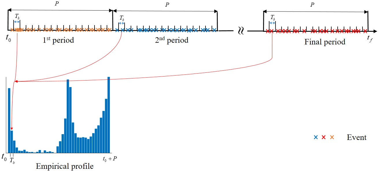
Assuming the exposure $\left[t_{0},t_{f}\right)$ contains $N$ periods, the epoch folding consists of three steps: (A) dividing the $i$th ($i=1,2,\cdots,N$) period into $N_{b}$ bins, each lasting for $T_{b}=P/N_{b}$; (B) the events falling in the $j$th bin of the latter periods are folded back into the $j$th bin of the first period (see Fig.16); (C) the event counts in each bin are normalized. Finally, an empirical profile is recovered. The statistical properties of the empirical profile have been investigated in Ref.123. It should be noted that the epoch folding is applied not only to XNAV but also to X-ray pulsar astronomy (Kirsch, M. G. F. et al., 2006; Martin-Carrillo, A. et al., 2012). This paper focuses on the application of epoch folding on XNAV.

Figure 16: Epoch folding procedure of a pulsar

The phase offset between the recovered empirical profile and the template is called $\phi_{0}$. Thus, the estimation of $\phi_{0}$ can be recast as the classical problem of estimating phase delay between two waveforms. The classical methods to estimate $\phi_{0}$ are cross-correlation (Emadzadeh and Speyer, 2011) and Nonlinear Least Square (NLS) (Emadzadeh and Speyer, 2010). The Cramer-Rao Low Bounds (CRLBs) for the $\phi_{0}$s estimated by cross-correlation and NLS are derived in Refs.123; 47.

Motivated by Refs.123; 47, many works started to pursue the fast computation, which is typically accomplished by Fast Fourier Transformation (FFT). For an empirical profile with $N_{b}$ bins, the computational complexity of cross-relation (Lin and Xu, 2019) with the aid of FFT is about $\mathcal{O}\left(N_{b}\log_{N_{b}}\right)$, much less than NLS (about $\mathcal{O}\left(N_{b}^{2}\right)$). FFT is also utilized by Refs.128 and 129, the bispectrum with the aid of FFT is applied in Ref.130, and the Discrete Fourier Transformation (DFT) is employed by Ref.131.

(2) Estimation with unknown $f_{0}$

When $f_{0}$ in Eq.(9) is unknown, we should first estimate $f_{0}$ and then estimate $\phi_{0}$ with the methods discussed above.

The estimation of $f_{0}$ is commonly solved by finding the period of a pulsar. Table 5(Lomb, 1976; Scargle, 1982; VanderPlas, 2018; Zechmeister and Kürster, 2009; Huijse et al., 2012; Schwarzenberg-Czerny, 1989, 1996; Stellingwerf, 1978; Palmer, 2009; Dworetsky, 1983; Graham et al., 2013a; Liu et al., 2019, 2020) lists the current period finding algorithms, in which the Lomb–Scargle, Generalized Lomb–Scargle and Correntropy kernel periodogram find the period in the frequency domain, and the other algorithms belong to time-domain methods. Although those methods are derived from different principles, they are dependent on the quality of the light curve of the pulsar. When the exposure on the pulsar is short and the pulsar has a faint magnitude, the quality of the final light curve is low and all those methods become inefficient (Graham et al., 2013b).

Table 5: Current period finding algorithms

Categroy	Algorithm
Astronomy	Lomb–Scargle(Lomb, 1976; Scargle, 1982; VanderPlas, 2018)
	Generalized Lomb–Scargle(Zechmeister and Kürster, 2009)
	Correntropy kernel periodogram(Huijse et al., 2012)
	Binned analysis of variance(Schwarzenberg-Czerny, 1989)
	Multiharmonic analysis of variance(Schwarzenberg-Czerny, 1996)
	Phase dispersion minimization(Stellingwerf, 1978)
	FastChi(Palmer, 2009)
	String length(Dworetsky, 1983)
	Conditional entropy(Graham et al., 2013a)
XNAV	Compressive sensing-based method(Liu et al., 2019)
	Fast butterfly epoch folding-based method(Liu et al., 2020)

7.2.2 Pulse phase estimation with direct use of events

When $f_{0}$ in Eq.(9) is known, according to Eqs.(7)-(9), the $M$-dimensional joint probability density of $\{t_{i}\}_{i=1}^{M}$ is (Emadzadeh and Speyer, 2010)

$$p\left(\left\{t_{i}\right\}_{i=1}^{M},\phi_{0}\right)=\mathrm{exp}\left(-\int_{t_{0}}^{t_{f}}\lambda(\tau;\phi_{0})\mathrm{d}\tau\right)\prod_{i=1}^{M}\lambda\left(t_{i};\phi_{0}\right)$$ (11)

Eq.(11) can be recognized as the likelihood function, and the Log-Likelihood Function (LLF) is

$$\operatorname{LLF}\left(\phi_{0}\right)=\sum_{i=1}^{M}\ln\left(\lambda\left(t_{i};\phi_{0}\right)\right)-\int_{t_{0}}^{t_{f}}\lambda(\tau;\phi_{0})\mathrm{d}\tau$$ (12)

The Maximum Likelihood Estimator (MLE) is provided by maximizing Eq.(12) with respect to the unknown $\phi_{0}$. The second term on the right side of Eq.(12) is not sensitive to $\phi_{0}$. As a consequence, the estimate of $\phi_{0}$, $\hat{\phi}_{0}$, can be expressed as

$$\hat{\phi}_{0}=\underset{\phi_{0}\in(0,1)}{\arg\max}\sum_{i=1}^{M}\ln\left(\lambda\left(t_{i};\phi_{0}\right)\right)$$ (13)

where $\arg\max\left(\bullet\right)$ denotes the argument of the maximum of the function within $\left(\bullet\right)$.

If $f_{0}$ in Eq.(9) is unknown, the right side of Eq.(12) can be viewed as a function of $\phi_{0}$ and $f_{0}$. Then, $\phi_{0}$ and $f_{0}$ can be estimated simultaneously by maximizing Eq.(12). In this case, we have

$$\hat{\phi}_{0},\hat{f}_{0}=\arg\max\sum_{i=1}^{M}\ln\left(\lambda\left(t_{i};\phi_{0},f_{0}\right)\right)$$ (14)

As shown in Eq.(14), MLE provides a more flexible frame to estimate $\phi_{0}$ and $f_{0}$ than the epoch folding method. In other words, if the evolution of spin frequency is taken into consideration, MLE can also work well, and can provide a result closer to the CRLB than NLS (Emadzadeh and Speyer, 2010).

Eq.(14) is usually solved by a two-dimensional grid search. When the grid for search is $N_{\phi}\times N_{f}$, the computational complexity of the MLE is about $\mathcal{O}\left(N_{\phi}\times N_{f}\times M\right)$, which is much higher than the computational complexity of NLS even when $N_{b}=N_{\phi}=N_{f}$. In order to accelerate the computation of Eq.(14), the intelligent optimization method is employed(Wang et al., 2021). However, the intelligent optimization method that utilizes the technique of random numbers cannot have a stable estimation result (Wang et al., 2021).

7.3 On-orbit pulse phase estimation

The methods introduced in Section 7.2 are based on the assumptions that the spacecraft is stationary or performs a linear uniform motion towards the pulsar. However, in practice, spacecraft orbit around a central celestial body, such as the Earth for the Earth-orbiting satellites or the Sun for deep space spacecraft (Battin, 1999). In this case, $f_{0}$ in Eq.(9) is time-varying and unknown, and then, Eq.(9) can be rewritten as (Golshan and Sheikh, 2007)

$$\phi_{\mathrm{det}}(t)=\theta_{0}+\int_{t_{0}}^{t}f\left(\tau\right)\mathrm{d}\tau\equiv\theta_{0}+\theta(t)$$ (15)

where

$$\theta(t)=f_{\mathrm{s}}\left(t-t_{0}\right)+\underbrace{\int_{t_{0}}^{t}f_{\mathrm{d}}\left(\tau\right)\mathrm{d}\tau}_{\equiv\theta_{\mathrm{d}}(t)}$$ (16)

where $f_{\mathrm{s}}$ is the spin frequency of the pulsar and $\theta_{\mathrm{d}}(t)$ is the phase caused by the Doppler frequency.

In this case, there are currently two frames for estimating the pulse phase: (A) pulse phase tracking and (B) estimation with linearized pulse phase model.

7.3.1 Pulse phase tracking

The pulse phase tracking algorithm, which consists of a MLE followed by a Digital Phase-Locked Loop (DPLL), was first proposed in Ref.148. The main idea, illustrated in Fig.17, is to partition the whole exposure into $N$ blocks and the detected signal frequency is approximately constant over each block. Events obtained over the $i$th block are processed by the two-dimensional MLE shown in Eq.(14). In order to reduce the estimation errors or noise in the MLE output sequence, the MLE output sequence is smoothed by the DPLL (Stephens and Thomas, 1995).

Figure 17: Diagram illustrating the pulse phase tracking concept

Ref.150 verified the pulse phase tracking algorithm in three cases where the simulated trajectories were all one-dimensional, and relaxed the constant signal frequency assumption using a MLE with a second-order Taylor polynomial phase model and feedback of frequency and its first derivative using a third-order digital phase-locked loop(Anderson et al., 2022). It is found that the phase tracking has a great promise for deep space navigation, but only more limited potential in scenarios where the orbital dynamics is high and the faint MSPs are observed for navigation.

7.3.2 Pulse estimation with linearized pulse phase model

As illustrated in Ref.151, the phase tracking algorithm limits its potential in the environment with high orbital dynamics such as the Earth space. However, the current flight experiments on XNAV have to be performed on an Earth-orbiting spacecraft. In this case, the pulse estimation with linearized pulse phase model was proposed (Winternitz et al., 2016, 2018; Wang and Zheng, 2016; Wang and Zhang, 2016).

It follows from Eq.(3) that Eq.(2) can be recognized as a function of $\bm{r}_{\mathrm{SSB}}(t)$. In practice, we can have a prior information on $\bm{r}_{\mathrm{SSB}}(t)$, denoted as $\tilde{\bm{r}}_{\mathrm{SSB}}(t)$. Then, Eq.(2) can be linearized around $\tilde{\bm{r}}_{\mathrm{SSB}}(t)$, yielding

$$\left\{\begin{aligned} &\phi\left(\bm{r}_{\mathrm{SSB}}(t)\right)=\phi\left(\tilde{\bm{r}}_{\mathrm{SSB}}(t)\right)+\left.\frac{\partial\phi}{\partial\bm{r}}\right|_{\bm{r}=\tilde{\bm{r}}_{\mathrm{SSB}}(t)}\delta\bm{r}_{\mathrm{SSB}}(t)\\ &\delta\bm{r}_{\mathrm{SSB}}(t)=\bm{r}_{\mathrm{SSB}}(t)-\tilde{\bm{r}}_{\mathrm{SSB}}(t)\end{aligned}\right.$$ (17)

$\tilde{\bm{r}}_{\mathrm{SSB}}(t)$ can be predicted from $\tilde{\bm{r}}_{\mathrm{SSB}}(t_{0})$, obtained by other navigation methods or by propagating from the last epoch, by propagating the orbit dynamics model of spacecraft (Battin, 1999). As a consequence, $\phi\left(\bm{r}_{\mathrm{SSB}}(t)\right)$ can be expressed as (Winternitz et al., 2016, 2018)

$$\phi\left(\bm{r}_{\mathrm{SSB}}(t)\right)=\phi\left(\tilde{\bm{r}}_{\mathrm{SSB}}(t)\right)+\phi_{0}+f_{\mathrm{a}}\left(t-t_{0}\right)$$ (18)

where $\phi_{0}$ and $f_{\mathrm{a}}$ are unknown.

Given that the events set $\{t_{i}\}_{i=1}^{M}$ follows a Poisson process,
$\{\phi\left(\bm{r}_{\mathrm{SSB}}(t_{i})\right)\}_{i=1}^{M}$ also follows a Poisson process with constant $\phi_{0}$ and $f_{\mathrm{a}}$. Thus, $\phi_{0}$ and $f_{\mathrm{a}}$ can be estimated by solving a two-dimensional optimization problem:

$$\hat{\phi}_{0},\hat{f}_{\mathrm{a}}=\arg\max\sum_{i=1}^{M}\ln\left(\lambda\left(\phi_{0},f_{\mathrm{a}},\tilde{\bm{r}}_{\mathrm{SSB}}(t_{i})\right)\right)$$ (19)

The SEXTANT team employs the two-dimensional grid search to solve the above problem (Winternitz et al., 2016). In order to reduce the computational complexity, the parallel computation is employed to accelerate the grid search (Wang and Zheng, 2016), and decouples the estimation of $\phi_{0}$ and $f_{\mathrm{a}}$ for deep space exploration missions (Wang and Zhang, 2016). $f_{\mathrm{a}}$ is first searched out and then $\phi_{0}$ is estimated by epoch folding. Recently, an on-orbit pulsar timing analysis is proposed to fast estimate $\phi_{0}$, and has been verified by the data from XNAV flight experiments(Wang et al., 2022).

8 Methods to improve the navigation performance of XNAV

The principle of XNAV was briefly summarized in Section 4. We first need to find an optimal pulsar combination from a given navigation pulsar database. When the optimal pulsar combination is achieved, both the geometry for a specific navigation mission and the corresponding navigation performance of XNAV in this case can be improved. Moreover, there are many systematic biases within XNAV, which limit the navigation performance of XNAV. Furthermore, the conventional XNAV works with the assumption that a single spacecraft should load at least three X-ray detection systems with large areas to receive the pulsar signal from three directions. This assumption is too ideal for the practical applications. Therefore, in order to improve the navigation performance of XNAV, this section will introduce three types of methods.

8.1 Optimal pulsar combination

This work is usually accomplished by investigating the observability of the navigation system. Most time, the observability is evaluated by the determinant of Fisher Information Matrix (FIM). When there are three pulsars being observed simultaneously, the FIM is derived as (Wang et al., 2017a)

$$\bm{F}=\sum_{i=1}^{3}\sigma_{i}^{-2}\bm{n}_{i}\bm{n}_{i}^{\mathrm{T}}$$ (20)

where $\bm{n}_{i}$ is the direction vector of the $i$th pulsar and $\sigma_{i}$ is the accuracy of the $i$th pulse TOA.

Based on Eq.(20), Ref.158 analytically investigates the optimal pulsar combination, and find that the determinant of Eq.(20) will reach its maximum if $\bm{n}_{1}$, $\bm{n}_{2}$ and $\bm{n}_{3}$ are orthogonal to each other. This conclusion can be extended to a general case where a spacecraft observes $N$ pulsars at the same time. In this case, an optimal pulsar combination should be composed of pulsars with direction vectors orthogonal to each other.

8.2 Systematic biases analysis and compensation

As shown in Eq.(3), the errors within the direction vector of pulsar, positions of planets and the atomic clock recording arrival time of events would affect the navigation performance of XNAV.

For the autonomous navigation in Earth orbits, the impacts of errors within the direction vector of the pulsar, errors within the ephemerides of planets, and clock errors have been analyzed(Liu et al., 2010; Xu et al., 2018a; Wang et al., 2013a, 2014). It is found that those errors vary according to the orbit period of the Earth and thus can be approximated as constants for a navigation process with duration much less than one orbit period of the Earth. This conclusion paves the way for compensating the impacts of those errors. When the XNAV is applied to multi-spacecraft, it has been found that the systematic biases can be eliminated when all the spacecraft observe a common pulsar simultaneously (Xiong et al., 2009).

The compensation methods generally consist of three categories, including the augmented-state method (Liu et al., 2010), the time-differenced method (Wang et al., 2014, 2019) and the $H_{\infty}/H_{2}$ filter (Xiong et al., 2010). The augmented-state method augments the systematic biases into the state vector, and estimates the systematic biases along with the position and velocity of spacecraft. However, when the number of systematic biases is more than 6, the number of position and velocity, Kalman-type filters employed for estimation might be unstable. Thus, the time-differenced method was proposed. The method employs the difference between pulse TOAs at adjacent time as the measurement for estimation, avoiding the high-dimensional matrices that were involved in the augmented-state method. The $H_{\infty}/H_{2}$ filter, originating from the $H_{\infty}$ control, derives an upper bound for the systematic biases, and suppresses the impacts of systematic biases by the bounds. However, how to design a proper upper bound is still an open question.

8.3 Integrated navigation

Up to now, the information to be combined with XNAV roughly includes the Earth image information obtained from ultraviolet sensor (Qiao et al., 2009), the Doppler velocity measurements relative to the Sun (Wang et al., 2015) or the Mars (Cui et al., 2016), the optical measurements on the Mars (Liu et al., 2017; Gu et al., 2019) or the Earth (Wang et al., 2013b; Xiong et al., 2016), and the output of inertial navigation system (Xu et al., 2018b; Wang et al., 2016). For the integrated navigation system fusing the star angle information and XNAV, the impacts of direction vector of pulsar(Ning et al., 2017a), and the ephemerides errors of Jupiter and other planets(Ning et al., 2017b; Gui et al., 2019; Ning et al., 2018) have been investigated. The integrated navigation is applied not only to a single spacecraft but also to multi-spacecraft (Xin et al., 2018; Liu et al., 2015).

The fusion of information from other sources and XNAV is typically achieved by the federated Kalman filter. The federated Kalman filter consisting of parallel filters for each information fuses the outputs of the parallel filters to obtain the final estimation result. Given that the parallel filters work independently, the final estimation result is suboptimal (Wang et al., 2013b). A nonlinear kinematic and static filter is derived (Wang et al., 2013b, 2016) to overcome the suboptimal fusion of federated Kalman filter. A step Kalman filter structure is designed(Shang et al., 2013) to optimally fuse the parallel filters that have greatly different filtering precision. However, the above information fusions work by fusing the pulse phase or TOA and the measurements from the other sources. The achievements of such information fusions are based on the assumption that the pulse phase is obtained. However, as illustrated in Section 7.3, the on-orbit pulse TOA estimation problem has not been well solved. It is a good idea to employ the measurements from the other sources to estimate the pulse phase(Xiong et al., 2016; Wang et al., 2017b).

9 Conclusions and future work

In this paper, we review X-ray pulsar navigation (XNAV) systems and the algorithms, and briefly introduce the past, present and future missions with XNAV experiments. This paper focuses on the advances of the key techniques supporting XNAV, including the navigation pulsar database, the X-ray detection system, and the pulse TOA estimation, as well as the methods to improve the navigation performance of XNAV.

It can be learned from the review that although several flight experiments on XNAV have been successfully complemented, the wide applications of XNAV still have a long way to go. Further development of XNAV may be pursued from the following aspects:

1. Designing X-ray detection systems dedicated for navigation. The current X-ray detection systems in space, serve for X-ray astronomy missions, which pursue high-quality images or signals with high signal-to-noise ratios. In this case, the volume and weight of an X-ray detection system dominate the payload. However, for a spacecraft with XNAV, the X-ray detection system is just a subsystem of the whole spacecraft. As a consequence, an X-ray detection system dedicated for navigation should be of a small size but have a high detection performance.

2. Pursuing computationally efficient on-orbit pulse TOA estimation method. Currently, only the pulse TOA estimation for millisecond pulsars have been successfully complemented in orbit. The high flux of Crab pulsar makes the XNAV with small X-ray detection system become applicable, although the stability of Crab pulsar is far less than millisecond pulsars. However, how to quickly estimate the pulse TOA of the Crab pulsar in orbit is an open question. It is because the computational burden in this case is much higher than millisecond pulsars.

3. Verifying the current navigation algorithms with real X-ray pulsar data. Section 8 reviews various navigation algorithms that have been proposed to improve the navigation performance of XNAV. However, most of those algorithms work with simulation data under the assumption that the high-precision pulse ToAs can be obtained. In the algorithms, X-ray detection systems are assumed to have an area of about 1 $\mathrm{m}^{2}$. However, as shown in Tables 2 and 3, such a big area is not easy to achieve in space, even for dedicated X-ray astronomical missions. Furthermore, the flux of a pulsar’s pulsed signal is much less than the background caused by the particles and X-rays from other sources. Thus, the pulse TOA estimation result in the real environment is less accurate than the values assumed in the navigation algorithms. As a consequence, the performance of those navigation algorithms in real cases is quite probably not as good as that in simulations.

References

- Becker et al. (2013) Becker W, Bernhardt MG, Jessner A. Autonomous spacecraft navigation with pulsars. Acta Futura 2013;7:1128.
- James et al. (2009) James N, Abello R, Lanucara M, et al. Implementation of an ESA delta-DOR capability. Acta Astronaut 2009;64(1112):10419.
- Williams (2002) Williams B. Technical challenges and results for navigation of NEAR shoemaker. Johns Hopkins Apl Tech Dig 2002;23:3445.
- Mourikis et al. (2009) Mourikis AI, Trawny N, Roumeliotis SI, et al. Vision-aided inertial navigation for spacecraft entry, descent, and landing. IEEE Trans Robotics 2009;25(2):26480.
- Amzajerdian et al. (2011) Amzajerdian F, Pierrottet D, Petway L, et al. Lidar systems for precision navigation and safe landing on planetary bodies. International symposium on photoelectronic detection and imaging 2011:Laser sensing and imaging; and biological and medical applications of photonics sensing and imaging. Beijing, China. San Francisco: SPIE;2011:8192.
- Gaskell et al. (2008) Gaskell RW, Barnouin-Jha OS, Scheeres DJ, et al. Characterizing and navigating small bodies with imaging data. Meteorit Planet Sci 2008;43(6):104961.
- Wood (1993a) Wood KS. Navigation studies utilizing the NRL-801 experiment and the ARGOS satellite.. Optical engineering and photonics in aerospace sensing. Orlando, USA. San Francisco:SPIE;1993: 10516.
- Lorimer and Kramer (2004) Lorimer D, Kramer M. Handbook of pulsar astronomy. Cambridge: Cambridge University Press; 2004. p. 20038.
- Hewish et al. (1969) Hewish A, Bell SJ, Pilkington JDH, et al. Observation of a rapidly pulsating radio source. Nature 1968;217(5130):70913.
- Lattimer and Prakash (2004) Lattimer JM, Prakash M. The physics of neutron stars. Science 2004;304(5670):53642.
- Kohlhase and Penzo (1977) Kohlhase CE, Penzo PA. Voyager mission description. Space Sci Rev 1977;21(2):77101.
- Sagan et al. (1972) Sagan C, Sagan LS, Drake F. A message from earth. Science 1972;175(4024):8814.
- Ghosh (2007) Ghosh P. Rotation and accretion powered pulsars. Singapore: World Scientific; 2007. p.134.
- Rawley et al. (1987) Rawley LA, Taylor JH, Davis MM, et al. Millisecond pulsar PSR 1937+21:A highly stable clock. Science 1987;238(4828):7615.
- Hartnett and Luiten (2011) Hartnett JG, Luiten AN. Colloquium: Comparison of astrophysical and terrestrial frequency standards. Rev Mod Phys 2011;83(1):19.
- (16) Mitchell JW, Hassouneh M, Winternitz L, et al. SEXTANT - Station Explorer for X-ray Timing and Navigation Technology. Reston: AIAA; 2015. Report No.: AIAA-2015-0865.
- Hintz (2015) Hintz G. Orbital mechanics and astrodynamics: Techniques and tools for space missions. Berlin: Springer; 2015. p. 1386.
- IAU SOFA Center (2014) iausofa.org [Internet]. New York: international astronomical union; c2001-21 [updated 2021 May 11; cited 2022 Sept 28]. Available from: http://iausofa.org/.
- Downs (1974) Downs G. Interplanetary navigation using pulsating radio sources. Jet propulsion lab: US; 1974. Report No.: JPL-TR-32-1594.
- Chester and Butman (1981) Chester T, Butman S. Navigation using X-ray pulsars. Washington, D.C.: NASA; 1981. Report No.: NASA-19810018585.
- Ray et al. (2001) Ray PS, Wood KS, Fritz G, et al. The USA X-ray timing experiment. AIP Conf Proc 2001;599(1):33645.
- Kowalski et al. (2001) Kowalski M, Wood D, Fritz G, et al. The unconventional stellar aspect (USA) experiment on ARGOS. Reston: AIAA; 2001. Report No.:AIAA-2001-4664.
- Wood and Ray (2017) Wood KS, Ray PS. [Internet] The NRL program in X-ray navigation.[updated 2011 Dec 11, cited 2022 Sept 28]. Availiable from https://arxiv.org/abs/1712.03832.
- Beckett (2006) Beckett D. Overview of the XNAV program, X-ray navigation using celestial sources. Broomfield: Ball Corporation; 2006. Report No.:SSC06-VI-6.
- Sheikh et al. (2011) Sheikh SI, Hanson JE, Graven PH, et al. Spacecraft navigation and timing using X-ray pulsars. Navigation 2011;58(2):16586.
- Gendreau et al. (2012) Gendreau KC, Arzoumanian Z, Okajima T. The Neutron star Interior Composition ExploreR (NICER): An explorer mission of opportunity for soft X-ray timing spectroscopy. SPIE astronomical telescopes instrumentation. Amsterdam, Netherlands. San Francisco: SPIE; 2012: 3229.
- Mitchell et al. (2014) Mitchell JW, Hassouneh MA, Winternitz LM, et al. Station explorer for X-ray timing and navigation technology architecture overview. Proceedings of the 27th international technical meeting of the satellite division of the institute of bavigation (ION GNSS+). Manassas: Institute of navigation; 2014. p. 3194200.
- Witze (2018) Witze A. NASA test proves pulsars can function as a celestial GPS. Nature 2018;553(7688):2612.
- Piriz et al. (2019) Piriz R, Garbin E, Roldan P, et al. PulChron: A pulsar time scale demonstration for PNT systems.Proceedings of the 50th Annual Precise Time and Time Interval Systems and Applications Meeting. Manassas: Institute of navigation; 2019. p. 191205.
- Garbin et al. (2019) Garbin E, Piriz R, Binda S, et al. PULCHRON: A live pulsar time scale demonstration. 14th Meeting of the international committee on global navigation satellite systems Bengaluru: Indian Space Research organization; 2019. p. 113.
- Ferdman et al. (2010) Ferdman RD, van Haasteren R, Bassa CG, et al. The european pulsar timing array: Current efforts and a LEAP toward the future. Class Quantum Grav 2010;27(8):084014.
- Zhang et al. (2017) Zhang XY, Shuai P, Huang LW, et al. Mission overview and initial observation results of the X-ray pulsar navigation-I satellite. Int J Aerosp Eng 2017;2017:17.
- Huang et al. (2019) Huang LW, Shuai P, Zhang XY, et al. Pulsar-based navigation results: data processing of the X-ray pulsar navigation-I telescope.Journal of Astronomical Telescopes, Instruments, and Systems 2019;5(1):18.
- Huang et al. (2017) Huang L, Zhang X, Du Y, et al. The largest glitch of the Crab pulsar detected at the X-ray band. The Astronomer’s Telegram 2017;11025:1.
- Zheng et al. (2017) Zheng SJ, Ge MY, Han DW, et al. Test of pulsar navigation with POLAR on TG-2 space station. Sci Sin-Phys Mech Astron 2017;47(9):099505 [Chinese].
- Zhang et al. (2020) Zhang SN, Li TP, Lu FJ, et al. Overview to the hard X-ray modulation telescope (Insight-HXMT) satellite. Sci China Phys Mech Astron 2020;63(4):249502.
- Zheng et al. (2019) Zheng SJ, Zhang SN, Lu FJ, et al. In-orbit demonstration of X-ray pulsar navigation with the Insight-HXMT satellite. Astrophys. J., Suppl. Ser., 2019; 244:17.
- Sun et al. (2022) Sun HF, Su JY, Deng ZW, et al. Grouping bi-chi-squared method for pulsar navigation experiment using observations of Rossi X-ray timing explorer. Chin J Aeronaut 2023;36(1):38695.
- Romaine et al. (2018) Romaine S, Kraft R, Gendreau K, et al. CubeSat X-ray telescope (CubeX) for lunar elemental abundance mapping and millisecond X-ray pulsar navigation. Logan: Utah State University, UT; 2018. Report No.:SSC18-V-05.
- Kandala et al. (2021) Kandala A, Oza A, Saiguhan B, et al. Mission concept for demonstrating small-spacecraft true anomaly estimation using millisecond X-Ray pulsars; Logan: Utah State University, UT; 2021. Report No.:SSC21-VI-08.
- Alam et al. (2021) Alam MF, Arzoumanian Z, Baker PT, et al. The NANOGrav 12.5 yr data set: observations and narrowband timing of 47 millisecond pulsars. Astrophys J Suppl Ser 2020;252(1):4.
- Lyne et al. (1993) Lyne AG, Pritchard RS, Graham Smith F. 23 years of Crab pulsar rotational history. Mon Not R Astron Soc 1993;265(4):100312.
- Rea (2017) Rea ND. Fifty years of pulsar astrophysics. Nat Astron 2017;1(12):82930.
- Edwards et al. (2006) Edwards RT, Hobbs GB, Manchester RN. Tempo2, a new pulsar timing package - II. The timing model and precision estimates. Mon Not R Astron Soc 2006;372(4):154974.
- Buist et al. (2011) Buist PJ, Engelen S, Noroozi A, et al. Overview of pulsar navigation: Past, present and future trends. Navigation 2011;58(2):15364.
- Zheng and Wang (2020) Zheng W, Wang YD. X-ray pulsar-based navigation: Theory and applications. Singapore: Springer Singapore, 2020; p.1-200.
- Emadzadeh and Speyer (2011) Emadzadeh AA, Speyer JL. X-ray pulsar-based relative navigation using epoch folding. IEEE Trans Aerosp Electron Syst 2011;47(4):231728.
- Xiong et al. (2009) Xiong K, Wei CL, Liu LD. The use of X-ray pulsars for aiding navigation of satellites in constellations. Acta Astronaut 2009;64(4):42736.
- Manchester et al. (2005) Manchester RN, Hobbs GB, Teoh A, et al. The Australia telescope national facility pulsar catalogue. Astron J 2005;129(4):19932006.
- Becker (2009) Becker W. X-Ray Emission from Pulsars and Neutron Stars. Neutron Stars and Pulsars. Berlin: Springer, 2009. p.91140.
- Taylor (1991) Taylor JH. Millisecond pulsars: Nature’s most stable clocks. Proc IEEE 1991;79(7):105462.
- Matsakis et al. (1997) Matsakis DN, Taylor JH,. A statistic for describing pulsar and clock stabilities. Astron Astrophys 1997;326(3):9248.
- Shaw et al. (2018) Shaw B, Lyne AG, Stappers BW, et al. The largest glitch observed in the Crab pulsar. Mon Not R Astron Soc 2018;478(3):383240.
- McLaughlin (2013) McLaughlin MA. The North American nanohertz observatory for gravitational waves. Class Quantum Grav 2013;30(22):224008.
- Ray et al. (2017) Ray PS, Wood KS, Wolff MT. [Internet] Characterization of pulsar sources for X-ray navigation. [updated 2017 Nov 22; cited 2022 Sept 28]. Availiable from https://arxiv.org/abs/1711.08507
- Reardon et al. (2016) Reardon DJ, Hobbs G, Coles W, et al. Timing analysis for 20 millisecond pulsars in the Parkes pulsar timing array. Mon Not R Astron Soc 2016;455(2):175169.
- Sheikh et al. (2006) Sheikh SI, Pines DJ, Ray PS, et al. Spacecraft navigation using X-ray pulsars. J Guid Control Dyn 2006;29(1):4963.
- Kalemci (2018) Kalemci E. Summary of the past, present and future of the X-ray astronomy. Eur Phys J Plus 2018;133(10):407.
- Ramsey et al. (1993) Ramsey BD, Austin RA, Decher R. Instrumentation for X-ray astronomy. Space Sci Rev 1994;69(1):139204.
- Fabian (1975) Fabian AC. UHURU - the first X-ray astronomy satellite. Journal of the British Interplanetary Society 1975;28:3436.
- Giacconi et al. (1971) Giacconi R, Kellogg E, Gorenstein P, et al. An X-ray scan of the galactic plane from UHURU. The Astrophysical Journal 1971;165:L27.
- Sanford (1974) Sanford PW. X-ray observations of variable sources. Proc R Soc Lond A 1974;340(1623):41122.
- Gursky et al. (1978) Gursky H, Bradt H, Doxsey R, et al. Measurements of X-ray source positions by the scanning modulation collimator on HEAO 1. The Astrophysical Journal 1978;223: 973.
- Rothschild et al. (1979) Rothschild R, Boldt E, Holt S, et al. The Cosmic X-ray Experiment Aboard HEAO-1. Space Science Instrumentation 1979;4:269301.
- Turner et al. (1981) Turner ML, Smith A, Zimmermann HU. The medium energy instrument on exosat. Space Sci Rev 1981;30(1):51324.
- Turner et al. (1989) Turner MJL, Thomas HD, Patchett BE, et al. The large area counter on Ginga. Publications of the Astronomical Society of Japan 1989;41:34572.
- Jahoda et al. (2006) Jahoda K, Markwardt CB, Radeva Y, et al. Calibration of the Rossi X-ray timing explorer proportional counter array. Astrophys J Lett Suppl Ser 2006;163(2):40123.
- Bradt et al. (1968) Bradt H, Garmire G, Oda M, et al. The modulation collimator in X-ray astronomy. Space Sci Rev 1968;8(4):471506.
- Smith and Courtier (1976) Smith JF, Courtier GM. The Ariel 5 Programme. Proceedings of the Royal Society of London Series A 1976;350(1663):42139.
- Smith (2006) Smith RK. The Chandra X-ray observatory: An astronomical facility available to the world. Astrophys Space Sci 2006;305(3):3214.
- Ade et al. (2022) Ade PAR, Matthew J G, Tucker CE. X-ray, -ray, and astro-particle detection. Physical Principles of Astronomical Instrumentation. Boca Raton: CRC Press; 2021. p.25390.
- O’Dell et al. (2010) O’dell SL, Brissenden RJ, Davis WN, et al. High-resolution X-ray telescopes. SPIE optical engineering + applications, adaptive X-ray optics. San Francisco: SPIE; 2010:120.
- Gorenstein P (2012) Gorenstein P. Grazing incidence telescopes for X-ray astronomy. Opt Eng 2012;51(1): 011010.
- Tousey (1977) Tousey R. Apollo telescope mount of skylab: An overview. Appl Opt 1977;16(4):82536.
- Giacconi et al. (1979) Giacconi R, Branduardi G, Briel U, et al. The Einstein/HEAO 2/X-ray observatory. The Astrophysical Journal 1979;230: 54054050.
- Taylor et al. (1981) Taylor BG, Andresen RD, Peacock A, et al. The exosat mission. Space Sci Rev 1981;30(1-4):47994.
- Korte et al. (1981) de Korte PAJ, Bleeker JM, den Boggende AJF, et al. The X-ray imaging telescopes on exosat. Space Sci Rev 1981;30(1):495511.
- Aschenbach (1988) Aschenbach B. Design, construction, and performance of the ROSAT highresolution X-ray mirror assembly. Appl Opt 1988;27(8):140413.
- Serlemitsos et al. (1995) Serlemitsos PJ, Jalota L, Soong Y, et al. The X-ray telescope on board ASCA. Publications of the Astronomical Society of Japan 1995;47:10514.
- Gorenstein (2010) Gorenstein P. Focusing X-ray optics for astronomy. X-Ray Opt Instrum 2010;2010: 109740.
- Lumb et al. (2012) Lumb DH, Jansen FA, Schartel N. X-ray multi-mirror mission (XMM-Newton) observatory. Opt Eng 2012;51(1):011009.
- Burrows et al. (2005) Burrows DN, Hill JE, Nousek JA, et al. The swift X-ray telescope. Space Science Reviews 2005;120(34):16595.
- Serlemitsos et al. (2007) Serlemitsos PJ, Soong Y, Chan KW, et al. The X-ray telescope onboard suzaku. Publ Astron Soc Jpn Nihon Tenmon Gakkai 2007;59(sp1):S9S21.
- Harrison et al. (2013) Harrison FA, Craig WW, Christensen FE, et al. The Nuclear Spectroscopic Telescope array (NuSTAR) high-energy X-ray mission. The Astrophysical Journal 2013;770(2):103.
- Singh et al. (2014) Singh KP, Tandon SN, Agrawal PC, et al. ASTROSAT mission. Space Telescopes and Instrumentation 2014: Ultraviolet to Gamma Ray. San Francisco: SPIE; 2014: 91441S.
- Takahashi et al. (2018) Takahashi T, Kokubun M, Mitsuda K, et al. Hitomi (ASTRO-H) X-ray astronomy satellite. J Astron Telesc Instrum Syst 2018;4(2):1.
- Sato et al. (2016) Sato T, Iizuka R, Ishida M, et al. Examining the angular resolution of the ASTRO-H’s soft X-ray telescopes. 2016; 2(4):111.
- Li et al. (2018) Li LS. Assembly error analysis and In-orbit verification of grazing incidence focusing X-ray pulsar telescope. J Mech Eng 2018;54(11):4960 [Chinese].
- Okajima et al. (2016) Okajima T, Soong Y, Balsamo ER, et al. Performance of NICER flight X-ray concentrator. SPIE Astronomical Telescopes + Instrumentation. San Francisco:SPIE; 2016: 1495501.
- Friedrich et al. (2008) Friedrich P, Bräuninger H, Budau B, et al. Design and development of the eROSITA X-ray mirrors. SPIE Astronomical Telescopes+Instrumentation. San Francisco:SPIE; 2016: 85360.
- Pavlinsky et al. (2021) Pavlinsky M, Tkachenko A, Levin V, et al. The ART-XC telescope on board the SRG observatory.. Astron Astrophys 2021;650: A42.
- Wolter (1952) Wolter H. Spiegelsysteme streifenden einfalls als abbildende optiken für röntgenstrahlen. Ann Phys 1952;445(12):94114 [German].
- Schmidt (1975) Schmidt WKH. A proposed X-ray focusing device with wide field of view for use in X-ray astronomy.. Nucl Instrum Methods 1975;127(2):28592.
- Angel (1979) Angel JRP. Lobster eyes as X-ray telescopes. The Astrophysical Journal 1979;223: 364.
- Pina et al. (2019) Pina L, Hudec R, Marsikova V, et al. X-ray multi-foil optical system for CubeSat demonstrator. SPIE optical engineering + applications.. San Francisco:SPIE; 2019: 11731.
- Gorenstein (1987) Gorenstein P. All Sky Supernova and Transient Explorer (ASTRE). In: Variability of Galactic and Extragalactic X-ray Sources;. Milano-Bologna: Treves Ed. Associazione per LAvanzamento dellAstronomia; 1987: 25363.
- Fraser et al. (2002) Fraser GW, Brunton AN, Bannister NP, et al. LOBSTER-ISS: An imaging X-ray all-sky monitor for the International Space Station.International symposium on optical science and technology.. San Francisco:SPIE; 2002: 11526.
- min Yuan et al. (2018) Yuan WM, Zhang C, Ling ZX, et al. Einstein Probe: a lobster-eye telescope for monitoring the X-ray sky.. SPIE astronomical telescopes + instrumentation. San Francisco:SPIE; 2018: 54351.
- Fraser et al. (2002) Fraser GW, Brunton AN, Bannister NP, et al. LOBSTER-ISS: an imaging X-ray all-sky monitor for the International Space Station. International symposium on optical science and technology. San Francisco:SPIE; 2002: 11526.
- Yuan et al. (2018a) Yuan W, Jin C, Zhang C, et al. The Einstein probe mission: A lobster-eye X-ray monitor for exploring the transient X-ray sky. 42nd COSPAR Scientific Assembly; California: California Institute of Technology; 2018: E1.174018.
- Yuan et al. (2018b) Yuan WM. Special topic of Einstein probe: exploring the dynamic X-ray universe.. Sci Sin-Phys Mech Astron 2018;48(3):039501 [Chinese].
- Götz et al. (2009) Götz D, Paul J, Basa S, et al. SVOM: A new mission for Gamma-Ray Burst Studies. AIP conference proceedings. Melville: AIP; 2009. p. 2530.
- Feldman et al. (2017) Feldman C, Pearson J, Willingale R, et al. Testing and modelling of the SVOM MXT narrow field lobster-eye telescope. Optics for EUV, X-Ray, and Gamma-ray astronomy VIII.. San Francisco:SPIE; 2017: 103991Q.
- Arnaud et al. (2011) Arnaud K, Smith R, Siemiginowska A. Handbook of X-ray Astronomy. Cambridge: Cambridge University Press; 2011. p. 2358.
- Xu and Brown (1987) Xu QZ, Brown LM. The early history of cosmic ray research.. Am J Phys1987;55(1):2333.
- Winkler et al. (2015) Winkler A, Karadzhinova A, Hildén T, et al. A gaseous proportional counter built from a conventional aluminum beverage can. Am J Phys 2015;83(8):73340.
- Conde and Policarpo (1967) Conde CAN, Policarpo AJPL. A gas proportional scintillation counter. Nucl Instrum Methods 1967;53: 712.
- White (1990) White NE. Astronomy with exosat.. Adv Space Res 1990;10(2):2140.
- Trümper and Hasinger (2008) Trümper JE, Hasinger G. Proportional counters. The universe in X-rays. Berlin: Springer; 2008. p.514.
- Fioretti and Bulgarelli (2020) Fioretti V, Bulgarelli A. Tutorial Guide to X-ray and -ray Astronomy. Singapore: Springer; 2020. p.55117.
- (111) Basic principles of image sensors [Internet]. The national thematic university; [updated 2002 May 16; cited 2022 Sept 28]. Available from: .
- Nakajima et al. (2009) Nakajima H, Matsuura D, Anabuki N, et al. Development of X-ray CCD camera system with high readout rate using ASIC. Nucl Instrum Methods Phys Res Sect A Accel Spectrometers Detect Assoc Equip 2009;610(1):7882.
- Ihle et al. (2017) Ihle S, Holl P, Kalok D, et al. Direct measurement of the position accuracy for low energy X-ray photons with a pnCCD. J Inst 2017;12(2):P02005.
- Gow et al. (2012) Gow JPD, Holland AD, Pool PJ, et al. The effect of protons on the performance of second generation Swept Charge Devices. Nucl Instrum Methods Phys Res Sect A Accel Spectrometers Detect Assoc Equip 2012;680: 869.
- Andritschke et al. (2008) Andritschke R, Hartner G, Hartmann R, et al. Data analysis for characterizing PNCCDS. 2008 IEEE nuclear science symposium conference. 2008 October 19-25; Dresden, Germany. Piscataway: IEEE, 2009. p.216672.
- Meidinger et al. (2006) Meidinger N, Andritschke R, Hartmann R, et al. pnCCD for photon detection from near-infrared to X-rays. Nucl Instrum Methods Phys Res Sect A Accel Spectrometers Detect Assoc Equip 2006;565(1):2517.
- Lowe et al. (2001) Lowe BG, Holland AD, Hutchinson IB, et al. The swept charge device, a novel CCD-based EDX detector: First results. Nucl Instrum Methods Phys Res Sect A Accel Spectrometers Detect Assoc Equip 2001;458(12):56879.
- Gatti and Rehak (1984) Gatti E, Rehak P. Semiconductor drift chamber—an application of a novel charge transport scheme. Nucl Instrum Methods Phys Res 1984;225(3):60814.
- Takahashi et al. (2001) Takahashi J, Bellwied R, Beuttenmuller R, et al. Silicon drift detectors, present and future prospects. Nucl Instrum Methods Phys Res Sect A Accel Spectrometers Detect Assoc Equip 2001;461(13):13942.
- Zhang et al. (2016) Zhang SN, Feroci M, Santangelo A, et al. eXTP: Enhanced X-ray timing and polarization mission. SPIE astronomical telescopes + instrumentation. San Francisco: SPIE; 2017: 50520.
- Rothschild et al. (1998) Rothschild RE, Blanco PR, Gruber DE, et al. In-flight performance of the high energy X-ray timing experiment on the Rossi X-ray timing explorer. Astrophys J 1998;496(1):53849.
- Liu et al. (2020) Liu CZ, Zhang YF, Li XF, et al. The High Energy X-ray telescope (HE) onboard the Insight-HXMT astronomy satellite.. Sci China Phys Mech Astron 2020;63(4):249503.
- Emadzadeh and Speyer (2010) Emadzadeh AA, Speyer JL. On modeling and pulse phase estimation of X-ray pulsars. IEEE Trans Signal Process 2010;58(9):448495.
- Ross (2014) Ross S. Introduction to Probability Models (Sixth Edition).. London: Academic Press, 1997. p.235310
- Kirsch, M. G. F. et al. (2006) Kirsch MGF, Schonherr G, Kendziorra E, et al. The XMM-newton view of the crab. Astron Astrophys 2006;453(1):17380.
- Martin-Carrillo, A. et al. (2012) Martin-Carrillo A, Kirsch MGF, Caballero I, et al. The relative and absolute timing accuracy of the EPIC-pn camera on XMM-Newton, from X-ray pulsations of the Crab and other pulsars. Astron Astrophys 2012;545:A126.
- Lin and Xu (2019) Lin HY, Xu B. Improving pulse phase estimation accuracy with sampling and weighted averaging. J Navigation 2019;72(4):10071020.
- Xue et al. (2016) Xue MF, Li XP, Sun HF, et al. A fast pulse phase estimation method for X-ray pulsar signals based on epoch folding. Chin J Aeronaut 2016;29(3):74653
- Rinauro et al. (2013) Rinauro S, Colonnese S, Scarano G. Fast near-maximum likelihood phase estimation of X-ray pulsars. Signal Process 2013;93(1):32631.
- Wu et al. (2020) Wu YK, Kang ZW, Liu J. A fast pulse time-delay estimation method for X-ray pulsars based on wavelet-bispectrum. Optik 2020;207:163790.
- Lin and Xu (2015) Lin HY, Xu B. A discrete Fourier transformation-based method for phase delay estimation in X-ray pulsar navigation. J Navigation 2015;68(5):98998.
- Lomb (1976) Lomb NR. Least-squares frequency analysis of unequally spaced data. Astrophys Space Sci 1976;39(2):44762.
- Scargle (1982) Scargle JD. Studies in astronomical time series analysis. II - statistical aspects of spectral analysis of unevenly spaced data. The Astrophysical Journal 1982;263: 835.
- VanderPlas (2018) VanderPlas JT. Understanding the lomb–scargle periodogram. Astrophys J Suppl Ser 2018;236(1):16.
- Zechmeister and Kürster (2009) Zechmeister M, Kürster M. The generalised lomb-scargle periodogram. Astron Astrophys 2009;496(2):57784.
- Huijse et al. (2012) Huijse P, Estevez PA, Protopapas P, et al. An information theoretic algorithm for finding periodicities in stellar light curves. IEEE Trans Signal Process 2012;60(10):513545.
- Schwarzenberg-Czerny (1989) Schwarzenberg-Czerny A. On the advantage of using analysis of variance for period search. Mon Not R Astron Soc 1989;241(2):15365.
- Schwarzenberg-Czerny (1996) Schwarzenberg-Czerny A. Fast and statistically optimal period search in uneven sampled observations. Astrophys J Lett 1996;460(2):10710.
- Stellingwerf (1978) Stellingwerf RF. Period determination using phase dispersion minimization. The Astrophysical Journal 1978;224: 953.
- Palmer (2009) Palmer DM. A fast Chi-squared technique for period search of irregularly sampled data. The Astrophysical Journal 2009;695(1):496502.
- Dworetsky (1983) Dworetsky MM. A period-finding method for sparse randomly spaced observations or “How long is a piece of string?”.. Mon Not R Astron Soc. 1983;203(4):91724.
- Graham et al. (2013a) Graham MJ, Drake AJ, Djorgovski SG, et al. Using conditional entropy to identify periodicity. Mon Not R Astron Soc 2013;434(3):262935.
- Liu et al. (2019) Liu J, hua Yang Z, wei Kang Z, et al. Fast CS-based pulsar period estimation method without tentative epoch folding and its CRLB. Acta Astronaut 2019;160:90100.
- Liu et al. (2020) Liu J, Liu LL, Ning XL, et al. Fast butterfly epoch folding-based X-ray pulsar period estimation with a few distorted profiles. IEEE Access 2020;8:42119.
- Graham et al. (2013b) Graham MJ, Drake AJ, Djorgovski SG, et al. A Comparison of Period Finding Algorithms. Mon Not R Astron Soc 2013;434(4):342344.
- Wang et al. (2021) Wang YS, Wang YD, Zheng W. On-orbit pulse phase estimation based on CE-Adam algorithm. Aerospace 2021;8(4):95.
- Battin (1999) Battin RH. An introduction to the mathematics and methods of astrodynamics. Revised Edition. Reston: AIAA; 1999. p.41967.
- Golshan and Sheikh (2007) Golshan A, Sheikh S. On pulse phase estimation and tracking of variable celestial X-ray sources. Proceedings of the 63rd annual meeting of the institute of navigation; 2007 April 23-25; Cambridge, US. Manassas: ION; 2007. p. 41322.
- Stephens and Thomas (1995) Stephens SA, Thomas JB. Controlled-root formulation for digital phase-locked loops IEEE Trans Aerosp Electron Syst 1995;31(1):7895.
- Anderson et al. (2015) Anderson KD, Pines DJ, Sheikh SI. Validation of Pulsar Phase Tracking for Spacecraft Navigation. J Guid Control Dyn 2015;38(10):188597.
- Anderson et al. (2022) Anderson KD, Pines D, Sheikh S. Investigation of X-ray pulsar signal phase tracking for spacecraft navigation. Reston: AIAA; 2022. Report No.: AIAA-2022-1589.
- Winternitz et al. (2016) Winternitz LMB, Mitchell JW, Hassouneh MA, et al. SEXTANT X-ray Pulsar Navigation demonstration: flight system and test results. 2016 IEEE aerospace conference. 2016, March 5-12; Big Sky, USA. IEEE Press, 2016; p.111.
- Winternitz et al. (2018) Winternitz LB, Hassouneh MA, Mitchell JW, et al. SEXTANT X-ray pulsar navigation demonstration: additional on-orbit results. Reston: AIAA; 2018. Report No.: AIAA-2018-2538.
- Wang and Zheng (2016) Wang YD, Zheng W. Pulse phase estimation of X-ray pulsar with the aid of vehicle orbital dynamics. J Navigation 2016;69(2):41432.
- Wang and Zhang (2016) Wang YD, Zhang W. Pulsar phase and Doppler frequency estimation for XNAV using on-orbit epoch folding. IEEE Trans Aerosp Electron Syst 2016;52(5):22109.
- Wang et al. (2022) Wang YD, Zhang SN, Ge MY, et al. Fast on-orbit pulse phase estimation of X-ray crab pulsar for XNAV flight experiments. IEEE Trans Aerosp Electron Syst 2022.Doi:10.1109/TAES.2022.3216822.
- Wang et al. (2017a) Wang S, Cui PY, Gao A, et al. Absolute navigation for Mars final approach using relative measurements of X-ray pulsars and Mars orbiter. Acta Astronaut 2017;138: 6878.
- Yu et al. (2015) Yu ZS, Zhu SY, Cui PY. Orbit optimization of Mars orbiters for entry navigation: From an observability point of view. Acta Astronaut 2015;111: 13645.
- Liu et al. (2010) Liu J, Ma J, Tian JW, et al. X-ray pulsar navigation method for spacecraft with pulsar direction error. Adv Space Res 2010;46(11):140917.
- Xu et al. (2018a) Xu Q, Wang HL, Feng L, et al. An improved augmented X-ray pulsar navigation algorithm based on the norm of pulsar direction error. Adv Space Res 2018;62(11):318798.
- Wang et al. (2013a) Wang YD, Zheng W, Sun SM, et al. X-ray pulsar-based navigation system with the errors in the planetary ephemerides for Earth-orbiting satellite. Adv Space Res 2013;51(12):2394404.
- Wang et al. (2014) Wang YD, Zheng W, Sun SM, et al. X-ray pulsar-based navigation using time-differenced measurement. Aerosp Sci Technol 2014;36: 2735.
- Wang et al. (2019) Wang YD, Zheng W, Zhang DP, et al. X-ray pulsar-based navigation method using one sensor and modified time-differenced measurement. Proc Inst Mech Eng Part G J Aerosp Eng 2019;233(1):299309.
- Xiong et al. (2010) Xiong K, Wei CL, Liu LD. Robust extended Kalman filtering for nonlinear systems with stochastic uncertainties. IEEE Trans Syst Man Cybern A Syst Hum 2010;40(2):399405.
- Qiao et al. (2009) Qiao L, Liu JY, Zheng GL, et al. Augmentation of XNAV system to an ultraviolet sensor-based satellite navigation system. IEEE J Sel Top Signal Process 2009;3(5):77785.
- Wang et al. (2015) Wang YD, Zheng W, Sun SM. X-ray pulsar-based navigation system/Sun measurement integrated navigation method for deep space explorer. Proc Inst Mech Eng Part G J Aerosp Eng 2015;229(10):184352.
- Cui et al. (2016) Cui PY, Wang S, Gao A, et al. X-ray pulsars/Doppler integrated navigation for Mars final approach. Adv Space Res 2016;57(9):1889900.
- Liu et al. (2017) Liu JD, Wei EH, Jin SG. Mars cruise orbit determination from combined optical celestial techniques and X-ray pulsars. J Navigation 2017;70(4):719734.
- Gu et al. (2019) Gu L, Jiang Xq, Li S, et al. Optical/radio/pulsars integrated navigation for Mars orbiter. Adv Space Res 2019;63(1):51225.
- Wang et al. (2013b) Wang YD, Zheng W, An XY, et al. XNAV/CNS integrated navigation based on improved kinematic and static filter. J Navigation 2013;66(6):899918.
- Xiong et al. (2016) Xiong K, Wei CL, Liu LD. Performance enhancement of X-ray pulsar navigation using autonomous optical sensor. Acta Astronaut 2016;128: 47384.
- Xu et al. (2018b) Xu Q, Wang HL, Feng L, et al. A novel X-ray pulsar integrated navigation method for ballistic aircraft. Optik 2018;175:2838.
- Wang et al. (2016) Wang YD, Zheng W, Sun SM, et al. Autonomous navigation method for low-thrust interplanetary vehicles. J Aerosp Eng 2016;29(1): 04015009.
- Ning et al. (2017a) Ning XL, Gui MZ, Zhang J, et al. Impact of the pulsar‘s direction on CNS/XNAV integrated navigation. IEEE Trans Aerosp Electron Syst 2017;53(6):304355.
- Ning et al. (2017b) Ning XL, Gui MZ, Fang JC, et al. Differential X-ray pulsar aided celestial navigation for Mars exploration. Aerosp Sci Technol 2017;62: 3645.
- Gui et al. (2019) Gui MZ, Ning XL, Ma X, et al. A novel celestial aided time-differenced pulsar navigation method against ephemeris error of Jupiter for Jupiter exploration. IEEE Sens J 2019;19(3):112734.
- Ning et al. (2018) Ning XL, Yang YQ, Li Z, et al. Ephemeris corrections in celestial/pulsar navigation using time differential and ephemeris estimation. J Guid Control Dyn 2017;41(1):26875.
- Xin et al. (2018) Xin SJ, Wang YD, Zheng W, et al. An interplanetary network for spacecraft autonomous navigation. J Navigation 2018;71(6):13811395.
- Liu et al. (2015) Liu J, Fang JC, Ma X, et al. X-ray pulsar/starlight Doppler integrated navigation for formation flight with ephemerides errors. IEEE Aerosp Electron Syst Mag 2015;30(3):309.
- Shang et al. (2013) Shang L, Liu Gh, Zhang R, et al. An information fusion algorithm for integrated autonomous orbit determination of navigation satellites. Acta Astronaut 2013;85: 3340.
- Wang et al. (2017b) Wang YD, Zheng W, Zhang DP. X-ray pulsar/starlight Doppler deeply-integrated navigation method. J Navigation 2017;70(4):82946.