Thermoelectric properties of the Corbino disk in graphene

Abstract

Thermopower and the Lorentz number for an edge-free (Corbino) graphene disk in the quantum Hall regime is calculated within the Landauer-Büttiker formalism. By varying the electrochemical potential, we find that amplitude of the Seebeck coefficient follows a modified Goldsmid-Sharp relation, with the energy gap defined by the interval between the zero and the first Landau levels in bulk graphene. An analogous relation for the Lorentz number is also determined. Thus, these thermoelectric properties are solely defined by the magnetic field, the temperature, the Fermi velocity in graphene, and fundamental constants including the electron charge, the Planck and Boltzmann constants, being independent on geometric dimensions of the system. This suggests that the Corbino disk in graphene may operate as a thermoelectric thermometer, allowing to measure small temperature differences between two reservoirs, if the mean temperature and the magnetic field are known.

I Introduction

Almost twenty years after the discovery of graphene Nov04 ; Nov05 ; Zha05 , a two-dimensional form of carbon hosting ultrarelativistic effective quasiparticles Nov05 ; Zha05 , which forced researchers to re-examine numerous effects previously known from mesoscopic physics Das11 ; Roz11 ; Kat20 ; Lee20 ; TLi20 ; Ron21 ; Sch23 , it seems that the development of quantum Hall resistance standards Kal14 ; Laf15 ; Kru18 can be considered as the most important application to emerge from this field of research. Although the Hall bar setup is most commonly used (also in the study of artificial graphene analogues Pol13 ; Mat16 ; Tra21 ), the edge-free Corbino geometry is often considered when discussing fundamental aspects of graphene Kat20 ; Che06 ; Ryc09 ; Ryc10 ; Pet14 ; Abd17 ; Zen19 ; Sus20 ; Kam21 ; Yer21 . In such a geometry, magnetotransport at high fields is unaffected by edge states, allowing one to probe the bulk transport properties Zen19 ; Sus20 ; Kam21 . Recently, sharp resonances in the longitudinal conductivity, associated with Landau levels, have been observed in graphene disks on hexagonal boron nitride Zen19 .

In addition to conductivity measurements, thermoelectric phenomena including Seebeck and Nerst effects in graphene Dol15 ; Wan11 ; Chi16 ; Mah17 ; Sus18 ; Sus19 ; Zon20 ; Dai20 ; Jay21 ; Cie22 and other two-dimensional systems Lee16 ; Sev17 ; Qin18 ; DLi20 have been studied thoroughly, providing valuable insights into the details of the electronic structure of these materials. In particular, for systems with a wide bandgap $E_{g}$, the maximum absolute value of the Seebeck coefficient can be approximated by a Goldsmid-Sharp value Hao10 ; Gol99

$$|S|_{\rm max}\approx{}\frac{E_{g}}{2eT},\ \ \ \ \ \text{for }\ \ E_{g}\gg{}k_{B}T,$$ (1)

with the absolute temperature $T$, the electron charge $-e$, and the Boltzmann constant $k_{B}$. (For more accurate approximations, see Ref. Sus19 .)

The thermoelectric properties of graphene disks at zero (or low) magnetic fields have also been considered Ryc21a ; SLi22 . In the quantum Hall regime, thermoelectricity has been studied for GaAs/AlGaAs based Corbino disks which host a two-dimensional gas of non-relativistic electrons Bar12 ; Kob13 ; dAm13 ; Rea20 . However, analogous studies for graphene disks are missing so far.

In this paper, we present numerical results on the Seebeck coefficient and the Lorentz number (quantifying the ratio of thermal to electrical conductivity) for the ballistic disk in graphene (see Fig. 1). The results show that although the deviations from Eq. (1) are noticeable, the thermopower amplitude (determined by varying the doping at fixed temperature $T$ and field $B$) can still be truncated by a closed-form function of the quantity $\Delta{}E_{\rm max}/(2eT)$, where $\Delta{}E_{\rm max}\propto{\sqrt{B}}$ is the maximum interval between Landau levels (LLs), playing a role of the transport gap. A similar conclusion applies to the maximum Lorentz number. Unusual sequence of LLs in graphene leads to relatively high thermoelectric response is expected for micrometer-size disks at moderate fields $B<0.5\,$T and few Kelvin temperatures. The effect of smooth potential profiles is also discussed, introducing the electron-hole asymmetry of the transport properties Ryc21b ; Ryc22 .

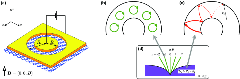
Figure 1: (a) The Corbino setup in graphene. Voltage source passes the current between the circular leads (yellow areas) via disk-shaped sample with the inner radii $R_{\rm i}$ and the outer radii $R_{\rm o}$. Uniform magnetic field ${\bf B}=(0,0,B)$ is perpendicular to the sample. Additional gate electrode (not shown) tunes the doping in the disk area. (b)–(d) Transport regimes for different fields and carrier concentrations $n_{E}$. At high fields, if doping is adjusted to a Landau level ($E=E_{n{\rm LL}}$, $n=0,\pm{}1,\dots$) resonance occurs (b). At low field but high doping (such that the cyclotron diameter $2r_{c}>R_{\rm o}-R_{\rm i}$), incoherent scattering along classical trajectory governs the transport (c).

The remaining parts of the paper are organized as follows. In Sec. II we present details of our numerical approach, which can be applied either in the idealized case where the electrostatic potential energy is a piecewise-constant function of the distance from the disk center, or in the more general case of smooth potentials. Our numerical results for both cases are presented in Sec. III. The conclusions are given in Sec. IV.

II Model and methods

II.1 Scattering of Dirac fermions

Our analysis starts with the wave equation for massless Dirac fermions in graphene at energy $E$ and uniform magnetic field $B$, which can be written as (for the $K$ valley)

$$\left[v_{F}\,(\mbox{\boldmath$p$}+e\mbox{\boldmath$A$})\cdot\mbox{\boldmath$\sigma$}+V(r)\right]\Psi=E\Psi,$$ (2)

where $v_{F}=\sqrt{3}\,t_{0}a/(2\hbar)\approx{}10^{6}\,$m$/$s is the energy-independent Fermi velocity in graphene (with $t_{0}=2.7\,$eV the nearest-neighbor hopping integral and $a=0.246\,$nm the lattice parameter), $\mbox{\boldmath$p$}=(p_{x},p_{y})$ is the in-plane momentum operator with $p_{j}=-i\hbar{}\partial_{j}$, we choose the symmetric gauge $\mbox{\boldmath$A$}=\frac{B}{2}(-y,x)$, and $\mbox{\boldmath$\sigma$}=(\sigma_{x},\sigma_{y})$, where $\sigma_{j}$ are the Pauli matrices. The electrostatic potential energy $V(r)$ depends only on distance from the origin in polar coordinates $(r,\varphi)$ and is given by

$$V(r)=-V_{0}\times\begin{cases}\,\frac{2^{m}|r-R_{\rm av}|^{m}}{|R_{\rm o}-R_{\rm i}|^{m}}&\text{if }\ |r\!-\!R_{\rm av}|\leqslant\frac{R_{\rm o}-R_{\rm i}}{2},\\ \,1&\text{if }\ |r\!-\!R_{\rm av}|>\frac{R_{\rm o}-R_{\rm i}}{2},\end{cases}$$ (3)

where we have defined $R_{\rm av}=(R_{\rm i}+R_{\rm o})/2$ with $R_{\rm i}$ and $R_{\rm o}$ being the inner and outer radii of the disk. We also note that the limit of $V_{0}\rightarrow\infty$ and $m\rightarrow\infty$ restores the familiar rectangular barrier of an infinite height Ryc09 ; Ryc10 .

Because of the symmetry, the wave function can be written in a form

$$\Psi_{j}(r,\varphi)=e^{i(j-1/2)\varphi}\left(\begin{array}[]{c}\chi_{a}\\ \chi_{b}e^{i\varphi}\\ \end{array}\right),$$ (4)

where $j=\pm{1/2},\pm{3/2},\dots$ is the total angular-momentum quantum number. In the leads, $r<R_{\rm i}$ or $r>R_{\rm o}$, the electrostatic potential energy is constant, $V(r)=-V_{0}$. In the case of electron doping, $E>-V_{0}$, the spinors $(\chi_{a},\chi_{b})^{T}$ for the incoming (i.e., propagating from $r=0$) and outgoing (i.e., propagating from $r=\infty$) waves are given, up to the normalization, by

$$\chi_{j}^{\rm in}\!=\left(\begin{array}[]{c}H_{j-1/2}^{(2)}(kr)\\ iH_{j+1/2}^{(2)}(kr)\\ \end{array}\right),\ \ \ \chi_{j}^{\rm out}\!=\left(\begin{array}[]{c}H_{j-1/2}^{(1)}(kr)\\ iH_{j+1/2}^{(1)}(kr)\\ \end{array}\right),$$ (5)

where $H_{\nu}^{(1)}(\rho)$ [$H_{\nu}^{(2)}(\rho)$] is the Hankel function of the first [second] kind, $k=|E+V_{0}|/(\hbar{}v_{F})$, and we have set $B=0$ in the leads hankfoo . (The wavefunctions for $B\neq{}0$ are given explicitly in Refs. Che06 ; Ryc10 .) Full wavefunctions in the leads, for a given $j$, can be written as

$$\chi_{j}^{({\rm i})} =\chi_{j}^{\rm in}+r_{j}\chi_{j}^{\rm out},\ r<R_{\rm i},$$ (6)

$$\chi_{j}^{({\rm o})} =t_{j}\chi_{j}^{\rm in},\ r>R_{\rm o},$$ (7)

with the reflection (and transmission) amplitudes $r_{j}$ (and $t_{j}$).

For the disk area, $R_{\rm i}<r<R_{\rm o}$, we have $B\neq{}0$ and the position-dependent $V(r)$. Eq. (2) brought us to the system of ordinary differential equations for spinor components

$$\chi_{a}^{\prime} =\left(\frac{j-1/2}{r}+\frac{eBr}{2\hbar}\right)\chi_{a}+i\,\frac{E-V(r)}{\hbar{}v_{F}}\chi_{b},$$ (8)

$$\chi_{b}^{\prime} =i\,\frac{E-V(r)}{\hbar{}v_{F}}\chi_{a}-\left(\frac{j+1/2}{r}+\frac{eBr}{2\hbar}\right)\chi_{b},$$ (9)

which has to be integrated numerically for all $j$-s. To reduce round-off errors that occur in finite-precision arithmetic due to exponentially growing (or decaying) spinor components, we have divided the interval $R_{\rm i}\dots R_{\rm o}$ into $M$ equally wide parts, bounded by $R_{\rm i}^{(l)}<r<R_{\rm o}^{(l)}$, with $l=0,1,\dots,M-1$, and

$$R_{\rm i}^{(l)}=R_{\rm i}+l\,\frac{R_{\rm o}-R_{\rm i}}{M},\ \ \ \ \ R_{\rm o}^{(l)}=R_{\rm i}^{(l+1)}.$$ (10)

The resulting wave function for the $l$-th interval then has the form

$$\chi_{j}^{(l)}=A_{j}^{(l)}\chi_{j}^{(l),{\rm I}}+B_{j}^{(l)}\chi_{j}^{(l),{\rm II}},$$ (11)

where $\chi_{j}^{(l),{\rm I}}$, $\chi_{j}^{(l),{\rm II}}$ denote the two linearly independent solutions that we obtained numerically by solving Eqs. (8,9) with two different initial conditions, $\left.\chi_{j}^{(l),{\rm I}}\right|_{r=R_{\rm i}^{(l)}}=(1,0)^{T}$ and $\left.\chi_{j}^{(l),{\rm II}}\right|_{r=R_{\rm i}^{(l)}}=(0,1)^{T}$. $A_{j}^{(l)}$ and $B_{j}^{(l)}$ are arbitrary complex coefficients.

The matching conditions, namely

$$\chi_{j}^{({\rm i})}(R_{\rm i}) =\chi_{j}^{(0)}(R_{\rm i}),$$ (12)

$$\chi_{j}^{(l)}(R_{\rm o}^{(l)}) =\chi_{j}^{(l+1)}(R_{\rm i}^{(l+1)}),\ \ \ \ l=0,\dots,M-2,$$ (13)

$$\chi_{j}^{(M-1)}(R_{\rm o}) =\chi_{j}^{({\rm o})}(R_{\rm o}),$$ (14)

are equivalent to the system of $2M+2$ linear equations for the unknowns $A_{j}^{(0)}$, $B_{j}^{(0)}$, …, $A_{j}^{(M-1)}$, $B_{j}^{(M-1)}$, $r_{j}$, and $t_{j}$, which can be written as

$$\left[\begin{matrix}-\chi_{j,a}^{\rm out}(R_{\rm i})&\chi_{j,a}^{(0),{\rm I}}(R_{\rm i}^{(0)})&\chi_{j,a}^{(0),{\rm II}}(R_{\rm i}^{(0)})&&&&\\ -\chi_{j,b}^{\rm out}(R_{\rm i})&\chi_{j,b}^{(0),{\rm I}}(R_{\rm i}^{(0)})&\chi_{j,b}^{(0),{\rm II}}(R_{\rm i}^{(0)})&&&&\\ 0&\chi_{a}^{(0),{\rm I}}(R_{\rm o}^{(0)})&\chi_{j,a}^{(0),{\rm II}}(R_{\rm o}^{(0)})&&&&\\ 0&\chi_{b}^{(0),{\rm I}}(R_{\rm o}^{(0)})&\chi_{j,b}^{(0),{\rm II}}(R_{\rm o}^{(0)})&\ddots&&&\\ &&&\ddots&\chi_{j,a}^{(\overline{M}),{\rm I}}(R_{\rm i}^{(\overline{M})})&\chi_{j,a}^{(\overline{M}),{\rm II}}(R_{\rm i}^{(\overline{M})})&0\\ &&&&\chi_{j,b}^{(\overline{M}),{\rm I}}(R_{\rm i}^{(\overline{M})})&\chi_{j,b}^{(\overline{M}),{\rm II}}(R_{\rm i}^{(\overline{M})})&0\\ &&&&\chi_{a}^{(\overline{M}),{\rm I}}(R_{\rm o}^{(\overline{M})})&\chi_{j,a}^{(\overline{M}),{\rm II}}(R_{\rm o}^{(\overline{M})})&-\chi_{j,a}^{\rm in}(R_{\rm o})\\ &&&&\chi_{b}^{(\overline{M}),{\rm I}}(R_{\rm o}^{(\overline{M})})&\chi_{j,b}^{(\overline{M}),{\rm II}}(R_{\rm o}^{(\overline{M})})&-\chi_{j,b}^{\rm in}(R_{\rm o})\\ \end{matrix}\right]$$

$$\times\ \left[\begin{matrix}r_{j}\\ A_{j}^{(0)}\\ B_{j}^{(0)}\\ \vdots\\ A_{j}^{(M-1)}\\ B_{j}^{(M-1)}\\ t_{j}\\ \end{matrix}\right]=\left[\begin{matrix}\,\chi_{j,a}^{\rm in}(R_{\rm i})\,\\ \,\chi_{j,b}^{\rm in}(R_{\rm i})\,\\ 0\\ \vdots\\ 0\\ \end{matrix}\right],$$ (15)

where we have explicitly written the spinor components of the relevant wavefunctions appearing in Eqs. (12), (13), and (14) and defined $\overline{M}=M-1$.

Analogously, assuming the scattering from $r=\infty$, we replace Eqs. (6,7) with

$$\chi_{j}^{({\rm i})} =t_{j}^{\prime}\chi_{j}^{\rm out},\ r<R_{\rm i},$$ (16)

$$\chi_{j}^{({\rm o})} =\chi_{j}^{\rm out}+r_{j}^{\prime}\chi_{j}^{\rm in},\ r>R_{\rm o},$$ (17)

and follow the consequtive steps mentioned above to obtain the linear system

$${\mathbb{A}}_{j}\times\left[\begin{matrix}t_{j}^{\prime}\\ {A_{j}^{(0)}}^{\prime}\\ {B_{j}^{(0)}}^{\prime}\\ \vdots\\ {A_{j}^{(M-1)}}^{\prime}\\ {B_{j}^{(M-1)}}^{\prime}\\ r_{j}^{\prime}\\ \end{matrix}\right]=\left[\begin{matrix}0\\ \vdots\\ 0\\ \,\chi_{j,a}^{\rm out}(R_{\rm o})\,\\ \,\chi_{j,b}^{\rm out}(R_{\rm o})\,\\ \end{matrix}\right],$$ (18)

where $\mathbb{A}_{j}$ is the main matrix as in Eq. (15) and $r_{j}^{\prime}$ ($t_{j}^{\prime}$) being the reflection (transmission) amplitude for the scattering from the outer lead. (Note that the elements of the $\mathbb{A}_{j}$ matrix are unchanged; hence, Eqs. (8,9) need only to be integrated numerically once for a given $j$.) The scattering matrix,

$${\mathbb{S}}_{j}=\left[\begin{matrix}r&t^{\prime}\\ t&r^{\prime}\\ \end{matrix}\right],$$ (19)

contains all the amplitudes mentioned above. Conservation of electric xharge implies the unitarity of the ${\mathbb{S}}_{j}$ matrix, ${\mathbb{S}}_{j}{\mathbb{S}}_{j}^{\dagger}={\mathbb{S}}_{j}^{\dagger}{\mathbb{S}}_{j}={\mathbb{I}}$ (where ${\mathbb{I}}$ is the identity matrix). The deviation from unitarity due to numerical errors, i.e., $\mbox{max}_{j}\left(|\epsilon_{j}|\right)$ with $\epsilon_{j}=\mbox{Tr}\left({\mathbb{S}}_{j}^{\dagger}{\mathbb{S}}_{j}-{\mathbb{I}}\right)$, provides a useful measure of the computational accuracy.

Since linear systems for different $j$-s are decoupled, numerous software packages can be used to find their solutions up to machine precision. We use the double precision LAPACK routine zgesv, see Ref. zgesv99 . The transmission probabilities are calculated as $T_{j}=|t_{j}|^{2}$.

For heavily-doped leads ($V_{0}\rightarrow\infty$) the wave functions given by Eq. (5) simplify to

$$\chi_{j}^{({\rm in})}=\frac{e^{iKr}}{\sqrt{r}}\left(\begin{array}[]{c}1\\ 1\\ \end{array}\right),\ \ \ \ \chi_{j}^{({\rm out})}=\frac{e^{-iKr}}{\sqrt{r}}\left(\begin{array}[]{c}1\\ -1\\ \end{array}\right),$$ (20)

with $K=|E+{}V_{0}|/(\hbar{}v_{F})\rightarrow{}\infty$. In particular, for $m\rightarrow\infty$ and $M=1$, closed-form expressions for $T_{j}$-s were found, either for $B=0$ Ryc09 or for $B\neq{}0$ Ryc10 . However, we have found that the available implementations of hypergeometric functions that occur in these expressions lead to numerical stability problems when calculating thermoelectric properties in the quantum Hall regime. Therefore, a procedure described in this subsection is applied directly in all the following numerical examples, with wave functions in the leads given by Eqs. (6,7) for $m<+\infty$ (smooth potential barriers). For $m\rightarrow\infty$ (rectangular barrier), both the finite and infinite doping in the leads are studied for comparison.

The numerical integration of Eqs. (8,9) was performed for each of $M=20$ intervals using a standard fourth-order Runge-Kutta (RK4) algorithm. For $R_{\rm o}=2R_{\rm i}=1000\,$nm and $B<0.5\,$T, a spatial step of $0.5\,$pm was sufficient to reduce the unitarity error down to $\mbox{max}\left(|\epsilon_{j}|\right)<10^{-8}$. The summation over the modes was stopped when $T_{j}<10^{-7}$. The Dormand-Prince method simfoo was also implemented; however, no significant differences in the transmission probabilities were found compared to RK4.

II.2 Thermoelectric characteristics

Within the Landauer-Büttiker formalism, the linear-response conductance Lan57 ; But85 and other thermoelectric properties Pau03 ; Esf06 can be calculated from the transmission-energy dependence

$${\cal T}(E)=\sum_{j=-j_{\rm max}}^{j_{\rm max}}{}T_{j}(E),$$ (21)

where $j_{\rm max}=\lfloor{}KR_{\rm i}\rfloor-\frac{1}{2}$ (for heavily-doped leads, $j_{\rm max}\rightarrow{}\infty$), via dimensionless integrals

$${L}_{n}=(k_{B}T)^{-n}\int{}dE\,{\cal T}(E)\left(-\frac{\partial{}f_{\rm FD}}{\partial{}E}\right)(E-\mu)^{n},$$ (22)

with $f_{\rm FD}(\mu,T,E)=1/\left[\,\exp\left((E\!-\!\mu)/k_{B}T\right)+1\,\right]$ the Fermi-Dirac distribution function and the chemical potential $\mu$. In particular,

$$G =\frac{g_{s}g_{v}e^{2}}{h}L_{0}\ \ \ \ (\text{the conductance}),$$ (23)

$$S =\left.\frac{dU}{dT}\right|_{I=0}=\frac{k_{B}L_{1}}{eL_{0}}\ \ \ \ (\text{the Seebeck coefficient}),$$ (24)

$${\cal L} =\frac{K_{\rm el}}{TG}=\frac{k_{B}^{2}(L_{0}L_{2}\!-\!L_{1}^{2})}{e^{2}L_{0}^{2}}\ \ \ (\text{the Lorentz number}),$$ (25)

where $g_{s}=g_{v}=2$ are spin and valley degeneracies, $dU/dT|_{I=0}$ is the voltage derivative with respect to the temperature difference between the leads at zero electric current, and $K_{\rm el}$ is the electronic part of the thermal conductance.

For zero temperature, Eq. (23) reduces to

$$G(T\!\rightarrow{}\!0)=g_{0}{\cal T}(E_{F}),$$ (26)

where we have defined the conductance quantum $g_{0}=4e^{2}/h$ and the Fermi energy $E_{F}$ ($=\mu$ for $T=0$). In turn, the zero-temperature conductance provides a direct insight into the transmission-energy dependence.

For some specific ${\cal T}(E)$, integrals in Eqs. (24,25) can be calculated analytically. In particular, ${\cal T}(E)\approx{}$const leads to $S\approx{}0$ and ${\cal L}\approx{}{\cal L}_{0}=(\pi^{2}/3)\,k_{B}^{2}/e^{2}$, which defines the Wiedemann-Franz law for metals Kit05 . For gapless Dirac systems, the corresponding approximation is ${\cal T}(E)\approx{}{\cal C}|E|$, with a constant ${\cal C}>0$, for which both $S$ and ${\cal L}$ can be expressed by the polylogarithm function of $\mu/k_{B}T$ Sus18 , with a universal (${\cal C}$-independent) maxima $S_{\rm max}\simeq{}1.0023\,k_{B}/e$ and ${\cal L}_{\rm max}\simeq{}2.3721\,{\cal L}_{0}$. The latter value was first reported in the context of $d$-wave systems Sha03 , before being found again for Dirac materials Sai07 ; Yos15 ; Ing15 .

In the presence of a transport gap, one can consider a simplified model for ${\cal T}(E)$, given by

$${\cal T}_{\rm model}(E)={\cal A}\delta(E)+{\cal B}\delta(E-\Delta{}E),$$ (27)

where ${\cal A}>0$, ${\cal B}>0$ are the constants, and $\delta(x)$ is the Dirac delta function. Generalizing the derivations presented in Refs. Sus19 and Ryc21a to the asymmetric case (${\cal A}\neq{\cal B}$), one finds easily

$$\frac{S_{\rm max}\!-\!S_{\rm min}}{2} \simeq{}\frac{k_{B}}{e}\!\left[\sqrt{u(u\!-\!1)}-\ln(\sqrt{u}+\sqrt{u\!-\!1})\right],$$ (28)

$${\cal L}_{\rm max} \simeq{}\left(\frac{k_{B}}{e}\right)^{2}u^{2}=\left(\frac{\Delta{}E}{2eT}\right)^{2},$$ (29)

where $u=\Delta{}E/(2k_{B}T)$ and the asymptotic equalities correspond to $u\gg{}1$. The remaining symbols in Eq. (28) are the maximum ($S_{\rm max}$) and the minimum ($S_{\rm min}$) Seebeck coefficient in the interval of $0<\mu<\Delta{E}$. Note that the right-hand sides in Eqs. (28) and (29) depend only on $u$ and the fundamental constants.

In a case where more $\delta$-shaped peaks appear in the transmission spectrum ${\cal T}(E)$, as might be expected for the quantum Hall regime, the approximations given by Eqs. (28) and (29) are also valid, provided that a gap is identified with the maximum interval between the peaks ($\Delta{}E=\Delta{}E_{\rm max}$). The monotonicity of the right-hand sides in Eqs. (28) and (29) guarantees that the resulting approximations, for $\Delta{}E=\Delta{}E_{\rm max}$, correspond to the global maxima of the relevant quantities (i.e., the thermopower amplitude and the Lorentz number) as functions of $\mu$.

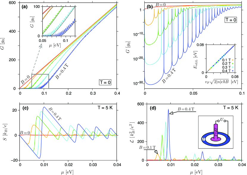
Figure 2: (a,b) Zero-temperature conductance, (c) the Seebeck coefficient and (d) the Lorentz number, both for $T=5\,$K, for the system of Fig. 1 with $R_{\rm o}=2R_{\rm i}=1000\,$nm and the rectangular potential barrier [$V_{0},m\rightarrow{}\infty$; see Eq. (3)] displayed as functions of the chemical potential. The magnetic field is varied from $B=0$ (red solid lines in all plots) to $B=0.4\,$T (blue solid lines) with the steps of $0.1\,$T. Inset in (a) is a zoom-in, with black dashed lines depicting the incoherent conductance (see Appendix A). (b) shows same data as (a), but using the semilogarithmic scale, with the inset presenting positions of the actual transmission maxima for $B>0$ ($E_{n{\rm LL}}$) versus the values for bulk graphene [see Eq. (30)]. A setup for thermoelectric measurements is also depicted [see inset in (d)].

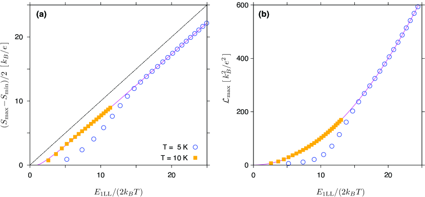
Figure 3: (a) Maximum amplitude of the Seebeck coefficient and (b) maximum Lorentz number for same system as in Fig. 2 at $T=5\,K$ (open symbols) and $T=10\,$K (closed symbols) as functions of the maximum interval between Landau levels of $\Delta{}E_{\rm max}\equiv{}E_{1{\rm LL}}=|E_{0{\rm LL}}-E_{\pm{}1{\rm LL}}|$. Solid lines depict the asymptotic expressions given in Eqs. (28) and (29). Dashed line in (a) corresponds to the Goldsmid-Sharp relation, see Eq. (1), with $E_{g}=E_{1{\rm LL}}$.

III Results and discussion

III.1 Zero-temperature conductance

Before discussing the thermoelectric properties, we present zero-temperature conductance spectra, wjich are related to the transmission-energy dependence via Eq. (26), and thus represent the input data for the calculatoin of the Seebeck coefficient and the Lorentz number. For the rectangular barrier of infinite height, $m,V_{0}\rightarrow{}\infty$ in Eq. (3), the spectra are particle-hole symmetric, and it is sufficient to consider $\mu\geqslant{}0$.

In Figs. 2(a) and 2(b) we display the disk conductance as a function of $\mu=E_{F}$ for $T=0$. Resonances via Landau levels, centered near energies very close to the corresponding values for bulk graphene,

$$E_{n{\rm LL}}\approx{}E_{n{\rm LL}}^{{\rm bulk}}=\mbox{sgn}(n)v_{F}\sqrt{2|n|e\hbar{}B},$$ (30)

where $n$ is an integer (without loss of generality, we hereinafter suppose $B>0$), are clearly visible starting from a moderate value of $B=0.1\,$T. More generally, one can expect the resonances to be visible up to the $n$-th one if

$$E_{n{\rm LL}}\lesssim{}E_{c,1}=\frac{v_{F}eB}{2}\left(R_{\rm o}-R_{\rm i}\right),$$ (31)

where $E_{c,1}$ denotes the threshold energy, below which the cyclotron diameter $2r_{c}=2|E_{F}|/(v_{F}eB)<R_{\rm o}-R_{\rm i}$ and the incoherent transmission vanishes (see Appendix A). For instance, for $R_{\rm o}=2R_{\rm i}=1000\,$nm discussed throughout the paper, Eq. (31) gives

$$|n|\lesssim{}47.47\times{}B\,[\text{T}],$$ (32)

coinciding with the number of well-separated maxima visualized in semi-logarithmic scale in Fig. 2(b).

It is also visible, for $|E_{F}|>E_{c,1}$, that the actual $G$ grows rapidly with increasing $|E_{F}|$, closely following the prediction for incoherent transport [see Fig. 2(a) and the inset]. This observation leads to the question whether $E_{1LL}$, or rather $2E_{c,1}$, defines the relevant transport gap to be substituted into Eqs. (28) and (29)?

This problem is solved via the numerical analysis of $S$ and ${\cal L}$ which will be presented next.

III.2 Thermopower and the Lorentz number

The Seebeck coefficient and the Lorentz number, calculated from Eqs. (24) and (25) for $T=5\,$K, are shown in Figs. 2(c) and 2(d) as functions of the chemical potential. Again, the particle-hole symmetry of ${\cal T}(E)$ guarantees that $S(\mu)$ is odd and ${\cal L}(\mu)$ is even on $\mu\rightarrow{}-\mu$, and it is sufficient to consider $\mu\geqslant{}0$.

In the quantum Hall regime, i.e., for $|\mu|<E_{c,1}$, see Eq. (31), the ${\cal T}(E)$ function consists of narrow peaks, each centered at $E_{n{\rm LL}}$ (see previous subsection). In such a case, reliable numerical estimations of the integrals $L_{0}$, $L_{1}$, and $L_{2}$ [see Eq. (22)] requires sufficiently dense sampling of ${\cal T}(E)$ near $E\approx{}E_{n{\rm LL}}$.

The analytic structure of Eqs. (24) and (25) results in the following features visible in Figs. 2(c) and 2(d): First, each of the consecutive intervals, i.e., $E_{0{\rm LL}}<E<E_{1{\rm LL}}$, $E_{1{\rm LL}}<E<E_{2{\rm LL}}$, etc., contains a local minimum and a local maximum of $S$, surrounding an odd zero of $S$ (even zeros occur for the resonances at $\mu\approx{}E_{n{\rm LL}}$), which corresponds to a local maximum of ${\cal L}$. Second, the global extrema (corresponding to $S_{\rm min}$, $S_{\rm max}$, or ${\cal L}_{\rm max}$) are all in the first interval, $E_{0{\rm LL}}<E<E_{1{\rm LL}}$, characterized by the maximum width ($\Delta{}E_{\rm max}\equiv{}E_{1{\rm LL}}-E_{0{\rm LL}}=E_{1{\rm LL}}$).

In Fig. 3 we plot the values of $(S_{\rm max}-S_{\rm min})/2$ and ${\cal L}_{\rm max}$ against the dimensionless variable $E_{1{\rm LL}}/(2k_{B}{}T)$, for the two values of $T=5\,$K and $10\,$K. Results of the numerical integration and subsequent optimization with respect to the chemical potential $\mu$ [datapoints] closely follow the approximations given in Eqs. (28,29) [solid lines], starting from $E_{1{\rm LL}}/(2k_{B}{}T)\gtrsim{}10$. The Goldsmid-Sharp formula [dashed line] produces a noticeable offset when compared to the Landauer-Büttiker results, but can still be used as a less accurate approximation for $(S_{\rm max}-S_{\rm min})/2$ for large $E_{1{\rm LL}}/(2k_{B}{}T)$.

These results support our conjecture that the model ${\cal T}(E)$, given by Eq. (27), is able to reproduce the basic thermoelectric properties of graphene disk in the quantum Hall regime. Although it may seem surprising, at least at first glance, that the model ${\cal T}(E)$ with $\Delta{}E=E_{1{\rm LL}}$ reproduces the actual numerical results, whereas the energy scale of $2E_{c,1}\gg{}E_{1{\rm LL}}$ [see Eq. (31)] seems to be irrelevant. However, for thermal excitation energies $k_{B}{}T\ll{}E_{1{\rm LL}}\ll{}2E_{c,1}$, the detailed behavior of the actual ${\cal T}(E)$ [see Eq. (21)] for $E-E_{0{\rm LL}}=E\lesssim{}-k_{B}T$ or $E-E_{1{\rm LL}}\gtrsim{}k_{B}{}T$ does not affect the integrals $L_{0}$, $L_{1}$, $L_{2}$ (note that the full width at half maximum for $-\partial{}f_{\rm FD}/\partial{}E$ in Eq. (22) is $\approx{}\!3.53\,k_{B}{}T\,$) when $0<\mu<E_{1{\rm LL}}$). For this reason, a model with $\Delta{}E=E_{1{\rm LL}}$ captures the essential features of the actual ${\cal T}(E)$, while focussing on the thermoelectric properties considered here.

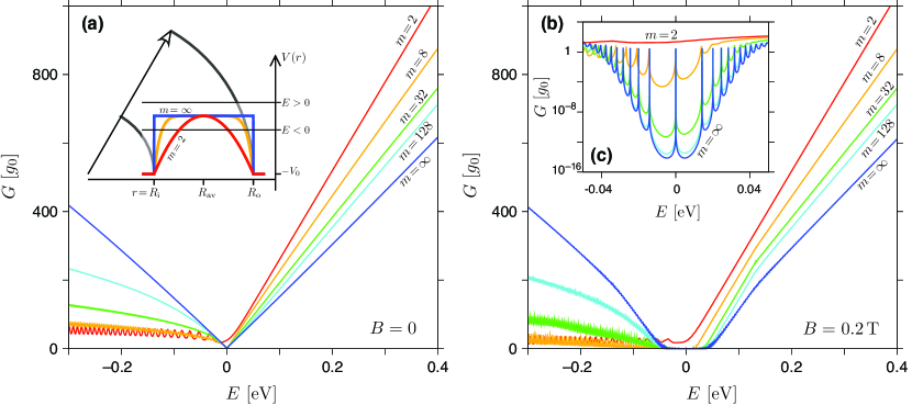
Figure 4: Zero-temperature conductance at (a) $B=0$ and (b) $B=0.2\,$T versus the Fermi energy. The disk radii are same as Fig. 2, the barrier height [see Eq. (3)] is fixed at $V_{0}=t_{0}/2=1.35\,$eV, the parameter $m$ is specified for each line. Inset in (a) shows selected potential profiles. (c) Zoom-in, for low energies, with same datasets as in (b) displayed in semi-logarithmic scale.

III.3 Smooth potential barriers

For the sake of completeness, in this section we also revisit the effects of smooth potential barriers, considered earlier for zero magnetic field Ryc22 . The electrostatic potential energy is given by Eq. (3), where the barrier height is fixed at $V_{0}=t_{0}/2=1.35\,$eV (for selected profiles for $m=2$, $8$, and $\infty$, see Fig. 4) and the radii $R_{\rm o}=2R_{\rm i}=1000\,$nm again.

For a finite barrier height, the particle-hole symmetry of the conductance spectrum $G(E)$ is absent, even for the rectangular barrier ($m=\infty$). However, for sufficiently low energies $|E|\ll{}V_{0}$ and large $m$, the Fermi wavelength $\lambda_{F}=hv_{F}/|E|$ becomes longer than a characteristic length scale of a potential jump, i.e., $\Delta{}r=(L-L_{\rm eff})/2$ where the sample length is $L=R_{\rm o}-R_{\rm i}=500\,$nm, and

$${L_{\rm eff}^{(m)}}=L\left(\frac{\hbar{}v_{F}}{LV_{0}}\right)^{1/m}$$ (33)

is the so-called diffusive length defined via $V(R_{\rm av}\pm{}L_{\rm eff}/2)=-\hbar{}v_{F}/L$ (see Ref. Ryc21b ). The value of $\hbar{}v_{F}/L$ can be attributed to the energy uncertainty corresponding to a typical time of flight $\sim{}L/v_{F}$ (up to the order of magnitude). We further note that $L_{\rm eff}^{(m)}\rightarrow{}L$ for $m\rightarrow{}\infty$. If $\lambda_{F}\gg{}\Delta{}r$, the potential profile can be considered as approximately flat, and the approximate symmetry upon $E\rightarrow{}-E$ can be observed for the corresponding zero-field spectra shown in Fig. 4(a).

For $B=0.2\,$T, see Figs. 4(b) and 4(c), the approximate symmetry is also visible. In addition, it is worth noting that for $\lambda_{F}\gg{}\Delta{}r$ the lowest LLs are well pronounced, and their positions are almost unaffected compared to the infinite-barrier case [see previous subsection, Fig. 2(b)].

In both cases, i.e., for $B=0$ and $B=0.2\,$T, the presence of two circular p-n junctions for $E<0$ leads to a suppressed conductance compared to $E>0$, with well-pronounced conductance oscillations due to quasi-bounded states (especially for smaller $m$). Due to such an asymmetry, the global conductance minimum $G_{\rm min}$ in the quantum Hall regime is typically reached in the energy interval of $-E_{1{\rm LL}}<E<0$, with the exception of the parabolic profile ($m=2$), for which resonances with LLs are obliterated.

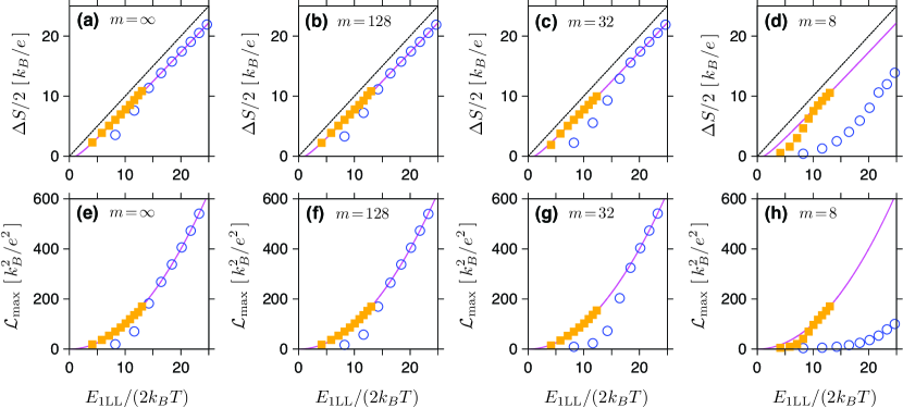
Figure 5: (a)–(d) Maximum amplitude of the Seebeck coefficient $\Delta{}S=(S_{\rm max}-S_{\rm min})/2$ and (e)–(h) maximum Lorentz number for same system as in Fig. 4 and selected values of the exponent $m$ defining the potential profile [see Eq. (3)] displayed as the bulk Landau-level energy $E_{1{\rm LL}}$ obtained from Eq. (30) with $n=1$. The line/color encoding is same as in Fig. 3.

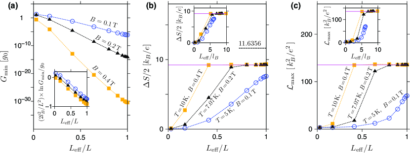
Figure 6: (a)–(c) Thermoelectric characteristics of the disk with smooth potential barriers in the quantum Hall regime displayed versus $L_{\rm eff}$ given by Eq. (33). (a) The minimum zero-temperature conductance reached for $-E_{1{\rm LL}}<E<0$, with inset visualizing the scaling according to $G_{\rm min}\propto{}\exp(-\frac{1}{2}L_{\rm eff}^{2}/l_{B}^{2})$ with $l_{B}=\sqrt{\hbar/eB}$ the magnetic length. (b) The maximum thermopower amplitude. (c) The maximum Lorentz number. Insets in (b,c) show same data as functions of the rescaled length $L_{\rm eff}/l_{B}$. The magnetic field is varied between the datasets (see datapoints, dashed lines are guide for the eye only). Additionally, in (b,c) the temperature is varied to keep the constant $E_{1{\rm LL}}/(2k_{B}{}T)\simeq{}11.6356$. Solid horizontal lines in (b,c) mark the values following from Eqs. (28) and (29).

The consequences of the above-mentioned features of $G(E)$ for thermoelectric properties are discussed next.

In Fig. 5 we show pairs of plots analogous to those shown in Fig. 3, i.e., the thermopower amplitude $\Delta{}S=(S_{\rm max}-S_{\rm min})/2$, and the maximum Lorentz number ${\cal L}_{\rm max}$, both displayed as functions of the dimensionless quantity $E_{1{\rm LL}}/(2k_{B}{}T)$. This time, a step height is finite and four values of the exponent $m$ (specified for each panel) are chosen. For sufficiently large $E_{1{\rm LL}}/(2k_{B}{}T)$, the approximations of Eqs. (28) and (29) [solid lines] are closely followed by the actual datapoints also for smooth potentials ($m<+\infty$); we further note that the agreement is generally better for $T=5\,$K [solid symbols] than for $T=10\,$K [open symbols].

The effect of $L_{\rm eff}/L<1$ corresponding to $m<+\infty$, see Eq. (33), and quantifying the potential smoothness, is further illustrated in Fig. 6, where we show selected thermoelectric properties, $G_{\rm min}$, $\Delta{}S$, and ${\cal L}_{\rm max}$, as functions of $L_{\rm eff}/L$. Each dataset corresponds to a fixed magnetic field ($B=0.1\,$T, $0.2\,$T, or $0.4\,$T), while the exponent $m$ is varied from $m=2$ to $512$, with an additional datapoint for rectangular barrier ($m=\infty$) placed at $L_{\rm eff}/L=1$. For finite-temperature characteristics, $\Delta{}S$ and ${\cal L}_{\rm max}$, we set $T=5\,K$ for $B=0.1\,$T; otherwise, $T$ is chosen to keep the constant $E_{1{\rm LL}}/(2k_{B}T)$ ratio (a quantity determining the approximate values $\Delta{}S$ and ${\cal L}_{\rm max}$ via Eqs. (28,29)).

Remarkably, the datasets for different $B$ reveal some common behavior upon a proper rescaling; see three insets in Figs. 6(a), 6(b), and 6(c). In the first plot, it is easy to see that the conductance away from the resonances with LLs behaves approximately as $G_{\rm min}\propto{}\exp(-\frac{1}{2}L_{\rm eff}^{2}/l_{B}^{2})$. In the next two plots, the datasets for the finite-temperature characteristics ($\Delta{}S$ and ${\cal L}_{\rm max}$) come much closer to each other if plotted as functions of $L_{\rm eff}/l_{B}$ (where $l_{B}=\sqrt{\hbar/eB}\simeq{}25.656\,$nm$\,\times{}(B\,[$T$])^{-1/2}$ is the magnetic length) than if simply plotted as functions of $L_{\rm eff}$.

In addition, the behavior of $G_{\rm min}$ further validates the numerical stability of the approach presented in Sec. II. Namely, the value of $G_{\rm min}/g_{0}\sim{}10^{-30}$ corresponds to the transmission amplitude $|t_{j}|\sim{}10^{-15}$, which coincides with a typical round-off error in double precision arithmetic. This is also a reason why we have limited our discussion to $B\leqslant{}0.4\,$T (or, equivalently, $L/l_{B}\leqslant{}12.33$ for $L=500\,$nm). For higher $B$, one must use numerical tools employing multiple precision mpack . In such a case, a significant slowdown of the computations can be expected.

From a physical point of view, the considered values of $B$ lead to the Zeeman splitting of $\Delta{}E_{Z}=g\mu_{B}{}B\approx{}1.16\cdot{}10^{-4}\,$eV$\times{}B\,[$T$]\ll{}E_{1{\rm LL}}$, with $g\simeq{}2$ and $\mu_{B}=e\hbar/(2m_{e})$ the Bohr magneton. Throughout this paper the Zeeman term is therefore neglected.

IV Conclusions

We have investigated selected thermoelectric properties of graphene-based Corbino disks in the presence of an external magnetic field. An efficient numerical scheme that allows the determination of these properties through mode matching for the Dirac equation, up to the magnetic fields that drive the system into the quantum Hall regime, using only a standard double precision arithmetic, is put forward.

Our results show that both the thermopower amplitude and the maximal Lorentz number are determined by the energy interval separating the $n=0$ and $n=\pm{}1$ Landau levels (LLs) divided by the absolute temperature, and the fundamental constants. (The ratio of the disk radii, as well as the detailed shape of the electrostatic potential profile, are irrelevant.) Approximate expressions for the two above-mentioned thermoelectric characteristics can be derived by assuming the transmission-energy dependence to be in the form of two Dirac-delta peaks, centered at the energies of $n=0$ and $n=1$ (or $n=-1$) LLs. In particular, the expression describing the thermopower amplitude can be regarded as a modified version of the well-known Goldsmid-Sharp relation for semiconductors. It appears that a disk-shaped graphene sample, coupled to the two reservoirs in local thermal equilibrium, can act as a thermometer measuring the small temperature difference between the reservoirs (provided that applied field and average temperature are known).

Our analysis is carried out within the Landauer-Büttiker formalism for noninteracting quasiparticles. This implies that the fractional quantum Hall effect (FQHE) is outside the scope of this work. Although transmission resonances with FQHE states have been observed in ultraclean graphene samples Zen19 , existing thermoelectric measurements for GaAs/AlGaAs disks Kob13 ; Rea20 indicate the presence of integer QHE states only. For this reason, a theoretical study of the thermoelectric signatures of integer QHE states had to be completed as a first step. Undoubtedly, generalizing the approach to include FQHE states would be a promising direction for future studies.

Author contributions

A.R. designed the algorithm, A.R. and P.W. developed the code and performed preliminary computations, K.R. organized the computations on the PL-Grid supercomputing infrastructure; all authors were involved in data analysis and manuscript preparation.

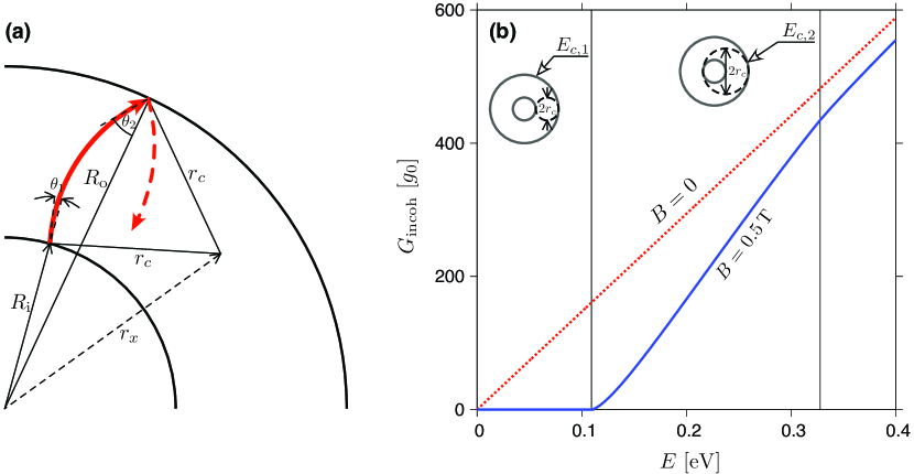
Figure 7: (a) Propagation between subsequent scatterings on interfaces at $r=R_{\rm i}$ and $r=R_{\rm o}$ (with incident angles $\theta_{1}$, $\theta_{2}$) in uniform magnetic field, defining the cyclotron orbit centered at $r=r_{x}$ with its radii $r_{c}$. (b) Incoherent conductance calculated from Eq. (34) for $B=0$ [dashed line] and $B=0.5\,$T [solid line]. The disk radii are $R_{\rm o}=2R_{\rm i}=1000\,$nm; a rectangular potential barrier is considered. Characteristic Fermi energies $E_{c,1}$ and $E_{c,2}$ mark with vertical lines correspond to $r_{c}=(R_{\rm o}-R_{\rm i})/2$ and $r_{c}=(R_{\rm i}+R_{\rm o})/2$ (respectively).

Appendix A Incoherent transport at magnetic field

Incoherent conductance ($G_{\rm incoh}$) is calculated below by adapting the method presented in Ref. Ryc22 for the uniform magnetic field case.

Due to the disk symmetry, the incident angles, $\theta_{1}$ for the interface at $r=R_{\rm i}$ and $\theta_{2}$ for the interface at $r=R_{\rm o}$ (see Fig. 7) remain constant (up to a sign) during multiple scattering between the two interfaces. In turn, for a multimode regime, summing in Eq. (26) can be approximated by averaging over the modes, leading to

$$G_{\rm incoh}=2g_{0}k_{F}R_{\rm i}\left\langle{}T_{12}\right\rangle,$$ (34)

where

$$\left\langle{}T_{12}\right\rangle=\frac{1}{2}\int_{u_{c}}^{1}du_{1}\frac{T_{1}T_{2}}{T_{1}+T_{2}-T_{1}T_{2}},$$ (35)

with

$$T_{j}=\frac{2\sqrt{1-u_{j}^{2}}}{1+\sqrt{1-u_{j}^{2}}},\ \ \ \ j=1,2,$$ (36)

being the transmission probabilities for a potential step of infinite height. The parameter $u_{1}=\sin\theta_{1}$ is further regarded as an independent variable. $u_{c}$ in Eq. (35) denotes the minimal value of $u_{1}$ above which the corresponding $u_{2}=\sin\theta_{2}$ satisfies $|u_{2}|\leqslant{}1$.

Assuming a constant electrostatic potential energy in the disk area, the trajectory between subsequent scatterings forms an arc, with the radii $r_{c}=|E|/(v_{F}eB)$ (the cyclotron radius for massless Dirac particle at a field $B>0$), centered at the distance $r_{x}$ from the origin. Solving the two triangles with a common edge $r_{x}$ (dashed line) and the opposite vertices in two scattering points, one easily finds

$$r_{x}^{2}=R_{\rm i}^{2}+r_{c}^{2}+2R_{\rm i}{}r_{c}\sin\theta_{1}$$ (37)

(for the triangle containing a scattering point at $r=R_{\rm i}$), and

$$r_{x}^{2}=R_{\rm o}^{2}+r_{c}^{2}-2R_{\rm o}{}r_{c}\sin\theta_{2}$$ (38)

(for the triangle containing a scattering point at $r=R_{\rm o}$), leading to

$$u_{2}=\sin\theta_{2}=\frac{R_{\rm o}^{2}-R_{\rm i}^{2}-2R_{\rm i}r_{c}u_{1}}{2R_{\rm o}r_{c}}.$$ (39)

Therefore, the value of $u_{c}$ in Eq. (35) is given by

$$u_{c}=\begin{cases}-1,&\text{if }\ r_{c}\geqslant{}\frac{R_{\rm i}+R_{\rm o}}{2}\\ \frac{R_{\rm o}^{2}-R_{\rm i}^{2}}{2R_{\rm i}r_{c}}-\frac{R_{\rm o}}{R_{\rm i}},&\text{if }\ \frac{R_{\rm i}+R_{\rm o}}{2}>r_{c}\geqslant{}\frac{R_{\rm o}-R_{\rm i}}{2}\\ 1,&\text{if }\ r_{c}<\frac{R_{\rm o}-R_{\rm i}}{2}\\ \end{cases}.$$ (40)

In a zero-field limit, we have $r_{c}\rightarrow{}\infty$, leading to $u_{c}=-1$ and $u_{2}\rightarrow{}-(R_{\rm i}/R_{\rm o})u_{1}$. In such a limit, the integral in Eq. (35) can be calculated analytically, leading to

$$G_{\rm incoh}(B\rightarrow{}0)=2g_{0}k_{F}R_{\rm i}\frac{(2a+\frac{1}{a})\arcsin{}a+3\sqrt{1-a^{2}}-\frac{\pi}{2}(a^{2}+2)}{1-a^{2}},\ \ \ \ \text{with }\ a=R_{\rm i}/R_{\rm o}.$$ (41)

The above reproduces a zero-field result reported in Ref. Ryc22 . For $B>0$, the integration needs to be performed numerically.

From geometric point of view, the limiting values of $r_{c}$ in Eq. (40), i.e., $r_{c,1}=(R_{\rm o}-R_{\rm i})/2$ and $r_{c,2}=(R_{\rm i}+R_{\rm o})/2$, indicate three distinct situation: (i) none of the circular trajectories originating from $r=R_{\rm i}$ can reach $r=R_{\rm o}$ (the $r_{c}<r_{c,1}$ case), (ii) trajectories with some incident angles $\theta_{1}$ may reach the second interface, but some cannot (the $r_{c,2}>r_{c}\geqslant{}r_{c,1}$ case), and (iii) all the trajectories originating from $r=R_{\rm i}$ reach $r=R_{\rm o}$ (the $r_{c}\geqslant{}r_{c,1}$ case).

Also in Fig. 7, we display $G_{\rm incoh}$ calculated numerically from Eq. (34) for $B=0$ and $B=0.5\,$T, with the remaining system parameters same as considered throughout the paper. The Fermi energies $E_{c,\alpha}=v_{F}eBr_{c,\alpha}$, $\alpha=1,2$, for the $B=0.5\,$T case, are mark with vertical lines. It can be shown that for $E\approx{}E_{c,1}$, the incoherent conductance behaves as

$$G_{\rm incoh}(E)\propto{}\Theta(E-E_{c,1})\left|E-E_{c,1}\right|^{3/2},$$ (42)

with $\Theta(x)$ being the Heaviside step function.

Remarkably (see the main text), $G_{\rm incoh}$ follows quite close the actual $G$ calculated via the numerical mode matching, but thermoelectric characteristics are ruled by the Landau levels, with their energies being unrelated to the value of $E_{c,1}$.

References

- (1) K. S. Novoselov, A. K. Geim, S. V. Morozov, D. Jiang, Y. Zhang, S. V. Dubonos, I. V. Grigorieva, and A. A. Firsov, Science 306, 666 (2004).
- (2) K. S. Novoselov, A. K. Geim, S. V. Morozov, D. Jiang, M. I. Katsnelson, I. V. Grigorieva, S. V. Dubonos, and A. A. Firsov, Nature 438, 197 (2005).
- (3) Y. Zhang, Y.-W. Tan, H. L. Stormer, and P. Kim, Nature 438, 201 (2005).
- (4) S. Das Sarma, S. Adam, E. H. Hwang, E. Rossi, Rev. Mod. Phys. 83, 407 (2011).
- (5) A. V. Rozhkov, G. Giavaras, Y. P. Bliokh, V. Freilikher, and F. Nori, Phys. Rep. 503, 77 (2011).
- (6) See, e.g.: M. I. Katsnelson, The Physics of Graphene. Second Edition, (Cambridge University Press, Cambridge, UK, 2020). DOI: https://doi.org/10.1017/9781108617567, Chapter 3.
- (7) G. H. Lee, D. K. Efetov, W. Jung, L. Ranzani, E. D. Walsh, T. A. Ohki, T. Taniguchi, K. Watanabe, P. Kim, D. Englund et al., Nature 586, 42 (2020).
- (8) T. Li, H. Da, X. Du, J. J. He, and X. Yan, J. Phys. D: Appl. Phys. 53, 115108 (2020).
- (9) Y. Ronen, T. Werkmeister, D. H. Najafabadi, A. T. Pierce, L. E. Anderson, Y. J. Shin, S. Y. Lee, Y. H. Lee, B. Johnson, K. Watanabe et al., Nat. Nanotechnol. 16, 563 (2021).
- (10) A. Schmitt, P. Vallet, D. Mele, M. Rosticher, T. Taniguchi, K. Watanabe, E. Bocquillon, G. Fève, J. M. Berroir, C. Voisin et al., Nat. Phys. XX, XXXX (2023).
- (11) C.-C. Kalmbach, J. Schurr, F. J. Ahlers, A. Müller, S. Novikov, N. Lebedeva, and A. Satrapinski, Appl. Phys. Lett. 105, 073511 (2014).
- (12) F. Lafont, R. Ribeiro-Palau, D. Kazazis, A. Michon, O. Couturaud, C. Consejo, T. Chassagne, M. Zielinski, M. Portail, B. Jouault et al., Nat. Commun. 6, 6806 (2015).
- (13) M. Kruskopf and R. E. Elmquist, Metrologia 55, R27 (2018).
- (14) M. Polini, F. Guinea, M. Lewenstein, H. C. Manoharan, and V. Pellegrini, Nat. Nanotechnol. 8, 625 (2013).
- (15) M. Mattheakis, C. A. Valagiannopoulos, and E. Kaxiras Phys. Rev. B 94, 201404(R) (2016).
- (16) D. J. Trainer, S. Srinivasan, B. L. Fisher, Y. Zhang, C. R. Pfeiffer, S.-W. Hla, P. Darancet, N. P. Guisinger, e-print: arXiv:2104.11334 (unpublished).
- (17) V. V. Cheianov and V. I. Fal’ko, Phys. Rev. B 74, 041403(R) (2006).
- (18) A. Rycerz, P. Recher, and M. Wimmer, Phys. Rev. B 80, 125417 (2009).
- (19) A. Rycerz, Phys. Rev. B 81, 121404(R) (2010).
- (20) E. C. Peters, A. J. M. Giesbers, M. Burghard, and K. Kern, Appl. Phys. Lett. 104, 203109 (2014).
- (21) B. Abdollahipour and E. Moomivand, Physica E 86 204 (2017).
- (22) Y. Zeng, J. I. A. Li, S. A. Dietrich, O. M. Ghosh, K. Watanabe, T. Taniguchi, J. Hone, and C. R. Dean, Phys. Rev. Lett. 122, 137701 (2019).
- (23) D. Suszalski, G. Rut, and A. Rycerz, J. Phys. Mater. 3, 015006 (2020).
- (24) M. Kamada, V. Gall, J. Sarkar, M. Kumar, A. Laitinen, I. Gornyi, and P. Hakonen, Phys. Rev. B 104, 115432 (2021).
- (25) Y. Yerin, V. P. Gusynin, S. G. Sharapov, and A. A. Varlamov, Phys. Rev. B 104, 075415 (2021).
- (26) P. Dollfus, V. H. Nguyen, and J. Saint-Martin, J. Phys.: Condens. Matter 27, 133204 (2015).
- (27) C. R. Wang, W.-S. Lu, L. Hao, W.-L. Lee, T.-K. Lee, F. Lin, I-C. Cheng, and J.-Z. Chen, Phys. Rev. Lett. 107, 186602 (2011).
- (28) Y. Y. Chien, H. Yuan, C. R. Wang, and W. L. Lee, Sci. Rep. 6, 20402 (2016).
- (29) P. S. Mahapatra, K. Sarkar, H. R. Krishnamurthy, S. Mukerjee, and A. Ghosh, Nano Lett. 17, 6822 (2017).
- (30) D. Suszalski, G. Rut, and A. Rycerz, Phys. Rev. B 97, 125403 (2018).
- (31) D. Suszalski, G. Rut, and A. Rycerz, J. Phys.: Condens. Matter 31, 415501 (2019).
- (32) P. Zong, J. Liang, P. Zhang, C. Wan, Y. Wang, and K. Koumoto, ACS Appl. Energy Mater. 3, 2224 (2020).
- (33) Y. B. Dai, K. Luo, and X. F. Wang, Sci. Rep. 10, 9105 (2020).
- (34) A. Jayaraman, K. Hsieh, B. Ghawri, P. S. Mahapatra, K. Watanabe, T. Taniguchi, and A. Ghosh, Nano Lett. 21, 1221 (2021).
- (35) A. S. Ciepielewski, J. Tworzydło, T. Hyart, and A. Lau, Phys. Rev. Research 4, 043145 (2022).
- (36) M.-J. Lee, J.-H. Ahn, J. H. Sung, H. Heo, S. G. Jeon, W. Lee, J. Y. Song, K.-H. Hong, B. Choi, S.-H. Lee, amd M.-H. Jo, Nature Commun. 7, 12011 (2016).
- (37) H. Sevinçli, Nano Lett. 17, 2589 (2017).
- (38) D. Qin, P. Yan, G. Ding, X. Ge, H. Song, and G. Gao, Sci. Rep. 8, 2764 (2018).
- (39) D. Li, Y. Gong, Y. Chen, J. Lin, Q. Khan, Y. Zhang, Y. Li, H. Zhang, and H. Xie, Nano-Micro Lett. 12, 36 (2020).
- (40) L. Hao and T. K. Lee, Phys. Rev. B 81, 165445 (2010).
- (41) H. J. Goldsmid and J. W. Sharp, J. Electron. Mater. 28, 869 (1999).
- (42) A. Rycerz, Materials 14, 2704 (2021).
- (43) S. Li, A. Levchenko, and A. V. Andreev, Phys. Rev. B 105, 125302 (2022).
- (44) Y. Barlas and K. Yang, Phys. Rev. B 85, 195107 (2012).
- (45) S. Kobayakawa, A. Endo, and Y. Iye, J. Phys. Soc. Jpn. 82, 053702 (2013).
- (46) N. d’Ambrumenil and R. H. Morf, Phys. Rev. Lett. 111, 136805 (2013).
- (47) M. Real, D. Gresta, C. Reichl, J. Weis, A. Tonina, P. Giudici, L. Arrachea, W. Wegscheider, and W. Dietsche, Phys. Rev. Applied 14, 034019 (2020).
- (48) A. Rycerz and P. Witkowski, Phys. Rev. B 104, 165413 (2021).
- (49) A. Rycerz and P. Witkowski, Phys. Rev. B 106, 155428 (2022).
- (50) Numerical evaluation of the Hankel functions, with , are performed employing the double-precision regular [irregular] Bessel function of the fractional order [] as implemented in Gnu Scientific Library (GSL), see: https://www.gnu.org/software/gsl/doc/html/specfunc.html#bessel-functions. For , we use or .
- (51) E. Anderson, Z. Bai, C. Bischof, S. Blackford, J. Demmel, J. Dongarra et al., LAPACK Users’ Guide, Third Edition (Society for Industrial and Applied Mathematics, Philadelphia, USA, 1999).
- (52) J. R. Dormand, J.R. and P. J. Prince, J. Comput. Appl. Math. 6, 19 (1980).
- (53) R. Landauer, IBM J. Res. Dev. 1, 223 (1957).
- (54) M. Büttiker, Y. Imry, R. Landauer, and S. Pinhas, Phys. Rev. B 31, 6207 (1985).
- (55) M. Paulsson and S. Datta, Phys. Rev. B 67, 241403(R) (2003).
- (56) K. Esfarjani and M. Zebarjadi, Phys. Rev. B 73, 085406 (2006).
- (57) C. Kittel, Introduction to Solid State Physics, 8th ed. (John Willey and Sons, New York, NY, USA, 2005); Chapter 6.
- (58) S. G. Sharapov, V. P. Gusynin, and H. Beck, Phys. Rev. B 67, 144509 (2003).
- (59) K. Saito, J. Nakamura, and A. Natori, Phys. Rev. B 76, 115409 (2007).
- (60) H. Yoshino and K. Murata, J. Phys. Soc. Jpn. 84, 024601 (2015).
- (61) M. Inglot A. Dyrdał, V. K. Dugaev, and J. Barnaś, Phys. Rev. B 91, 115410 (2015).
- (62) See, e.g.: M. Nakata, The MPACK (MBLAS/MLAPACK): A Multiple Precision Arithmetic Version of BLAS and LAPACK, version 0.7.0 (2012); URL: http://mplapack.sourceforge.net.