Mahakala: a Python-based Modular Ray-tracing and Radiative Transfer Algorithm for Curved Space-times

Abstract

We introduce Mahakala, a Python-based, modular, radiative ray-tracing code for curved space-times. We employ Google’s JAX framework for accelerated automatic differentiation, which can efficiently compute Christoffel symbols directly from the metric, allowing the user to easily and quickly simulate photon trajectories through non-Kerr metrics. JAX also enables Mahakala to run in parallel on both CPUs and GPUs and achieve speeds comparable to C-based codes. Mahakala natively uses the Cartesian Kerr-Schild coordinate system, which avoids numerical issues caused by the “pole” of spherical coordinates. We demonstrate Mahakala’s capabilities by simulating the 1.3 mm wavelength images (the wavelength of Event Horizon Telescope observations) of general relativistic magnetohydrodynamic simulations of low-accretion rate supermassive black holes. The modular nature of Mahakala allows us to easily quantify the relative contribution of different regions of the flow to image features. We show that most of the emission seen in 1.3 mm images originates close to the black hole. We also quantify the relative contribution of the disk, forward jet, and counter jet to 1.3 mm images.

1 Introduction

Accurate integration of null geodesics through curved spacetimes is crucial for modeling the observable electro-magnetic (EM) signature of accreting black holes. Early attempts at ray-tracing through the curved spacetimes near black holes date back to Bardeen (1973), Cunningham (1975), and Luminet (1979) where the authors performed the first calculations of black hole images.

Comparing theoretical models of black hole accretion with observations requires solving the radiative transfer equation along null geodesics. With the advent of general relativistic magnetohydrodynamic (GRMHD) simulations of accreting black holes (see e.g., De Villiers & Hawley 2003; Gammie et al. 2003; Noble et al. 2012; Sądowski et al. 2013, 2014; Stone et al. 2020), ray-tracing has become a standard tool for simulating EM signatures of accretion via radiation post-processing. Radiative ray-tracing calculations of GRMHD simulations have been used to study variability properties (see e.g., Schnittman et al. 2006; Dexter & Fragile 2011; Chan et al. 2015; Medeiros et al. 2017, 2018a, 2018b), emission and absorption lines (see e.g., Schnittman & Krolik 2013), and radiative efficiency (see e.g., Noble et al. 2011). Such simulations have also been indispensable in modeling and understanding recent high-resolution observations of two low-luminosity accreting supermassive black holes by the Event Horizon Telescope (Event Horizon Telescope Collaboration et al. 2019a, b, c, d, e, f, 2021a, 2021b, 2022a, 2022b, 2022c, 2022d, 2022e, 2022f).

The programming languages used to develop these algorithms directly influence their performance and usability. While some codes (see, e.g., Karas et al. 1992; Dexter & Agol 2009; Yang & Wang 2013, 2014) were written in Fortran many contemporary ray-tracing and radiation transfer codes (see, e.g., Dolence et al. 2009; Vincent et al. 2011; Shcherbakov & Huang 2011; Psaltis & Johannsen 2012; Mościbrodzka & Gammie 2018; White 2022) use C or C++ for finer memory management and optimizations. Chan et al. (2013) developed the first radiative ray-tracing algorithm that makes use of general-purpose computing on graphics processing units (GPUs). The advent of GPU programming resulted in one to two orders of magnitude speed-up for relativistic ray-tracing codes (see, e.g., Chan et al. 2013). Since then, many GPU-based ray-tracing and radiation transfer codes have been developed (see, e.g., Pu et al. 2016; Bronzwaer et al. 2018; Chan et al. 2018; Bronzwaer et al. 2020), helping to enable large-scale studies of black hole images.

Contemporary relativistic ray-tracing codes often achieve their remarkable speeds at the cost of decreased flexibility and user-friendliness. For example, the metric derivatives required for calculation in curved space-times are often hard-coded (cf. Christian & Chan 2021). However, ray-tracing simulations through non-Kerr metrics are becoming more common and have been used to constrain the spacetime geometry of black holes with the Event Horizon Telescope (see e.g., Psaltis et al. 2020a; Kocherlakota et al. 2021; Event Horizon Telescope Collaboration et al. 2022f for gravitational tests and e.g. Medeiros et al. 2020; Younsi et al. 2023 for simulations of non-Kerr metrics). Frequently, the user must manually calculate and implement a significant amount of new code whenever they want to work with a new metric. This procedure is not only cumbersome and time consuming but can also be error prone.

In this paper, we introduce Mahakala, a Python-based, accelerated, ray-tracing and radiation transfer code for arbitrary space-times. Our aim with Mahakala is to balance speed with ease-of-use and flexibility: we have designed Mahakala to be modular and portable so that it can make use of specialized hardware to run in parallel on graphics processing units (GPUs) and tensor processing units (TPUs) in addition to central processing units (CPUs). However, since the code is written in Python, it can also be easily run in a jupyter notebook on a laptop, lowering the barrier to entry into radiative ray-tracing algorithms. The modular nature of Mahakala also allows the user to seamlessly use data from intermediate steps in the ray-tracing to, e.g., compare the contribution of different regions of the flow or between different relativistic effects.

To parallelize mathematical operations, Mahakala uses JAX (Bradbury et al. 2018), Google’s new machine learning framework, which supports just-in-time (jit) compilation and vectorization. JAX also provides an implementation of accelerated automatic differentiation. Automatic differentiation stands in contrast to manual differentiation (which is cumbersome and error prone) and numerical differentiation (which is computationally expensive and can be prone to large numerical errors). In automatic differentiation, a function is programmatically augmented to concurrently compute its derivative(s). This is achieved by decomposing the function into a graph rooted by base elementary operations whose derivatives are known (like additions and multiplications) and then recursively iterating through the graph, keeping track of the derivatives at each node, and applying the chain rule. Mahakala uses automatic differentiation to compute Christoffel symbols directly from an input metric, so it can be easily and efficiently extended to work with non-Kerr geometries.

The paper is organized as follows. In Section 2, we discuss the numerical schemes used by Mahakala for ray-tracing calculations. Section 3 outlines the equations of unpolarized radiation transfer, along with the synchrotron emissivity formalism used by Mahakala. We illustrate the accuracy of the code with several tests in Section 4. In Section 5, we analyze 300 snapshots from an AthenaK GRMHD simulation with Mahakala and demonstrate the algorithm’s ability to determine where different image features originate in the flow. Finally, we summarize in Section 6.

2 Mahakala Algorithm

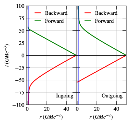
Figure 1: Comparison of photon trajectories through the Schwarzschild metric integrated both forwards (top) and backwards (bottom) in time, in both ingoing (left) and outgoing (right) Cartesian KS coordinates. In all panels the vertical blue line denotes the location of the event horizon. The ingoing Cartesian KS coordinates are horizon-penetrating for forward integration, whereas the outgoing Cartesian KS coordinates are horizon-penetrating for backward integration.

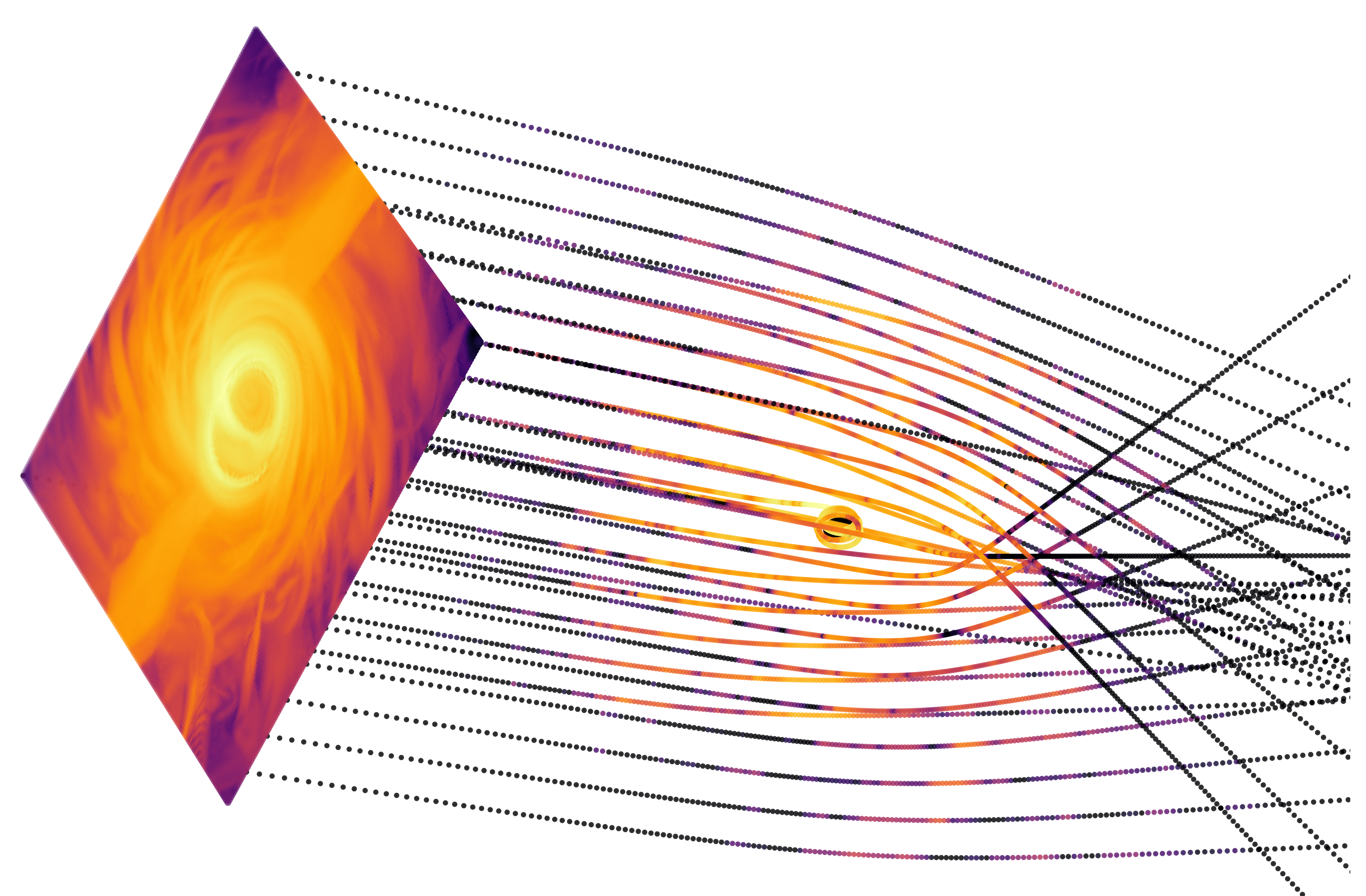
Figure 2: A visual representation of how Mahakala simulates the trajectories of photons from the observer’s image plane through the three dimensional space near a black hole. The image plane shows the resulting image with a logarithmic color scale. The color map along photon trajectories represents the total synchrotron emission at each point in the photon’s path through the output of a GRMHD simulation.

Most existing ray-tracing algorithms use either Boyer-Lindquist (BL) coordinates or spherical Kerr-Schild coordinates (see e.g., Noble et al. 2007; Psaltis & Johannsen 2012; Pu et al. 2016; Dexter 2016). However, the coordinate singularity at the pole ($\theta=0,\,\pi$) can cause numerical errors. To avoid these issues, Mahakala uses the Cartesian Kerr-Schild (KS) coordinate system. This choice of coordinates also allows us to seamlessly interface with the new AthenaK code (J. Stone et al. in preparation). In Cartesian KS coordinates, the Kerr metric is given by (see e.g., Visser 2007)

$$g_{\alpha\beta}=\eta_{\alpha\beta}+fl_{\alpha}l_{\beta},$$ (1)

where $\eta_{\alpha\beta}$ = $\mathrm{diag}(-1,1,1,1)$ is the Minkowski metric, $f$ is given by

$$f=\frac{2Mr^{3}}{r^{4}+a^{2}z^{2}},$$ (2)

and

$$l_{\alpha}=\left(\pm 1,\frac{rx+ay}{r^{2}+a^{2}},\frac{ry-ax}{r^{2}+a^{2}},\frac{z}{r}\right).$$ (3)

Here $M$ is the mass of the black hole, $a$ is the black hole spin parameter (i.e. the angular momentum of the black hole, with dimension $M$) and $r$ is defined implicitly as

$$x^{2}+y^{2}+z^{2}=r^{2}+a^{2}(1-z^{2}/r^{2}).$$ (4)

Throughout the paper we use the $\mathrm{(}-1,1,1,1)$ metric signature and set $c=G=1$ unless otherwise stated, where $G$ is the gravitational constant, and $c$ is the speed of light. In the above equations, the Greek indices vary from 0 to 3. The positive and negative signs in the $0$-th component of $l_{\alpha}$ correspond to the ingoing and outgoing Cartesian KS coordinates, respectively. In Figure 1, we compare the trajectories of photons through the Schwarzschild metric in both ingoing and outgoing Cartesian KS coordinates. As shown in the figure, photon trajectories integrated forwards in time in ingoing Cartesian KS coordinates are horizon-penetrating, while trajectories integrated backwards in time approach the horizon asymptotically. For outgoing Cartesian KS coordinates, the opposite is true; photon trajectories are only horizon-penetrating if they are evolved backwards in time (see G. Bozzola et al. in preparation for a detailed comparison of ingoing and outgoing KS coordinates). This result also holds for ingoing and outgoing spherical KS coordinates.

Mahakala can be used with both ingoing and outgoing Cartesian KS coordinates and integrates the photon trajectories backwards in time from the observer’s image plane into the regions near the black hole. By default, Mahakala uses the (non-horizon-penetrating) ingoing coordinates for consistency with the new AthenaK GRMHD code.

We follow the formalism of Johannsen & Psaltis (2010) and initialize the observer’s image plane at a distance $d$ from the black hole and at an inclination angle $i$ with respect to the black hole’s spin axis (see Figure 1 in Johannsen & Psaltis 2010). In Figure 2 we show an example simulated image along with selected photon trajectories used to generate the image. We define $x^{\prime}$ and $y^{\prime}$ as the coordinates on the image plane and relate them to the Carterian KS coordinates ($x,\,y,\,z$) as follows:

$$x=-y^{\prime}\cos i+d\sin i,$$ (5)

$$y=x^{\prime},$$ (6)

$$z=y^{\prime}\sin i+d\cos i.$$ (7)

We initialize a photon at each pixel location such that the direction of its momentum is parallel to the vector connecting the center of the black hole to the center of the image plane. We normalize the photon’s 4-momentum ($k$) such that $k^{0}=1$ and $k_{\mu}k^{\mu}=0$. We assume that the image plane is initialized at a large enough distance away from the black hole that the spacetime where the photons are initialized can be approximated as Minkowski.

The geodesic equations in curved space-time are

$$\frac{dx^{\mu}}{d\lambda}=k^{\mu},$$ (8a)

$$\frac{dk^{\mu}}{d\lambda}=-\Gamma^{\mu}_{\alpha\beta}k^{\alpha}k^{\beta},$$ (8b)

where $\lambda$ is an affine parameter and $\Gamma^{\mu}_{\alpha\beta}$ are the Christoffel symbols. We follow Chan et al. (2018) and re-write equation (8b) in terms of the metric derivative tensor,

$$\ddot{x}^{\mu}=-\left(g^{\mu\beta}\dot{x}^{\alpha}-\frac{1}{2}g^{\mu\alpha}\dot{x}^{\beta}\right)g_{\beta\gamma,\alpha}\dot{x}^{\gamma},$$ (9)

where $\dot{x}^{\mu}\equiv dx^{\mu}/d\lambda$. In this form, the operation count of calculating the geodesic equation is significantly reduced, resulting in higher efficiency. We numerically integrate the geodesic equation backwards in time using a Runge-Kutta $4^{th}$ order (RK4) scheme.

Most existing ray-tracing codes integrate the geodesic equation with respect to the affine parameter. However, using the affine parameter to integrate backwards in time through ingoing KS coordinates can cause significant errors near the horizon, due to the exponential growth of $k^{0}\equiv dt/d\lambda$ (see G. Bozzola et al. in preparation). Because of this, we include in Mahakala the ability to integrate in either affine parameter or coordinate time, which avoids these errors. The geodesic equation in coordinate time can be written as

$$\frac{dv^{i}}{dt}=-\Gamma^{i}_{\alpha\beta}v^{\alpha}v^{\beta}+\Gamma^{0}_{\alpha\beta}v^{\alpha}v^{\beta}v^{i},$$ (10)

where $v^{i}\equiv dx^{i}/dt$ and $v^{0}=1$. We again re-write the equation in terms of the metric derivative tensor

$$\frac{dv^{i}}{dt}=-\left(g^{{}^{\prime}i\beta}v^{\alpha}-\frac{1}{2}g^{{}^{\prime}i\alpha}v^{\beta}\right)g_{\beta\gamma,\alpha}v^{\gamma},$$ (11)

where $g^{{}^{\prime}i\mu}\equiv g^{i\mu}-v^{i}g^{0\mu}$. Mahakala integrates with respect to affine parameter by default.

We use a semi-adaptive time-step for integration, where the step-size depends on the photon’s location. The step-size $\mathcal{S}$ at iteration $i+1$ is given by

$$\mathcal{S}_{i+1}=\frac{r_{i}}{\mathcal{C}},$$ (12)

where $r_{i}$ is the radial distance of the photon from the center of the black hole for the $i$-th iteration and $\mathcal{C}$ is a free parameter that scales the step size. Mahakala does not explicitly use constants of motion to integrate the geodesic equation. Because of this, $k_{\mu}k^{\mu}\equiv k^{2}$ is unconstrained and is therefore a good measure of the numerical error. Figure 3 shows $|k_{\mu}k^{\mu}|$ as a function of time for different values of $\mathcal{C}$. As we increase the value of $\mathcal{C}$ from 20 to 50, the error decreases significantly from $\sim 10^{-8}$ to $\sim 10^{-10}$. Since increasing $\mathcal{C}$ further has a relatively small effect on the error and to ensure computational efficiency, we set $\mathcal{C}=50$ by default.

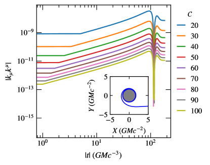
Figure 3: The value of $|k_{\mu}k^{\mu}|$, which is a measure of the error as a function of coordinate time for an example photon. Different colors correspond to different values of $\mathcal{C}$, and the inset shows the trajectory of the photon around a black hole with $a=0.9\,M$. For efficiency, we choose $\mathcal{C}=50$ as the default value, but the user may specify a higher value if a smaller error is required.

Equations (10) and (11) are only valid where $dt/d{\lambda}$ is finite and well-defined. For integration backwards in time in ingoing Cartesian KS coordinates, $dt/d\lambda$ grows exponentially near the horizon and becomes infinite at the horizon. To avoid this, Mahakala stops the integration for photons that fall within a distance of $\epsilon=10^{-4}\,M$ from the horizon. We also stop integrating the photons that reach distances larger than $d$, the distance between the black hole and the image plane.

3 Synthetic Images of GRMHD Simulations

Our primary goal with Mahakala is to simulate the mm-wavelength emission of low-luminosity accretion flows such as the ones onto Sgr A^∗ and the supermassive black hole in M87. Mahakala calculates synchrotron emissivity since it is the primary emission mechanism for these sources at these wavelengths (see, e.g., Genzel et al. 2010). To demonstrate Mahakala’s capabilities, we simulate 1.3 mm images of snapshots from GRMHD simulations performed with the new AthenaK code (J. Stone et al. in preparation). As a proof of concept, we use a uniform Cartesian grid and linearly interpolate between grid points to calculate the values of the primitive variables (the variables natively recorded by the GRMHD simulations) along geodesic trajectories. Since the effects of radiation on the dynamics of the flow are expected to be negligible for M87 and Sgr A*, we use GRMHD simulations that do not incorporate the effects of radiation pressure or radiative cooling. We also assume that the GRMHD flow does not change in the time it takes for the photon trajectories to evolve, i.e. we use the fast-light approximation.

The primitive variables of the AthenaK simulations are the fluid-frame density $\rho$, fluid-frame gas pressure $p_{\text{gas}}$, spatial components of the fluid velocity in the normal-frame $u^{\prime i}$, and the spatial components of the magnetic field in Cartesian coordinate frame $B^{i}$. The contravariant components of the fluid magnetic field in the coordinate frame ($b^{\mu}$) are given by (see, e.g., White et al. 2016; Stone et al. 2020)

$$b^{0}=u_{i}B^{i},$$ (13a)

$$b^{i}=\frac{1}{u^{0}}(B^{i}+b^{0}u^{i}),$$ (13b)

where $u^{0}=\gamma/\alpha$, $u^{i}=u^{\prime i}-\beta^{i}\gamma/\alpha$, $\alpha=(-g^{00})^{-1/2}$ is the lapse, $\beta^{i}=\alpha^{2}g^{0i}$ is the shift, and

$$\gamma=(1+g_{ij}u^{\prime i}u^{\prime j})^{1/2}$$ (14)

is the Lorentz factor in the normal frame. We denote the contravariant components of the fluid velocity in the coordinate frame as $u^{\mu}$ throughout. We interpolate the primitive variables rather than $u^{\mu}$ and $b^{\mu}$ to ensure that $u_{\mu}u^{\mu}=-1$ and $u_{\mu}b^{\mu}=0$ along the geodesic trajectories.

3.1 Radiative Transfer

Accounting for emission and absorption, the covariant form of the general relativistic radiative transfer equation (for total intensity and neglecting scattering) is (see, e.g., Younsi et al. 2012)

$$\frac{d\mathcal{I}}{d\lambda}=-k^{\mu}u_{\mu}\left(-\alpha_{\nu,0}\mathcal{I}+\frac{j_{\nu,0}}{\nu^{3}}\right).$$ (15)

Here $\mathcal{I}=I_{\nu}/\nu^{3}$ is Lorenz-invariant and $I_{\nu}$ is the specific intensity of the ray at frequency $\nu$. In the above equation, $\alpha_{\nu}$ and $j_{\nu}$ correspond to the absorption and synchrotron emissivity at frequency $\nu$, respectively. Quantities with subscript $0$ are evaluated in the local frame of the plasma. The frequency of radiation measured by the observer is

$$\nu=-k^{\mu}u_{\mu},$$ (16)

where $k^{\mu}$ is the contravariant 4-momentum of the photon and $u_{\mu}$ is the covariant plasma four-velocity.

The modular nature of Mahakala allows us to calculate the radiative transfer equation (15) either simultaneously with the geodesic equation (10) or in a separate step. Performing each step separately results in significant speed up in use cases where the geodesics remain the same for several images, such as when simulating several snapshots within a simulation or when varying parameters that only affect the radiative transfer (e.g., $n_{e}$, $\mathcal{M}$, and $R_{\mathrm{high}}$ defined below). However, if the user would like to vary parameters that affect the geodesic trajectories (e.g., $i$, and $a$) then solving the geodesics and the radiative transfer equations simultaneously will be more efficient.

As discussed in section 2, Mahakala can integrate the geodesic equation with respect to either the affine parameter or coordinate time. To solve the radiation transfer equation when integrating in coordinate time, we can use the chain rule to write equation (15) as

$$\frac{d\mathcal{I}}{dt}=-k^{\mu}u_{\mu}\left(-\alpha_{\nu,0}\mathcal{I}+\frac{j_{\nu,0}}{\nu^{3}}\right)\kappa,$$ (17)

where $\kappa=d\lambda/dt$. We calculate $\kappa$ by solving the following pair of coupled differential equations

$$\frac{d\lambda}{dt}=\kappa,$$ (18)

$$\frac{d\kappa}{dt}=\kappa\Gamma^{0}_{\alpha\beta}v^{\alpha}v^{\beta},$$ (19)

where $v^{\mu}=dx^{\mu}/dt$. We decrease the computational expense of solving equation (19) by writing it in terms of the metric derivative tensor as done for equation (9).

3.2 Emissivity

We restore $c$ throughout section  3.2. We adopt the following approximate expression for thermal synchrotron emissivity (Leung et al. 2011)

$$j_{\nu}=n_{e}\frac{\sqrt{2}\pi e^{2}\nu_{s}}{3K_{2}(1/\Theta_{e})c}(X^{1/2}+2^{11/12}X^{1/6})^{2}\exp{(-X^{1/3})}.$$ (20)

Here $e$ is the electron charge, $n_{e}$ is the electron density, and $K_{2}$ is the modified Bessel function of the second kind for integer order 2. $X$ is given by

$$X=\frac{\nu}{\nu_{s}},$$ (21)

where $\nu_{s}=(2/9)\nu_{c}\Theta_{e}^{2}\sin\theta_{B}$, and the cyclotron frequency ($\nu_{c}$) is given by

$$\nu_{c}=\frac{eB}{2\pi m_{e}c}.$$ (22)

The pitch angle ($\theta_{B}$) is the angle between the emitted or absorbed photon and the magnetic field vector $B$ as evaluated in the fluid frame

$$\cos\theta_{B}=\frac{k_{\mu}b^{\mu}}{-k_{\mu}u^{\mu}\sqrt{b_{\mu}b^{\mu}}}.$$ (23)

The dimensionless electron temperature is

$$\Theta_{e}\equiv\frac{kT_{e}}{m_{e}c^{2}},$$ (24)

where $k$ is the Boltzmann constant, $T_{e}$ is the electron temperature, and $m_{e}$ is the mass of the electron. We calculate the absorption coefficient using Kirchoff’s Law (see, e.g., chapter 1 of Rybicki & Lightman 1986).

Low-luminosity accreting black holes, such as the black hole in M87 and Sgr A^∗, are expected to have advection dominated accretion flows (ADAFs; see, e.g., Narayan et al. 1998 for a review). Due to their low accretion rates, ADAFs have such low densities that they are effectively Coulomb collisionless. As a result, their ions and electrons may not reach thermal equilibrium, thus producing a two-temperature plasma (see, e.g., Quataert 1999; Quataert & Gruzinov 1999). Despite this, many currently available GRMHD simulations only evolve a single plasma temperature or internal energy (although see e.g., Ressler et al. 2015; Chael et al. 2019). To recover the electron temperature from the GRMHD variables, we set the electron-to-ion temperature ratio ($T_{i}/T_{e}$) based on the local ratio of gas to magnetic pressure in the plasma, $\beta=p_{\text{gas}}/p_{\text{mag}}$, as follows (see, e.g., Mościbrodzka et al. 2016; Event Horizon Telescope Collaboration et al. 2019a),

$$\frac{T_{i}}{T_{e}}=R_{\mathrm{high}}\frac{\beta^{2}}{1+\beta^{2}}+\frac{1}{1+\beta^{2}},$$ (25)

where $R_{\mathrm{high}}$ is a free parameter. Following Wong et al. (2022), we do not set the ion temperature equal to the fluid (gas) temperature to avoid overcounting the energy in the system. Instead, we calculate $T_{e}$ using the total fluid internal energy,

$$T_{e}=\frac{m_{p}u(\hat{\gamma_{e}}-1)(\hat{\gamma_{i}}-1)}{k\rho((\hat{\gamma_{i}}-1)y+(\hat{\gamma_{e}}-1)Rz)},$$ (26)

where $m_{p}$ is the proton mass and $u$ is the internal energy. Here $1/y$ and $1/z$ correspond to the total number of electrons and nucleons per atom, with $y=z=1$ for pure hydrogen. We set the adiabatic index for the ions to $\hat{\gamma_{i}}=5/3$ since they are typically non-relativistic and $\hat{\gamma_{e}}=4/3$ for the typically relativistic electrons.

4 Tests from the Literature

In this section we ensure the accuracy of Mahakala by performing several tests from the literature. Most tests included in this section are reproduced from Gold et al. (2020) where a large number of radiative ray-tracing codes were compared to each other.

4.1 Null Geodesic Deflection

We begin with a test of how the azimuthal deflection angle of null geodesic trajectories ($\Delta\phi$) depends on the impact parameter $b$ (Gold et al., 2020). Analytic solutions for the deflection angle of null geodesics confined to the $x-y$ plane in the Kerr metric can be obtained by a quadrature of standard, elliptic functions given in Iyer & Hansen (2009). For this test, we uniformly vary the impact parameter $b$ from $-20\,M$ to $20\,M$ in intervals of $0.4\,M$. We ignore photons with impact parameter satisfying $b_{-}\leq b\leq b_{+}$ as these photons fall inside the black hole. Here, $b_{-}$ and $b_{+}$ are given by

$$b_{\pm}=-a+6M\cos{\bigg{(}\frac{1}{3}\cos^{-1}\bigg{(}\mp\frac{a}{M}\bigg{)}\bigg{)}}.$$ (27)

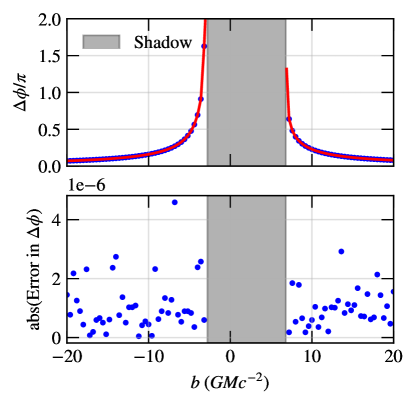
Figure 4: (top) Deflection angle of null geodesics in the equatorial plane around a black hole with $a=0.9\,M$ integrated with Mahakala, as a function of the impact parameter $b$. (bottom) The absolute error, as compared to analytic solutions, in the deflection angle calculated by Mahakala.

We show that the numerical and analytic results are in good agreement in Figure 4, where we have set the black hole spin parameter to $a=0.9\,M$ and the distance of the black hole from the observer’s image plane to $d=1000\,M$. The absolute error between the numerical and analytical results (lower panel of Figure 4) is of the order of $~{}10^{-6}$. Our range of errors is consistent with the other codes included in Gold et al. (2020).

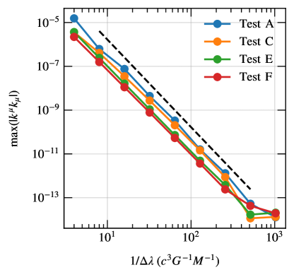
Figure 5: Maximum error, $\mathrm{max}(|k\cdot k|)$, as a function of the inverse of step size, $1/\Delta\lambda$, for the four spherical orbit tests shown in Figure 6. We vary the step size from $1/4\,M$ to $1/1024\,M$ in factors of two. Mahakala’s integration scheme converges at 4–th order, i.e., $y\sim x^{-4}$ (black dashed line) as expected for an RK4 method.

4.2 Unstable Spherical Photon Orbits

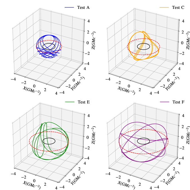
Figure 6: Unstable spherical photon orbits around a black hole with spin $a=M$ and time step $\Delta\lambda=1/1024\,M$. For all panels, solid colored lines are the photon orbits, black solid circles are the (physical) singularities, and red dashed circles mark the radii of the spherical orbits on the equatorial planes. All orbits start by moving upward from the positive x-sides of the red dashed circles, and are integrated forwards in time for a fixed number of iterations.

Here we test the accuracy of Mahakala’s RK4 geodesic integration with convergence tests for unstable spherical photon orbits (see, e.g., Chan et al. 2018). Integration of spherical photon orbits allows us to test the long term behavior of our algorithm since the errors will accumulate along these trajectories. We set $a=M$ and use a constant time-step for this test.

For a black hole with mass $M$ and spin $a$, spherical photon orbits will lie between the prograde radius ($r_{p}$), and the retrograde radius ($r_{r}$),

$$r_{p}\equiv 2M\bigg{\{}1+\cos\bigg{[}\frac{2}{3}\cos^{-1}\bigg{(}-\frac{|a|}{M}\bigg{)}\bigg{]}\bigg{\}},$$ (28)

$$r_{r}\equiv 2M\bigg{\{}1+\cos\bigg{[}\frac{2}{3}\cos^{-1}\bigg{(}\frac{|a|}{M}\bigg{)}\bigg{]}\bigg{\}},$$ (29)

where $r_{p}$ and $r_{r}$ also satisfy the inequality $M\leq r_{p}\leq 3M\leq r_{r}\leq 4M$. Mahakala then calculates the normalized angular momentum ($\Phi$) and the Carter constant ($Q$), used to define the initial conditions of the photons (see, e.g., Teo 2003),

$$\Phi=-\frac{r^{3}-3Mr^{2}+a^{2}r+a^{2}M}{a(r-M)},$$ (30)

$$Q=-\frac{r^{3}(r^{3}-6Mr^{2}+9M^{2}r-4a^{2}M)}{a^{2}(r-M)^{2}}.$$ (31)

In Figure 5 we demonstrate that Mahakala converges as expected for RK4 integration with convergence plots for the four spherical photon orbits we consider from Chan et al. (2018). As we decrease our step size from $1/4\,M$ to $1/1024\,M$ in factors of two, the maximum error along the trajectory, $\mathrm{max}(|k_{\mu}k^{\mu}|)$, decreases as expected for a 4–th order scheme. Figure 6 shows the results of simulating these trajectories with Mahakala. The photon trajectories remain stable for several orbits and are consistent with the results of Chan et al. (2018).

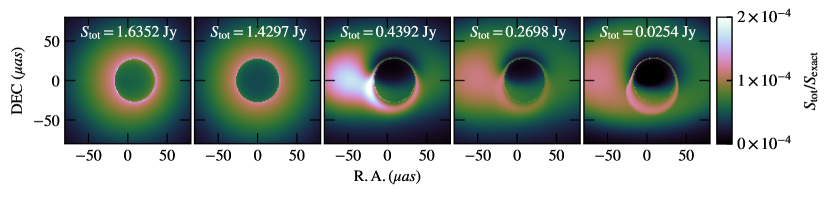
Figure 7: Images produced by Mahakala for the five parameterized models in Gold et al. (2020). The image morphology and total flux are consistent with the results of the several radiative ray-tracing algorithms in Gold et al. (2020).

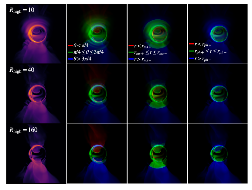
Figure 8: (first column) Example 1.3 mm image simulated with Mahakala for a snapshot from a SANE GRMHD simulation with spin $a=0.9\,M$, inclination $i=60^{\circ}$, electron temperature prescription set by $R_{\mathrm{high}}=10,\,40,\,\mathrm{and}\,160$ (top, middle, and bottom rows respectively, for all columns), and a mass density scale of $\mathcal{M}=1\times 10^{27}$. (second column) The same snapshot as the first column but here the different colors correspond to different regions in the 3-D flow volume where the emission originates. Red denotes emission from the forward jet, defined here as a conical shell where $\theta<\pi/4$. Green denotes emission from the disk region within $\pi/4\leq\theta\leq 3\pi/4$ and blue denotes the counter jet with $\theta>3\pi/4$. To calculate the color of each pixel we calculate the relative fraction of the specific intensity at that pixel that was emitted from each region. The third and fourth columns show 3-color images where each color corresponds to a spherical shell in 3-D flow space. We define $r_{ms\pm}$ and $r_{ph\pm}$ as the innermost stable circular orbit (ISCO) and photon orbit respectively (see, e.g., Bardeen et al. 1972), where $+$ corresponds to the prograde orbits and $-$ corresponds to the retrograde orbits. For spin $a=0.9\,M$, the prograde and retrograde ISCO are at 2.321 $M$ and 8.717 $M$ respectively, and prograde and retrograde photon orbits are at 1.558 $M$ and 3.910 $M$ respectively. We use a gamma scale for all panels with $\Gamma=0.1$ (i.e. the colors show intensity to the $\Gamma$ power).

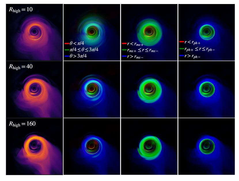
Figure 9: Same as Figure 8 but with $i=17^{\circ}$.

4.3 Images from Analytic Models

We test the radiative transfer components of Mahakala by reproducing the analytic image test described in section 3.2 of Gold et al. (2020). The test comprises an analytic accretion model simulated without the effects of scattering or polarization. We repeat this test with the same initial parameters, camera position, and parameter values as in Gold et al. (2020, see their Table 1 for parameter values). We show the resulting images in Figure 7. The image morphology and total flux values are consistent with those of Gold et al. (2020, see their Table 2 for total flux values).

5 Applications

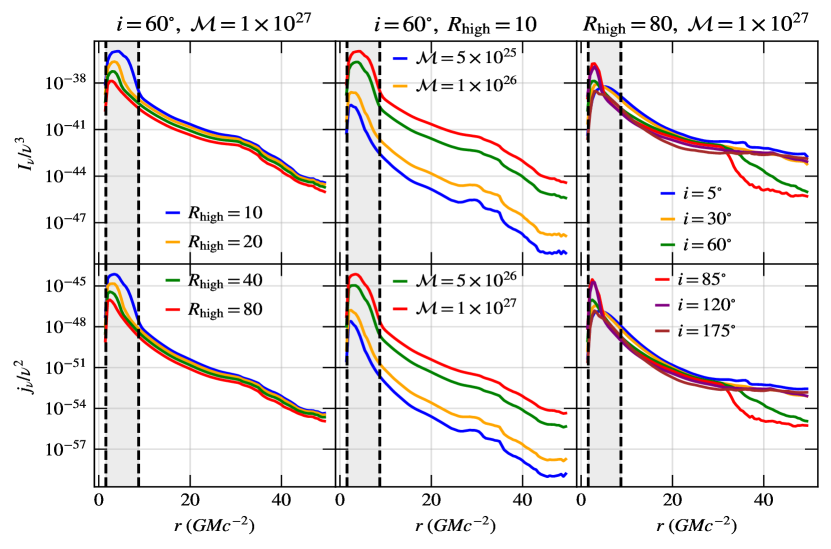
Figure 10: Average specific intensity (top row) and invariant synchrotron emission (bottom row) as a function of radius. In the left panels we vary $R_{\mathrm{high}}$ and set $\mathcal{M}=1\times 10^{27}$ and $i=60^{\circ}$. In the middle panels we vary $\mathcal{M}$ and set $R_{\mathrm{high}}=10$ and $i=60^{\circ}$. In the right panels we vary $i$ and set $R_{\mathrm{high}}=80$ and $\mathcal{M}=1\times 10^{27}$. In all cases most of the emission originates within $\sim 10\,M$. The dashed lines correspond to the retrograde ISCO ($8.717\,M$) and the prograde photon orbit ($1.558\,M$). Here and in the following figure we set the black hole spin parameter to $a=0.9\,M$ and the black hole mass to $M=6.5\times 10^{9}M_{\odot}$.

We use Mahakala to simulate 1.3 mm images of GRMHD outputs generated by the new AthenaK code (J. Stone et al. in preparation). As a proof of concept, we use a single low-resolution, uniform Cartesian grid GRMHD simulation with spin $a=0.9\,M$ and initial conditions that result in low magnetic flux near the horizon, commonly referred to as the standard and normal evolution state (SANE, see, e.g., Igumenshchev et al. 2003). We simulate images of 300 GRMHD snapshots with a time resolution of $50\,M$. Throughout this section we use ray-traced images with a field of view of $64\,M$ and an image resolution such that the pixel side length is $1/8\,M$ (see Psaltis et al. 2020b for an exploration of the effects of resolution in simulated images).

The results of GRMHD simulations are invariant under rescaling of both length and mass. However, the radiative transfer equations do depend on the black hole’s mass (which sets the length scale of the simulation) and the flow’s mass density scale. We set the black hole mass to $M=6.5\times 10^{9}M_{\odot}$ throughout, for consistency with the supermassive black hole in M87 (see Gebhardt et al. 2011; Event Horizon Telescope Collaboration et al. 2019f) and parameterize the density scale normalization as $\mathcal{M}/\mathcal{L}^{3}$, where $\mathcal{L}=GMc^{-2}$ is the length scale (where we have restored the gravitational constant and the speed of light for clarity, see also Wong et al. 2022). The units of $\mathcal{M}$ are such that multiplying the density in the fluid simulation by $\mathcal{M}/\mathcal{L}^{3}$ yields a value with units of g/cm³. However, for simplicity, we will not include units when quoting values of $\mathcal{M}$, as they ultimately depend upon the code units used in the fluid simulation. We use the mass density scale to determine physical units for the total electron density, internal energy, and magnetic field strength. In contrast to the simulation library included in Event Horizon Telescope Collaboration et al. (2019e, 2022e), we do not use the total flux at 1.3 mm to set the mass scale $\mathcal{M}$, but rather vary it independently from the other free parameters. This allows us to explore the effect of the mass density independently from other variables.

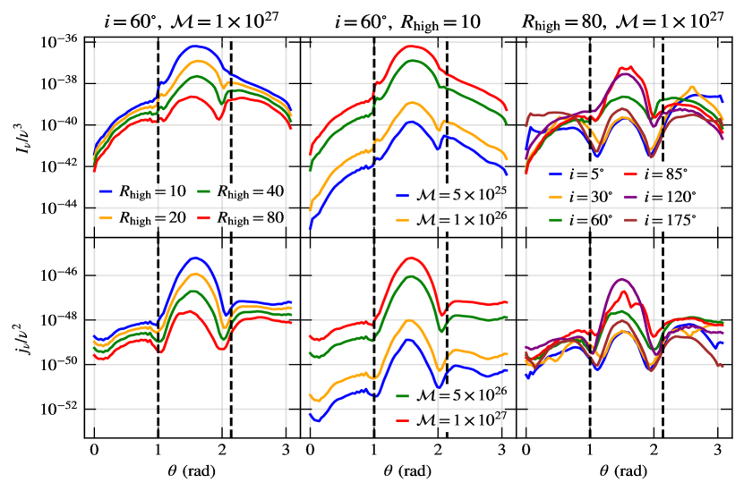
Figure 11: Same as Figure 10 but as a function of $\theta$. In most cases, the disk has the largest contribution to the image, but for high $R_{\mathrm{high}}$ the counter jet can contribute more than the disk. The counter jet usually contributes more than the forward jet, although the relative contributions are similar. The dashed lines represent 1 radian ($\approx 57.3^{\circ}$) from the polar axis that is nearest and farthest from the observer.

Mahakala is written with flexibility and ease of use as a high priority. This flexibility allows us to easily explore how different regions in the flow are related to image features. As an example, we calculate the relative contribution of different regions in the flow of example snapshot in Figure 8. The first column on the left shows a single GRMHD snapshot imaged at 60 degree inclination for three values of $R_{\mathrm{high}}$. The second column shows three-color images, with each color corresponding to emission from a different region in space near the black hole. Emission that originates in regions where $\theta<\pi/4$ (forward jet) is shown in red, emission from regions where $\pi/4\leq\theta\leq 3\pi/4$ (the disk) is shown in green, and emission from regions where $\theta>3\pi/4$ (counter jet) is shown in blue. We note that for each color, we ignore the absorption in regions composite to the trial emission region. Not surprisingly, for all values of $R_{\mathrm{high}}$, the disk region contributes the most to the central region of the image, while the forward and counter jets contribute to emission above and below the central ring. As $R_{\mathrm{high}}$ is increased, the relative contribution of the disk region decreases and the forward and counter jet become more visible.

The third column also shows three color images, but with different colors corresponding to the region within the prograde ISCO radius (red), between the prograde and retrograde ISCO radius (green), and outside of the retrograde ISCO radius (blue). For all values of $R_{\mathrm{high}}$, the region between the prograde and retrograde ISCO radii contributes the most to the image and dominates the ring-like feature. A small amount of emission originates from within the prograde radius. The region outside of the retrograde ISCO radius contributes to the jet features seen towards the north and south of the images. The fourth column is similar to the third but for the prograde and retrograde photon orbit radii. The region outside of the retrograde photon orbit contributes to the extended jet features while most of the central ring-like emission originates between the prograde and retrograde photon orbits. Negligible emission originates from within the photon orbit.

Figure 9 is similar to Figure 8 but for an inclination angle of 17 degrees, consistent with the inclination angle of the large scale jet of M87 observed at radio frequencies (Walker et al., 2018). At this inclination the forward jet contributes the most for $R_{\mathrm{high}}=10$ but the counter jet contributes the most for the higher values of $R_{\mathrm{high}}$. Like the higher-inclination images, most of the emission originates from between the prograde and retrograde ISCO orbits for all values of $R_{\mathrm{high}}$. The extended emission seen towards the bottom right of the images is emitted farther from the black hole. The region within the prograde ISCO orbit contributes a small amount of emission within the central brightness depression. the main ring feature and the emission within the ring originate from inside the retrograde photon orbit, while the emission external to the bright ring is dominated by emission that originates outside of the retrograde photon orbit. Although the example here is for a single GRMHD snapshot, it demonstrates Mahakala’s flexibility, and shows how easily we can explore the contribution of different flow regions.

To further explore the behavior in Figures 8 and 9, we calculate the image contribution of spherical shells in the 3-dimensional GRMHD simulation volume. In the bottom-left panel of Figure 10 we calculate the average invariant synchrotron emission ($j_{\nu}/\nu^{2}$) within spherical shells of width $0.5\,M$ as a function of the mean shell radius for several values of $R_{\mathrm{high}}$. Increasing the value of $R_{\mathrm{high}}$ results in an overall decrease of $j_{\nu}/\nu^{2}$. If we ignore absorption, the emissivity peaks close to the black hole and decreases monotonically at larger radii (peaks between $r\approx 2.7\,M$ and $r\approx 3.7\,M$ for different $R_{\mathrm{high}}$).

To explore the effects of absorption, we also plot the specific intensity $I_{\nu}/\nu^{3}$ in the top left panel of Figure 10. The mass scale used in this example is low enough that the disk is optically thin at 1.3 mm. Because of this, the radial dependence of $j_{\nu}/\nu^{2}$ and $I_{\nu}/\nu^{3}$ are similar. Note, however, that in this example we ignore all effects of matter outside each shell, i.e. the effect of absorption outside of each shell is not included in the calculation of the average specific intensity for the shell. This approximation is justified since the low densities result in low absorption.

The middle panels of Figure 10 are similar to the left panels, but the different curves correspond to different values of $\mathcal{M}$. For these panels we have set $R_{\mathrm{high}}=10$ and $i=60^{\circ}$. Even for higher values of $\mathcal{M}$, absorption has a relatively small effect and the emission peaks very close to the black hole (between $r\approx 2.2\,M$ and $r\approx 3.7\,M$). We explore the effect of the inclination angle in the right panels of Figure 10, where we set $R_{\mathrm{high}}=80$ and $\mathcal{M}=1\times 10^{27}$. For all values of $R_{\mathrm{high}}$, $\mathcal{M}$, and $i$ we consider, the majority of the emission in 1.3 mm images originates within $\sim 10\,M$ and peaks between $r\approx 2.7\,M$ and $r\approx 4.7\,M$. This is consistent with previous expectations and provides additional certainty that the 1.3 mm images of M87 and Sgr A^∗ probe the region very close to the black hole, as has previously been argued (see, e.g., Event Horizon Telescope Collaboration et al. 2019e; Wong et al. 2022).

Similar to the exploration of radial dependence described above, we also explore the dependence on $\theta$. We divide the 3-D flow volume into 90 hollow cones, each with a theta range of $\pi/90$. We calculate the average values of $j_{\nu}/\nu^{2}$ and $I_{\nu}/\nu^{3}$ for all GRMHD snapshots in each cone, ignoring the absorption of matter outside each cone. Figure 11 shows the average emissivity and specific intensity in each cone as a function of the mean $\theta$ of the cone. In the left panels, the emissivity and specific intensity both peak at $\theta\approx\pi/2$, i.e., the disk region, for most values of $R_{\mathrm{high}}$. However, as $R_{\mathrm{high}}$ increases, the disk contributes to the total flux relatively less when compared to the counter-jet. At $R_{\mathrm{high}}=80$, the peak contribution to $I_{\nu}/\nu^{3}$ is from the counter-jet. We explore the effects of $\mathcal{M}$ in the middle panels where we again set $i=60^{\circ}$ and $R_{\mathrm{high}}=10$. Although the mass scale affects the overall magnitude of the emissivity and specific intensity, it has a negligible effect on the trends as a function of $\theta$. We explore the effect of inclination angle in the right panels of Figure 11. In all cases, the forward jet contributes less to the emissivity and specific intensity than the counter jet, and the disk dominates in most regions of the parameter space explore here. This is consistent with the results of Event Horizon Telescope Collaboration et al. (2019e, see their Figure 11), though in that case $R_{\mathrm{high}}=160$.

The exploration we performed in this section only required running the ray-tracing six times, one for each inclination angle shown in Figure 10 and 11. Over 4,000 simulated images were used for the averages shown in the figures (300 snapshots in time and 14 parameter combinations). Once we compute the trajectory information, the radiative transfer calculations are vectorized in Python with numpy and are thus very efficient.

6 Summary

We present Mahakala, a new, Python based, modular ray-tracing and radiation transfer code for arbitrary space-times. Mahakala uses Google’s new machine learning framework, JAX, which runs in parallel on CPUs, GPUs, and TPUs. JAX performs accelerated automatic differentiation, allowing the user to efficiently simulate geodesic trajectories through arbitrary space-times without the need to manually calculate Christoffel symbols. Mahakala has been developed to simulate the mm-wavelength radiation of low-luminosity accreting supermassive black holes and calculates synchrotron emission and absorption. We use Cartesian KS coordinates to avoid numerical issues near the pole of spherical coordinates, and we can integrate photon trajectories with respect to coordinate time or affine parameter. Mahakala natively supports the new GPU-accelerated AthenaK GRMHD code, which also uses Cartesian KS coordinates.

We verify both the radiative transfer and geodesic integration components of Mahakala with tests from the literature (see Section 4). We show that the errors in the deflection angle of null trajectories near a Kerr black hole are in the range of other radiative transfer codes explored in Gold et al. (2020). We perform convergence tests with spherical photon orbits and show that Mahakala converges as expected for a fourth order scheme (see also Chan et al. 2018). Finally, we test the radiative transfer component of Mahakala with analytic accretion model tests from Gold et al. (2020). The image morphology and total flux are consistent with the results of several radiative ray-tracing algorithms that are compared in Gold et al. (2020).

One of the main aims of Mahakala is flexibility and ease of use. Since Mahakala can easily be run in a Python jupyter notebook, we also hope that it will remove the barrier to entry for radiative ray-tracing simulations. The modular nature of Mahakala allows us to explore in detail how different regions of the 3-D GRMHD flow volume contribute to image features. We demonstrate this with an example SANE GRMHD simulation with spin $a=0.9\,M$ generated by AthenaK. We show in Section 5 that the majority of emission at 1.3 mm comes from within $\sim 10\,M$ of the black hole with a peak at $\sim 3\,M$. This result is robust to changes in the overall density scale ($\mathcal{M}$), the parameter that sets the electron temperature prescription ($R_{\mathrm{high}}$), and the observer’s inclination angle with respect to the black hole spin axis ($i$). This provides further evidence that the EHT images of M87 and Sgr A^∗ probe the regions close to their respective black holes and that most of the emission has been gravitationally lensed by the black holes.

In addition to the dependence on the emission radius, we also explore how conical shells at different $\theta$ contribute to the image. For our example SANE simulation, we find that the disk almost always contributes more emission to the image than the forward or counter jet. However, for high values of $R_{\mathrm{high}}$, the counter jet may contribute more to the total flux density than the disk. In all cases, we find that the forward jet never dominates the image. In future work, we will extend Mahakala to include polarization and allow for the fluid to evolve as light propagates through the domain (i.e. slow light).

References

- Bardeen (1973) Bardeen, J. M. 1973, in Black Holes (Les Astres Occlus), 215–239
- Bardeen et al. (1972) Bardeen, J. M., Press, W. H., & Teukolsky, S. A. 1972, ApJ, 178, 347
- Bradbury et al. (2018) Bradbury, J., Frostig, R., Hawkins, P., et al. 2018
- Bronzwaer et al. (2018) Bronzwaer, T., Davelaar, J., Younsi, Z., et al. 2018, A&A, 613, A2
- Bronzwaer et al. (2020) Bronzwaer, T., Younsi, Z., Davelaar, J., & Falcke, H. 2020, A&A, 641, A126
- Chael et al. (2019) Chael, A., Narayan, R., & Johnson, M. D. 2019, MNRAS, 486, 2873
- Chan et al. (2018) Chan, C.-k., Medeiros, L., Özel, F., & Psaltis, D. 2018, ApJ, 867, 59
- Chan et al. (2013) Chan, C.-k., Psaltis, D., & Özel, F. 2013, ApJ, 777, 13
- Chan et al. (2015) Chan, C.-k., Psaltis, D., Özel, F., et al. 2015, ApJ, 812, 103
- Christian & Chan (2021) Christian, P., & Chan, C.-k. 2021, ApJ, 909, 67
- Cunningham (1975) Cunningham, C. T. 1975, ApJ, 202, 788
- De Villiers & Hawley (2003) De Villiers, J.-P., & Hawley, J. F. 2003, ApJ, 589, 458
- Dexter (2016) Dexter, J. 2016, MNRAS, 462, 115
- Dexter & Agol (2009) Dexter, J., & Agol, E. 2009, ApJ, 696, 1616
- Dexter & Fragile (2011) Dexter, J., & Fragile, P. C. 2011, ApJ, 730, 36
- Dolence et al. (2009) Dolence, J. C., Gammie, C. F., Mościbrodzka, M., & Leung, P. K. 2009, ApJS, 184, 387
- Event Horizon Telescope Collaboration et al. (2019a) Event Horizon Telescope Collaboration, Akiyama, K., Alberdi, A., et al. 2019a, ApJ, 875, L1
- Event Horizon Telescope Collaboration et al. (2019b) —. 2019b, ApJ, 875, L2
- Event Horizon Telescope Collaboration et al. (2019c) —. 2019c, ApJ, 875, L3
- Event Horizon Telescope Collaboration et al. (2019d) —. 2019d, ApJ, 875, L4
- Event Horizon Telescope Collaboration et al. (2019e) Event Horizon Telescope Collaboration, Akiyama, K., Alberdi, A., et al. 2019e, The Astrophysical Journal Letters, 875, L5
- Event Horizon Telescope Collaboration et al. (2019f) Event Horizon Telescope Collaboration, Akiyama, K., Alberdi, A., et al. 2019f, ApJ, 875, L6
- Event Horizon Telescope Collaboration et al. (2021a) Event Horizon Telescope Collaboration, Akiyama, K., Algaba, J. C., et al. 2021a, ApJ, 910, L12
- Event Horizon Telescope Collaboration et al. (2021b) —. 2021b, ApJ, 910, L13
- Event Horizon Telescope Collaboration et al. (2022a) Event Horizon Telescope Collaboration, Akiyama, K., Alberdi, A., et al. 2022a, ApJ, 930, L12
- Event Horizon Telescope Collaboration et al. (2022b) —. 2022b, ApJ, 930, L13
- Event Horizon Telescope Collaboration et al. (2022c) —. 2022c, ApJ, 930, L14
- Event Horizon Telescope Collaboration et al. (2022d) —. 2022d, ApJ, 930, L15
- Event Horizon Telescope Collaboration et al. (2022e) Event Horizon Telescope Collaboration, Akiyama, K., Alberdi, A., et al. 2022e, The Astrophysical Journal Letters, 930, L16
- Event Horizon Telescope Collaboration et al. (2022f) Event Horizon Telescope Collaboration, Akiyama, K., Alberdi, A., et al. 2022f, ApJ, 930, L17
- Gammie et al. (2003) Gammie, C. F., McKinney, J. C., & Tóth, G. 2003, ApJ, 589, 444
- Gebhardt et al. (2011) Gebhardt, K., Adams, J., Richstone, D., et al. 2011, ApJ, 729, 119
- Genzel et al. (2010) Genzel, R., Eisenhauer, F., & Gillessen, S. 2010, Reviews of Modern Physics, 82, 3121
- Gold et al. (2020) Gold, R., Broderick, A. E., Younsi, Z., et al. 2020, ApJ, 897, 148
- Igumenshchev et al. (2003) Igumenshchev, I. V., Narayan, R., & Abramowicz, M. A. 2003, ApJ, 592, 1042
- Iyer & Hansen (2009) Iyer, S. V., & Hansen, E. C. 2009, Phys. Rev. D, 80, 124023
- Johannsen (2013) Johannsen, T. 2013, Phys. Rev. D, 87, 124017
- Johannsen & Psaltis (2010) Johannsen, T., & Psaltis, D. 2010, ApJ, 718, 446
- Karas et al. (1992) Karas, V., Vokrouhlicky, D., & Polnarev, A. G. 1992, MNRAS, 259, 569
- Kocherlakota et al. (2021) Kocherlakota, P., Rezzolla, L., Falcke, H., et al. 2021, Phys. Rev. D, 103, 104047
- Leung et al. (2011) Leung, P. K., Gammie, C. F., & Noble, S. C. 2011, ApJ, 737, 21
- Luminet (1979) Luminet, J. P. 1979, A&A, 75, 228
- Medeiros et al. (2017) Medeiros, L., Chan, C.-k., Özel, F., et al. 2017, ApJ, 844, 35
- Medeiros et al. (2018a) —. 2018a, ApJ, 856, 163
- Medeiros et al. (2018b) Medeiros, L., Lauer, T. R., Psaltis, D., & Özel, F. 2018b, ApJ, 864, 7
- Medeiros et al. (2020) Medeiros, L., Psaltis, D., & Özel, F. 2020, ApJ, 896, 7
- Mościbrodzka et al. (2016) Mościbrodzka, M., Falcke, H., & Shiokawa, H. 2016, A&A, 586, A38
- Mościbrodzka & Gammie (2018) Mościbrodzka, M., & Gammie, C. F. 2018, MNRAS, 475, 43
- Narayan et al. (1998) Narayan, R., Mahadevan, R., & Quataert, E. 1998, in Theory of Black Hole Accretion Disks, ed. M. A. Abramowicz, G. Björnsson, & J. E. Pringle, 148–182
- Noble et al. (2012) Noble, S. C., Gammie, C. F., McKinney, J. C., & Del Zanna, L. 2012, PVS-GRMHD: Conservative GRMHD Primitive Variable Solvers, Astrophysics Source Code Library, record ascl:1210.026, ascl:1210.026
- Noble et al. (2011) Noble, S. C., Krolik, J. H., Schnittman, J. D., & Hawley, J. F. 2011, The Astrophysical Journal, 743, 115
- Noble et al. (2007) Noble, S. C., Leung, P. K., Gammie, C. F., & Book, L. G. 2007, Classical and Quantum Gravity, 24, S259
- Psaltis & Johannsen (2012) Psaltis, D., & Johannsen, T. 2012, ApJ, 745, 1
- Psaltis et al. (2020a) Psaltis, D., Medeiros, L., Christian, P., et al. 2020a, Phys. Rev. Lett., 125, 141104
- Psaltis et al. (2020b) —. 2020b, Phys. Rev. Lett., 125, 141104
- Pu et al. (2016) Pu, H.-Y., Yun, K., Younsi, Z., & Yoon, S.-J. 2016, ApJ, 820, 105
- Quataert (1999) Quataert, E. 1999, in Astronomical Society of the Pacific Conference Series, Vol. 161, High Energy Processes in Accreting Black Holes, ed. J. Poutanen & R. Svensson, 404
- Quataert & Gruzinov (1999) Quataert, E., & Gruzinov, A. 1999, ApJ, 520, 248
- Ressler et al. (2015) Ressler, S. M., Tchekhovskoy, A., Quataert, E., Chandra, M., & Gammie, C. F. 2015, MNRAS, 454, 1848
- Rybicki & Lightman (1986) Rybicki, G. B., & Lightman, A. P. 1986, Radiative Processes in Astrophysics
- Schnittman & Krolik (2013) Schnittman, J. D., & Krolik, J. H. 2013, ApJ, 777, 11
- Schnittman et al. (2006) Schnittman, J. D., Krolik, J. H., & Hawley, J. F. 2006, ApJ, 651, 1031
- Shcherbakov & Huang (2011) Shcherbakov, R. V., & Huang, L. 2011, MNRAS, 410, 1052
- Sądowski et al. (2014) Sądowski, A., Narayan, R., McKinney, J. C., & Tchekhovskoy, A. 2014, MNRAS, 439, 503
- Sądowski et al. (2013) Sądowski, A., Narayan, R., Tchekhovskoy, A., & Zhu, Y. 2013, MNRAS, 429, 3533
- Stone et al. (2020) Stone, J. M., Tomida, K., White, C. J., & Felker, K. G. 2020, ApJS, 249, 4
- Teo (2003) Teo, E. 2003, General Relativity and Gravitation, 35, 1909
- Vincent et al. (2011) Vincent, F. H., Paumard, T., Gourgoulhon, E., & Perrin, G. 2011, Classical and Quantum Gravity, 28, 225011
- Visser (2007) Visser, M. 2007, arXiv e-prints, arXiv:0706.0622
- Walker et al. (2018) Walker, R. C., Hardee, P. E., Davies, F. B., Ly, C., & Junor, W. 2018, ApJ, 855, 128
- White (2022) White, C. J. 2022, ApJS, 262, 28
- White et al. (2016) White, C. J., Stone, J. M., & Gammie, C. F. 2016, ApJS, 225, 22
- Wong et al. (2022) Wong, G. N., Prather, B. S., Dhruv, V., et al. 2022, ApJS, 259, 64
- Yang & Wang (2013) Yang, X., & Wang, J. 2013, ApJS, 207, 6
- Yang & Wang (2014) Yang, X.-L., & Wang, J.-C. 2014, A&A, 561, A127
- Younsi et al. (2023) Younsi, Z., Psaltis, D., & Özel, F. 2023, ApJ, 942, 47
- Younsi et al. (2012) Younsi, Z., Wu, K., & Fuerst, S. V. 2012, A&A, 545, A13