Cosmology in a Time-Crystal Background

Abstract

We investigate the effects of a Time Crystal-like Condensate on cosmological dynamics. It is well known that quadratic gravity reduces to Einstein gravity along with a decoupled higher derivative dynamical scalar Alvarez-Gaume et al. (2016). According to Chakraborty and Ghosh (2022), the above scalar sector can sustain a Time Crystal-like minimum energy state, with non-trivial time dependence. In the present work we treat the Time Crystal-like state as the background (that replaces the classical Minkowski vacuum) and study cosmic evolution on this “dynamic” ground state. In the first part we re-derive Chakraborty and Ghosh (2022), in a covariant and more systematic way, the frequencies that characterize the oscillator like Time crystalline condensate and interpret it as a background energy-momentum tensor simulating a matter-like effect. Importantly, no external matter is introduced here and the condensate, consists of a combination of the metric field $g_{\mu\nu}$ and is generated due to the $R^{2}$-term ($R$ is the Ricci scalar) in quadratic gravity Alvarez-Gaume et al. (2016). In a way the spurious degrees of freedom of $R^{2}$-gravity turns into a useful component. The second part comprises of new effects where the cosmology in Friedmann-Lemîatre-Robertson-Walker (FLRW) universe is studied in presence of the energy-momentum tensor characterizing the Time Crystal Condensate. Under certain approximations, the scale factor of the FLRW universe is analytically obtained for any spatial geometry. We also find that the Time Crystal Condensate contributes as a new matter candidate having radiation-like behavior in the universe. Additionally, irrespective of the spatial geometry of the universe, the Time Crystal condensate generates a decelerating phase before the early acceleration starts. This is an indication of a contracting phase of the universe before its accelerated expansion.

I Introduction

Although the idea of Time Crystal (TC) is only a decade old, it has managed to create a fair amount of interest in physics community. Wilczek Wilczek (2012) in quantum framework, Shapere and Wilczek Shapere and Wilczek (2012) in a classical framework, and in a parallel alternative formulation, Ghosh Ghosh (2014), one of the present authors, showed that it might be possible to conjure up dynamical systems where the lowest energy state (or, the ground state) can have a non-trivial spacetime dependence. For a generic Hamiltonian system, this sounds impossible since minimization of the energy (or, equivalently, the Hamiltonian $H(q,p)$ with $q,p$ being the coordinate and momentum, respectively) requires, $\partial H/\partial q=0,~{}\partial H/\partial p=0$. On the other hand, Hamilton’s equations of motion demand that, $\partial H/\partial q=\dot{p},~{}\partial H/\partial p=-\dot{q}$, so that combining with the minimization condition, the minimum energy state should satisfy $\dot{q}=0,~{}\dot{p}=0$, and hence can not have non-trivial space or time dependence. However, the caveat is that the unusual nature of the dynamical models of Wilczek (2012); Shapere and Wilczek (2012) allows cusps in the relations where the Hamiltonian equations of motion are not valid, thereby giving rise to TC ground states. Interestingly, with some essential modifications of the original idea presented in Wilczek (2012), physical quantum models have been constructed where TC-like behaviour has been demonstrated experimentally Sacha and Zakrzewski (2018). In the classical context, some of us have shown Das et al. (2018) that in General Relativity, generalized to non-commutative space, it is possible to obtain TC-like ground state. Related works in TC cosmology can be found in Refs. Bains et al. (2017); Vacaru (2018); Addazi et al. (2019); Feng et al. (2020); Das et al. (2019); Yoshida and Soda (2019); Li et al. (2019); Li and Piao (2020); Bubuianu et al. (2021)

However, the framework developed in Ghosh (2014) is less exotic and requires higher time derivatives in a quadratic action that exhibits a Spontaneous Symmetry Breaking (SSB) in momentum space that induces a non-zero Fourier mode for the lowest energy state. This happens due to the simultaneous presence of $|K|^{4}$ and $|K|^{2}$ terms in the energy and momentum space, $|K|$ being the momentum or energy. In fact, the phenomenon is quite similar to conventional SSB in coordinate space where quartic and quadratic potentials can generate a condensate with lower energy.

An interesting playground for the above ideas to be implemented is the Quadratic Gravity (QG), the simplest example of $f(R)$ gravity Nojiri and Odintsov (2006); Nojiri et al. (2017); Capozziello and Francaviglia (2008); Padmanabhan (2008); Sotiriou and Faraoni (2010); Silvestri and Trodden (2009); De Felice and Tsujikawa (2010); Nojiri and Odintsov (2011); Clifton et al. (2012); Hinterbichler (2012); Capozziello and De Laurentis (2011); Sami and Myrzakulov (2016); de Rham (2014); Cai et al. (2016); Bahamonde et al. (2023). Having no ghosts and supporting inflation (among other nice features), QG is a popular extension of Einstein gravity Alvarez-Gaume et al. (2016). Following Ghosh (2014) we have already shown Chakraborty and Ghosh (2022) that the lowest energy state in QG can be a spacetime with ripples, that is having a non-trivial spacetime dependence, thereby introducing a new dimensional scale. This leads to a spacetime dependent ground state $-$ a Time Crystal Condensate (TCC). In Ref. Alvarez-Gaume et al. (2016), it has been shown that, linearized QG in de Sitter (dS) or anti de Sitter (AdS) background, decouples into conventional spin-2 graviton and a higher derivative scalar mode with the latter inducing the TCC Alvarez-Gaume et al. (2016).

In the present work we follow up the natural next step: direct effects of this TCC in cosmology. We compute the energy-momentum tensor for the TCC and treat it as a source for Einstein’s General Relativity (GR), with the $R^{2}$-term giving rise to a back reaction. How will this TC condensate impact on the cosmological scenario? To answer this question we set up the Friedmann-Lemaître-Robertson-Walker (FLRW) equations in presence of this TCC source. indeed, we expect and reveal qualitatively new phenomena since the TCC is dynamical in time with an explicit expression for frequency as derived here.

The article has been structured as follows. In section II we introduce the gravitational action for the quadratic gravity and the emergence of the TC condensate. In section III we discuss the minimization of the energy-momentum tensor arising from the quadratic gravity and the TC ground states. In section IV we present the Friedmann equations in a homogeneous and isotropic background for the current theoretical framework and present the analytical solutions for the cosmological parameters. Then in section V we describe the cosmological dynamics in the TC background in terms of the evolution of the key cosmological parameters and the implications of the results. Finally, in section VI, we close the present article with a brief summary of the entire work, major conclusions and future directions.

II Quadratic Gravity and Time Crystal Condensate

Before proceeding towards the QG model, let us consider a generic form of higher derivative action for a scalar field $\phi$ in curved background (see for example Gibbons et al. (2019))

$$S=-\frac{1}{2}\int d^{4}x~{}\sqrt{-g}\bigg{[}(\partial^{2}\phi)^{2}+(m_{1}^{2}+m_{2}^{2})g^{\mu\nu}\partial_{\mu}\phi\partial_{\nu}\phi+m_{1}^{2}m_{2}^{2}\phi^{2}\bigg{]}.$$ (1)

The variational principle

$$\delta S=-\frac{1}{2}\int d^{4}x~{}\sqrt{-g}\bigg{[}2(\partial^{2}\phi)\partial^{2}\delta\phi+2\left(m_{1}^{2}+m_{2}^{2}\right)g^{\mu\nu}\partial_{\mu}\phi\partial_{\nu}\delta\phi+2m_{1}^{2}m_{2}^{2}\phi\delta\phi\bigg{]}=0,$$ (2)

yields the equation of motion

$$\left((\partial^{2})^{2}\phi-(m_{1}^{2}+m_{2}^{2})g^{\mu\nu}\partial_{\mu}\partial_{\nu}\phi+m_{1}^{2}m_{2}^{2}\phi\right)\delta\phi=0\rightarrow(\partial^{2}-m_{1}^{2})(\partial^{2}-m_{2}^{2})\phi=0.$$ (3)

The energy-momentum tensor corresponding to (1) is given by

$$T_{\mu\nu}=-(\partial_{\mu}\partial^{2}\phi)\partial_{\nu}\phi-(\partial_{\nu}\partial^{2}\phi)\partial_{\mu}\phi+g_{\mu\nu}g^{\alpha\beta}(\partial_{\alpha}\partial^{2}\phi)\partial_{\beta}\phi+$$

$$\frac{1}{2}g_{\mu\nu}(\partial^{2}\phi)^{2}+(m_{1}^{2}+m_{2}^{2})(\partial_{\mu}\phi\partial_{\nu}\phi-\frac{1}{2}g_{\mu\nu}g^{\alpha\beta}\partial_{\alpha}\phi\partial_{\beta}\phi)-\frac{m_{1}^{2}m_{2}^{2}}{2}g_{\mu\nu}\phi^{2}.$$ (4)

This expression will play an essential role in the subsequent analyses. The QG action we focus on is given by Alvarez-Gaume et al. (2016)

$$A=\frac{c^{4}}{16\pi G}\int d^{4}x~{}\sqrt{-g}\bigg{[}R+\alpha R^{2}-2\Lambda\bigg{]}.$$ (5)

In order to avoid tachyonic excitations, conventionally $\alpha$ is taken to be positive. In Ref. Alvarez-Gaume et al. (2016), the authors have shown that this QG action decouples to conventional gravity theory (with a spin $2$ graviton) along with a higher derivative scalar sector (modulo surface terms). Very interestingly, higher derivative nature of the initial QG action becomes confined to the decoupled scalar sector given below

$$A/\Sigma=-\frac{1}{2}\int d^{4}x~{}\sqrt{-\widetilde{g}}\bigg{[}(\widetilde{\partial}^{2}\phi)^{2}+\left(\frac{\widetilde{R}}{3}-\frac{1}{6\alpha}\right)\phi\widetilde{\partial}^{2}\phi-\frac{\widetilde{R}}{18\alpha}\phi^{2}\bigg{]}$$ (6)

where $\Sigma=(-\frac{9\alpha c^{4}}{8.16\pi G})$, $\widetilde{g}_{\mu\nu}$ is the arbitrary background metric (although in our case we restrict to dS or AdS), $\widetilde{\partial^{2}}$ is defined accordingly and $\widetilde{R}$ is the constant curvature corresponding to $\widetilde{g}_{\mu\nu}$. Exploiting (4) the energy-momentum tensor for (6) becomes

$$T_{\mu\nu}/\Sigma=-(\partial_{\mu}\partial^{2}\phi)\partial_{\nu}\phi-(\partial_{\nu}\partial^{2}\phi)\partial_{\mu}\phi+g_{\mu\nu}g^{\alpha\beta}(\partial_{\alpha}\partial^{2}\phi)\partial_{\beta}\phi+$$

$$\frac{1}{2}g_{\mu\nu}(\partial^{2}\phi)^{2}+\left(-\frac{\widetilde{R}}{3}+\frac{1}{6\alpha}\right)\left(\partial_{\mu}\phi\partial_{\nu}\phi-\frac{1}{2}g_{\mu\nu}g^{\alpha\beta}\partial_{\alpha}\phi\partial_{\beta}\phi\right)+\left(\frac{1}{2}\right)\frac{\widetilde{R}}{18\alpha}g_{\mu\nu}\phi^{2},$$ (7)

where we identify the parameters as

$$(m_{1}^{2}+m_{2}^{2})=\frac{1}{6\alpha}-\frac{\widetilde{R}}{3};\quad m_{1}^{2}m_{2}^{2}=-\frac{\widetilde{R}}{18\alpha}.$$ (8)

It is straightforward to check the on-shell conservation law $\nabla_{\mu}T^{\mu\nu}=0$. For convenience, let us note the unit system used, $l~{}(\mbox{length})$, $m~{}(\mbox{mass})$, $t~{}(\mbox{time})$ and with $[A]$ denoting dimension of $A$ we find

$$[G]=l^{3}/(mt^{2}),\quad[R]=[\Lambda]=1/l^{2},\quad\alpha=l^{2},\quad[\alpha\widetilde{R}]=\mbox{dimensionless},$$

$$[T_{\mu\nu}]=m/(lt^{2})=(ml^{2}/t^{2})(1/l^{3})=\mbox{energy~{}density}.$$

In order to have real values for $m_{1},m_{2}$, and for $\alpha>0$, we impose $\widetilde{R}=-|R|$ which represents an AdS background, and we obtain

$$m_{1}=\sqrt{\frac{1}{6\alpha}},\quad m_{2}=\sqrt{\frac{|R|}{3}}.$$ (9)

Since $\phi$ is decoupled from the Einstein gravity sector, we propose to interpret $T_{\mu\nu}(\phi)$ as a source, and using the Einstein’s gravitational equations, cosmology in presence of $T_{\mu\nu}(\phi)$ can be explored. The main novelty of our scheme is that this “matter” sector is not introduced from outside but it is actually generated by the $\alpha R^{2}$ term in the QG action. Thus, the Einstein’s equations for this set-up read

$$R_{\mu\nu}-\frac{1}{2}g_{\mu\nu}R=\frac{8\pi G}{c^{4}}T_{\mu\nu}$$ (10)

where the left hand side is provided by the Einstein’s GR action $\sim\int\sqrt{-g}R$, $T_{\mu\nu}(\phi)$ in the right hand side, will be given explicitly by using the specific TC solution for $\phi$ in the next section.

III Minimization of the energy-momentum tensor and TC ground states

We quickly recapitulate the previous work Chakraborty and Ghosh (2022) (involving one of the present authors) to find the lowest energy TC condensate solutions. In particular, this means that the vacuum is replaced by the TC condensate with the latter acting as a stage for Einstein gravity. Explicit form of the TC parameters will be obtained by minimizing the energy $\widetilde{T}_{00}$ in momentum space. Let us consider a superposition of plane waves of frequency $\omega$ and wave number $K$,

$$\widetilde{\phi}(K)=\int\frac{d^{4}x}{(2\pi)^{4}}\exp i(-\omega\eta+K.x)\phi(x).$$ (11)

Using the above, $T_{00}$ from eqn. (7) in the $K$-space is given by

$$\frac{\widetilde{T}_{00}}{\Sigma}=f(\omega,K)|\widetilde{\phi}(K)|^{2},$$ (12)

where $f(\omega,K)$ takes the following form

$$f(\omega,K)=-\alpha\bigg{[}\frac{(-3\omega^{4}+2c^{2}K^{2}\omega^{2}+c^{4}K^{4})}{2c^{2}a^{2}}+\frac{(m_{1}^{2}+m_{2}^{2})(\omega^{2}+c^{2}K^{2})}{2}+\frac{c^{2}a^{2}(m_{1}m_{2})^{2}}{2}\bigg{]}.$$ (13)

In the following we impose two dispersion relations.

• Dispersion relation I: From eqns. (3) and (9), the first dispersion relation is given by

  $$\omega^{2}=c^{2}\bigg{(}K^{2}+\frac{|R|a^{2}}{3}\bigg{)}.$$ (14)

  Using this dispersion relation the expression $f_{I}(k)$ becomes

  $$f_{I}(K)=-\alpha\bigg{[}K^{2}\bigg{(}\frac{1}{6\alpha}-\frac{|R|}{3}\bigg{)}+\frac{|R|a^{2}}{6}\bigg{(}\frac{1}{3\alpha}-\frac{2|R|}{3}\bigg{)}\bigg{]},$$ (15)

  and alternatively $f_{I}(\omega)$ is given by

  $$f_{I}(\omega)=-\alpha\bigg{[}\bigg{(}\omega^{2}-\frac{|R|a^{2}}{3}\bigg{)}\bigg{(}\frac{1}{6\alpha}-\frac{|R|}{3}\bigg{)}+\frac{|R|a^{2}}{6}\bigg{(}\frac{1}{3\alpha}-\frac{2|R|}{3}\bigg{)}\bigg{]}.$$ (16)

  Minimization conditions for $\widetilde{T}_{00}$ are

  $$\frac{d}{dK}\left(\frac{\widetilde{T}_{00}}{\Sigma}\right)=0,\quad\frac{d^{2}}{dK^{2}}\left(\frac{\widetilde{T}_{00}}{\Sigma}\right)>0,$$ (17)

  which lead to the following TC parameters

  $$K_{0}=0,\quad\omega_{0}^{2}=\frac{c^{2}|R|a^{2}}{3},$$ (18)

  subject to the constraints $\alpha>0,|R|>0,(1-2\alpha|R|)<0$. Substituting the above results, minimum energy density for the condensate appears as

  $$\frac{\widetilde{T}_{00}|_{min}}{\Sigma}=-\alpha\bigg{[}K_{0}^{2}\left(\frac{1}{6\alpha}-\frac{|R|}{3}\right)+\frac{|R|a^{2}}{6}\left(\frac{1}{3\alpha}-\frac{2|R|}{3}\right)\bigg{]}|\widetilde{\phi}|^{2}=-\frac{|R|a^{2}}{18}\left(1-2\alpha|R|\right)|\widetilde{\phi}|^{2},$$ (19)

  which is positive since $(1-2\alpha|R|)$ is negative. Thus, we reveal the important result that in quadratic gravity, the $R$ and $R^{2}$ terms can conspire to generate a stable lowest energy condensate state $-$ a TC condensate.

• Dispersion relation II: In a similar way, dispersion relation II yields the following results

  $$\omega^{2}=c^{2}\bigg{(}K^{2}+\frac{a^{2}}{6\alpha}\bigg{)},\quad f_{II}(K)=c^{2}\alpha\left(K^{2}+\frac{a^{2}}{6\alpha}\right)\left(\frac{1}{6\alpha}+\frac{R}{3}\right),\quad f_{II}(\omega)=\alpha\omega^{2}\left(\frac{1}{6\alpha}-\frac{|R|}{3}\right).$$ (20)

  The minimization condition for $\widetilde{T}_{00}$ gives $K_{0}=0,\omega_{0}^{2}=\frac{c^{2}a^{2}}{6\alpha}$ with the parameters satisfying $\alpha>0,|R|>0,(1-2\alpha|R|)>0$. Once again we recover a minimum positive energy condensate

  $$\frac{\widetilde{T}_{00}|_{min}}{\Sigma}=\alpha\omega^{2}\left(\frac{1}{6\alpha}-\frac{|R|}{3}\right)|\widetilde{\phi}|^{2}=\frac{a^{2}}{36\alpha}\left(1-2\alpha|R|\right)|\widetilde{\phi}|^{2}.$$ (21)

IV Friedmann equations in TC background

In this section we discuss the non-perturbative cosmic dynamics in TC background. To begin with we consider the homogeneous and isotropic universe characterized by the Friedmann–Lemaître–Robertson–Walker(FLRW) metric written in terms of the co-moving coordinates $(t,r,\theta,\phi)$ as $ds^{2}=-c^{2}dt^{2}+a^{2}(t)\left[dr^{2}/(1-kr^{2})+r^{2}(d\theta^{2}+\sin^{2}\theta d\phi^{2})\right]$, where $a(t)$ is the expansion scale factor of the FLRW universe and $k$ describes the spatial geometry of the universe which may take three distinct values to represent three distinct geometries, namely, $k=0$ (flat universe), $k=-1$ (open universe) and $k=+1$ (closed universe). In terms of the conformal time $\eta$, the metric, the FLRW metric turns out to be

$$ds^{2}=a^{2}(\eta)\bigg{[}-c^{2}d\eta^{2}+\frac{dr^{2}}{1-kr^{2}}+r^{2}(d\theta^{2}+\sin^{2}\theta d\phi^{2})\bigg{]}.$$ (22)

Now plugging the metric of eqn. (22) into the Einstein’s gravitational equations (10), one obtains the Friedmann equations as follows

$$\frac{{a^{\prime}}^{2}}{a^{2}}=-\frac{8\pi Ga^{2}}{3}T^{0}_{0}+\frac{c^{2}\Lambda}{3}a^{2}-kc^{2},$$ (23)

$$\frac{a^{\prime\prime}}{a}-\left(\frac{a^{\prime}}{a}\right)^{2}=\frac{4\pi Ga^{2}}{3}(T^{0}_{0}-3T^{i}_{i})+\frac{a^{2}c^{2}\Lambda}{3}.$$ (24)

where $\phi^{\prime}\equiv d\phi/d\eta$. Components of the energy-momentum tensor appearing in eqns. (23, 24) are

$$\widetilde{T}^{0}_{0}=\Sigma\Bigg{[}\frac{1}{c^{6}a^{8}}\left(\frac{\phi^{\prime\prime 2}}{2}+4\phi^{\prime}\phi^{\prime\prime}\frac{a^{\prime}}{a}+\frac{11\phi^{\prime 2}}{2}\frac{a^{\prime 2}}{a^{2}}-\phi^{\prime 2}\frac{a^{\prime\prime}}{a}-\phi^{\prime}\phi^{\prime\prime\prime}\right)-\left(\frac{m_{1}^{2}+m_{2}^{2}}{2c^{4}a^{4}}\right)\phi^{\prime 2}-\left(\frac{m_{1}^{2}m_{2}^{2}}{2c^{2}}\right)\phi^{2}\Bigg{]},$$ (25)

$$\widetilde{T}^{i}_{i}=\Sigma\Bigg{[}\frac{1}{c^{6}a^{8}}\left(\frac{\phi^{\prime\prime 2}}{2}-2\phi^{\prime}\phi^{\prime\prime}\frac{a^{\prime}}{a}-\frac{9\phi^{\prime 2}}{2}\frac{a^{\prime 2}}{a^{2}}+\phi^{\prime 2}\frac{a^{\prime\prime}}{a}+\phi^{\prime}\phi^{\prime\prime\prime}\right)+\left(\frac{m_{1}^{2}+m_{2}^{2}}{2c^{4}a^{4}}\right)\phi^{\prime 2}-\left(\frac{m_{1}^{2}m_{2}^{2}}{2c^{2}}\right)\phi^{2}\Bigg{]}.$$ (26)

We follow standard procedure and arrange eqns. 23 and 24 in a quadratic equation

$$\frac{{a^{\prime}}^{2}}{a^{2}}-\frac{3\alpha\phi^{\prime}\phi^{\prime\prime}}{4c^{2}a^{6}}\left(\frac{a^{\prime}}{a}\right)-\Gamma=0$$ (27)

where $\Gamma$ is given by

$$\Gamma=\bigg{(}\frac{c^{2}\Lambda a^{2}}{3}-\frac{\phi^{\prime 2}}{64a^{2}}+\frac{c^{2}a^{2}R\phi^{2}}{192}-kc^{2}\bigg{)}G(\alpha),$$ (28)

in which

$$G(\alpha)=\Bigg{[}1-\frac{3\alpha}{16c^{2}a^{6}}\;\left(\frac{\frac{13\phi^{\prime 4}}{128}+\frac{\phi^{\prime 2}}{2}(9kc^{2}-Rc^{2}a^{4}-\frac{7c^{2}\Lambda a^{2}}{3})+\frac{c^{2}a^{2}R\phi^{2}\phi^{\prime 2}}{192}\frac{(-7)}{2}-(\frac{\phi^{\prime\prime 2}}{2}-\phi^{\prime}\phi^{\prime\prime\prime})}{\frac{c^{2}\Lambda a^{2}}{3}-\frac{\phi^{\prime 2}}{64a^{2}}+\frac{c^{2}a^{2}R\phi^{2}}{192}-kc^{2}}\right)\Bigg{]}.$$ (29)

Clearly one can notice that in absence of $\alpha R^{2}$ term, the TC condensate $\phi$ is not generated and we recover the Friedmann equations with curvature and the cosmological constant.

In order to proceed further we consider some approximations: (I) we assume small $\alpha$ so that the effects of $\alpha R^{2}$ term can be treated perturbatively, i.e. $O(\alpha^{2})\approx 0$ and we get

$$\frac{a^{\prime}}{a}=\frac{3\alpha}{8c^{2}a^{6}}\phi^{\prime}\phi^{\prime\prime}\pm\sqrt{\Gamma}.$$ (30)

Note that due to the small $\alpha$ approximation, it will not be appropriate to use $m_{2}$ in (9) and we will use $m_{1}$ only. (II) secondly, putting back eq. (18) in eq. (11) and considering the real part yields $\phi\sim\cos(\omega\eta)$, where $\omega=ca\sqrt{\frac{|R|}{3}}$. We make a somewhat naive small $\eta$ approximation such that $\sin(\omega\eta)\sim 0;\cos(\omega\eta)\sim 1$, and we recover a tractable result for the Hubble parameter in conformal time as

$$\frac{a^{\prime}}{a}\approx\pm\sqrt{\bigg{(}\frac{c^{2}\Lambda a^{2}}{3}+\frac{c^{2}a^{2}|R|}{192}-kc^{2}\bigg{)}}\;\Bigg{[}1+\left(\frac{\alpha|R|^{2}c^{2}}{192a^{2}}\right)\left(\frac{1}{\frac{c^{2}\Lambda a^{2}}{3}+\frac{c^{2}a^{2}|R|}{192}-kc^{2}}\right)\Bigg{]}.$$ (31)

Now let us introduce the deceleration parameter as (in conformal time)

$$q\left(a(\eta)\right)=-\frac{a^{\prime\prime}/a-(a^{\prime}/a)^{2}}{(a^{\prime}/a)^{2}}.$$ (32)

Then from the above equation (32), it is straightforward to compute the deceleration parameter

$$q\left(a(\eta)\right)=-\left(\frac{\frac{c^{2}\Lambda a^{2}}{3}+\frac{c^{2}|R|a^{2}}{192}}{\frac{c^{2}\Lambda a^{2}}{3}+\frac{c^{2}|R|a^{2}}{192}-kc^{2}}\right)\Bigg{[}1-\left(\frac{\alpha c^{2}|R|^{2}}{96a^{2}}\right)\times\left(\frac{(\frac{c^{2}\Lambda a^{2}}{2}+\frac{c^{2}|R|a^{2}}{128}-kc^{2})}{(\frac{c^{2}\Lambda a^{2}}{3}+\frac{c^{2}|R|a^{2}}{192})(\frac{c^{2}\Lambda a^{2}}{3}+\frac{c^{2}|R|a^{2}}{192}-kc^{2})}\right)\Bigg{]}.$$ (33)

In cosmic time $t$, the Hubble parameter is given by

$$H=\frac{\dot{a}}{a}\approx\pm\sqrt{\bigg{(}\frac{c^{2}\Lambda}{3}+\frac{c^{2}R}{192}-\frac{kc^{2}}{a^{2}}\bigg{)}}\;\Bigg{[}1+\left(\frac{\alpha R^{2}c^{2}}{192a^{4}}\right)\left(\frac{1}{\frac{c^{2}\Lambda}{3}+\frac{c^{2}R}{192}-\frac{kc^{2}}{a^{2}}}\right)\Bigg{]}.$$ (34)

Defining an effective cosmological constant, $\Lambda_{\rm eff}=\Lambda+\frac{|R|}{64}$, the Hubble equation can be rewritten as

$$H^{2}=\frac{\dot{a}^{2}}{a^{2}}\approx\frac{c^{2}\Lambda_{\rm eff}}{3}-\frac{kc^{2}}{a^{2}}+\alpha\frac{R^{2}c^{2}}{96a^{4}}.$$ (35)

An interesting observation is that, in our crude approximation, the TC condensate correction behaves like a radiation contribution, generated solely from metric. One can find an analytic solution of the scale factor as

$$a(t)=\sqrt{\frac{3k}{2\Lambda_{\rm eff}}+\frac{\Omega}{2}e^{2c(t-t_{*})\sqrt{\frac{\Lambda_{\rm eff}}{3}}}+\frac{9k^{2}}{8\Omega\Lambda_{\rm eff}^{2}}e^{-2c(t-t_{*})\sqrt{\frac{\Lambda_{\rm eff}}{3}}}-\frac{\alpha|R|^{2}}{64\Lambda_{\rm eff}\Omega}e^{-2c(t-t_{*})\sqrt{\frac{\Lambda_{\rm eff}}{3}}}},$$ (36)

where we have used the boundary conditions, $a_{*}=a(t=t_{*})$ at $t=t_{*}$ and $\Omega$ is defined as

$$\Omega=\left(a_{*}^{2}-\frac{3k}{2\Lambda_{\rm eff}}\right)+\sqrt{\left(a_{*}^{2}-\frac{3k}{2\Lambda_{\rm eff}}\right)^{2}+\left(\alpha\frac{|R|^{2}}{32\Lambda_{\rm eff}}-\frac{9k^{2}}{4\Lambda_{\rm eff}^{2}}\right)}.$$ (37)

Moreover, the TC correction to the age of the universe can be computed as

$$t_{0}=\sqrt{\frac{3}{4c^{2}\Lambda_{\rm eff}}}\ln{\frac{(a_{0}^{2}-\frac{3k}{2\Lambda_{\rm eff}})+\sqrt{(a_{0}^{2}-\frac{3k}{2\Lambda_{\rm eff}})^{2}+(\alpha\frac{|R|^{2}}{32\Lambda_{\rm eff}}-\frac{9k^{2}}{4\Lambda_{\rm eff}^{2}})}}{(a_{in}^{2}-\frac{3k}{2\Lambda_{\rm eff}})+\sqrt{(a_{in}^{2}-\frac{3k}{2\Lambda_{\rm eff}})^{2}+(\alpha\frac{|R|^{2}}{32\Lambda_{\rm eff}}-\frac{9k^{2}}{4\Lambda_{\rm eff}^{2}})}}}$$ (38)

where $a_{0}=a(t=t_{0})$ and $a_{in}=a(t=0)$ with $t_{0}$ representing the present time. In a convenient parametrization, let us write

$$\frac{H(a)}{H_{0}}=\sqrt{\Omega_{\Lambda}+\Omega_{k}\left(\frac{a}{a_{0}}\right)^{-2}+\Omega_{\alpha}\left(\frac{a}{a_{0}}\right)^{-4}}$$ (39)

where eqn. (35) is used at $t=t_{0}$ to define

$$H_{0}^{2}=\frac{c^{2}\Lambda_{eff}}{3}-\frac{kc^{2}}{a_{0}^{2}}+\frac{\alpha c^{2}|R|^{2}}{96a_{0}^{4}}.$$ (40)

Here, $\Omega_{\Lambda},\;\Omega_{k},\;\Omega_{\alpha}$ are the dimensionless density parameters of the associated fluid components, defined as

$$\Omega_{\Lambda}=\frac{c^{2}\Lambda_{eff}}{3H_{0}^{2}},~{}~{}\Omega_{k}=-\frac{kc^{2}}{H_{0}^{2}a_{0}^{2}},~{}~{}\Omega_{\alpha}=\frac{\alpha c^{2}|R|^{2}}{96H_{0}^{2}a_{0}^{2}},$$ (41)

From eq. (39), we get the constraint relation $\Omega_{\Lambda}+\Omega_{k}+\Omega_{\alpha}=1$ by considering the equation at $t=t_{0}$. Furthermore, the scale factor $a(t)$ can be expressed in terms of the density parameters as

$$a(t)=\sqrt{\frac{\chi}{2}e^{2H_{0}\sqrt{\Omega_{\Lambda}}(t-t_{\star})}+\left(\frac{\Omega_{k}^{2}}{8\Omega_{\Lambda}^{2}}-\frac{\Omega_{\alpha}}{2\Omega_{\Lambda}}\right)e^{-2H_{0}\sqrt{\Omega_{\Lambda}}(t-t_{\star})}-\frac{\Omega_{k}}{2\Omega_{\Lambda}}},$$ (42)

where

$$\chi(a_{\star})=\left(a_{\star}^{2}+\frac{\Omega_{k}}{2\Omega_{\Lambda}}\right)+\sqrt{\left(a_{\star}^{2}+\frac{\Omega_{k}}{2\Omega_{\Lambda}}\right)^{2}+\left(\frac{\Omega_{\alpha}}{\Omega_{\Lambda}}-\frac{\Omega_{k}^{2}}{4\Omega_{\Lambda}^{2}}\right)}.$$ (43)

And the other set of solutions for the scale factor $a(t)$ will become

$$a(t)=\sqrt{-\frac{\chi}{2}e^{2H_{0}\sqrt{\Omega_{\Lambda}}(t-t_{\star})}-\left(\frac{\Omega_{k}^{2}}{8\Omega_{\Lambda}^{2}}-\frac{\Omega_{\alpha}}{2\Omega_{\Lambda}}\right)e^{-2H_{0}\sqrt{\Omega_{\Lambda}}(t-t_{\star})}-\frac{\Omega_{k}}{2\Omega_{\Lambda}}}.$$ (44)

The deceleration parameter is defined in another way (in terms of the cosmic time) $q\equiv-1-\dot{H}/H^{2}=-1-(a/H)dH/da$, turns out to be

$$q(a)=\bigg{[}-1+\bigg{(}\frac{\Omega_{k}(\frac{a}{a_{0}})^{-2}+2\Omega_{\alpha}(\frac{a}{a_{0}})^{-4}}{\Omega_{\Lambda}+\Omega_{k}(\frac{a}{a_{0}})^{-2}+\Omega_{\alpha}(\frac{a}{a_{0}})^{-4}}\bigg{)}\bigg{]}.$$ (45)

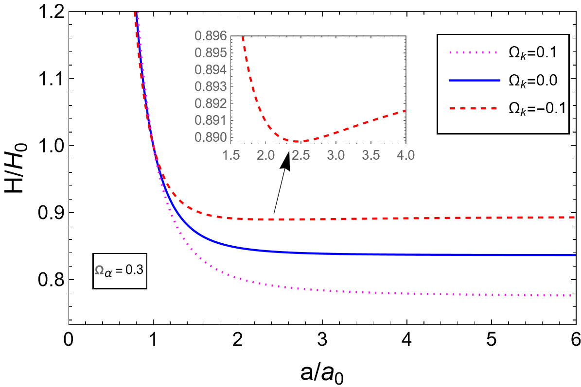
Figure 1: The evolution of the Hubble parameter $H$ with respect to the cosmic scale factor $a$ for a fixed value of $\Omega_{\alpha}~{}(=0.3)$ has been depicted for three spatial geometries of the universe, namely, open universe, flat universe, and closed universe.

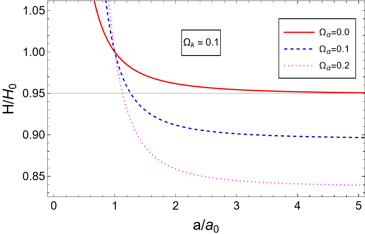
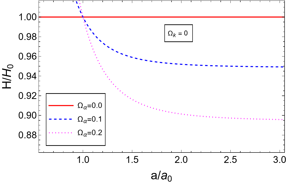
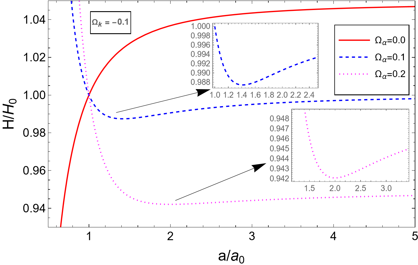
Figure 2: We display the evolution of the Hubble function for different values of $\Omega_{\alpha}$ considering three spatial geometries of the universe, namely, open universe (upper left graph), flat universe (upper right graph) and closed universe (lower graph).

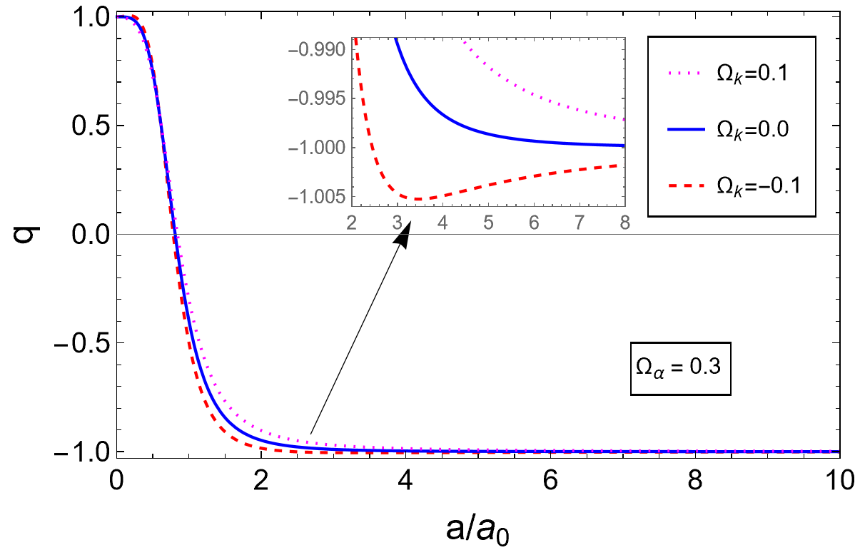
Figure 3: The evolution of the deceleration parameter for a fixed value of $\Omega_{\alpha}~{}(=0.3)$ has been shown for different spatial geometries of the universe, namely, open universe, flat universe, and closed universe.

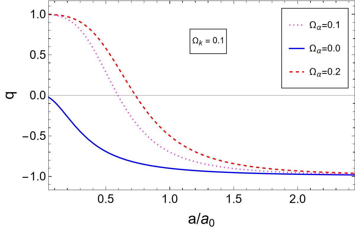
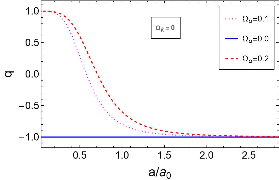
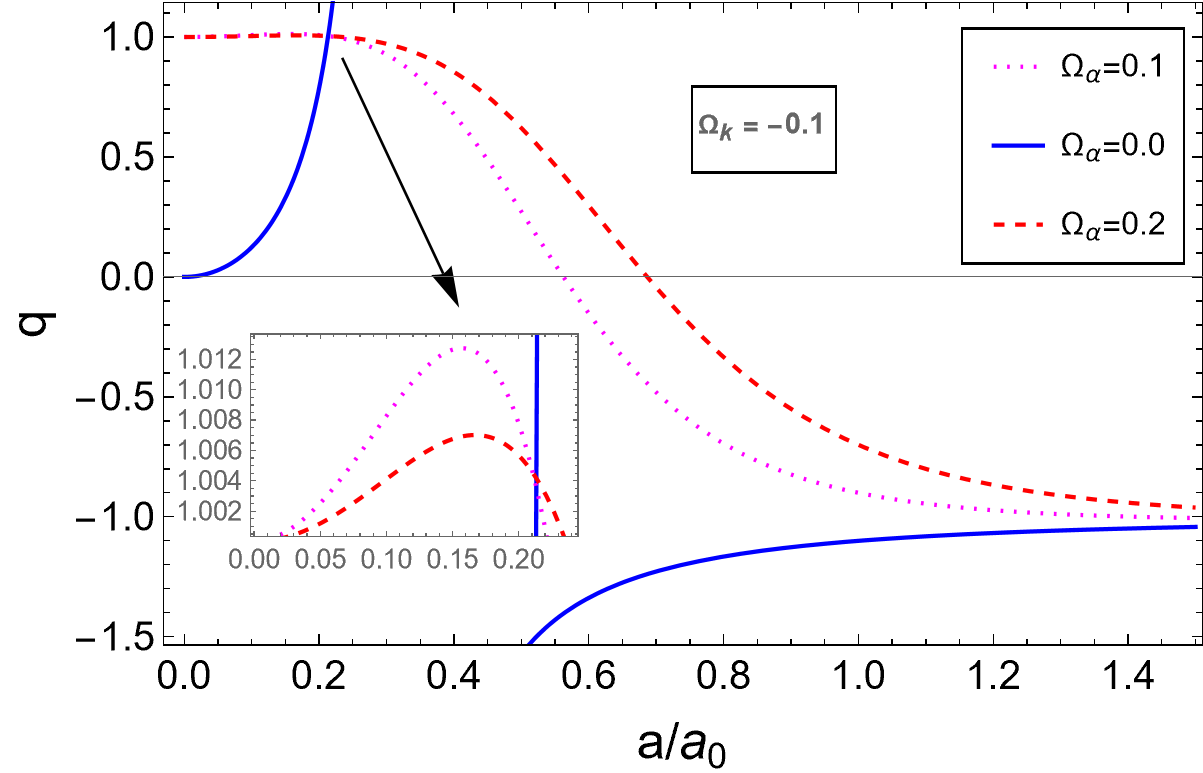
Figure 4: We present the evolution of the deceleration parameter for different $\Omega_{\alpha}$ considering three spatial geometries of the universe, namely, open universe (upper left graph), flat universe (upper right graph) and closed universe (lower graph).

V Results and their Implications

Let us finally discuss the major consequences the novel Time Crystal-like condensate can have on the evolution of the universe. As described in section IV, the TC background can provide an expression for the scale factor $a(t)$ in terms of density parameters $\Omega_{j}$ ($j=\Lambda,\alpha,k$). This leads to two of the well-known cosmological parameters, namely, the Hubble parameter $H(a)$ and the deceleration parameter $q(a)$ which offer a clear picture of the dynamics of our universe. In order to understand the dynamics of the universe, in Figs. 1, 2, 3, 4, we provide the graphical descriptions of $H(a)$ and $q(a)$ in various curvature scenarios and strengths of the TC condensate through $\alpha$ (generated by the $\alpha R^{2}$-term in gravity). In all the figures, $\Omega_{k}$ can take positive, negative or zero value corresponding to open (negative curvature), closed (positive curvature) or flat (zero curvature) universe, respectively.

In Fig. 1, for a fixed value of $\Omega_{\alpha}=0.3$, the evolution of the dimensionless Hubble parameter $H/H_{0}$ is displayed against $a/a_{0}$ for positive, negative and vanishing $\Omega_{k}$. Since from eqn. (41), it is clear that $\Omega_{\Lambda},\Omega_{\alpha}$ are always positive but $\Omega_{k}$ can change sign as $k$ can take three distinct values ($0,+1,-1$), and only for the negative $\Omega_{k}$ (i.e. positive curvature or closed universe), it contributes oppositely and there is the possibility of a stationary point (in the present case a minimum) in $H(a)~{}vs.~{}a$ profile.

To establish the effects of TC condensate clearly, in Fig. 2, we plot the evolution of the Hubble parameter in terms of $a/a_{0}$ for three distinct spatial geometries of the universe, namely, $\Omega_{k}=+0.1$ (upper left graph of Fig. 2), $\Omega_{k}=0$ (upper right graph of Fig. 2) and $\Omega_{k}=-0.1$ (lower graph of Fig. 2), respectively, and for each case we take three distinct values of $\Omega_{\alpha}$ as $\Omega_{\alpha}=0,0.1,0.2$ keeping in mind that it is positive and small and fixing $\Omega_{\Lambda}$ accordingly. Notice that for $\Omega_{k}>0$ (open universe) the profiles are qualitatively similar (see the upper left graph of Fig. 2) with only quantitative differences as $\Omega_{\alpha}$ increases. However, the graphs change significantly for $\Omega_{k}=0$ (flat universe) where $\Omega_{\alpha}=0$ yields the well-known constant value of $H(a)$ but non-zero $\Omega_{\alpha}$’s show distinct variation of $H(a)$ with respect to $a$ (see the upper right graph of Fig. 2). Once again, the $\Omega_{k}<0$, see the lower graph of Fig. 2 (closed universe) is the most interesting scenario where non-zero values of $\Omega_{\alpha}$ generate completely different profiles compared to $\Omega_{\alpha}=0$ (no TC condensate); the former ones have a minimum before saturating for large $a$. It is also easy to see from eqn. (39) that all the curves for different $\Omega_{\alpha}$ will cross at $a=a_{0}$.

Now we study the behavior of the deceleration parameter $q(a)$ for the same sets of parameters as considered earlier. Fig. 3 demonstrates a very interesting fact that for any universe (with $\Omega_{k}$ being positive, negative or zero), a non-trivial $\Omega_{\alpha}$ induces a change in the sign of $q(a)$ from positive to negative as $a$ increases from 0. This indicates that the TC condensate generates a decelerating phase before the acceleration starts. Clearly this indicates that after initial contracting phase (deceleration) the universe changes to an expanding phase (acceleration).

Once again we analyse the strength of $\Omega_{\alpha}$ for the three different spatial structures of the universe. In Fig. 4 we have summarized the evolution of the deceleration parameter for $\Omega_{k}$ being positive (corresponds to the upper left graph of Fig. 4), zero (upper right graph of Fig. 4) and negative (lower graph of Fig. 4) respectively, taking three distinct values of $\Omega_{\alpha}$ characterizing the strength of the TC background, namely, $\Omega_{\alpha}=0,0.1,0.2$. The upper left graph of Fig. 4 (corresponds to $\Omega_{k}>0$) and the upper right graph of Fig. 4 ($\Omega_{k}=0$) show the emergence of the decelerating phase in the early universe before the accelerating phase ensues for all three values of $\Omega_{\alpha}$. However, from the lower graph of Fig. 4 (corresponds to $\Omega_{k}<0$), we find that the condensate can ameliorate the singularity in $q(a)$ in the conventional case without the $\alpha R^{2}$ term. This is clear from eqn. (45) where with $\Omega_{\alpha}=0$, $q$ will become singular at $a/a_{0}={\sqrt{\Omega_{k}/\Omega_{\Lambda}}}$ for negative $\Omega_{k}$.

Let us recall that in conventional cosmology, a decelerating phase can appear only if matter is introduced from outside. However, in our case, no external matter is introduced and this contracting phase is generated solely by the TC condensate (coming from the $\alpha R^{2}$ term). We speculate that the TC condensate might be identified as a new kind of matter candidate having radiation-like behaviour. The upper left and right plots of Fig. 4 show how the strength of the TC condensate affects the behavior of $q$ through different curves that merge with the $\Omega_{\alpha}=0$ curve asymptotically. However, the situation is very different for $\Omega_{k}=-0.1$ as depicted in the lower graph of Fig. 4 . In small $a$ sector, there appears a discontinuity in $q$ for $\Omega_{\alpha}=0$ (standard GR, no $R^{2}$-term hence no condensate) that is smoothed out for non-zero $\Omega_{\alpha}$ ($R^{2}$-term with condensate effect) and finally all curves asymptotically saturate to a negative $q$ at large $a$.

VI Summary and Conclusions

The idea of TC was a fascinating concept in physics and due to its attractive physical insights, this created a significant amount of interest in the physics community within a couple of years of its theoretical possibility Wilczek (2012) (also see Shapere and Wilczek (2012); Ghosh (2014); Sacha and Zakrzewski (2018). As argued by several investigators TC could have some effects on cosmological dynamics Bains et al. (2017); Vacaru (2018); Addazi et al. (2019); Feng et al. (2020); Das et al. (2019); Yoshida and Soda (2019); Li et al. (2019); Li and Piao (2020); Bubuianu et al. (2021) and this should be further explored. However, an important qualitative distinction between TC as introduced in cosmology and TCC, induced by quadratic $R^{2}$ term, as considered here, needs to be emphasized. Whereas in previous works, the TC crystal feature was incorporated in the externally introduced matter sector, however, in the present case, the TCC is generated internally from the combinations of the metric tensor components iff $R^{2}$-term in the gravity action exists.

Following this, in the present article we have investigated the effects of TCC in cosmology aiming to understand whether the TCC could offer some interesting features about the intrinsic nature of our mysterious universe. According to the past historical records, physics at the early and late evolution of our universe has put several question marks on the understanding of our universe and its origin as well. The fundamental questions related to the universe evolution are still need to be answered.

As has been mentioned throughout, we exploit the property of $f(R)\sim R+\alpha R^{2}$ that it gives rise to a decoupled system of conventional gravity and a higher derivative scalar sector and propose a model where the former evolves in a background of the latter, which enjoys a TC phase. Thus, the energy-momentum tensor for the corresponding TCC acts as a source for cosmological dynamics, characterized by the FLRW line element. We found that the scale factor of the FLRW universe can be analytically solved under some approximations and hence the other cosmological parameters. The behaviour of the cosmological parameters, namely, the Hubble rate ($H(a)$) and the deceleration parameter ($q(a)$) have been graphically presented (see Figs. 1, 2, 3, 4) for different spatial geometries of the universe and for different strengths of the TC condensate through $\alpha$ generated by the $\alpha R^{2}$-term in the gravitational action. We found some interesting observations that clearly report that the TC condensate can significantly affect the cosmological dynamics. From the evolution of the Hubble rate for a closed universe (see the lower graph of Fig. 2) we notice that the non-zero values of $\Omega_{\alpha}$ generate completely different profiles compared to $\Omega_{\alpha}=0$ (no TC condensate) the former ones have a minimum before saturating for large $a$. On the other hand, from Fig. 3, we notice that irrespective of the spatial geometry of the universe, the TC condensate generates a decelerating phase before the acceleration starts. This indicates that after initial contracting phase (deceleration) of the universe, it enters into an expanding phase with an acceleration. As the non-trivial $\Omega_{\alpha}$ offers some interesting results independent of the curvature of the universe, therefore, in Fig. 4 we further investigated how the evolution of the deceleration parameter depends on various strengths of the TC condensate quantified through $\Omega_{\alpha}$ for different spatial geometries. For $\Omega_{k}>0$ (upper left plot of Fig. 4), $\Omega_{k}=0$ (upper right plot of Fig. 4) universe enters into the early accelerating phase before a decelerating phase and this remains true for different three values of $\Omega_{\alpha}$. However, for the closed universe (corresponds to the lower graph of Fig. 4), we find that the TC condensate can avoid the singularity in $q(a)$ that appears in the conventional case without the $\alpha R^{2}$ term.

The final take home message of our analysis is the following: the generic ghost problem in higher order gravity theories is absent in $R^{2}$-gravity which, however, is still plagued with the (relatively harmless) additional (spurious) scalar degree of freedom. We have shown that in the Time Crystal framework, this extra scalar can act as a condensate, that replaces the vacuum, forms a stable background for conventional gravity, leading to possible improvements with explicit predictions.

Following the existing results and the present outcomes in context of late and early universe, we anticipate that the physics of TC condensate needs considerable attention in the cosmological dynamics. In particular, the existence of some radiation-like fluid extracted (purely) out of the geometrical sector strongly highlights this fact. One may naturally wonder whether TC condensate may lead to some geometrical dark energy in the early universe (early dark energy fluid) Poulin et al. (2019) that could offer some new insights in the cosmological tensions Di Valentino et al. (2021); Kamionkowski and Riess (2022). One can further investigate whether the finite time future singularities appearing in the cosmological theories can be avoided in this context Caldwell et al. (2003); Nojiri et al. (2005). There is no doubt that being an emerging field, understanding the nature and the effects of TC condensate, could open new windows in cosmology and astrophysics. It will be interesting to explore further the effects of TC condensate in alternative gravitational theories other than the quadratic $f(R)$ gravity. We hope to investigate some of them in near future.

VII Acknowledgments

RKD acknowledges Naresh Saha and Joydeep Majhi for helpful discussions. SP acknowledges the financial support from the Department of Science and Technology (DST), Govt. of India under the Scheme “Fund for Improvement of S&T Infrastructure (FIST)” (File No. SR/FST/MS-I/2019/41).

References

- Alvarez-Gaume et al. (2016) L. Alvarez-Gaume, A. Kehagias, C. Kounnas, D. Lüst, and A. Riotto, Fortsch. Phys. 64, 176 (2016), arXiv:1505.07657 [hep-th] .
- Chakraborty and Ghosh (2022) S. Chakraborty and S. Ghosh, Phys. Dark Univ. 35, 100976 (2022), arXiv:2001.04680 [gr-qc] .
- Wilczek (2012) F. Wilczek, Phys. Rev. Lett. 109, 160401 (2012), arXiv:1202.2539 [quant-ph] .
- Shapere and Wilczek (2012) A. Shapere and F. Wilczek, Phys. Rev. Lett. 109, 160402 (2012), arXiv:1202.2537 [cond-mat.other] .
- Ghosh (2014) S. Ghosh, Physica A: Statistical Mechanics and its Applications 407, 245 (2014), arXiv:1208.4438 [hep-th] .
- Sacha and Zakrzewski (2018) K. Sacha and J. Zakrzewski, Rept. Prog. Phys. 81, 016401 (2018), arXiv:1704.03735 [quant-ph] .
- Das et al. (2018) P. Das, S. Pan, S. Ghosh, and P. Pal, Phys. Rev. D 98, 024004 (2018), arXiv:1801.07970 [hep-th] .
- Bains et al. (2017) J. S. Bains, M. P. Hertzberg, and F. Wilczek, JCAP 05, 011 (2017), arXiv:1512.02304 [hep-th] .
- Vacaru (2018) S. I. Vacaru, Class. Quant. Grav. 35, 245009 (2018), arXiv:1803.04810 [physics.gen-ph] .
- Addazi et al. (2019) A. Addazi, A. Marcianò, R. Pasechnik, and G. Prokhorov, Eur. Phys. J. C 79, 251 (2019), arXiv:1804.09826 [hep-th] .
- Feng et al. (2020) X.-H. Feng, H. Huang, S.-L. Li, H. Lü, and H. Wei, Eur. Phys. J. C 80, 1079 (2020), arXiv:1807.01720 [hep-th] .
- Das et al. (2019) P. Das, S. Pan, and S. Ghosh, Phys. Lett. B 791, 66 (2019), arXiv:1810.06606 [hep-th] .
- Yoshida and Soda (2019) D. Yoshida and J. Soda, Phys. Rev. D 100, 123531 (2019), arXiv:1909.05533 [hep-th] .
- Li et al. (2019) S.-L. Li, H. Lü, H. Wei, P. Wu, and H. Yu, Phys. Rev. D 99, 104057 (2019), arXiv:1903.03940 [gr-qc] .
- Li and Piao (2020) H.-H. Li and Y.-S. Piao, Phys. Lett. B 801, 135156 (2020), arXiv:1907.09148 [gr-qc] .
- Bubuianu et al. (2021) I. Bubuianu, S. I. Vacaru, and E. V. Veliev, Eur. Phys. J. Plus 136, 149 (2021), arXiv:1907.05847 [physics.gen-ph] .
- Nojiri and Odintsov (2006) S. Nojiri and S. D. Odintsov, eConf C0602061, 06 (2006), arXiv:hep-th/0601213 .
- Nojiri et al. (2017) S. Nojiri, S. D. Odintsov, and V. K. Oikonomou, Phys. Rept. 692, 1 (2017), arXiv:1705.11098 [gr-qc] .
- Capozziello and Francaviglia (2008) S. Capozziello and M. Francaviglia, Gen. Rel. Grav. 40, 357 (2008), arXiv:0706.1146 [astro-ph] .
- Padmanabhan (2008) T. Padmanabhan, Gen. Rel. Grav. 40, 529 (2008), arXiv:0705.2533 [gr-qc] .
- Sotiriou and Faraoni (2010) T. P. Sotiriou and V. Faraoni, Rev. Mod. Phys. 82, 451 (2010), arXiv:0805.1726 [gr-qc] .
- Silvestri and Trodden (2009) A. Silvestri and M. Trodden, Rept. Prog. Phys. 72, 096901 (2009), arXiv:0904.0024 [astro-ph.CO] .
- De Felice and Tsujikawa (2010) A. De Felice and S. Tsujikawa, Living Rev. Rel. 13, 3 (2010), arXiv:1002.4928 [gr-qc] .
- Nojiri and Odintsov (2011) S. Nojiri and S. D. Odintsov, Phys. Rept. 505, 59 (2011), arXiv:1011.0544 [gr-qc] .
- Clifton et al. (2012) T. Clifton, P. G. Ferreira, A. Padilla, and C. Skordis, Phys. Rept. 513, 1 (2012), arXiv:1106.2476 [astro-ph.CO] .
- Hinterbichler (2012) K. Hinterbichler, Rev. Mod. Phys. 84, 671 (2012), arXiv:1105.3735 [hep-th] .
- Capozziello and De Laurentis (2011) S. Capozziello and M. De Laurentis, Phys. Rept. 509, 167 (2011), arXiv:1108.6266 [gr-qc] .
- Sami and Myrzakulov (2016) M. Sami and R. Myrzakulov, Int. J. Mod. Phys. D 25, 1630031 (2016), arXiv:1309.4188 [hep-th] .
- de Rham (2014) C. de Rham, Living Rev. Rel. 17, 7 (2014), arXiv:1401.4173 [hep-th] .
- Cai et al. (2016) Y.-F. Cai, S. Capozziello, M. De Laurentis, and E. N. Saridakis, Rept. Prog. Phys. 79, 106901 (2016), arXiv:1511.07586 [gr-qc] .
- Bahamonde et al. (2023) S. Bahamonde, K. F. Dialektopoulos, C. Escamilla-Rivera, G. Farrugia, V. Gakis, M. Hendry, M. Hohmann, J. Levi Said, J. Mifsud, and E. Di Valentino, Rept. Prog. Phys. 86, 026901 (2023), arXiv:2106.13793 [gr-qc] .
- Gibbons et al. (2019) G. W. Gibbons, C. N. Pope, and S. Solodukhin, Phys. Rev. D 100, 105008 (2019), arXiv:1907.03791 [hep-th] .
- Poulin et al. (2019) V. Poulin, T. L. Smith, T. Karwal, and M. Kamionkowski, Phys. Rev. Lett. 122, 221301 (2019), arXiv:1811.04083 [astro-ph.CO] .
- Di Valentino et al. (2021) E. Di Valentino, O. Mena, S. Pan, L. Visinelli, W. Yang, A. Melchiorri, D. F. Mota, A. G. Riess, and J. Silk, Class. Quant. Grav. 38, 153001 (2021), arXiv:2103.01183 [astro-ph.CO] .
- Kamionkowski and Riess (2022) M. Kamionkowski and A. G. Riess, (2022), arXiv:2211.04492 [astro-ph.CO] .
- Caldwell et al. (2003) R. R. Caldwell, M. Kamionkowski, and N. N. Weinberg, Phys. Rev. Lett. 91, 071301 (2003), arXiv:astro-ph/0302506 .
- Nojiri et al. (2005) S. Nojiri, S. D. Odintsov, and S. Tsujikawa, Phys. Rev. D 71, 063004 (2005), arXiv:hep-th/0501025 .