A PROLETARIAN APPROACH TO GENERATING

EIGENVALUES OF GUE MATRICES

Luc Devroye^∗ and Jad Hamdan^†

^∗School of Computer Science, McGill University,

^†Mathematical Institute, University of Oxford

Abstract. We propose a simple algorithm to generate random variables described by densities equaling squared Hermite functions. Using results from random matrix theory, we utilize this to generate a randomly chosen eigenvalue of a matrix from the Gaussian Unitary Ensemble (gue) in sublinear expected time in the ram model. Keywords. Random variate generation, orthogonal polynomials, Hermite functions, rejection method, random matrices, Gaussian unitary ensemble, eigenvalues.

.  ntroduction

In this note, we concern ourselves with the generation of a random eigenvalue of a matrix in the Gaussian Unitary Ensemble gue$(n)$, described by the Gaussian measure with density

$$(2^{n/2}\pi^{n^{2}/2})^{-1}e^{-(n/2)\,\text{tr}H^{2}}$$

on the space of $n\times n$ Hermitian matrices $H=(H_{ij})_{i,j=1}^{n}$.

We operate under the ram model, meaning that we assume that real numbers can be stored and operated upon in one time unit. Besides the standard operators, we also assume constant time performance for the exponential, logarithmic, trigonometric and gamma functions. We also assume that a source capable of producing an i.i.d. sequence of uniform $[0,1]$ random variables is available.

The problem of computing the eigenvalues of an arbitrary (deterministic) matrix is as old as it is well–studied. It follows from the Abel–Ruffini theorem (see [1], [15]) that no exact finite–time algorithm exists that finds roots of polynomials of degree greater than 5. One therefore typically resorts to approximation algorithms to find eigenvalues of matrices of higher dimension. Most are quite efficient, including the Lanczos algorithm [10] and the Rayleigh quotient iteration [9] for Hermitian matrices, or, more generally, the power iteration [21]. One therefore obtains an approximate method for generating eigenvalues of a random gue$(n)$ matrix by first constructing a matrix from this ensemble (which can be done entry-wise, as outlined in [3]), and then approximating its eigenvalues. At the very best these methods take quadratic time in $n$.

However, our primary concern is that of both efficiency and exactness. For $n\leq 4$, one can simply construct a gue$(n)$ matrix and directly compute the roots of its characteristic polynomial. We are not bothered by the fact that this runs in factorial time given how small $n$ is, but are left needing an approach that generalizes to $n\geq 5$.

We begin by proposing, in section 2, an algorithm to sample a random uniformly selected gue$(n)$ eigenvalue whose expected runtime is sublinear in $n$. It relies on the fact that our problem can be reduced to that of generating random variables described by densities equal to squared Hermite functions, defined below. We then sample from these distributions using the rejection method [22].

It is known (see [3]) that the joint distribution of the eigenvalues $\lambda_{1}(M),...,\lambda_{n}(M)$ of a gue$(n)$ matrix $M$ has Lebesgue density

$$C_{n}\mathbf{1}_{[x_{1}\leq...\leq x_{n}]}\prod_{i<j}^{n}(x_{j}-x_{i})^{2}\prod_{i=1}^{n}e^{-x_{i}^{2}/2},$$ (1)

where $C_{n}$ is a normalization constant. Using the rejection method applied to a dominating density for (1), we then propose a much slower algorithm that instead generates the entire vector of $n$ eigenvalues of a gue$(n)$ matrix. This is explained in section 3.

1.1.  The density of a random gue eigenvalue

For a distribution on sets of $n$ points, the $k-$point correlation function $\sigma_{k}(x_{1},...,x_{k})$ describes the induced probability distribution on uniformly selected subsets of size $k\leq n$. It is typically normalized so that $\frac{1}{n}\sigma_{n}(x)$ is the probability density function of a uniformly selected (set of $1$) point. It is well-known (see [7]) that for gue$(n)$ eigenvalues, the $k-$point correlation function is given by a $k\times k$ determinant $\det(K(x_{1},x_{2}))_{1\leq i,j\leq k}$, where

$$K(x,y)=\frac{1}{\sqrt{2\pi}}\sum_{k=0}^{n-1}\frac{H_{k}(x)H_{k}(y)e^{-(x+y)^{2}/4}}{k!}=\sum_{k=0}^{n-1}\phi_{k}(x)\phi_{k}(y).$$

In the expression above, $H_{k}$ is the $k$-th Hermite polynomial

$$H_{k}(x)=(-1)^{k}e^{x^{2}/2}\bigg{(}\frac{d}{dx}\bigg{)}^{k}e^{-x^{2}/2},$$

and $\phi_{k}$ is the so-called Hermite function $H_{k}(x)e^{-x^{2}/4}/\sqrt{k!\sqrt{2\pi}}$ (in the theory of orthogonal functions, $K(x,y)$ is known as the Christoffel-Darboux kernel [18]). The probability density for the distribution of a single, uniformly selected eigenvalue from a gue$(n)$ matrix is thus equal to

$$\frac{1}{n}K(x,x)=\frac{1}{n}\sum_{k=0}^{n-1}\phi_{k}(x)^{2}.$$ (2)

We remark in passing that, using asymptotic properties of Hermite polynomials (see [13]), one can recover Wigner’s famous semi-circle law [23] from this expression.

Next, we note that Hermite polynomials are orthogonal. In particular, for any $k\in\mathbf{N}$, we have

$$\int_{-\infty}^{\infty}H_{k}(x)^{2}e^{-x^{2}/2}dx=\sqrt{2\pi}\,k!$$

(see [16] for a proof), which shows that $\phi_{k}^{2}$ is a density for every $k$. It then follows from (2) that if one picks an index $k\in\{0,\dots,n-1\}$ uniformly at random and generates a random variate described by the density $\phi_{k}^{2}$, the result would be distributed as a uniformly selected gue$(n)$ eigenvalue. The remainder of this paper (with the exception of section 3) will focus on generating random variables described by the densities $\phi_{k}^{2}$.

.  enerating from Densities equal to squared Hermite functions

2.1.  Notation and preliminaries on Hermite polynomials

The aforementioned Hermite polynomials can alternatively be defined using the recurrence $H_{0}=1$, $H_{1}(x)=x$ and

$$H_{k+1}(x)=xH_{k}(x)-kH_{k-1}(x)$$ (3)

for any $k\geq 2$, giving us a simple $O(k)$ algorithm to compute $H_{k}$ for fixed $x$ ([18]). We also have the following theorem, due to Bonan & Clarke [4], which gives an upper bound for $\phi_{n}^{2}$ on $\mathbf{R}$. Note that we computed the explicit constants).

Theorem 1.

For any $n\in\mathbf{N}$, let $\phi_{n}^{2}$ be the square of the $n-$th Hermite function (defined in the previous section). Then

$$\sup_{x\in\mathbf{R}}\phi_{n}^{2}(x)\leq\frac{8(\pi+1)}{3}\cdot n^{-1/6}.$$

Furthermore,

$$\phi_{n}^{2}(x)\leq\begin{cases}\frac{8\pi}{3}(\sqrt{4n+2-x^{2}})^{-1},&\text{if $|x|\leq\sqrt{4n+2}$,}\\ {2\sqrt{2}B^{2}n^{-5/6}}(\sqrt{4n+2}-x)^{-4},&\text{if $|x|>\sqrt{4n+2}$}.\end{cases}$$

where $B=(\pi+1)^{2}\sqrt{8(\pi+1)/3}$.

If we let

$$x_{1}=x_{1}(n)=\sqrt{4n+2-\frac{\pi^{2}}{(\pi+1)^{2}}\,n^{1/3}}$$

and

$$x_{2}=x_{2}(n)=\sqrt{4n+2}+\sqrt{B}\bigg{(}\frac{3}{2\sqrt{2}(\pi+1)}\bigg{)}^{1/4}n^{-1/6},$$

it follows directly from the theorem above that the function

$$h_{n}(x)\stackrel{{\scriptstyle\text{def}}}{{=}}\begin{cases}\frac{8\pi}{3}(\sqrt{4n+2-x^{2}})^{-1},&\text{if $|x|\leq x_{1}$,}\\ \frac{8(\pi+1)}{3}\cdot n^{-1/6},&\text{if $|x|\in(x_{1},x_{2}]$,}\\ {2\sqrt{2}B^{2}n^{-5/6}}(\sqrt{4n+2}-x)^{-4},&\text{if $|x|>x_{2}$,}\end{cases}$$

dominates $\phi_{n}^{2}$ on all of $\mathbf{R}$.

The following lemma will be useful in the analysis of our algorithm’s expected runtime.

Lemma 2.

Let $h_{n}$ be defined as above. Then

$$\int_{\mathbf{R}}h_{n}(x)\,dx=O(1),\quad\int_{x_{1}}^{\infty}h_{n}(x)\,dx=O(n^{-1/3}).$$

Proof.

Let $n\in\mathbf{N}$ be arbitrary, then

$$\int_{\mathbf{R}}h_{n} =\int_{0}^{x_{1}}\frac{8\pi}{3}\frac{1}{\sqrt{4n+2-x^{2}}}dx+\int_{x_{1}}^{x_{2}}\frac{8(\pi+1)}{3}\cdot n^{-1/6}dx+\int_{x_{2}}^{\infty}\frac{2\sqrt{2}B^{2}n^{-5/6}}{(\sqrt{4n+2}-x)^{4}}dx$$

$$=\frac{8\pi}{3}\arcsin{\frac{x_{1}}{\sqrt{4n+2}}}+\frac{8(\pi+1)n^{-1/6}}{3}|x_{2}-x_{1}|+\frac{\sqrt{B}\,2\sqrt{2}}{3}\bigg{(}\frac{2\sqrt{2}(\pi+1)}{3}\bigg{)}^{3/4}n^{-1/3}$$

and the lemma follows from the fact that $|x_{2}-x_{1}|=O(n^{-1/6})$. ∎

We will also need the following representation of Hermite polynomials due to van Veen [20].

Theorem 3.

For any $n,k\in\mathbf{N}$, $x\in[0,2\sqrt{n+1}]$,

$$H_{n}(x) =A_{n}(x)\big{(}B_{n}(x)+\mu R_{n}(x)\big{)}$$

where

$$A_{n}(x)\overset{\text{def}}{=}\frac{\Gamma(n+1)}{\pi}\frac{e^{{(n+1)}/2+x^{2}/4}}{(n+1)^{n/2}},$$

$$B_{n}(x)\stackrel{{\scriptstyle\text{def}}}{{=}}\frac{\sqrt{\pi}}{\left\{(n+1)\sin(\alpha)\right\}^{1/2}}*\sin\left\{\frac{(n+1)}{2}\big{(}\sin(2\alpha)-2\alpha\big{)}+\frac{\alpha}{2}+\frac{3\pi}{4}\Big{)}\right\},$$

$$R_{n}(x)\overset{\text{def}}{=}\frac{1}{3(n+1)\sin(\alpha)^{2}},$$

$\mu$ is a constant whose absolute value is no greater than $4.2$ and

$$\alpha=\alpha(x)=\arccos{\frac{x}{2\sqrt{n+1}}}.$$

This representation is then extended to $|x|\leq 2\sqrt{n+1}$ using the fact that $H_{n}$ is even. On said domain, for any $n,k\in\mathbf{N}$, we use $V_{n}\stackrel{{\scriptstyle\text{def}}}{{=}}A_{n}*B_{n}$ (as defined in the theorem above) to approximate $H_{n}$ and define the following approximation to $\phi_{n}^{2}$:

$$f_{n}(x)\stackrel{{\scriptstyle\text{def}}}{{=}}\frac{V_{n}(x)^{2}e^{-x^{2}/2}}{{\sqrt{2\pi}\,n!}}$$

(we define $f_{n}=0$ if $|x|>2\sqrt{n+1}$). Note that for any $|x|<2\sqrt{n+1}$,

$$|\phi_{n}^{2}(x)-f_{n}(x)|=\bigg{(}\big{(}\mu R_{n}(x)\big{)}^{2}+2\mu R_{n}(x)B_{n}(x)\bigg{)}\frac{A_{n}^{2}(x)e^{-x^{2}/2}}{\sqrt{2\pi}\,n!}.$$

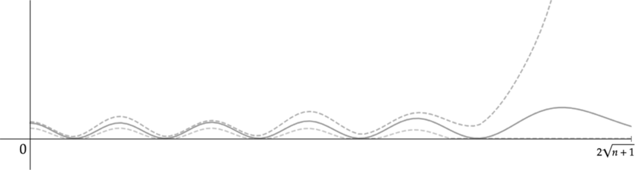
Figure 1: The function $\phi_{10}^{2}$ (bold) bounded from below and above by $(f_{10}-\epsilon^{-})_{+}$ and $(f_{10}+\epsilon^{+})$ (dotted).

Using the fact that $|\mu|<4.2$, it follows that

$$(\phi_{n}^{2}(x)-f_{n}(x))_{+}\,\leq\, \epsilon^{+}(x)\stackrel{{\scriptstyle\text{def}}}{{=}}\frac{A_{n}^{2}(x)e^{-x^{2}/2}}{\sqrt{2\pi}\,n!}\big{(}(8.4)(B_{n}(x))_{+}R_{n}(x)+(4.2)^{2}R_{n}(x)^{2}\big{)}$$

$$(\phi_{n}^{2}(x)-f_{n}(x))_{-}\,\leq\, \epsilon^{-}(x)\stackrel{{\scriptstyle\text{def}}}{{=}}\frac{A_{n}^{2}(x)e^{-x^{2}/2}}{\sqrt{2\pi}\,n!}(8.4)\bigg{(}\Big{(}B_{n}(x)R_{n}(x)\Big{)}_{+}\lor\Big{(}B_{n}(x)R_{n}(x)\Big{)}_{-}\bigg{)}$$

(we used $a\wedge b$ (resp. $a\lor b$) to denote $\min(a,b)$ (resp. $\max(a,b)$) and $(x)_{+}=(x\lor 0)$, $(x)_{-}=(-x\lor 0)$). Note that $\epsilon^{+/-}$ are positive by definition and

$$\left(f_{n}-\epsilon^{-}\right)_{+}\leq\phi_{n}^{2}\leq\left(f_{n}+\epsilon^{+}\right)\wedge h_{n}$$ (4)

for any $x\in\mathbf{R}$. Lastly, we define $\Delta_{\epsilon}(x)$ to be the gap between the upper and lower bound for $\phi_{n}^{2}(x)$ and note that there exists a constant $C$ for which

$$\Delta_{\epsilon}(x) \leq C\bigg{(}\big{|}R_{n}(x)|^{2}+|R_{n}(x)B_{n}(x)|\bigg{)}\frac{A_{n}^{2}(x)e^{-x^{2}/2}}{\sqrt{2\pi}\,n!}$$

and the following proposition holds.

Proposition 4.

For large enough $n$,

$$\int_{0}^{x_{1}}\Delta_{\epsilon}(x)\,dx=O\big{(}n^{-1/3}\big{)}.$$

Proof.

See appendix. ∎

2.2.  Generating random variates described by $h_{n}/\int h_{n}$

Our main algorithm in the following section requires the generation of random variates described by the density $h_{n}/\int h_{n}$. This can be done in constant expected time using the following algorithm, which is a straightforward application of the inversion method (see [5] for a thorough exposition of this method).

⬇

ALGORITHM 1:

Generate $S$, where $\mathbf{P}\{S=1\}=\mathbf{P}\{S=-1\}=1/2$.

Generate $U$ uniformly on $[0,1]$.

IF $U<p_{1}/(p_{1}+p_{2}+p_{3})$ THEN

Generate $V$ uniformly on $[0,1]$.

$X\leftarrow\sqrt{4n+2}\,\,\big{|}\sin(V*\arcsin(x_{1}/\sqrt{4n+1}))\big{|}$

ELSE IF $p_{1}/(p_{1}+p_{2}+p_{3})\leq U<(p_{1}+p_{2})/(p_{1}+p_{2}+p_{3})$ THEN

Generate $V$ uniformly on $[0,1]$.

$X\leftarrow x_{1}+(x_{2}-x_{1})*V$

ELSE

Generate $V$ uniformly on $[0,1]$.

$X\leftarrow\sqrt{4n+2}\,+\,{\sqrt{B}\bigg{(}\frac{3}{2\sqrt{2}(\pi+1)}\bigg{)}^{1/4}n^{-1/6}}*{V^{-1/3}}$

RETURN $X*S$

where

$$p_{1} =\int_{0}^{x_{1}}h_{n}=\frac{8\pi}{3}\arcsin{\frac{x_{1}}{\sqrt{4n+2}}},$$

$$p_{2} =\int_{x_{1}}^{x_{2}}h_{n}=\frac{8(\pi+1)}{3}n^{-1/6}\big{|}x_{2}-x_{1}\big{|},$$

$$p_{3} =\int_{x_{2}}^{\infty}h_{n}=\sqrt{B}\cdot\left(\frac{2\sqrt{2}}{3}\right)^{7/4}(\pi+1)^{3/4}n^{-1/3}.$$

2.3.  A first eigenvalue algorithm that is linear in $n$

For any $n$, we now know how to generate from $h_{n}/\int h_{n}$ and that $h_{n}$ dominates $\phi_{n}^{2}$. The following rejection algorithm (see [5] and [22]) will be used as a stepping stone towards our main algorithm, and will be shown to run in linear time in the following section.

⬇

ALGORITHM 2:

REPEAT UNTIL ACCEPT

Generate $X$ from $h_{n}/\int h_{n}$

Generate $U$ uniformly on $[0,1]$

ACCEPT $\leftarrow\big{[}U*h_{n}(X)\leq\phi_{n}^{2}(X)\big{]}$

RETURN $X$

Note that the comparison requires us to compute $\phi_{n}^{2}(X)$, which we do using the recurrence relation for Hermite polynomials (3) given earlier.

2.4.  Main algorithm and runtime analysis

We can refine this second algorithm using van Veen’s estimate for $H_{n}$ stated in Theorem 3. Let $\phi_{n}^{2}$, $f_{n}$, $h_{n}$, and $\epsilon^{+/-}$ be defined as above.

⬇

ALGORITHM 3:

REPEAT FOREVER

Generate $X$ from $h_{n}/\int h_{n}$

Generate $U$ uniformly on $[0,1]$

IF $U*h_{n}(X)\leq\left(f_{n}(X)-\epsilon^{-}(X)\right)_{+}$ RETURN X

ELSE IF $U*h_{n}(X)\leq\left(f_{n}(X)+\epsilon^{+}(X)\right)$ THEN

IF $U*h_{n}(X)\leq\phi^{2}_{n}(X)$ RETURN X

We emphasize that $f_{n},h_{n}$ and $\epsilon^{+/-}$ can be computed in $O(1)$ time, and note that in the last line, $\phi_{n}^{2}$ is computed using the recurrence formula given above, as in algorithm 2.

Fix $n\in\mathbf{N}$, and let $N$ be the number of iterations of algorithm 3 when generating from $\phi_{n}^{2}$. Let $T_{i}$ be the time taken by the $i$-th iteration, where $1\leq i\leq N$, then the total runtime of the algorithm is $\sum_{i=1}^{N}T_{i}$. Since $N$ is a stopping time, applying Wald’s identity (see [24]) yields

$$\mathbf{E}\bigg{\{}\sum_{i=1}^{N}T_{i}\bigg{\}}=\mathbf{E}\{N\}\mathbf{E}\{T_{1}\}.$$

We have

$$\mathbf{E}\{N\}=\int h_{n}=O(1),$$

and using the fact that $\phi_{n}^{2}$ can be computed in $O(n)$ time with the recurrence for $H_{n}$ explained above, and that one can sample from $h_{n}/\int h_{n}$ in constant time using algorithm 2 (cf. 2.2), we conclude that

$$\mathbf{E}\{T_{1}\}=O\Bigg{(}n\cdot\bigg{(}\int_{0}^{x_{1}}\Delta_{\epsilon}(x)\,dx+\int_{x_{1}}^{\infty}h_{n}(x)\,dx\bigg{)}\Bigg{)}.$$

It then follows from lemmas 4 and 2 that $\mathbf{E}\{T_{1}\}=O(n^{2/3})$, and, in turn, that this refined algorithm is sublinear with an expected runtime of the same order. On the other hand, replacing $f_{n}$ with $0$ and $\epsilon^{+}$ with $\phi_{n}^{2}$ reduces the algorithm above to algorithm 2 and yields a proof that the latter runs in linear expected time.

.  n exact algorithm to generate all eigenvalues

This somewhat disjoint section provides an exact algorithm–albeit with a poor time complexity–for generating the $n$ eigenvalues of a gue$(n)$ matrix. We once again use the rejection method, this time with a carefully chosen dominating density for (1).

For any $x_{1}\leq x_{2}\leq\cdots\leq x_{n}$, we have

$$\prod_{1\leq i<j\leq n}(x_{j}-x_{i})=\prod_{1\leq j<(n+1)/2}A_{j,n+1-j}*B_{j,n+1-j}$$

where

$$A_{i,j}=\prod_{i<k<j}(x_{j}-x_{k})(x_{k}-x_{i})$$

$$B_{i,j}=(x_{j}-x_{i}).$$

Noting that $A_{i,j}$ is a product of ${j-i-1}$ factors of the form $(x_{j}-x_{k})(x_{k}-x_{i})$ and using the inequality of arithmetic and geometric means, we have

$$A_{i,j}\leq\left(\frac{x_{j}-x_{i}}{2}\right)^{2(j-i-1)}.$$

Therefore,

$$\prod_{1\leq i<j\leq n}(x_{j}-x_{i})\leq\prod_{1\leq j<(n+1)/2}B_{j,n+1-j}*\left(\frac{x_{n+1-j}-x_{j}}{2}\right)^{2(n+1-2j-1)},$$

and thus,

$$\prod_{1\leq i<j\leq n}(x_{j}-x_{i})\leq\frac{2^{\lfloor n/2\rfloor}}{2^{\binom{n}{2}}}\prod_{1\leq j<(n+1)/2}\left({x_{n+1-j}-x_{j}}\right)^{2n-4j+1}.$$

Using the above, we see that (1) by

$$\frac{2^{2\lfloor n/2\rfloor}}{2^{2\binom{n}{2}}}\prod_{1\leq j<(n+1)/2}\left\{(x_{n+1-j}-x_{j})^{4n-8j+2}\right\}\exp\left(-\sum_{i=1}^{n}\frac{x_{i}^{2}}{2}\right)$$ (5)

which splits naturally into independent bivariate components.

Let $(X,Y)$ be a pair of random variables with joint density on $\mathbf{R}^{2}$ given by a constant times

$$(y-x)^{p}e^{-x^{2}/2-y^{2}/2},\quad y>x,$$

where $p\geq 0$ is a parameter. Then we claim the following distributional identity.

Lemma 5.

$$(X,Y)\stackrel{{\scriptstyle\mathcal{L}}}{{=}}\left(\frac{Z-W}{2},\frac{Z+W}{2}\right),$$

where $W,Z$ are independent, $Z\stackrel{{\scriptstyle\mathcal{L}}}{{=}}\sqrt{2}N$, $N$ is a standard normal, and
$W\stackrel{{\scriptstyle\mathcal{L}}}{{=}}2\sqrt{\text{Gamma}\big{(}(p+1)/2}\big{)}$.

Proof.

Using the transformation $Z=X+Y$, $W=Y-X$, we note that the joint density of $(Z,W)$ is given by a constant times

$$\left(e^{-z^{2}/4}\right)*\left(w^{p}e^{-w^{2}/4}\right),\quad w>0,\,z\in\mathbf{R}$$

because $Z^{2}+W^{2}=2(X^{2}+Y^{2})$. Now, $Z\stackrel{{\scriptstyle\mathcal{L}}}{{=}}\sqrt{2}N$. Furthermore, the density of $W^{2}/4$ is proportional to

$$v^{(p-1)/2}e^{-v},\quad v>0,$$

which is the density of a Gamma$\big{(}(p+1)/2\big{)}$ random variable. ∎

The rejection algorithm based upon the results above is as follows. Letting $N$ be a standard normal, we have:

⬇

REPEAT UNTIL ACCEPT

FOR $j=1$ to $\lfloor(n+1)/2\rfloor$ DO

$p=4n-8j+2$

$Z\leftarrow\sqrt{2}N$

$W\leftarrow 2\sqrt{\text{Gamma}\big{(}(p+1)/2\big{)}}$

$X_{n+1-j}\leftarrow(Z+W)/2$

$X_{j}\leftarrow(Z-W)/2$

IF $X_{1}<X_{2}<\cdots<X_{n}$ THEN

Generate $U$ Uniform$[0,1]$.

ACCEPT $\leftarrow\Big{[}U\cdot\frac{2\lfloor n/2\rfloor}{2^{2\binom{n}{2}}}\prod_{1\leq j<(n+1)/2}\left\{(X_{n+1-j}-X_{j})^{4n-8j+2}\right\}$

$<\prod_{i<j}(X_{j}-X_{i})^{2}\Big{]}$

RETURN $(X_{1},...,X_{n})$.

Remark 1.

For $n=2$, the algorithm simply returns $\big{(}(Z-W)/2,(Z+W)/2\big{)}$, where $Z\stackrel{{\scriptstyle\mathcal{L}}}{{=}}\sqrt{2}N$ and $W$ is $2\sqrt{\text{Gamma}(3/2)}$ and independent of $Z$.

Remark 2.

For Gaussian $\beta$ ensembles, with $\beta\geq 0$, we have a joint density that can be written as

$$C_{n,\beta}\prod_{i<j}(x_{j}-x_{i})^{\beta}e^{-(\beta/4)\sum_{i=1}^{n}x_{i}^{2}}$$

for some constant $C_{n,\beta}$. The algorithm proposed in this section can be fine-tuned for all these situations. In essence, all occurrences of $p$ should be replaced by $p\beta/2$, and all $N$ should be replaced by $N*\sqrt{2/\beta}$. The integration constant $C_{n,\beta}$ is unimportant for us, but can be obtained by Mehta’s integral [13], which in turn is a special case of Selberg’s integral formula [17].

Remark 3.

We could have employed a different maximization for our dominating density. For example, if we set

$$M_{n}=\max_{0=x_{1}<...<x_{n}=1}\prod_{1\leq i<j\leq n}(x_{j}-x_{i}),$$ (6)

then

$$\prod_{i<j}(x_{j}-x_{i})^{2}e^{-\sum{x_{i}^{2}/2}}\leq M_{n}(x_{n}-x_{1})^{2\binom{n}{2}}e^{-\sum x_{i}^{2}/2}.$$

This leads to a very simple algorithm but its complexity seems worse than that for our previous algorithm. It is noteworthy that (6) is explicitly known (see [14]):

$$M_{n}=\prod_{j=0}^{n-1}\frac{j^{j}(j+1)^{(j+1)/2}}{(j+n-1)^{(j+n-1)/2}}\quad\quad\text{(here $0^{0}=1$).}$$

The exact value of $M_{n}$ was obtained by taking the $\beta$-th norm limit as $\beta\to\infty$ of the Vandermonde determinant function, and the latter integral is Selberg’s aforementioned formula.

cknowledgements

We would like to thank Prof. Elliot Paquette for many helpful discussions.

Appendix A Appendix

A.1.  Proof of Proposition 4

To aid the readability of the proof below, we denote $f(x)=O(g(x))$ by $f\ll g$. It suffices to show that

$$I(0,x_{1})=\int_{0}^{x_{1}}\bigg{(}|R_{n}(x)B_{n}(x)|+R_{n}(x)^{2}\bigg{)}\frac{A_{n}^{2}(x)e^{-x^{2}/2}}{\sqrt{2\pi}\,n!}\,dx$$

is of the desired order, since $\Delta_{\epsilon}\ll I(0,x_{1})$.

We begin with an application of Stirling’s approximation, which yields

$$\frac{A_{n}(x)^{2}e^{-x^{2}/2}}{\sqrt{2\pi}n!}\ll{\sqrt{n}}.$$

If $|x|\leq\sqrt{3(n+1)}$, we have $\sin\alpha>1/2$, $B_{n}(x)=O(n^{-1/2})$ and $R_{n}(x)=O(n^{-1})$, so that

$$I(0,\sqrt{3(n+1)})\ll\sqrt{n}\int_{0}^{\sqrt{3(n+1)}}\big{(}|B_{n}(x)R_{n}(x)|+R_{n}(x)^{2}\big{)}\,dx=O(n^{-1/2}+n^{-1})=O(n^{-1/3}).$$

What’s left is to bound $I(\sqrt{3(n+1)},x_{1})$. Using Stirling’s approximation as above,

$$I(\sqrt{3(n+1)},x_{1})\ll\int_{\sqrt{3(n+1)}}^{x_{1}}n^{-1}\sin(\alpha(x))^{-5/2}+n^{-3/2}\sin(\alpha(x))^{-4}dx$$

and it follows from the following technical lemma (taking $\xi=1/3$) that this integral is $O(n^{-1/3})$.

Lemma 6.

Let $x=\sqrt{4(n+1)-\gamma n^{\xi}}$ for some $\xi\in(0,1)$ and any $\gamma\in\mathbf{R}_{>0}$ for which $\gamma n^{\xi}<4(n+1)$. Then for $\beta>2$,

$$\int_{0}^{x}\sin(\alpha(t))^{-\beta}\,dt\ll n^{(\xi-1/2)+\beta(1-\xi)/2}.$$

for large enough $n$.

Proof.

Recall that $\alpha(t)=\arccos{\big{(}t/\sqrt{4(n+1)}\big{)}}$ for $0\leq t<\sqrt{4(n+1)}$, giving

$$-\sin\alpha\,d\alpha=\frac{dt}{\sqrt{4(n+1)}}$$

and in turn, for any $x=\sqrt{4(n+1)-\gamma n^{\xi}}$ where $\gamma\in\mathbf{R}_{>0}$, $\xi\in(0,1)$,

$$\int_{0}^{x}\sin\big{(}\alpha(t)\big{)}^{-\beta}dt =-\int_{\arccos{\big{(}x/\sqrt{4(n+1)}\big{)}}}^{\pi/2}\sqrt{4(n+1)}(\sin\alpha)^{1-\beta}d\alpha.$$

Since $\alpha\in(0,\pi/2]$, we have

$$\frac{2}{\pi}\leq\frac{\sin(\alpha)}{\alpha}\leq 1,$$

from which it follows that the integral above is smaller than

$$C\sqrt{4(n+1)}*\left(\frac{1}{\arccos{\big{(}x/\sqrt{4(n+1)}\big{)}}}\right)^{\beta-2}$$ (7)

for a constant $C$ that can depend on $\beta$, assuming $\beta>2$. As $\arccos(x)\geq\sqrt{1-x^{2}}$ for any $|x|\leq 1$, if $x=\sqrt{4(n+1)(1-\delta)}$ for $\delta<1$, (7) is bounded from above by

$$C\sqrt{4(n+1)}*\left(\frac{1}{\sqrt{1-x^{2}/{4(n+1)}}}\right)^{\beta-2}\leq C\sqrt{4(n+1)}\,\delta^{-(\beta-2)/2}\ll\,\sqrt{n\delta^{-(\beta-2)}}.$$

The lemma then follows from setting $\delta=n^{\xi-1}$ for any $\xi\in(0,1)$. ∎

References

- [1] N. H. Abel. Mémoire sur les équations algébriques, ou l’on démontre l’impossibilité de la résolution de l’équation générale du cinquième degré. In Œuvres Complètes de Niels Henrik Abel, pages 28–33. Grøndahl & Søn, 1824.
- [2] L. V. Ahlfors. Complex Analysis. International Series in Pure and Applied Mathematics. McGraw Hill, 1953.
- [3] G. W. Anderson, A. Guionnet, and O. Zeitouni. An Introduction to Random Matrices. Cambridge Studies in Advanced Mathematics. Cambridge University Press, 2010.
- [4] S. S. Bonan and D. S. Clarke. Estimates of the Hermite and the Freud polynomials. Journal of Approximation Theory, 63:210–224, 1990.
- [5] L. Devroye. Non-Uniform Random Variate Generation. Springer, New York, 1986.
- [6] L. Devroye and L. Györfi. Nonparametric Density Estimation: The L1 View. Wiley series in probability and mathematical statistics. New York, John Wiley, 1985.
- [7] A. Edelman and M. L. Croix. The singular values of the gue (less is more). Random Matrices: Theory and Applications, 04, No. 04, 2014.
- [8] J. B. Hough, M. Krishnapur, Y. Peres, and B. Virág. Determinantal processes and independence. Probability Surveys, 3:206–229, 2006.
- [9] R. Kress. Numerical Analysis. Springer, 1991.
- [10] C. Lanczos. An iteration method for the solution of the eigenvalue problem of linear differential and integral operators. Journal of Research of the National Bureau of Standards, 45:255–282, 1950.
- [11] K. Marx. Das Kapital, volume 1. Verlag von Otto Meisner, 1867.
- [12] E. Meckes. The Random Matrix Theory of the Classical Compact Groups. Cambridge Tracts in Mathematics. Cambridge University Press, 2019.
- [13] M. L. Mehta. Random Matrices. Elsevier, 2004.
- [14] I. Pinelis and O. Zeitouni. Maximum of the Vandermonde determinant. Mathematics Stack Exchange question 210229, 2015.
- [15] P. Ruffini. Riflessioni Intorno Alla Soluzione Delle Equazioni Algebraiche. Presso la Società Tipografica, 1813.
- [16] G. Sansone. Orthogonal Functions. Robert E. Krieger Publishing Company, Inc., 1977.
- [17] A. Selberg. Remarks on a multiple integral. Norsk Mat. Tidsskrift, 26:71–78, 1944.
- [18] G. Szegö. Orthogonal Polynomials, volume 23 of Colloquium Publications. American Mathematical Society, 1931.
- [19] T. Tao. Topics in Random Matrix Theory, volume 132 of Graduate Studies in Mathematics. American Mathematical Society, 2012.
- [20] S. C. van Veen. Asymptotische entwicklung und nullstellenabschätzung der hermiteschen funktionen. Mathematische Annalen, 105:408–436, 1931.
- [21] R. von Mises and H. Pollaczek-Geiringer. Praktische Verfahren der Gleichungsauflösung. Zeitschrift für Angewandte Mathematik und Mechanik, 9:152–164, 1929.
- [22] J. Von Neumann. Various techniques used in connection with random digits. Monte Carlo methods. National Bureau Standards, 12:36–38, 1951.
- [23] E. P. Wigner. Characteristic vectors of bordered matrices with infinite dimensions. Annals of Mathematics, 62:548–564, 1955.
- [24] D. Williams. Probability with Martingales. Cambridge Mathematical Textbooks. Cambridge University Press, 1991.