$T^{1,1}$ truncation on the spindle

Abstract

We study the compactification of the $\mathcal{N}=2$ AdS₅ consistent truncation of the conifold, in presence of a Betti vector multiplet, on the spindle. We derive the BPS equations and solve them at the poles, computing the central charge for both the twist and the anti-twist class, turning on the magnetic charge associated to the baryonic symmetry. Then, in the anti-twist class, where there are choices of the quantized flux that give origin to a positive central charge, we numerically solve the BPS equations interpolating between the poles of the spindle. We conclude by comparing our results with the one obtained from the analysis of the dual field theory, finding an exact agreement.

1 Introduction

The compactification of superconformal field theories on curved space provides a way of defining new interacting fixed points in lower dimensions. When such compactification preserves some supersymmetry there is a high control of the lower dimensional physics, because some observables can be traced through anomaly inflow and/or localization. For example in the case of even dimensional field theories compactified on complex manifolds one can integrate the anomaly polynomial over the compact sub-space to obtain the anomalies of the lower dimensional field theory. For other dimensionalities similar results have been proven, with the help of SUSY localization. This provides a strong tool to claim the existence of a lower dimensional interacting fixed point. In many cases the complex manifold does not preserve any supersymmetry and it is necessary to turn on opportune background fluxes to restore the cancellations of the spin connection in the fermionic variations. This idea, generically referred to as (partial) topological twist Witten:1988xj ; Bershadsky:1995vm ; Bershadsky:1995qy , allows the analysis of large classes of models. Furthermore the constructions discussed above have an interesting dual counterpart in the AdS/CFT correspondence. The original case was discussed in Maldacena:2000mw for branes wrapped on Riemann surfaces. This mechanism, denoted as flow across dimensions, was further studied in Benini:2013cda and associated to the dual c-extremization principle formulated in Benini:2012cz .

The parallel treatment of the topological twist and of the flows across dimensions has been checked in many examples, and it provides a further check of the existence of the new superconformal fixed point in the lower dimensional theory.

Recently a new type of compactification has been considered Ferrero:2020laf . The starting point consists of considering the compact space as an orbifold, instead of a manifold. If this orbifold is a spindle, topologically a two sphere with deficit angles at the poles, it is possible to show that some supersymmetry of the higher dimensional theory is preserved in an unusual way. The Killing spinors are indeed not constant and chiral on the spindle. It has been shown that there are two possible ways to preserve supersymmetry by turning on background fluxes for the R-symmetry on the spindle. These two ways have been denoted as the twist and the anti-twist Ferrero:2021etw .

In the case of the twist the integrated R-symmetry flux on the spindle corresponds to the Euler number of the spindle. This is the reason for using the name twist for such a case, indeed this property is shared by the common partial topological twist as well. Furthermore there is second possibility, denoted as the anti-twist, that does not have any counterpart in the standard partial topological twist.

The generality of such discussion allowed the study of this compactification in many setups, in various dimensions, showing very non trivial holographic matchings, and allowing to conjecture the existence of vast new families of SCFTs Ferrero:2020twa ; Hosseini:2021fge ; Boido:2021szx ; Ferrero:2021wvk ; Ferrero:2021ovq ; Couzens:2021rlk ; Faedo:2021nub ; Ferrero:2021etw ; Giri:2021xta ; Couzens:2021cpk ; Karndumri:2022wpu ; Cheung:2022wpg ; Cheung:2022ilc ; Couzens:2022yjl ; Suh:2022olh ; Couzens:2022yiv ; Couzens:2022aki ; Couzens:2022lvg ; Faedo:2022rqx ; Boido:2022mbe ; Suh:2022pkg ; Inglese:2023wky ; Suh:2023xse .

In 4d SCFTs many predictions have been further made by the field theory analysis corresponding to the integration of the anomaly polynomial. Many of these predictions have been holographically checked, both from a 10 or 11d perspective, from the analysis of consistent truncations in gauged supergravity.

In this last case for example it has been possible to check the behaviour of the universal twist and anti-twist and in general the study of the $U(1)^{3}$ STU gauged supergravity has allowed to match the expected result for the case of $\mathcal{N}=4$ SYM. Very recently a truncation with hypermultiplets has been considered as well. It corresponds to the Leigh Strassler $\mathcal{N}=1^{*}$ fixed point and it has been shown that also in this case the expected dual results can be reproduced from the supergravity dual description. The case of the topological twist in this case was studied from the supergravity perspective in Bobev:2014jva .

One of the most remarkable results of Arav:2022lzo was that the central charge of the theory compactified on the spindle can be obtained without the knowledge of the full solution of the BPS equation. It has been shown indeed that the correct central charge can be obtained by solving these equations only at the poles of the spindle, i.e. by specifying the boundary conditions on the fields and the conserved magnetic charges in terms of the data at the poles of the spindle. This analysis at the poles is also a necessary step for constructing the numerical solution with the flavor twist because it fixes most of the boundary conditions when solving the BPS equation.

Motivated by the results of Arav:2022lzo here we study another 5d $\mathcal{N}=2$ consistent truncation with two vector multiplets and two hypermultiplets originally found in Cassani:2010na ; Halmagyi:2011yd . This truncation is associated to the Klebanov Witten theory and, due to the Higgs mechanism triggered by a scalar in a hypermultiplet, one vector field becomes massive. The two remaining massless vector fields are the graviphoton and the so called Betti vector. This structure of massless vector fields allows non-trivial comparisons with the field theory results in terms of the magnetic fluxes for the R-symmetry and the baryonic symmetry. The role of baryonic symmetries in the case of the topological twist was then exploited in Benini:2015bwz ; Amariti:2016mnz .

Here we study the compactification of this model on the spindle, along the lines of the analsys of Arav:2022lzo . We find that also in this case the central charge can be extracted simply from the pole data and then we solve numerically the BPS equation in order to construct the full AdS₃ solution. As a consistency check we also show that our results are in agreement with the ones expected from the dual field theory for the anti-twist class.

The paper is organized as follows. In section 2 we review the 5d setup corresponding to the 5d $\mathcal{N}=2$ Betti vector truncation found in Cassani:2010na for the conifold. In section 3 we study the BPS equations and the Maxwell equations for the AdS₃ ansatz on the spindle, turning on suitable magnetic fluxes for the gauge fields. Then in section 4 we solve these equations at the poles of the spindle. This analysis fixes the boundary conditions for many of the scalars and it imposes the necessary constraints on the fluxes. Then we show that these solutions are enough to compute the central charge from the Brown-Henneaux formula. In section 5 we provide a complete solution of the BPS equations. First we turn-off the magnetic charge for the baryonic symmetry reducing to minimal supergravity. In this case we recover the analytic results of Ferrero:2020twa for the universal anti-twist and we match it with the result obtained in section 4 from the analysis of the BPS equations at the poles of the spindle. Then we provide the numerical solution of the BPS equations in presence of non-vanishing baryonic magnetic charge, again finding an agreement with the result obtained from the pole data. In section 6 we then compare our findings with the calculation of the central charge for the conifold obtained from the dual field theory analysis. In this case we match the result by turning off the magnetic charges associated to the mesonic symmetries of the dual field theories, that are indeed invisible in the 5d truncation considered here. In section 7 we conclude, speculating over possible future directions. We also add appendix A to summarize the main features of $\mbox{$\mathcal{N}$}=2$ matter-coupled supergravity in five dimensions and appendix B where we discuss further details of the quaternionic geometry of the specific 5d supergravity model we consider in this paper.

2 The supergravity set-up

In this section we introduce the $\mbox{$\mathcal{N}$}=2$ supergravity set-up in five dimensions. We firstly provide a short summary on $\mbox{$\mathcal{N}$}=2$ consistent truncations of Type IIB supergravity on squashed Sasaki-Einstein manifolds and we then focus on compactifications defined by the conifold as the internal manifold. In this regards, we introduce the $\mbox{$\mathcal{N}$}=2$ 5d gauged supergravity model associated to this truncation and we study its scalar manifold with particular focus on the gauging. Finally we discuss a further truncation of fields in 5d restricting to those moduli which capture the physics of AdS${}_{3}\times\Sigma$ backgrounds where $\Sigma$ is the spindle.

2.1 Type IIB on the conifold and $\mbox{$\mathcal{N}$}=2$ supergravity

Let’s start with a (very) brief summary on $\mbox{$\mathcal{N}$}=2$ consistent truncations of Type IIB supergravity over the (squashed) conifold

$$T^{1,1}=\frac{SU(2)\times SU(2)}{U(1)}\,.$$ (1)

Such compactifications belong to a general class of consistent truncations on 5d squashed Sasaki-Einstein manifolds, which have been extensively studied in the literature (see for instance Acharya:1998db ; Gauntlett:2010vu ; Cassani:2010uw ; Cassani:2010na ; Liu:2010sa ; Skenderis:2010vz ; Bena:2010pr ; Liu:2011dw ; Halmagyi:2011yd ). More specifically in Gauntlett:2010vu ; Cassani:2010uw reductions over squashed Sasaki-Einstein manifolds to the $\mbox{$\mathcal{N}$}=4$ 5d universal sector were constructed, then in Cassani:2010na ; Bena:2010pr this class of truncations was extended to the non-trivial second cohomology forms on $T^{1,1}$. The resulting lower-dimensional theory is a $\mbox{$\mathcal{N}$}=4$ 5d gauged supergravity coupled to two vector multiplets, coming from the universal sector, plus a third vector multiplet. The latter is called the Betti multiplet and it is associated to left-invariant modes acting on the conifold.

The bosonic field content of this $\mbox{$\mathcal{N}$}=4$ supergravity includes the 5d gravitational field, the graviphoton $A^{0}_{\mu}$, 8 vectors and 16 real scalar fields. We need now to impose a further truncation to select the $\mbox{$\mathcal{N}$}=2$ sector. As it was showed in Cassani:2010na , truncating to the $\mbox{$\mathcal{N}$}=2$ sector is not trivial since it requires the truncation either of the $\mbox{$\mathcal{N}$}=2$ Betti-vector multiplet or of the Betti-hypermultiplet. In this way one obtains two inequivalent theories.

We will focus on the $\mbox{$\mathcal{N}$}=2$ 5d supergravity retaining in its spectrum the Betti vector. Such a theory is described by the coupling to two vector multiplets and two hypermultiplets whose scalar geometry is encoded in the following manifold Cassani:2010na ,

$$\mbox{$\mathcal{M}$}=SO(1,1)^{2}\times\frac{SO(4,2)}{SO(4)\times SO(2)}\,.$$ (2)

Let’s thus explore with more detail the supergravity model defined by the scalar manifold (2). To this aim we will follow the notation of Louis:2016msm . The $\mbox{$\mathcal{N}$}=2$ matter multiplets include 10 scalar fields and 3 vector fields

$$\{u_{1},u_{2},u_{3},k,a,\phi,\,b^{i},\bar{b}^{i}\}\quad\text{with}\quad i=1,2\qquad\text{and}\qquad A^{I}_{\mu}\quad\text{with}\quad I=0,1,2\,.$$ (3)

Apart from the graviphoton $A^{0}_{\mu}$, the above fields are organized into two vector multiplets, defined by the real scalars $\{u_{2},\,u_{3}\}$ and the two vectors $A^{x}_{\mu}$ with $x=1,2$, and two hypermultiplets, parametrized by the scalars $\{u_{1},k,a,\,\phi,b^{i},\bar{b}^{i}\}$ where $b^{1}$, $b^{2}$ are written in complex notation.

We first analyze the vector multiplet sector. The two real scalars parametrize the Very Special Real manifold $SO(1,1)^{2}$. We can organize the moduli fields following the general analysis of appendix A,

$$\phi^{x}=(u_{2},u_{3})\qquad\text{and}\qquad g_{xy}=\begin{pmatrix}4&0\\ 0&12\end{pmatrix}\,,$$ (4)

where $g_{xy}$ is metric on the manifold $SO(1,1)^{2}$. As explained in appendix A, a Very Special Real manifold can be defined through the embedding relation $C_{IJK}h^{I}h^{J}h^{K}=1$ where $h^{I}(\phi)$ are homogeneous coordinates. For our model these are given by

$$h^{0}=e^{4u_{3}},\qquad h^{1}=e^{2u_{2}-u_{3}},\qquad h^{2}=e^{-2u_{2}-2u_{3}}\,,$$ (5)

where the symmetric tensor $C_{IJK}$ has a unique non-vanishing component given by $C_{012}=1/6$. Through the general relation written in (86) we can thus derive the metric $a_{IJ}$ on the embedding manifold. Such quantity defines the coupling in the action of vector-scalars with gauge fields,

$$\qquad a_{IJ}=\begin{pmatrix}\frac{1}{3}e^{-8u_{3}}&0&0\\ 0&\frac{1}{3}e^{-4u_{2}+4u_{3}}&0\\ 0&0&\frac{1}{3}e^{4u_{2}+4u_{3}}\end{pmatrix}.$$ (6)

Let’s consider now the hypermultiplet sector. This is defined by the quaternionic manifold $\frac{SO(4,2)}{SO(4)\times SO(2)}$ which is spanned by the fields $\{u_{1},k,a,\,\phi,b^{a},\bar{b}^{a}\}$. We point out that the scalars $a$ and $\phi$ can be also written in complex notation as $\tau=a+ie^{-\phi}$, where the complex modulus $\tau$ results directly from the reduction of the axio-dilaton of Type IIB supergravity. As discussed in appendix A, the scalars parametrizing a quaternionic manifold are organized in quadruples $q^{X}$. Following the notation of Halmagyi:2011yd ; Louis:2016msm we can write for our model $q^{X}=(u_{1},k,a,\phi,\,b^{1},\,\bar{b}^{1},\,b^{2},\,\bar{b}^{2})$. Then the line element takes the following form

$$\begin{split}g_{XY}dq^{X}dq^{Y}=&-2e^{-4u_{1}}M_{ij}\bigl{(}b^{i}d\bar{b}^{j}+\bar{b}^{i}db^{j}\bigr{)}-4du_{1}^{2}-\frac{1}{4}d\phi^{2}-\frac{1}{4}e^{2\phi}da^{2}\\ &-\frac{1}{4}e^{-8u_{1}}\Bigl{[}dk+2\varepsilon_{ij}\bigl{(}b^{i}d\bar{b}^{j}+\bar{b}^{i}db^{j}\bigr{)}\Bigr{]}^{2},\end{split}$$ (7)

where

$$M_{ij}=e^{\phi}\begin{pmatrix}a^{2}+e^{-2\phi}&\quad-a\\ -a&1\end{pmatrix}.$$ (8)

We point out that the matrix $M_{ij}$ is covariant under $SL(2,\mathbb{R})$ symmetry inherited from Type IIB supergravity. This scalar geometry was already studied in Halmagyi:2011yd ; Louis:2016msm ; DallAgata:2021nnr . We refer to appendix B for the derivation of quaternionic structures $\vec{J}$ and the $SU(2)$ spin connections $\vec{\omega}$.

On the quaternionic manifold we have gauged symmetries defined by the following set of abelian Killing vectors $k_{I}=k_{I}^{X}\partial_{X}$,

$$\begin{split}k_{0}&=-3ib^{1}\partial_{b^{1}}-3ib^{2}\partial_{b^{2}}+3i\bar{b}^{1}\partial_{\bar{b}^{1}}+3i\bar{b}^{2}\partial_{\bar{b}^{2}}-Q\partial_{k},\\ k_{1}&=2\partial_{k},\\ k_{2}&=2\partial_{k},\end{split}$$ (9)

where $Q$ is a constant. Given the Killing vectors on the quaternionic manifold we can also introduce the associated Killing prepotentials $P^{r}_{I}$,

$$\begin{split}P_{0}^{r}&=\begin{pmatrix}\frac{3}{2}e^{-2u_{1}-\frac{\phi}{2}}\bigl{(}b^{1}-iae^{\phi}(b^{1}-\bar{b}^{1})+ie^{\phi}(b^{2}-\bar{b}^{2})+\bar{b}^{1}\bigr{)}\\ \frac{3}{2}e^{-2u_{1}-\frac{\phi}{2}}\bigl{(}ib^{1}+ae^{\phi}(b^{1}+\bar{b}^{1})-e^{\phi}(b^{2}+\bar{b}^{2})-i\bar{b}^{1}\bigr{)}\\ -\frac{3}{2}+e^{-4u_{1}}\bigl{(}\frac{Q}{4}-3i(b^{1}\bar{b}^{2}-b^{2}\bar{b}^{1})\bigr{)}\end{pmatrix},\\ P_{1}^{r}&=\begin{pmatrix}0\\ 0\\ -\frac{1}{2}e^{-4u_{1}}\end{pmatrix},\qquad P_{2}^{r}=\begin{pmatrix}0\\ 0\\ -\frac{1}{2}e^{-4u_{1}}\end{pmatrix}.\end{split}$$ (10)

The full bosonic Lagrangian of this model is given in Halmagyi:2011yd ; Louis:2016msm . Specifically, the scalar potential can be obtained by specifying the general expression (93) with the datas on the scalar geometry given in this section. We point out that the Killing vectors (9) satisfy abelian commutation relations and generate the gauge group $U(1)^{2}\times\mathbb{R}$. After such a gauging the scalars turn out to be charged under the subgroup $U(1)\times\mathbb{R}$ through the gauge vectors $A^{0}_{\mu}$ and $QA_{\mu}^{0}-2A_{\mu}^{1}-2A_{\mu}^{2}$ Halmagyi:2011yd ; Louis:2016msm .

2.2 The model

In this section we specify us to a further truncation of the 5d supergravity model introduced in 2.1. Our aim is to retain the minimum set of fields needed to capture the oscillations of Type IIB supergravity described by a warped product of an AdS₃ factor with the spindle. In this regards we may firstly truncate the fields

$$a=0\qquad\text{and}\qquad\phi=0\,.$$ (11)

This condition is equivalent to restrict to Type IIB systems with trivial axio-dilaton profile. Then we can also impose that

$$b^{1}=\bar{b}^{1}=b^{2}=\bar{b}^{2}=0\,,$$ (12)

which is equivalent to exclude those scalar fields associated to 3-form fluxes in Type IIB, namely 5-brane contributions. It follows that with this truncation we focus only on 3-brane systems. Summarizing we look at those solutions featured only by the hyperscalar $u_{1}$, the vector multiplet-scalars $u_{2}$, $u_{3}$ and the three vectors $A_{\mu}^{I}$. The remaining scalar $k$ is a flat direction of the potential.

Given the above truncation, the Killing vectors (9) boil down to $k_{0}=-Q\,\partial_{k},\,\,\,k_{1}=2\partial_{k},\,\,\,k_{2}=2\partial_{k}$. From this expression one can observe that the scalar $k$ gets charged under the vector $QA_{\mu}^{0}-2A_{\mu}^{1}-2A_{\mu}^{2}$, which in turns becomes massive. As far as the moment maps (10) are concerned, only the $r=3$ $SU(2)$-components survive, leading to

$$\begin{split}P_{0}^{\prime 3}&=-\frac{3}{2}+\frac{Q}{4}\,e^{-4u_{1}},\qquad P_{1}^{3}=P_{2}^{3}=-\frac{1}{2}e^{-4u_{1}}.\end{split}$$ (13)

For such supergravity model we can introduce a superpotential as it follows,

$$W=\sqrt{\frac{2}{3}}h^{I}P_{I}^{3}=\sqrt{\frac{2}{3}}\,\biggl{(}\frac{1}{4}e^{-4u_{1}-2u_{3}}\bigl{(}Qe^{6u_{3}}-4\cosh(2u_{2})\bigr{)}-\frac{3}{2}e^{4u_{3}}\biggr{)}.$$ (14)

The scalar potential can be thus derived by the general formula $V=2g^{\Lambda\Sigma}\partial_{\Lambda}W\partial_{\Sigma}W-\frac{4}{3}\,W^{2}$ Halmagyi:2011yd where $\Lambda,\Sigma$ include vector multiplet and hypermultiplet fields. This truncation contains the following AdS₅ vacuum for $u_{1,2,3}$,

$$u_{1}=-\frac{1}{4}\log\frac{4}{Q},\quad u_{2}=0,\quad u_{3}=\frac{1}{6}\log\frac{4}{Q}$$ (15)

with all the other scalars in the hypermultiplets have been set to zero.

3 AdS${}_{3}\times\Sigma$ geometry and BPS equations

In this section we introduce the AdS${}_{3}\times\Sigma$ Ansatz and we present the corresponding BPS equations (for details on the derivation of BPS equations see appendix C). For the space $\Sigma$ we will take a compact spindle with conical singularities at the poles. Once presented the Ansatz and BPS equations we will also derive Maxwell equations for vector fields and study the corresponding conserved charge. In what follows we will adapt to the case of the conifold the analsys presented in Arav:2022lzo on AdS${}_{3}\times\Sigma$ geometries dual to Leigh-Strassler SCFT compactified on a spindle.

3.1 The Ansatz and Maxwell equations

Let’s start with the following AdS${}_{3}\times\Sigma$ geometry Arav:2022lzo

$$ds^{2}=e^{2V(y)}ds^{2}_{\text{AdS}_{3}}+f(y)^{2}dy^{2}+h(y)^{2}dz^{2}$$ (16)

together with the gauge fields

$$A^{(I)}=a^{(I)}(y)dz\,,$$ (17)

where $ds^{2}_{\text{AdS}_{3}}$ is the metric of unitary AdS₃. We suppose that the scalars $u_{1},u_{2},u_{3}$ are functions of $y$, while we take the hyperscalar $k$ linear along the $z$-direction, i.e. $k=\overline{k}z$. This prescription, originally given in Arav:2022lzo , follows from Maxwell equations which imply that $k=k(z)$. Then in order to reproduce a set of Maxwell equations which are ODE along the $y$-direction (avoid terms as $\partial_{z}k$) we need that $k$ is linear.

The space $\Sigma$ in (16) is a compact spindle, a weighted projective space $\mathbb{WCP}^{1}_{[n_{N},n_{S}]}$ with conical deficit angles at the north and the south pole. The geometry is specified by the two co-prime integers $n_{N}\neq n_{S}$, associated to the deficit angles $2\pi\left(1-\frac{1}{n_{N,S}}\right)$ at the poles. The azimuthal symmetry is parameterized by $\partial_{z}$, where the coordinate $z$ is periodic with period $\Delta z=2\pi$. The coordinate $y$ is compact, bounded by $y_{N}$ and $y_{S}$ (with $y_{N}<y_{S}$), i.e. finite values at the north and the south pole of the spindle. It follows that function $h(y)$ vanishes at the poles and a crucial problem consists of finding the boundary conditions for the other fields at the poles of the spindle.

In order to study the Killing spinor equations and the equations of motion of the gauge fields it will be useful to work in the orthonormal frame

$$e^{a}=e^{V}\overline{e}^{a},\qquad e^{3}=fdy,\qquad e^{4}=hdz,$$ (18)

where $\overline{e}^{a}$ is an orthonormal frame for AdS₃. In this basis the field strengths takes the following form

$$fhF_{34}^{(I)}=\partial_{y}a^{(I)}.$$ (19)

We can thus derive Maxwell equations specified to our Ansatz (16) and (17). We noticed that imposing that the scalars $u_{1},u_{2},u_{3}$ are defined over the $y$ direction and $k=\bar{k}z$, Maxwell equations can be easily integrated. Thus we can write them in the orthonormal frame as

$$\frac{1}{3}e^{3V+4u_{3}}\Bigl{(}e^{-4u_{2}}F^{(1)}_{34}-e^{4u_{2}}F^{(2)}_{34}\Bigr{)} =\mathcal{E}_{1},$$ (20)

$$\frac{1}{3}e^{3V}\Bigl{(}e^{-8u_{3}}F^{(0)}_{34}+\frac{Q}{4}e^{4u_{3}}\bigl{(}e^{-4u_{2}}F^{(1)}_{34}+e^{4u_{2}}F^{(2)}_{34}\bigr{)}\Bigr{)} =\mathcal{E}_{2},$$ (21)

$$\partial_{y}\Bigl{(}\frac{1}{3}e^{3V-4u_{2}+4u_{3}}F^{(0)}_{34}\Bigr{)} =-e^{3V-8u_{1}}fh^{-1}gD_{z}k,$$ (22)

where $\mathcal{E}_{1}$ and $\mathcal{E}_{2}$ are constants of motion and we defined $D_{z}k=\bar{k}-gQa^{(0)}+2ga^{(1)}+2ga^{(2)}$. From the last equations we immediately notice that the scalar $k$ is charged under the vector $QA_{z}^{0}-2A_{z}^{1}-2A_{z}^{2}$, as we mentioned in previous section.

3.2 The BPS equations

In order to derive the BPS equations for the AdS${}_{3}\times\Sigma$ geometry described in previous section we need to give a prescription on Killing spinors. Let’s start by factorizing the spinor as it follows Arav:2022lzo ,

$$\epsilon=\psi\otimes\chi,$$ (23)

where $\chi$ is a two-component spinor on the spindle and $\psi$ is a two-component spinor on AdS₃ satisfying

$$\nabla_{m}\psi=-\frac{\kappa}{2}\,\Gamma_{m}\psi,$$ (24)

where $\kappa=\pm 1$ specifies the two chiral cases with $\mbox{$\mathcal{N}$}=(2,0)$ or $\mbox{$\mathcal{N}$}=(0,2)$ supersymmetry. We outline the derivation of BPS equations in appendix C. The Killing spinor analysis starts with the decomposition of the 5d gamma matrices that we choose as it follows

$$\gamma^{m}=\Gamma^{m}\otimes\sigma^{3},\qquad\gamma^{3}=\mathbb{I}_{2}\otimes\sigma^{1},\qquad\gamma^{4}=\mathbb{I}_{2}\otimes\sigma^{2},$$ (25)

with $\Gamma^{m}=\bigl{(}-i\sigma^{2},\sigma^{3},\sigma^{1}\bigr{)}$. From gravitino SUSY variations it turns out that the Killing spinor $\epsilon$ is defined in terms of a function $\xi(y)$ and it has the following form

$$\begin{split}&\epsilon=\left[\cos\left(\frac{\xi}{2}\right)\mathbb{I}-\sin\left(\frac{\xi}{2}\right)\gamma^{4}\right]\,\eta\qquad\text{with}\qquad\eta=e^{V/2}\,e^{isz}\,\eta_{0}\,,\end{split}$$ (26)

where $s$ is a constant and $\eta_{0}$ is a constant spinor. The above structure of the Killing spinor characterizes the spindle geometry, for instance it was already obtained in Arav:2022lzo for AdS${}_{3}\times\Sigma$ geometries in Leigh-Strassler compactification. We can thus write the BPS equations obtained by specifying the $\mbox{$\mathcal{N}$}=2$ SUSY variations of fermionic fields (94), (95) and (96) to the AdS₃ Anstaz (16) and (17) with a spinor $\epsilon$ of the form (LABEL:Kspinor),

$$\xi^{\prime} = 3g\,f\,W\cos\xi+2\kappa\,f\,e^{-V}\,,$$

$$V^{\prime} = g\,f\,W\sin\xi\,,$$

$$h^{\prime} = h\,f\,\sin^{-1}\xi\bigl{(}2\kappa e^{-V}\cos\xi+gW(1+2\cos^{2}\xi)\bigr{)}\,,$$

$$u_{1}^{\prime} = \frac{3}{16}g\,f\,\partial_{u_{1}}W\,\sin^{-1}\xi\,,$$

$$u_{2}^{\prime} = -\frac{3}{4}g\,f\,\partial_{u_{2}}W\sin\xi\,,$$

$$u_{3}^{\prime} = -\frac{1}{4}g\,f\,\partial_{u_{3}}W\sin\xi\,,$$

where $W$ is the superpotential defined in (14). In addition to the first-order equations the analysis of SUSY variations leads to two algebraic constraints

$$(s-Q_{z})=-\frac{h^{\prime}}{2f}\cos\xi+\frac{h}{\sqrt{6}}H_{34}\sin\xi,$$ (28)

$$\frac{3g}{2}\partial_{u_{1}}W\cos\xi=h^{-1}\partial_{u_{1}}Q_{z}\sin\xi.$$ (29)

where $Q_{\mu}dx^{\mu}=Q_{z}\,dz$ is the connection associated to the supercovariant derivative $D_{\mu}\epsilon=(\nabla_{\mu}-iQ_{\mu})\epsilon$ appearing in the gravitino variation (109). The tensor $H_{\mu\nu}\equiv h_{I}F^{I}_{\mu\nu}$ is introduced in (109) and its non-zero components (in the flat basis (18)) are given by

$$H_{34}=\frac{1}{3}\left(e^{-4u_{3}}F_{34}^{(0)}+e^{2u_{3}}\left(e^{-2u_{2}}F_{34}^{(1)}+e^{2u_{2}}F_{34}^{(2)}\right)\right)=-\sqrt{6}\bigl{(}\kappa\,e^{-V}+g\,W\cos\xi\bigl{)}\,.$$ (30)

Finally from the variations of gaugini and hyperini (121), (123) and (126) we can obtain the non-zero components of the field strengths $F^{I}_{34}$,

$$e^{-4u_{3}}F_{34}^{(0)} = -\sqrt{\frac{3}{2}}g\cos\xi\left(2W+\partial_{u_{3}}W\right)-\sqrt{6}\,\kappa e^{-V},$$

$$e^{-2u_{2}+2u_{3}}F_{34}^{(1)} = -\frac{g}{2}\sqrt{\frac{3}{2}}\cos\xi\left(4W-\partial_{u_{3}}W+3\partial_{u_{2}}W\right)-\sqrt{6}\,\kappa e^{-V},$$

$$e^{2u_{2}+2u_{3}}F_{34}^{(2)} = -\frac{g}{2}\sqrt{\frac{3}{2}}\cos\xi\left(4W-\partial_{u_{3}}W-3\partial_{u_{2}}W\right)-\sqrt{6}\,\kappa e^{-V}.$$

As it is discussed in Arav:2022lzo , the analysis of BPS equation is simplified observing that we can integrate one out the first three differential equations in (3.2) obtaining

$$h=\ell\,e^{V}\sin\xi$$ (31)

where $\ell$ is a constant that has to be determined. The BPS equation for $\xi^{\prime}$ can be further simplified by plugging in (31) and we obtain

$$f^{-1}\xi^{\prime}=-2\ell^{-1}(s-Q_{z})e^{-V}.$$ (32)

Similarly the constraint (28) can be simplified to

$$(s-Q_{z})=-\frac{3}{2}g\ell e^{V}W\cos\xi-\kappa\ell.$$ (33)

Finally we can use the field strenghts (3.2) to get a fully explicit form of the conserved charges $\mathcal{E}_{1,2}$ obtained after having integrated out Maxwell equations in (20) and (21),

$$\mathcal{E}_{1} = 3ge^{3V}\cos\xi-\frac{1}{\sqrt{6}}\kappa e^{2V-4u_{3}}\left(Qe^{6u_{3}}\cosh\left(2u_{2}\right)+2\right),$$

$$\mathcal{E}_{2} = 2\sqrt{\frac{2}{3}}\kappa e^{2\left(u_{3}+V\right)}\sinh\left(2u_{2}\right)\,,$$ (34)

where we used the superpotential $W$ written in (14).

We observe that with the redefinitions $g\to\frac{g}{3},\,\,\,u_{2}\to\beta,\,\,\,u_{3}\to\alpha\,\,\,,u_{1}\to 2\sqrt{2}\varphi$ our equations take the form of (3.10) in Arav:2022lzo

4 Central charge from the pole data

In this section we compute the central charge of the dual field theory obtained by the twist and the anti-twist of the truncation of $T^{1,1}$ without solving the BPS equations. The relevant result is indeed that this value can be predicted by specifying the boundary conditions at the poles of the spindle solution. This does not guarantee the existence of the solutions, that requires to solve the BPS equation from the north to the south pole of the spindle and that will be the subject of the analysis in section 5. Nevertheless it is a notable result, already noticed in Arav:2022lzo for the Leigh Strassler truncation.

4.1 Simplifications at the poles

At the poles $\ell\sin\xi\rightarrow 0$, then if $\ell\neq 0$ it follows that $\cos\xi_{N,S}=(-1)^{t_{N,S}}$ where $t_{N,S}=0$ or $t_{N,S}=1$. The poles are identified with $y_{N,S}$, where without loss of generality we can choose $y_{N}\leq y\leq y_{S}$. We have to impose also that

$$|h^{\prime}|_{N,S}=|\ell\sin^{\prime}\xi|_{N,S}=\frac{1}{n_{N,S}}.$$ (35)

This follows from the metric and from the assumption that the deficit angles at the poles are $2\pi\left(1-\frac{1}{n_{N,S}}\right)$ where $n_{N,S}>1$.

From the BPS equation we observe the $\mathbb{Z}_{2}$ symmetry acting on $\{h,a^{(i)},Q_{z},s,\ell\}$. This transformation leaves the frame invariant and it can be used to restrict the analysis to the region $h\geq 0$ and then, since $V\in\mathbb{R}$, also $\ell\sin\xi\geq 0$.

The combination $\ell\sin\xi$ is then positive and it vanishes at the two poles, with $y_{N}<y_{S}$. Its derivative is then positive at $y_{N}$ and negative at $y_{S}$. This can be formalized by introducing two further constants, $l_{N}=0$ and $l_{S}=1$ and requiring

$$\ell\sin^{\prime}\xi|_{N,S}=\frac{(-1)^{l_{N,S}}}{n_{N,S}}.$$ (36)

The twist and the anti-twist are distinguished by the relation between the chiralities of the preserved spinors at the two poles, coincident and opposite respectively. Then, among the four choices of $(t_{N},t_{S})$, the cases $(0,0)$ and $(1,1)$ correspond to the twist and the other two options $(1,0)$ and $(0,1)$ correspond to the anti-twist.

Then the complete set of pole data that we have to specify correspond to $\{l_{N,S},n_{N,S},t_{N,S}\}$. The simplification occurred in (33) allows to express the quantity $(s-Q_{z})$ at the poles in term of these data as

$$s-Q_{Z}|_{N,S}=\frac{1}{2n_{N,S}}(-1)^{t_{N,S}+l_{N,S}+1}.$$ (37)

By looking at the BPS equation obtained in formula (126) we observe that it is necessary the $\partial_{u_{1}}W|_{N,S}=0$ at the poles, otherwise $u_{1}$ does not stay finite. A further consequence of this constraint, combined with (33), is that also $\partial_{u_{1}}Q_{z}|_{N,S}=0$. Another consequence is that the two reals scalars in the special geometry are constrained at the poles as $Qe^{6u_{3}}-4\cosh(2u_{2})|_{N,S}=0$. A further assumption (a posteriori motivated by the numerical analysis in sub-section 5.2) is that $u_{1}|_{N,S}\neq 0$. It has been shown in Boido:2022mbe that this assumption implies $D_{z}k|_{N,S}=0$.

It is then useful to use these relations to re-consider the expressions obtained above for the conserved charges $\mathcal{E}_{1,2}$, using some of the simplifications occurred at the poles. By defining

$$M_{(1)}=ge^{4u_{3}+V},\quad M_{(2)}=-\kappa+3\sqrt{\frac{3}{2}}M_{(1)}\cos(\xi)$$ (38)

the charges can be written as

$$\mathcal{E}_{1} = \frac{M_{(1)}^{2}}{g^{2}}\left(\sqrt{\frac{2}{3}}M_{(2)}e^{-12u_{3}}-\frac{\kappa Q^{2}}{4\sqrt{6}}\right)+\frac{\kappa Q}{4\sqrt{6}}e^{2\left(u_{3}+V\right)}\left(Qe^{6u_{3}}-4\cosh\left(2u_{2}\right)\right)$$ (39)

and

$$\mathcal{E}_{2}^{2} = \frac{M_{(1)}^{4}}{6g^{4}}\left(Q^{2}-16e^{-12u_{3}}\right)+\frac{M_{(1)}^{4}}{6g^{4}}\left(16e^{-12u_{3}}\cosh^{2}\left(2u_{2}\right)-Q^{2}\right)$$ (40)

and hence last terms in (39) and (40) vanish at the poles. From (33) and $W|_{N,S}=-\sqrt{\frac{3}{2}}e^{4{u_{3}}_{N,S}}$ we also have

$$M_{(1)}|_{N,S}=\frac{\sqrt{6}}{9}\,\left(2\kappa(-1)^{-t_{N,S}}-\frac{(-1)^{l_{N,S}}}{\ell\,n_{N,S}}\right),\quad M_{(2)}|_{N,S}=\kappa-\frac{(-1)^{l_{N,S}-t_{N,S}}}{\ell\,n_{N,S}}.$$ (41)

From the definition of $M_{(1)}$ in (38) we see that requiring $u_{3},V\in\mathbb{R}$ and $g>0$ imposes that this $M_{(1)}$ is positive. This reflects into the constraints $M_{(1)}|_{N,S}>0$.

The fact that $\mathcal{E}_{1,2}$ are constant, and then equal at the poles, implies the two following equations for $u_{3}$ at the poles:

$$\left(\begin{array}[]{cc}-\frac{16}{Q^{2}}M^{4}_{(1)}|_{N}&\frac{16}{Q^{2}}M^{4}_{(1)}|_{S}\\ M^{2}_{(1)}|_{N}M_{(2)}|_{N}&-M^{2}_{(1)}|_{S}M_{(2)}|_{S}\\ \end{array}\right)\cdot\left(\begin{array}[]{c}e^{-12u_{3N}}\\ e^{-12u_{3S}}\\ \end{array}\right)=\left(\begin{array}[]{c}M^{4}_{(1)}|_{S}-M^{4}_{(1)}|_{N}\\ \frac{\kappa Q^{2}}{8}\left(M^{2}_{(1)}|_{N}-M^{2}_{(1)}|_{S}\right)\\ \end{array}\right).$$ (48)

4.2 Magnetic fluxes

Here we express the magnetic fluxes in terms of the pole data and of the fields evaluated at such poles. This will allow us to express the constant $\ell$ in terms of the spindle data, without solving the BPS equations. We start observing that

$$F_{yz}^{(I)}=(a^{(I)})^{\prime}=(\mathcal{I}^{(I)})^{\prime}$$ (50)

with

$$\mathcal{I}^{(I)} = \sqrt{\frac{3}{2}}\,\ell\,e^{V}h^{I}\cos\xi.$$ (51)

This relation can be worked out by looking at the BPS equations studied above. A similar formula has been derived in Boido:2022mbe by looking at the BPS equations for all the hyperscalars. Such a derivation is unnecessary even if it can be a useful check of validity of these relations.

It follows that the (still not quantized!) fluxes can be expressed in terms of the pole data as

$$\frac{p_{I}}{n_{N}n_{S}}=\frac{1}{2\pi}\int_{\Sigma}gF^{(I)}=g\mathcal{I}^{(I)}\big{|}_{N}^{S}$$ (52)

with

$$\mathcal{I}^{(0)}|_{N,S}=\sqrt{\frac{3}{2}}\frac{\ell}{g}M_{(1)}|_{N,S}(-1)^{t_{N,S}},$$ (53)

$$\mathcal{I}^{(2)}|_{N,S}-\mathcal{I}^{(1)}|_{N,S}=\pm\sqrt{\frac{3}{2}}\frac{\ell(-1)^{t_{N,S}}M_{(1)}|_{N,S}}{2g}\sqrt{Q^{2}-16e^{-12u_{3N,S}}}$$ (54)

where $\pm$ depends on the sign of $u_{3}$. Observe that we are not claiming yet that the fluxes $p_{0,1,2}$ are correctly quantized and we will come back to this problem in a few, reading the correct normalization from the AdS/CFT correspondence.

In order to work with properly quantized charges we now fix $Q=4$ and consider the following (quantized) charges

$$p_{R}\equiv\frac{1}{2}(p_{0}+p_{1}+p_{2})=\frac{1}{2}\left(n_{S}(-1)^{t_{N}}+n_{N}(-1)^{t_{S}}\right),$$

$$p_{F}\equiv\frac{3}{4}(p_{2}-p_{1})=\frac{\text{sign}(u_{3})g\,n_{N}n_{S}}{2}(\mathcal{I}^{(3)}|_{N}^{S}-\mathcal{I}^{(2)}|_{N}^{S}),$$

$$p_{M}\propto 2p_{0}-p_{1}-p_{2}=0$$ (55)

where the coefficient of $p_{F}$ is chosen to match with the one of the baryonic symmetry in the holographic dual description. This coefficient can be extracted from the ’t Hooft anomaly Tr$RB^{2}$ along the lines of the procedure discussed in Benini:2020gjh . Requiring the quantization of this charge then imposes a constraint on the constant $\ell$ and no further constraints on the spindle data. The charge $p_{R}$ is quantized if $n_{N}(-1)^{t_{S}}+n_{S}(-1)^{t_{N}}\in 2\mathbb{Z}$. The quantization of $p_{F}$ is obtained as follows. First we use the fact that $2p_{0}=p_{1}+p_{2}$ that gives the relation $2p_{F}=3p_{2}-2p_{R}$. This is a crucial relation to determine the quantization of $p_{F}$. We indeed have that $p_{R}=\frac{3}{4}(p_{1}+p_{2})\in\mathbb{Z}$ and we must also impose that $p_{F}=\frac{3}{4}(p_{1}-p_{2})\in\mathbb{Z}$. As anticipated above the proportionality coefficient in this last relation comes from anomaly matching and it contains the informations on how the 5d solution is uplifted on $T^{1,1}$ to give a Type IIB solution, thanks to the AdS/CFT correspondence. Then the relations $p_{R}+p_{F}=\frac{3}{2}p_{2}\in\mathbb{Z}$ and $p_{R}-p_{F}=\frac{3}{2}p_{1}\in\mathbb{Z}$ imply $\frac{3}{2}p_{1,2}\in\mathbb{Z}$. This tells us the correct normalization to impose in (52), i.e. the definition of the fluxes $p_{0,1,2}$ should be modified by multiplying it by the factor $3/2$, in order to have integer fluxes, say $\hat{p}_{0,1,2}\equiv\frac{3}{2}p_{0,1,2}\in\mathbb{Z}$. Furthermore $p_{R}\pm p_{F}\in\mathbb{Z}$ tell us that $p_{R,F}$ must have the same parity.

Then from (40) we have

$$|\mathcal{E}_{2}|=\frac{4M_{(1)}^{2}|_{N,S}}{\sqrt{6}g^{2}}\sqrt{1-e^{-12u_{3}|_{N,S}}}\rightarrow\mathcal{I}^{(2)}|_{N,S}-\mathcal{I}^{(1)}|_{N,S}=\frac{3}{2}\frac{g\ell}{M_{(1)}|_{N,S}}|\mathcal{E}_{2}|(-1)^{t_{N,S}}.$$

From this relation we have to require $e^{-12u_{3}|_{N,S}}\in(0,1]$. This constraint becomes a constraint on the allowed values of the constant $\ell$ that will be computed below. Then using the fact that $\mathcal{E}_{2}$ is constant and equal at the poles we can write

$$\mathcal{I}^{(2)}\big{|}^{S}_{N}-\mathcal{I}^{(1)}\big{|}^{S}_{N}=\frac{3}{2}g\ell|\mathcal{E}_{2}|\left(\frac{(-1)^{t_{S}}}{M_{(1)}|_{S}}-\frac{(-1)^{t_{N}}}{M_{(1)}|_{N}}\right).$$ (57)

We can simplify this expression using the relation

$$(-1)^{t_{S}}M_{(1)}|_{N}-(-1)^{t_{N}}{M_{(1)}|_{S}}=(-1)^{t_{S}+t_{N}+1}\sqrt{\frac{2}{3}}\frac{n_{S}(-1)^{t_{N}}+n_{N}(-1)^{t_{S}}}{3\,\ell\,n_{N}\,n_{S}}$$ (58)

where we used the fact that the possible values taken by $t_{S}$ and $t_{N}$ are all the possible combinations of $0$ and $1$. Then we arrive at

$$\frac{p_{F}}{gn_{S}n_{N}}\!=\!\frac{3}{4}(\mathcal{I}^{(2)}\big{|}^{S}_{N}\!-\!\mathcal{I}^{(1)}\big{|}^{S}_{N})=\frac{3}{4\sqrt{6}}\frac{g|\mathcal{E}_{2}|(-1)^{t_{S}+t_{N}+1}}{M_{(1)}|_{S}M_{(1)}|_{N}}\frac{n_{S}(-1)^{t_{N}}\!+\!n_{N}(-1)^{t_{S}}}{n_{N}n_{S}}$$ (59)

while

$$\frac{p_{R}}{gn_{S}n_{N}}=\frac{1}{2}(\mathcal{I}^{(0)}\big{|}^{S}_{N}+\mathcal{I}^{(1)}\big{|}^{S}_{N}+\mathcal{I}^{(2)}\big{|}^{S}_{N})=\frac{1}{2g}\left(\frac{n_{S}(-1)^{t_{N}}+n_{N}(-1)^{t_{S}}}{n_{N}n_{S}}\right).$$ (60)

Comparing these last two expressions we have

$$\frac{p_{F}^{2}}{p_{R}^{2}}=\frac{3g^{4}\mathcal{E}_{2}^{2}}{8M_{(1)}^{2}|_{S}M_{(1)}^{2}|_{N}}$$ (61)

This equation allows to determine the constant $\ell$ in terms of the integers $n_{N,S}$, $t_{N,S}$, $l_{N,S}$ and $p_{F}$. Solving (61) for $\ell$ we obtain

$$\ell = (-1)^{t_{N}+1}\frac{n_{N}^{4}+n_{N}n_{S}^{3}+n_{N}^{3}n_{S}+n_{S}^{4}-4p_{F}^{2}n_{N}n_{S}}{\kappa n_{N}n_{S}(n_{N}-n_{S})(3(n_{N}+n_{S})^{2}+4p_{F}^{2})},\quad\text{for}\,(t_{N},t_{S})=(0,0)\,\text{or}\,(1,1)$$

corresponding to the case of the twist, and

$$\ell = (-1)^{t_{N}}\frac{n_{N}^{4}-n_{N}n_{S}^{3}-n_{N}^{3}n_{S}+n_{S}^{4}+4p_{F}^{2}n_{N}n_{S}}{\kappa n_{N}n_{S}(n_{N}+n_{S})(3(n_{S}-n_{N})^{2}+4p_{F}^{2})},\quad\text{for}\,(t_{N},t_{S})=(1,0)\,\text{or}\,(0,1)$$

corresponding to the case of the anti-twist.

4.3 Central charge from the pole data

We are now ready to compute the central charge from the pole data. These last correspond to the integers $\{l_{N,S},n_{N,S},t_{N,S}\}$ and in addition to the constant $p_{F}$. The central charge is obtained from the Brown-Henneaux formula,

$$c_{2d} =\frac{3R_{AdS_{3}}}{2G_{3}}$$ (64)

where the ratio between $R_{AdS_{3}}$ and the three dimensional Newton constant is

$$\frac{R_{AdS_{3}}}{G_{3}} =\frac{1}{G_{5}}\Delta z\int_{y_{N}}^{y_{S}}e^{V(y)}|f(y)h(y)|dy.$$ (65)

The five dimensional Newton constant for the conifold truncation and the $R_{AdS_{5}}$ radius are

$$G_{5}=\frac{8\pi}{27N_{c}^{2}(gW)^{3}},\quad R_{AdS_{5}}=gW.$$ (66)

This can be verified by computing the 4d central charge, related to $G_{5}$ through the holographic relation

$$a_{T^{1,1}}=\frac{\pi R_{AdS_{5}^{3}}}{8G_{5}}=\frac{27N_{c}^{2}}{64}$$ (67)

where the last equality holds by plugging (66) in (67), and it corresponds to the central charge for the dual $T^{1,1}$ SCFT. Then we must compute the integral in (64). In this case we observe that

$$e^{V(y)}f(y)h(y)=-\frac{\ell}{2\kappa}(e^{3V(y)}\cos\xi(y))^{\prime}$$ (68)

and this justifies the fact that the central charge can be obtained only from the knowledge of the fields at the poles.

Furthermore in the conformal gauge the integral in the central charge becomes $e^{V(y)}|h(y)|$ and the absolute value can be removed observing as above that we can restrict to the region $h\geq 0$. We arrive at the expression

$$c_{2d} =\frac{243g^{3}\ell N_{c}^{2}}{32\kappa}\sqrt{\frac{3}{2}}(e^{3V(y_{S})}\cos\xi(y_{S})-e^{3V(y_{N})}\cos\xi(y_{N})).$$ (69)

Plugging the values of the fields evaluated at the the poles of the spindle in terms of the pole data the central charge becomes

$$c_{2d}=(-1)^{t_{N}}\frac{3N_{c}^{2}(n_{N}+n_{S})((n_{N}+n_{S})^{2}-4p_{F}^{2})(3(n_{N}+n_{S})^{2}+4p_{F}^{2})}{16\kappa n_{N}n_{S}((n_{N}^{4}+n_{N}n_{S}^{3}+n_{N}^{3}n_{S}+n_{S}^{4})-4p_{F}^{2}n_{N}n_{S})}$$

for the twist, and

$$c_{2d}=(-1)^{t_{N}+1}\frac{3N_{c}^{2}(n_{S}-n_{N})((n_{S}-n_{N})^{2}-4p_{F}^{2})(3(n_{S}-n_{N})^{2}+4p_{F}^{2})}{16\kappa n_{N}n_{S}((n_{S}^{4}-n_{N}n_{S}^{3}-n_{N}^{3}n_{S}+n_{N}^{4})-4p_{F}^{2}n_{N}n_{S})}$$

for the antitwist. The case of the twist is completely ruled out by this analysis because $c_{2d}>0$ is incompatible with the requirements $M_{1}|_{N,S}>0$ and $e^{-12u_{3}|_{N,S}}\in(0,1]$. On the other hand the solution in the case of the anti-twist exists in the following cases:

$$\text{for}\quad t_{N}=0\,\,\&\,\,\kappa>0\quad\text{or}\quad t_{N}=1\,\,\&\,\,\kappa<0\quad\text{if}\quad n_{N}-n_{S}>2|p_{F}|>0$$

$$\text{for}\quad t_{N}=0\,\,\&\,\,\kappa<0\quad\text{or}\quad t_{N}=1\,\,\&\,\,\kappa>0\quad\text{if}\quad n_{S}-n_{N}>2|p_{F}|>0$$

5 Solving the BPS equations

5.1 Analytic solution for the R-symmetry anti-twist

Here we study the solutions of the BPS equations for the case of the anti-twist by turning off the charge for the baryonic symmetry $p_{F}$. From the supergravity side this implies a further truncation to the massless graviton sector. Such a truncation always exists for a five dimensional Sasaki-Einstein manifold Buchel:2006gb ; Gauntlett:2007ma .

The truncation requires to fix the field $u_{1}$ to its AdS₅ vacuum, i.e. $u_{1}=0$ when fixing $Q=4$ (see (15)). Furthermore the analysis at the poles shows that in this case the other two scalars $u_{2,3}$ are both set to zero, compatibly with (15) for $Q=4$. Observe also that this is in contrast with the assumption that the scalar $u_{1}$ is non vanishing in order to have a solution of the BPS equations, but it is the case only for the analytic solution that corresponds to the universal one, i.e. a further truncation to minimal gauged supergravity. We will see that the other BPS equations can be then analitically solved in the case of the anti-twist by also fixing $p_{F}=0$, corresponding to the universal R-symmetry anti-twist.

The metric and the gauge fields are

$$ds^{2}=\frac{1}{g^{2}W^{2}}\left(\frac{4y}{9}ds^{2}_{AdS_{3}}+\frac{y}{q(y)}dy^{2}+\frac{c_{0}^{2}q(y)}{36y^{2}}dz^{2}\right),$$

$$A^{(0)}=A^{(1)}=A^{(2)}=-\frac{1}{12}\left(\frac{c_{0}\kappa}{4g}\left(1-\frac{a}{y}\right)+\frac{s}{g}\right)dz$$ (73)

and the function $\xi(y)$ can be expressed in terms of $q(y)$ by the relations

$$\sin\xi=-\frac{\sqrt{q(y)}}{2y^{3/2}},\quad\cos\xi=\frac{\kappa(3y-a)}{2y^{3/2}}$$ (74)

where $q(y)$ is

$$q(y)=4y^{3}-9y^{2}+6ay-a^{2}.$$ (75)

The constants $a$ and $c_{0}$ can be read from the analysis of the BPS equations from the pole data discussed above and they are

$$a = \frac{\left(2n_{N}+n_{S}\right){}^{2}\left(n_{N}n_{S}+n_{N}^{2}-2n_{S}^{2}\right){}^{2}}{4\left(n_{N}n_{S}+n_{N}^{2}+n_{S}^{2}\right){}^{3}},$$

$$c_{0} = \frac{2\left(n_{N}n_{S}+n_{N}^{2}+n_{S}^{2}\right)}{3n_{N}n_{S}\left(n_{N}+n_{S}\right)}.$$ (76)

Then taking $n_{S}>n_{N}$ the poles $y_{N}$ and $y_{S}$ are

$$y_{N}=\frac{(n_{S}-n_{N})^{2}(2n_{N}+n_{S})^{2}}{4(n_{N}^{2}+n_{N}n_{S}+n_{S}^{2})^{2}},\quad y_{S}=\frac{(n_{S}-n_{N})^{2}(n_{N}+2n_{S})^{2}}{4(n_{N}^{2}+n_{N}n_{S}+n_{S}^{2})^{2}}$$ (77)

and they correspond to the two lowest roots of the polynomial $q(y)$.

Armed with these results we can compute the central charge by evaluating the integral (65) between the two poles $y_{N,S}$ reproducing the central charge (4.3) obtained from the pole data as in (4.3) and by setting $p_{F}=0$.

5.2 Numerical solution

The solution found by turning off $p_{F}$ for the anti-twist is a consistency check of the analysis, because in this case we are truncating to minimal gauged supergravity, where a solution is expected Ferrero:2020laf . The analysis of the BPS equations from the pole data in the conformal gauge suggested the existence of a more general solution for non vanishing $p_{F}$. Indeed the central charge (4.3) is positive for suitable choices of the fluxes in the anti-twist class. Here we want to find this solution numerically for various numbers of $n_{S},n_{N}$ and $p_{F}$ in the case of the anti-twist in the conformal gauge.

The solution is constructed by solving the BPS equation by fixing the initial conditions at one pole, for example at $y=y_{N}$, for $u_{2,3}$ and $V$. Such conditions can be read from the analysis at the pole data, that also sets the value of $\ell$ necessary to find the profile for the $h(y)$ function. At this pole we further have $\sin\xi=0$ by assumption. On the other hand the initial value of $u_{1}$ is unfixed and indeed finding its initial value at $y=y_{N}$ is the task of the analysis.

By ranging over various choices of $u_{1}(y_{N})$ indeed the numerical solutions must interpolate the values of the other fields from $y_{N}$ to $y_{S}$. Finding the correct and unique value of $u_{1}(y_{N})$, up to a numerical approximation, leads then to the finite value of $y=y_{S}$ for which $\sin\xi=0$, recovering the compact geometry of the spindle.

In the following we list a series of values of $n_{S}$, $n_{N}$ and $p_{F}$ for which we have obtained a solution. In each case we have extracted the boundary values of the hyperscalar $u_{1}$. Furthermore, from the numerical analysis, we have extracted also the location of the pole $y_{S}$, by fixing $y_{N}=0$.

$$\begin{array}[]{|c|c|c|c|c|c|}\hline\cr n_{S}&n_{N}&p_{F}&u_{1}(y_{N})&u_{1}(y_{S})&y_{S}-y_{N}\\ \hline\cr 7&1&1&-0.0028068&0.0256628&2.38909\\ \hline\cr 9&1&2&0.0823554&-0.207454&2.64148\\ \hline\cr 11&1&1&0.018792&-0.0391945&2.7425\\ \hline\cr 11&1&3&0.078249&-0.12637&2.76979\\ \hline\cr 9&3&1&0.00787918&0.0103843&1.85917\\ \hline\cr 11&5&1&0.00866858&0.00952543&1.72325\\ \hline\cr 13&1&2&0.0254087&-0.0471502&2.8718\\ \hline\cr 13&1&4&0.0727729&-0.0763147&2.90247\\ \hline\cr 13&3&1&0.00196656&0.00491044&2.07175\\ \hline\cr 13&3&3&0.0219448&0.0352798&2.04444\\ \hline\cr\end{array}$$ (78)

Observe that $n_{S}-n_{N}$ is even as discussed above and we required also that $p_{F}$ and $\frac{1}{2}(n_{S}-n_{N})$ have the same parity and that $2p_{F}<n_{S}-n_{N}$.

The explicit numerical solutions for the functions $u_{1,2,3}$, $e^{V}(y)$ and $h(y)=\ell e^{V(y)}\sin\xi(y)$ for such values are given in Figure 1 and 2. In these figures we have depicted the solutions from the north pole $y_{N}$ of the spindle to the south pole $y_{S}$ and then we have continued the integration until $y=2(y_{S}-y_{N})$. In this way we have shown explicitly a consistency check of these solutions, indeed once the south pole is reached the equations reach the boundary condition that allows us to find the solutions from $y_{S}$ to $y_{N}$.

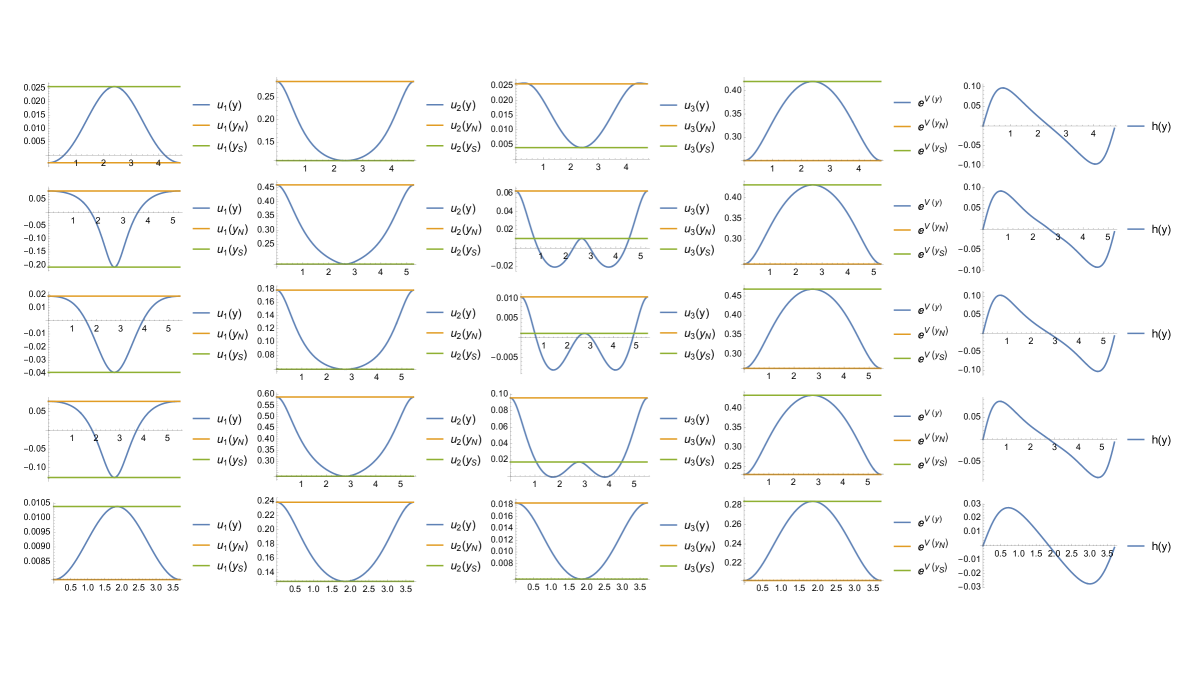
Figure 1: Numerical solutions for the scalar fields $u_{1,2,3}(y)$ and the scalar functions $e^{V}(y)$ and $h(y)$ interpolating between the north pole at $y=y_{N}=0$ and $y=2(y_{S}-y_{N})$, where $y_{S}$ is the south pole.. Each line in the plot is associated to one of the first five lines in the table (78), where the values of $n_{S},n_{N}$ and $p_{F}$ are specified. These values are explicitly $(n_{S},n_{N},p_{F})=(7,1,1)$ for the first line, $(9,1,2)$ for the second line, $(11,1,1)$ for the third line, $(11,1,3)$ for the fourth line, and $(9,3,1)$ for the fifth line.

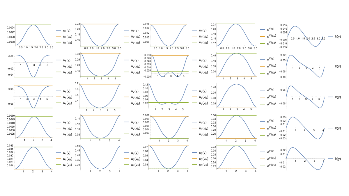
Figure 2: Numerical solutions for the scalar fields $u_{1,2,3}(y)$ and the scalar functions $e^{V}(y)$ and $h(y)$ interpolating between the north pole at $y=y_{N}=0$ and $y=2(y_{S}-y_{N})$, where $y_{S}$ is the south pole.. Each line in the plot is associated to one of the last five lines in the table (78), where the values of $n_{S},n_{N}$ and $p_{F}$ are specified. These values are explicitly $(n_{S},n_{N},p_{F})=(11,5,1)$ for the first line, $(13,1,2)$ for the second line, $(13,1,4)$ for the third line, $(13,3,1)$ for the fourth line, and $(13,3,3)$ for the fifth line.

6 Comparison with the field theory results

In this section we compare the results found above for the central charge in the anti-twist class for the conifold truncation with respect to the calculation performed in the dual field theory.

Such calculation has been performed originally in Hosseini:2021fge by integrating the anomaly polynomial over the geometry of the spindle. Such integration has been pursued thanks to the observation that the anomaly polynomial can be written as gluing formula in terms of the four dimensional conformal anomaly, formally expressed in terms of the R-charges, the deficit angles and the flavor fluxes. By c-extremization the final expression, in terms of the pole data and of the quantized fluxes, is Boido:2022mbe

$$c_{2d}=\frac{3(m_{-}+\sigma m_{+})^{2}\sum_{a<b,c\neq a,b}\mathbf{p}_{a}\mathbf{p}_{b}\mathbf{p}_{c}^{2}\cdot\sum_{a<b<c}\mathbf{p}_{a}\mathbf{p}_{b}\mathbf{p}_{c}}{(m_{-}^{2}-\sigma m_{-}m_{+}+m_{+}^{2})\prod_{a<b}(\mathbf{p}_{a}+\mathbf{p}_{b})-\sigma m_{+}m_{-}\Theta_{KW}}N^{2}$$ (79)

with

$$\Theta_{KW}=\sum_{a<b,c\neq a,b}\mathbf{p}_{a}\mathbf{p}_{b}\mathbf{p}_{c}^{4}-2\sum_{a<b}\mathbf{p}_{a}\mathbf{p}_{b}\prod_{c}\mathbf{p}_{c}.$$ (80)

The comparison with the gravitational calculation requires a further restriction on the values of the fluxes. The fluxes $\mathbf{p}_{1,2,3,4}$ are associated to the Cartan of the global $U(1)_{r}\times SU(2)_{L}\times SU(2)_{R}\times U(1)_{B}$ of the conifold. They are constrained by the relation $\mathbf{p}_{1}+\mathbf{p}_{2}+\mathbf{p}_{3}+\mathbf{p}_{4}=-\frac{m_{-}+\sigma m_{+}}{m_{-}m_{+}}$ ensuring the correct quantization for the magnetic flux associated to the R-symmetry for the twist $\sigma=1$ and the anti-twist $\sigma=-1$. The baryonic flux is instead associated to the combination $\mathbf{p}_{1}-\mathbf{p}_{2}+\mathbf{p}_{3}-\mathbf{p}_{4}$. The other global symmetries associated to the flavor symmetries are set to zero in the 5d supergravtiy model, that is indeed realized by truncating over the Reeb vector. It follows that the actual comparison requires to fix the fluxes as

$$\mathbf{p}_{1}=\mathbf{p}_{3}=-\frac{m_{-}+\sigma m_{+}}{4m_{-}m_{+}}+\frac{p_{b}}{2m_{-}m_{+}}$$ (81)

and

$$\mathbf{p}_{2}=\mathbf{p}_{4}=-\frac{m_{-}+\sigma m_{+}}{4m_{-}m_{+}}-\frac{p_{b}}{2m_{-}m_{+}}.$$ (82)

Furthermore we choose $\sigma=-1$ because we have to consider the anti-twist. Eventually we fix the pole data in the notation of Boido:2022mbe and the ones here by identifying $m_{+}=n_{N}$ and $m_{-}=n_{S}$. The central charge in formula (79) then becomes

$$c_{2d}=\frac{3N_{c}^{2}(n_{N}-n_{S})(3(n_{S}-n_{N})^{2}+p_{b}^{2})((n_{S}-n_{N})^{2}-p_{b}^{2})}{16n_{N}n_{S}(n_{N}^{4}-n_{N}n_{S}^{3}-n_{N}^{3}n_{S}+n_{S}^{4}-p_{b}^{2}n_{N}n_{S})}.$$ (83)

This expression matches (4.3) upon the identification $p_{F}=p_{b}$.

Let us conclude this section with an observation related to the relation between our results and the general discussion that appeared in Boido:2022mbe regarding the geometries of Type IIB constructed from a 5d SE and a spindle. It has been observed that such geometries are constructed by fixing only the fluxes associated to the flavor symmetries, i.e. one can always turn off the baryonic symmetry to obtain the internal Gauntlett-Kim 7d geometry Gauntlett:2007ts . We expect that the solutions found here, when uplifted to 10d are in the class of Gauntlett:2007ts , with just five-form flux turned on.

7 Conclusions

In this paper we studied a supersymmetric AdS${}_{3}\times\Sigma$ asymptotic to the AdS₅ $\mathcal{N}=2$ truncation of the conifold with a Betti vector multiplet found in Cassani:2010na . The model consists of gauged supergravity with two vector multiplets and two hypermultiplets. The vector fields gauge a subgroup of the quaternionic manifold and one gauge field becomes massive via Higgs mechanism. In the low energy spectrum there are then two massless fields, the graviphoton and the Betti vector. One is associated to the R-symmetry and the other one to the baryonic symmetry of the dual Klebanov-Witten field theory. When this model is compactified on the spindle many of the scalars in the hypermultiplet can be further truncated. A crucial aspect of this compactification is that we need to include some of the scalars from the hypermultiplet in the analysis. After a suitable ansatz on the dependence of the spindle coordinates from the scalar fields, we have computed the BPS and the gauge fields equations. This has allowed us to find the properly quantized fluxes through the spindle. We have shown that the analysis of the fluxes can be performed by studying the BPS equations at the poles of the spindle and that this analysis, in the conformal gauge, fixes the proper boundary conditions for all the scalars except the ones in the hypermultiplet. Furthermore thanks to this analysis it has been possible to compute the central charge of the would be AdS₃ solution from the Brown-Henneaux formula. By inspection we have observed that only the anti-twist class is consistent with the unitarity bound requiring a positive central charge. This analysis is however not enough to claim the existence of the AdS₃ solution and for this reason it is necessary to solve the BPS equations explicitly from the north to the south pole of the spindle. By turning off the baryonic magnetic charge we have observed that the universal solution of Ferrero:2020laf is recovered. Furthermore we have provided a numerical analysis for the case with the magnetic baryonic charge turned on. In the numerical analysis we have first imposed the boundary conditions obtained from the analysis of the BPS equations at the north pole. Then we have scanned the boundary value of the scalar in the hypermultiplet that we cannot turn off. Solving the BPS equations for various initial data we have looked for the unique solution corresponding to the existence of a compact spindle. Once this value has been found we have checked that indeed the other fields take the value expected from the analysis of the pole data at the south pole, where this last value has been extracted numerically. We have eventually compared our general expression of central charge for the anti-twist with the one obtained in Hosseini:2021fge ; Boido:2022mbe from the dual field theory, restricted to the baryonic anti-twist, and we have found an exact agreement.

Many interesting directions in the study of supergravity truncations on the spindle deserve further investigation. For example one can study other consistent 5d $\mathcal{N}=2$ truncations with vector multiplets and hypermultiplets where an holographic dual field theory is available. From the analysis performed here and previously in Boido:2022mbe one can observe that the central charge can be extracted from the pole data if the number of conserved charges $n_{q}$ is twice the number of massless vector multiplets $n_{v}^{m^{2}=0}$. We observe that $n_{v}^{m^{2}=0}=1$ because the number of conserved charges corresponds to $n_{v}^{m^{2}=0}+1$. If this is not the case then one should provide a more general solution of the BPS equations from the numerical analysis. The problem in this last case is that the boundary conditions for some of the scalars in the vector multiplets must be fixed numerically together with the ones for the scalar(s) in the hypermultiplet. Searching for such initial data is in general non-trivial and it may require a refinement of the numerical techniques. An interesting truncation that has $n_{v}^{m^{2}=0}=1$ is the one recently worked out in Cassani:2020cod elaborating on previous results Szepietowski:2012tb . This truncation describes a stack of M5 branes wrapped on a two dimensional Riemann surface $\Sigma$. In this case the holographic dual field theories have been found in Bah:2011vv ; Bah:2012dg . We expect that the compactification of this truncation on the spindle proceeds along the same lines of the discussion performed here and in Arav:2022lzo and that the central charge in this case can be extracted from the pole data as well. It should be interesting to study this case by turning on a magnetic charge for the flavor symmetry in order to obtain the solution of the BPS equations interpolating between the poles of the compact spindle. We are currently investigating in this direction.

Another interesting aspect discussed in Arav:2022lzo consists of reformulating the BPS equations in a D=4 Janus form in order to interpret the conserved charges from a different perspective. We expect that similar results can be provided for the model discussed in this paper as well.

A more complicated question regards the interpretation of the solutions found here from a flow across dimensions along the radial direction. This requires a modification of the anstaz (16) and requires to solve the BPS equations also for the radial profiles of the scalars. Finding such solutions is a necessary step to obtain a supergravity attractor mechanism dual to c-extremization on the spindle.

We conclude by observing that one can also look at truncations dual to 3d SCFT, corresponding to AdS₄ $\mathcal{N}=2$ gauged supergravity in presence of hypermultiplets. In this case an attempt has recently in Suh:2022pkg where the case of the mABJM model has been considered. In this case one has $n_{v}^{m^{2}=0}=2$ and the counting discussed above implies that the analysis at the poles does not entirely fixe the boundary conditions for the scalar fields in the vector multiplets. Similar results are expected for another truncation with a known dual field theory, corresponding to the case of massive Type IIA supergravity Guarino:2015jca .

Appendix A Matter-coupled $\mbox{$\mathcal{N}$}=2$ 5d gauged supergravity

In this appendix we summarize the general features of matter-coupled $\mbox{$\mathcal{N}$}=2$ gauged supergravities in five dimensions following the conventions of Bergshoeff:2002qk ; Bergshoeff:2004kh . The $\mbox{$\mathcal{N}$}=2$ 5d supergravity multiplet can be coupled to $n_{V}$ vector multiplets and $n_{H}$ hypermultiplets. Restricting us only to the bosonic sector, the field content of this class of theories is determined by the gravitational field $g_{\mu\nu}$, $n_{V}$ real moduli $\phi^{x}$ belonging to vector multiples with $x=1,\dots,n_{V}$, $4n_{H}$ real scalars (or hyperscalars) $q^{X}$ from the hypermultiplets with $X=1,\dots,4n_{H}$ and $n_{V}+1$ vector fields $A^{I}_{\mu}=(A_{\mu}^{0},A_{\mu}^{x})$ with $I=(0,x)$. The vector $A_{\mu}^{0}$ belongs to the supergravity multiplet and it is usually called the graviphoton; the vectors $A_{\mu}^{x}$ are included in the vector multiplets.

Let’s briefly discuss the properties of the $\mbox{$\mathcal{N}$}=2$ moduli space. The scalars $\phi^{x}$ parametrize a $n_{V}$-dimensional Very Special Real manifold. This scalar geometry can be defined firstly introducing a $(n_{V}+1)$-dimensional embedding manifold parameterized by the homogeneous coordinates $h^{I}(\phi^{x})$. Secondly considering the hypersurface identified by the fundamental cubic polynomial,

$$P(h)=C_{IJK}h^{I}h^{J}h^{K}=1\,,$$ (84)

where $C_{IJK}$ is a constant and symmetric tensor. From the tensor $C_{IJK}$ and the homogeneous coordinates $h^{I}$ is thus possible to derive all the quantities needed to describe the couplings to vector multiplets. In fact on such hypersurface we can introduce a metric $g_{xy}$ as the pull-back of the metric $a_{IJ}$ on the embedding space,

$$g_{xy}=\frac{3}{2}\partial_{x}h^{I}\partial_{y}h^{J}\,a_{IJ}\qquad\text{with}\qquad a_{IJ}=-\frac{1}{3}\,\partial_{h^{I}}\partial_{h^{J}}\,\log P(h)|_{P=1}\,.$$ (85)

The coupling between scalars $\phi^{x}$ and vectors $A^{I}_{\mu}$ is realized through the metric $a_{IJ}$ which can be alternatively defined as

$$a_{IJ}=-2C_{IJK}h^{K}+3h_{I}h_{J}\qquad\text{with}\qquad h_{I}\equiv a_{IJ}h^{J}=C_{IJK}h^{J}h^{K}\,.$$ (86)

The hyperscalars $q^{X}$ parametrize a Quaternionic manifold which can be defined as a Riemannian manifold with metric $g_{XY}$ endowed with a locally defined triplet $\vec{J}_{XY}$ of almost complex structures satisfying the relations

$$\begin{split}&g^{ZW}\,J^{r}_{XZ}J^{s}_{WY}=-\delta^{rs}g_{XY}+\varepsilon^{rst}J^{t}_{XY}\,,\\ &\widetilde{\nabla}_{Z}\vec{J}_{X}^{\ \,Y}=\nabla_{Z}\vec{J}_{X}^{\ \,Y}+2\,\vec{\omega}_{Z}\times\vec{J}_{X}^{\ \,Y}=0\end{split}$$ (87)

where $\{r,s,t\}=1,2,3$ are indices of the vectorial representation of $SU(2)$. The first expression in (LABEL:quaternionicrelations) is the defining relation of a quaternionic structure. The second implies that $\vec{J}$ is covariantly constant w.r.t. the connection $\vec{\omega}=\vec{\omega}_{X}(q)dq^{X}$ associated to a $SU(2)$-bundle defined over the quaternionic manifold. The corresponding $SU(2)$-curvature $\vec{\mbox{$\mathcal{R}$}}$ turns out to be proportional to the complex structures $\vec{J}_{XY}$ as it follows

$$\vec{\mbox{$\mathcal{R}$}}=d\vec{\omega}+2\,\vec{\omega}\wedge\vec{\omega}=\frac{1}{2}\,\nu\vec{J}\,\qquad\text{with}\qquad\nu\equiv\frac{1}{4n_{H}(n_{H}+2)}\,R.$$ (89)

In this paper we focus only on abelian gaugings on the quaternionic manifold. These are typically generated by commuting Killing vectors $k_{I}^{X}(q)$. For each Killing vector we can introduce a triplet of moment maps $\vec{P}_{I}$ through the relation

$$\begin{split}&\widetilde{\nabla}_{X}\vec{P}_{I}=\partial_{X}\vec{P}_{I}+2\,\vec{\omega}_{X}\times\vec{P}_{I}=\vec{J}_{XY}k^{Y}_{I}\,.\\ \end{split}$$ (90)

We are now ready to write the bosonic Lagrangian,

$$\begin{split}e^{-1}\mathscr{L}=&\,\,\frac{1}{2}R-\frac{1}{2}g_{xy}(\phi)\partial_{\mu}\phi^{x}\partial^{\mu}\phi^{y}-\frac{1}{2}g_{XY}(q)\mathcal{D}_{\mu}q^{X}\mathcal{D}^{\mu}q^{Y}-\frac{1}{4}a_{IJ}(\phi)F^{I}_{\mu\nu}F^{J\,\mu\nu}\\ &+\frac{e^{-1}}{12}\sqrt{\frac{2}{3}}C_{IJK}\epsilon^{\mu\nu\rho\sigma\tau}F^{I}_{\mu\nu}F^{J}_{\rho\sigma}A^{K}_{\tau}-g^{2}V(\phi,q),\end{split}$$ (91)

where

$$\mathcal{D}_{\mu}q^{u}=\partial_{\mu}q^{u}+gA^{I}_{\mu}k^{u}_{I}$$ (92)

are the covariant derivatives of hyperscalars depending on the gauge coupling $g$. Finally the scalar potential $V(\phi,q)$ has the form

$$\begin{split}V=&P_{I}^{r}P_{J}^{r}\Bigl{(}4h^{I}h^{J}-3g^{xy}\partial_{x}h^{I}\partial_{y}h^{J}\Bigr{)}-\frac{3}{4}g_{XY}k_{I}^{X}k_{J}^{Y}h^{I}h^{J}\,.\end{split}$$ (93)

We point out that since the gauging is abelian, the coviarant derivatives of the scalars $\phi^{x}$ are just the ordinary onces since the scalars $\phi^{x}$ transform trivially under abelian symmetries.

Finally we can write the $\mbox{$\mathcal{N}$}=2$ supersymmetry variations using the conventions of Bergshoeff:2004kh ; Halmagyi:2011yd ; Louis:2016msm . Given a $\mbox{$\mathcal{N}$}=2$ Killing spinor $\epsilon^{i}$, the fermionic variations have the following form

$$\delta\psi_{\mu}^{i} =\bigl{[}D_{\mu}+\frac{i}{4\sqrt{6}}h_{I}(\gamma_{\mu}^{\ \nu\rho}-4\delta_{\mu}^{\nu}\gamma^{\rho})F^{I}_{\nu\rho}\bigr{]}\epsilon^{i}-\frac{i}{\sqrt{6}}g\,\gamma_{\mu}h^{I}(P_{I})^{ij}\epsilon_{j},$$ (94)

$$\delta\lambda^{x\,i} =\bigl{(}-\frac{i}{2}\gamma^{\mu}\partial_{\mu}\phi^{x}+\frac{1}{4}\gamma^{\mu\nu}F^{I}_{\mu\nu}h^{x}_{I}\bigr{)}\epsilon^{i}-g\,P^{x\,ij}\epsilon_{j},$$ (95)

$$\delta\zeta^{A} =\frac{i}{2}\gamma^{\mu}\mathcal{D}_{\mu}q^{X}f^{iA}_{X}\epsilon_{i}-\frac{\sqrt{6}\,g}{4}h^{I}\,k_{I}^{X}f^{iA}_{X}\epsilon_{i},$$ (96)

where we have introduced the quaternionic vielbein $f^{iA}_{X}$ Bergshoeff:2004kh and the supercovariant derivative

$$\begin{split}&D_{\mu}\epsilon^{i}=\partial_{\mu}\epsilon^{i}+\frac{1}{4}\omega^{ab}_{\mu}\gamma_{ab}\epsilon^{i}-\partial_{\mu}q^{X}\omega^{ij}_{X}\epsilon_{j}-gA_{\mu}^{I}P_{I}^{ij}\epsilon_{j}\,,\\ \end{split}$$ (97)

acting on the supersymmetry parameter $\epsilon^{i}$.
The vielbein $f^{iA}_{X}$ satisfies the following relation with the almost complex structures:

$$i\,\vec{J}_{X}^{\ \,Y}\cdot\vec{\sigma}_{i}^{\ j}=2f_{X}^{jA}f^{Y}_{iA}-\delta_{i}^{j}\delta_{X}^{Y},$$ (98)

that will be useful in the simplification of the BPS equations.

Appendix B Details on the quaternionic geometry

In this appendix we derive the quaternionic structures $\vec{J}$ and the $SU(2)$ spin connections $\vec{\omega}$ for the quaternionic manifold

$$\frac{SO(4,2)}{SO(4)\times SO(2)}.$$ (99)

This scalar geometry was already studied in detail in Halmagyi:2011yd ; Louis:2016msm ; DallAgata:2021nnr and it is described by $n_{H}=2$ hypermultiplets, whose real scalars can be organized as $q^{X},\ X=1,\dots,8$

Following Halmagyi:2011yd ; Louis:2016msm we use the coordinates $q^{X}=\{u_{1},k,a,\phi,b^{1},\bar{b}^{1},b^{2},\bar{b}^{2}\}$, with line element given by

$$\begin{split}g_{XY}dq^{X}dq^{Y}=&-2e^{-4u_{1}}M_{ij}\bigl{(}b^{i}d\bar{b}^{j}+\bar{b}^{i}db^{j}\bigr{)}-4du_{1}^{2}-\frac{1}{4}d\phi^{2}-\frac{1}{4}e^{2\phi}da^{2}\\ &-\frac{1}{4}e^{-8u_{1}}\Bigl{[}dk+2\varepsilon_{ij}\bigl{(}b^{i}d\bar{b}^{j}+\bar{b}^{i}db^{j}\bigr{)}\Bigr{]}^{2},\end{split}$$ (100)

where

$$M_{ij}=e^{\phi}\begin{pmatrix}a^{2}+e^{-2\phi}&\quad-a\\ -a&1\end{pmatrix}.$$ (101)

We have chosen the normalization of the metric in order to have the curvature scalar $R=64$ and thus $\vec{\mathcal{R}}=\vec{J}$ (see (89)). This last equality is necessary to obtain the simplified version of the hyperino variation in (125).

To display the quaternionic structure of the coset, we follow the explicit construction made in Appendix E of Cheung:2021igt , adapting it to our coordinates, and we introduce the quaternionic vielbeins

$$\begin{split}f^{1}&=\frac{i}{2}d\phi,\qquad f^{2}=2i\,du_{1},\qquad f^{3}=\frac{i}{2}e^{\phi}da,\\ f^{4}&=ie^{-4u_{1}}\biggl{(}\frac{1}{2}dk-\bar{b}^{2}db^{1}+\bar{b}^{1}db^{2}-b^{2}d\bar{b}^{1}+b^{1}d\bar{b}^{2}\biggr{)},\\ f^{5}&=\frac{i}{\sqrt{2}}e^{-2u_{1}-\frac{\phi}{2}}\bigl{(}db^{1}+d\bar{b}^{1}\bigr{)},\qquad f^{6}=\frac{1}{\sqrt{2}}e^{-2u_{1}-\frac{\phi}{2}}\bigl{(}db^{1}-d\bar{b}^{1}\bigr{)},\\ f^{7}&=\frac{i}{\sqrt{2}}e^{-2u_{1}+\frac{\phi}{2}}\bigl{(}-a\,db^{1}+db^{2}-a\,d\bar{b}^{1}+d\bar{b}^{2}\bigr{)},\\ f^{8}&=-\frac{1}{\sqrt{2}}e^{-2u_{1}+\frac{\phi}{2}}\bigl{(}a\,db^{1}-db^{2}+a\,d\bar{b}^{1}-d\bar{b}^{2}\bigr{)}.\end{split}$$ (102)

We can thus obtain the triplet of almost complex structures $\vec{J}$ as

$$\begin{split}J^{1}&=\frac{1}{\sqrt{2}}\Bigl{(}f^{15}+f^{18}+f^{25}-f^{28}-f^{36}+f^{37}-f^{46}-f^{47}\Bigr{)},\\ J^{2}&=\frac{1}{\sqrt{2}}\Bigl{(}f^{16}-f^{17}+f^{26}+f^{27}+f^{35}+f^{38}+f^{45}-f^{48}\Bigr{)},\\ J^{3}&=-\Bigl{(}f^{13}+f^{24}+f^{56}+f^{78}\Bigr{)},\end{split}$$ (103)

where $f^{ij}\equiv f^{i}\wedge f^{j}$ and $J^{r}=\frac{1}{2}J^{r}_{\ XY}\,dq^{X}\wedge dq^{Y}$ for $r=1,2,3$. One can check that these structures satisfy the quaternionic relations in (LABEL:quaternionicrelations). In this setting, the $SU(2)$ connections take the form

$$\begin{split}\omega^{1}&=\frac{1}{2}e^{-2u_{1}-\frac{\phi}{2}}(db^{1}+d\bar{b}^{1})-\frac{i}{2}a\,e^{-2u_{1}+\frac{\phi}{2}}(db^{1}-d\bar{b}^{1})+\frac{i}{2}e^{-2u_{1}+\frac{\phi}{2}}(db^{2}-d\bar{b}^{2}),\\ \omega^{2}&=-\frac{i}{2}e^{-2u_{1}-\frac{\phi}{2}}(db^{1}-d\bar{b}^{1})-\frac{1}{2}a\,e^{-2u_{1}+\frac{\phi}{2}}(d\bar{b}^{1}+d\bar{b}^{1})+\frac{1}{2}e^{-2u_{1}+\frac{\phi}{2}}(db^{2}+d\bar{b}^{2}),\\ \omega^{3}&=\frac{1}{4}e^{\phi}da-\frac{1}{2}e^{-4u_{1}}\biggl{(}\frac{1}{2}dk-\bar{b}^{2}db^{1}+\bar{b}^{1}db^{2}-b^{2}d\bar{b}^{1}+b^{1}d\bar{b}^{2}\biggr{)}.\end{split}$$ (104)

Appendix C Derivation of the BPS equations

Following the analysis made in Arav:2022lzo , in order to construct AdS${}_{3}\times\Sigma$ solutions to the BPS equations, we first decompose the Clifford algebra via

$$\gamma^{m}=\Gamma^{m}\otimes\sigma^{3},\qquad\gamma^{3}=\mathbb{I}_{2}\otimes\sigma^{1},\qquad\gamma^{4}=\mathbb{I}_{2}\otimes\sigma^{2},$$ (105)

where $\Gamma^{m}=\bigl{(}-i\sigma^{2},\sigma^{3},\sigma^{1}\bigr{)}$ are the gamma matrices in $d=3$ and $\sigma^{i},\ i=1,2,3,$ are the Pauli matrices. We can thus write the Killing spinor as

$$\epsilon=\psi\otimes\chi,$$ (106)

where $\chi$ is a two-component spinor on the spindle and $\psi$ is a two-component spinor on AdS₃ satisfying

$$\nabla_{m}\psi=-\frac{\kappa}{2}\,\Gamma_{m}\psi,$$ (107)

where $\kappa=\pm 1$ specifies the chirality of the supersymmetry of the dual 2d SCFT. In this section we will analyze the BPS equations in order to determine the structure of the spinor $\chi$, that is given by

$$\chi=e^{V/2}e^{isz}\begin{pmatrix}\sin\frac{\xi}{2}\\ \cos\frac{\xi}{2}\end{pmatrix}$$ (108)

as we will see in more detail in a few.

C.1 Gravitino variation

The supersymmetry variation for the gravitino in (94) splits into two decoupled equations if we impose the projection condition on the symplectic-Majorana $\epsilon^{i}$ . This decoupling is due to the fact that in our model only the $r=3$ $SU(2)$-components of the moment maps survive (see (13)), which are related to the doublet notation through the third Pauli matrix via (88).
Thus, one of the two BPS equations obtained from the gravitino variation can be written as

$$\delta\psi_{\mu}=\Bigl{[}\nabla_{\mu}-iQ_{\mu}+\frac{i}{12}H_{\nu\rho}\bigl{(}\gamma^{\nu\rho}\gamma_{\mu}+2\gamma^{\nu}\delta_{\mu}^{\rho}\bigr{)}+\frac{1}{2}gW\gamma_{\mu}\Bigr{]}\epsilon=0,$$ (109)

where $\epsilon$ is now a Dirac spinor, $\nabla_{\mu}\epsilon=\partial_{\mu}\epsilon+\frac{1}{4}\omega_{\mu ab}\gamma^{ab}$ and $Q_{\mu}\equiv\partial_{\mu}q^{X}\omega_{X}^{3}+gA_{\mu}^{I}P_{I}^{3}$. We also introduced the superpotential $W\equiv\sqrt{\frac{2}{3}}h^{I}P_{I}^{3}$ and $H_{\mu\nu}\equiv h_{I}F^{I}_{\mu\nu}$.
The components of (109) that are tangent to the directions along AdS₃ give:

$$\bigl{[}-\bigl{(}\kappa e^{-V}+\frac{1}{\sqrt{6}}H_{34}\bigr{)}\gamma^{34}+i\,V^{\prime}f^{-1}\gamma^{3}\bigr{]}\epsilon=-igW\epsilon.$$ (110)

In order to have non-trivial solutions to this equation, we have to impose that the two coefficients on the left hand side live on a circle, i.e.

$$\bigl{[}\cos\xi\gamma^{34}+i\sin\xi\gamma^{3}\bigr{]}\epsilon=-i\epsilon.$$ (111)

This projection condition is solved by

$$\epsilon=e^{-i\frac{\xi}{2}\gamma^{4}}\eta,\qquad\gamma^{3}\eta=i\gamma^{4}\eta$$ (112)

and it allows us to split (110) in

$$-\kappa e^{-V}-\frac{1}{\sqrt{6}}H_{34}=gW\cos\xi,\qquad V^{\prime}f^{-1}=gW\sin\xi.$$ (113)

If we now focus on the component of the gravitino variation in the longitudinal direction of the spindle, i.e. $\mu=y$, we can rewrite it as

$$\Bigl{[}\partial_{y}-\frac{1}{2}V^{\prime}-\frac{i}{2}\bigl{(}\partial_{y}\xi+\sqrt{\frac{3}{2}}fH_{34}+\kappa fe^{-V}\bigr{)}\gamma^{4}\Bigr{]}\eta=0.$$ (114)

One can notice that this expression is in the form $(a_{1}+a_{2}\gamma^{4})\eta=0$, which implies that $a_{1}^{2}+a_{2}^{2}=0$.
Therefore, from the first part of (114) we can infer that $\eta$ has the structure

$$\eta=e^{V/2}e^{isz}\eta_{0},$$ (115)

where $s$ is a constant and $\eta_{0}$ is independent from $y$ and $z$. From the second part of (114) we obtain

$$\partial_{y}\xi+\sqrt{\frac{3}{2}}fH_{34}+\kappa fe^{-V}=0.$$ (116)

Similarly, the component along the azimuthal direction of the spindle ($\mu=z$) gives

$$\begin{split}\Bigl{[}\partial_{z}-iQ_{z}&+\frac{i}{2}f^{-1}h^{\prime}\cos\xi-\frac{i}{\sqrt{6}}H_{34}h\sin\xi\\ &+\Bigl{(}-\frac{1}{2}f^{-1}h^{\prime}\sin\xi+\frac{1}{2}gWh-\frac{1}{\sqrt{6}}H_{34}h\cos\xi\Bigr{)}\gamma^{4}\Bigr{]}\eta=0,\end{split}$$ (117)

from which

$$(s-Q_{z})+\frac{1}{2}f^{-1}h^{\prime}\cos\xi-\frac{1}{\sqrt{6}}H_{34}h\sin\xi=0,$$ (118)

$$-\frac{1}{2}f^{-1}h^{\prime}\sin\xi+\frac{gWh}{2}-\frac{1}{\sqrt{6}}H_{34}h\cos\xi=0.$$ (119)

C.2 Gaugino variation

Using some relations of the Very Special Real geometry and the definition of the superpotential, the variation of the gaugino (95) gives

$$\delta\lambda^{x}=\Bigl{[}-\frac{i}{2}\gamma^{\mu}\partial_{\mu}\phi^{x}+\frac{1}{4}\sqrt{\frac{3}{2}}g^{xy}\partial_{y}h_{I}\gamma^{\mu\nu}F^{I}_{\mu\nu}+i\sqrt{\frac{3}{2}}g\,g^{xy}\partial_{y}W\Bigr{]}\epsilon=0.$$ (120)

From the first component ($x=1$), imposing again the projection condition in (111), we obtain

$$f^{-1}u_{2}^{\prime}+\frac{3g}{4}\partial_{u_{2}}W\sin\xi=0,$$ (121)

$$3g\,\partial_{u_{2}}W\cos\xi+\sqrt{\frac{2}{3}}e^{2u_{3}}\bigl{(}e^{-2u_{2}}F_{34}^{(1)}-e^{2u_{2}}F_{34}^{(2)}\bigr{)}=0,$$ (122)

where we have used the explicit expressions for the sections $h^{I}$ and for the field strengths. Similarly, from the component $x=2$, we have

$$f^{-1}u_{3}^{\prime}+\frac{g}{4}\partial_{u_{3}}W\sin\xi=0,$$ (123)

$$3g\,\partial_{u_{3}}W\cos\xi+\sqrt{\frac{2}{3}}\bigl{(}2e^{-4u_{3}}F_{34}^{(0)}-e^{-2u_{2}+2u_{3}}F_{34}^{(1)}-e^{2u_{2}+2u_{3}}F_{34}^{(2)}\bigr{)}=0.$$ (124)

C.3 Hyperino variation

In order to simplify the BPS equation coming from the hyperino variation in (96), we can multiply its expression for $f_{jAY}$. Using (98), after some calculations we obtain the relation

$$\Bigl{(}2i\gamma^{\mu}\partial_{\mu}u_{1}+\frac{3}{8}ig\partial_{u_{1}}W+\frac{1}{4}\partial_{u_{1}}Q_{\mu}\gamma^{\mu}\Bigr{)}\epsilon=0.$$ (125)

Notice that to single out the vector $Q_{\mu}$, introduced in (109), it is necessary to make a precise choice of the normalization of the metric of the quaternionic manifold, as we have pointed out in appendix B.
Finally, imposing the projection condition (111), this last equation gives

$$f^{-1}u_{1}^{\prime} =\frac{3g}{16}\frac{\partial_{u_{1}}W}{\sin\xi},$$ (126)

$$\frac{3g}{2}\partial_{u_{1}}W\cos\xi =h^{-1}\partial_{u_{1}}Q_{z}\sin\xi.$$ (127)

References

- (1) E. Witten, Topological Sigma Models, Commun. Math. Phys. 118 (1988) 411.
- (2) M. Bershadsky, A. Johansen, V. Sadov and C. Vafa, Topological reduction of 4-d SYM to 2-d sigma models, Nucl. Phys. B 448 (1995) 166 [hep-th/9501096].
- (3) M. Bershadsky, C. Vafa and V. Sadov, D-branes and topological field theories, Nucl. Phys. B 463 (1996) 420 [hep-th/9511222].
- (4) J. M. Maldacena and C. Nunez, Supergravity description of field theories on curved manifolds and a no go theorem, Int. J. Mod. Phys. A 16 (2001) 822 [hep-th/0007018].
- (5) F. Benini and N. Bobev, Two-dimensional SCFTs from wrapped branes and c-extremization, JHEP 06 (2013) 005 [1302.4451].
- (6) F. Benini and N. Bobev, Exact two-dimensional superconformal R-symmetry and c-extremization, Phys. Rev. Lett. 110 (2013) 061601 [1211.4030].
- (7) P. Ferrero, J. P. Gauntlett, J. M. Pérez Ipiña, D. Martelli and J. Sparks, D3-Branes Wrapped on a Spindle, Phys. Rev. Lett. 126 (2021) 111601 [2011.10579].
- (8) P. Ferrero, J. P. Gauntlett and J. Sparks, Supersymmetric spindles, JHEP 01 (2022) 102 [2112.01543].
- (9) P. Ferrero, J. P. Gauntlett, J. M. P. Ipiña, D. Martelli and J. Sparks, Accelerating black holes and spinning spindles, Phys. Rev. D 104 (2021) 046007 [2012.08530].
- (10) S. M. Hosseini, K. Hristov and A. Zaffaroni, Rotating multi-charge spindles and their microstates, JHEP 07 (2021) 182 [2104.11249].
- (11) A. Boido, J. M. P. Ipiña and J. Sparks, Twisted D3-brane and M5-brane compactifications from multi-charge spindles, JHEP 07 (2021) 222 [2104.13287].
- (12) P. Ferrero, J. P. Gauntlett, D. Martelli and J. Sparks, M5-branes wrapped on a spindle, JHEP 11 (2021) 002 [2105.13344].
- (13) P. Ferrero, M. Inglese, D. Martelli and J. Sparks, Multicharge accelerating black holes and spinning spindles, Phys. Rev. D 105 (2022) 126001 [2109.14625].
- (14) C. Couzens, K. Stemerdink and D. van de Heisteeg, M2-branes on discs and multi-charged spindles, JHEP 04 (2022) 107 [2110.00571].
- (15) F. Faedo and D. Martelli, D4-branes wrapped on a spindle, JHEP 02 (2022) 101 [2111.13660].
- (16) S. Giri, Black holes with spindles at the horizon, JHEP 06 (2022) 145 [2112.04431].
- (17) C. Couzens, A tale of (M)2 twists, JHEP 03 (2022) 078 [2112.04462].
- (18) P. Karndumri and P. Nuchino, Five-branes wrapped on topological disks from 7D N=2 gauged supergravity, Phys. Rev. D 105 (2022) 066010 [2201.05037].
- (19) K. C. M. Cheung and R. Leung, Type IIA embeddings of D = 5 minimal gauged supergravity via non-Abelian T-duality, JHEP 06 (2022) 051 [2203.15114].
- (20) K. C. M. Cheung, J. H. T. Fry, J. P. Gauntlett and J. Sparks, M5-branes wrapped on four-dimensional orbifolds, JHEP 08 (2022) 082 [2204.02990].
- (21) C. Couzens, H. Kim, N. Kim and Y. Lee, Holographic duals of M5-branes on an irregularly punctured sphere, JHEP 07 (2022) 102 [2204.13537].
- (22) M. Suh, M5-branes and D4-branes wrapped on a direct product of spindle and Riemann surface, 2207.00034.
- (23) C. Couzens and K. Stemerdink, Universal spindles: D2’s on and M5’s on , 2207.06449.
- (24) C. Couzens, N. T. Macpherson and A. Passias, A plethora of Type IIA embeddings for minimal supergravity, 2209.15540.
- (25) C. Couzens, H. Kim, N. Kim, Y. Lee and M. Suh, D4-branes wrapped on four-dimensional orbifolds through consistent truncation, 2210.15695.
- (26) F. Faedo, A. Fontanarossa and D. Martelli, Branes wrapped on orbifolds and their gravitational blocks, 2210.16128.
- (27) A. Boido, J. P. Gauntlett, D. Martelli and J. Sparks, Gravitational Blocks, Spindles and GK Geometry, 2211.02662.
- (28) M. Suh, Towards mass-deformed ABJM compactified on a spindle, 2211.11782.
- (29) M. Inglese, D. Martelli and A. Pittelli, The Spindle Index from Localization, 2303.14199.
- (30) M. Suh, Baryonic spindles from conifolds, 2304.03308.
- (31) N. Bobev, K. Pilch and O. Vasilakis, (0, 2) SCFTs from the Leigh-Strassler fixed point, JHEP 06 (2014) 094 [1403.7131].
- (32) I. Arav, J. P. Gauntlett, M. M. Roberts and C. Rosen, Leigh-Strassler compactified on a spindle, JHEP 10 (2022) 067 [2207.06427].
- (33) D. Cassani and A. F. Faedo, A Supersymmetric consistent truncation for conifold solutions, Nucl. Phys. B 843 (2011) 455 [1008.0883].
- (34) N. Halmagyi, J. T. Liu and P. Szepietowski, On = 2 Truncations of IIB on , JHEP 07 (2012) 098 [1111.6567].
- (35) F. Benini, N. Bobev and P. M. Crichigno, Two-dimensional SCFTs from D3-branes, JHEP 07 (2016) 020 [1511.09462].
- (36) A. Amariti and C. Toldo, Betti multiplets, flows across dimensions and c-extremization, JHEP 07 (2017) 040 [1610.08858].
- (37) B. S. Acharya, J. M. Figueroa-O’Farrill, C. M. Hull and B. J. Spence, Branes at conical singularities and holography, Adv. Theor. Math. Phys. 2 (1999) 1249 [hep-th/9808014].
- (38) J. P. Gauntlett and O. Varela, Universal Kaluza-Klein reductions of type IIB to N=4 supergravity in five dimensions, JHEP 06 (2010) 081 [1003.5642].
- (39) D. Cassani, G. Dall’Agata and A. F. Faedo, Type IIB supergravity on squashed Sasaki-Einstein manifolds, JHEP 05 (2010) 094 [1003.4283].
- (40) J. T. Liu, P. Szepietowski and Z. Zhao, Consistent massive truncations of IIB supergravity on Sasaki-Einstein manifolds, Phys. Rev. D 81 (2010) 124028 [1003.5374].
- (41) K. Skenderis, M. Taylor and D. Tsimpis, A Consistent truncation of IIB supergravity on manifolds admitting a Sasaki-Einstein structure, JHEP 06 (2010) 025 [1003.5657].
- (42) I. Bena, G. Giecold, M. Grana, N. Halmagyi and F. Orsi, Supersymmetric Consistent Truncations of IIB on , JHEP 04 (2011) 021 [1008.0983].
- (43) J. T. Liu and P. Szepietowski, Supersymmetry of consistent massive truncations of IIB supergravity, Phys. Rev. D 85 (2012) 126010 [1103.0029].
- (44) J. Louis and C. Muranaka, AdS5 vacua from type IIB supergravity on , JHEP 06 (2017) 035 [1611.02982].
- (45) G. Dall’Agata, M. Emelin, F. Farakos and M. Morittu, The unbearable lightness of charged gravitini, JHEP 10 (2021) 076 [2108.04254].
- (46) F. Benini, E. Colombo, S. Soltani, A. Zaffaroni and Z. Zhang, Superconformal indices at large and the entropy of AdS5 SE5 black holes, Class. Quant. Grav. 37 (2020) 215021 [2005.12308].
- (47) A. Buchel and J. T. Liu, Gauged supergravity from type IIB string theory on Y**p,q manifolds, Nucl. Phys. B 771 (2007) 93 [hep-th/0608002].
- (48) J. P. Gauntlett and O. Varela, Consistent Kaluza-Klein reductions for general supersymmetric AdS solutions, Phys. Rev. D 76 (2007) 126007 [0707.2315].
- (49) J. P. Gauntlett and N. Kim, Geometries with Killing Spinors and Supersymmetric AdS Solutions, Commun. Math. Phys. 284 (2008) 897 [0710.2590].
- (50) D. Cassani, G. Josse, M. Petrini and D. Waldram, = 2 consistent truncations from wrapped M5-branes, JHEP 02 (2021) 232 [2011.04775].
- (51) P. Szepietowski, Comments on a-maximization from gauged supergravity, JHEP 12 (2012) 018 [1209.3025].
- (52) I. Bah, C. Beem, N. Bobev and B. Wecht, AdS/CFT Dual Pairs from M5-Branes on Riemann Surfaces, Phys. Rev. D 85 (2012) 121901 [1112.5487].
- (53) I. Bah, C. Beem, N. Bobev and B. Wecht, Four-Dimensional SCFTs from M5-Branes, JHEP 06 (2012) 005 [1203.0303].
- (54) A. Guarino, D. L. Jafferis and O. Varela, String Theory Origin of Dyonic N=8 Supergravity and Its Chern-Simons Duals, Phys. Rev. Lett. 115 (2015) 091601 [1504.08009].
- (55) E. Bergshoeff, S. Cucu, T. De Wit, J. Gheerardyn, R. Halbersma, S. Vandoren et al., Superconformal N=2, D = 5 matter with and without actions, JHEP 10 (2002) 045 [hep-th/0205230].
- (56) E. Bergshoeff, S. Cucu, T. de Wit, J. Gheerardyn, S. Vandoren and A. Van Proeyen, N = 2 supergravity in five-dimensions revisited, Class. Quant. Grav. 21 (2004) 3015 [hep-th/0403045].
- (57) K. C. M. Cheung and R. Leung, Wrapped NS5-branes, consistent truncations and Inönü-Wigner contractions, JHEP 09 (2021) 052 [2106.11318].
- (58) M. Baggio, N. Halmagyi, D. R. Mayerson, D. Robbins and B. Wecht, Higher Derivative Corrections and Central Charges from Wrapped M5-branes, JHEP 12 (2014) 042 [1408.2538].