Three-dimensional active turbulence in microswimmer suspensions: simulations and modelling.

Abstract

Active turbulence is a paradigmatic and fascinating example of self-organized motion at large scales occurring in active matter. We employ massive hydrodynamic simulations of suspensions of resolved model microswimmers to tackle the phenomenon in semi-diluted conditions at a mesoscopic level. We measure the kinetic energy spectrum and find that it decays as $k^{-3}$ over a range of intermediate wavenumbers. The velocity distributions are of Lévy type, a distinct difference with inertial turbulence. Furthermore, we propose a reduced order dynamical deterministic model for active turbulence, inspired to shell models for classical turbulence, whose numerical and analytical study confirms the spectrum power-law observed in the simulations and reveals hints of a non-Gaussian, intermittent, physics of active turbulence. Direct numerical simulations and modelling also agree in pointing to a phenomenological picture whereby, in the absence of an energy cascade à la Richardson forbidden by the low Reynolds number regime, it is the coupling between fluid velocity gradients and bacterial orientation that gives rise to a multiscale dynamics.

One of the most striking features of active systems is the emergence of correlated motion and structures on scales much larger than that of the single agents. Forms of self-organized motion are ubiquitarily encountered in Nature Vicsek and Zafeiris (2012), from colonies of microorganisms Kearns (2010); Darnton et al. (2010); Koch and Subramanian (2011) to flocks of birds and fish schools Ballerini et al. (2008); Herbert-Read et al. (2011). Collective motion in microbial suspensions, in particular, appears as a tangle of coherent structures, like vortices, jets, that recall those typically encountered in turbulent flows. This morphological analogy led to coin the term bacterial or active turbulence Dombrowski et al. (2004); Wolgemuth (2008); Pedley and Kessler (1992); Alert and Casademunt (2020). But what is turbulence? Borrowing a celebrated quote, it is ”hard to define, but easy to recognize when we see it!” Vallis (1999). Is, then, visual inspection enough? Certainly not, as witnessed by the consistent body of works devoted to a quantitative description of complex motion in active systems and of its relation with turbulence. Power-law decays of kinetic energy spectra over unexpectedly wide ranges of wavenumbers have been identified as a signature of turbulent behaviour in diverse systems including dense bacterial suspensions Ishikawa et al. (2011); Wensink et al. (2012), collections of ferromagnetic spinners Kokot et al. (2015), active nematics Doostmohammadi et al. (2017); Martínez-Prat et al. (2019), synthetic swimmers at interfaces Bourgoin et al. (2020), among others. Nevertheless, a universality of some kind seems to be lacking Wensink et al. (2012); Bratanov et al. (2015), unlike in classical turbulence, where Kolmogorov’s theory of the inertial range constitutes a key, unifying ingredient Frisch (1995). With the aim of analyzing multiscale interactions and energy transfer, recent studies have focused on the spectral properties of continuum models Słomka and Dunkel (2017); Linkmann et al. (2019); Carenza et al. (2020a, b); Alert et al. (2020); Rorai et al. (2022), where the active fluid is described as an effective medium, whose equations are inspired by nematodynamics Kruse et al. (2004); Giomi et al. (2008); Edwards and Yeomans (2008); Tjhung et al. (2011) and pattern formation Wensink et al. (2012); Słomka and Dunkel (2015). In all such approaches, it is surmised that the modelled system, be it a bacterial suspension or an active gel, is densely concentrated, such that the interactions among active agents are essentially excluded volume and alignment. On the other hand, in the limit of extreme dilution (i.e. for volume fractions below the onset of collective motion), it has been shown theoretically that, due to long-range hydrodynamic interactions, suspensions of extensile microswimmers (”pushers”) develop a solvent velocity field with variance anomalously growing with the volume fraction and kinetic energy spectra whose functional form can be derived analytically with a kinetic theory approach Stenhammar et al. (2017); Bárdfalvy et al. (2019); Škultéty et al. (2020). In semi-diluted conditions, hydrodynamically induced correlations engender collective motion and large-scale flows Wu and Libchaber (2000); Hernández-Ortiz et al. (2005); Leptos et al. (2009); Saintillan and Shelley (2012). In this context, power-law spectra have been measured in numerical simulations of suspensions of point-like and slender rod-like microswimmers Saintillan and Shelley (2012); Bárdfalvy et al. (2019). However, despite these few relevant exceptions, the phenomenon of active turbulence in semi-diluted situations, namely far from close packing but above the onset of collective motion, has been much less investigated and is still poorly understood from a theoretical point of view.
We perform large scale direct numerical simulations (DNS) of suspensions of pushers, where the solvent hydrodynamics is fully resolved, both from the near to the far field. We characterize the solvent velocity field in terms of its energy spectra and probability density functions (PDFs). The spectrum displays a plateau at small wavenumbers, consistently with theoretical predictions Bárdfalvy et al. (2019); Škultéty et al. (2020) for very dilute systems, followed by an algebraic decay, $k^{-3}$, signalling the presence of fluid motion on scales up to roughly half a decade larger than the microswimmer’s size. Interestingly, such a decay has been found very recently in an experimental study of three-dimensional (3D) E. Coli suspensions Liu et al. (2021). A crucial difference from classical turbulence stands out in the velocity PDFs, which are not Gaussian but present a tempered Lévy shape.
We also introduce a reduced order dynamical deterministic model of active turbulence, pertaining to the class of the so called shell models, motivated by their successful story as turbulence models Biferale (2004). Having at disposal a shell model of active turbulence allows to study the statistical properties and chaotic behaviour of a computationally and theoretically challenging phenomenon within a low number of degrees-of-freedom description, which is, to some extent, even amenable of analytical treatment, as we also prove. The analysis of the shell model reproduces the kinetic energy spectrum power-law observed in the DNS. Remarkably, the shape of the velocity variables PDFs break scale-invariance, a hallmark of intermittency. The shell model leverages a phenomenological picture, confirmed by the DNS, whereby the coupling between the fluid velocity gradients and the bacterial orientation dynamics is the mechanism responsible for the generation of flow at large scales.

The solvent hydrodynamics is simulated using a standard $D3Q19$ lattice Boltzmann method Succi (2018); Wolf-Gladow (2000); Desplat et al. (2001). The microswimmers are modelled as solid spheres of radius $R$. The momentum/torque exchange in fluid-solid coupling is ensured by the so called bounce-back-on-links algorithm Ladd (1994); Nguyen and Ladd (2002); Aidun and Clausen (2010). The swimming mechanism is introduced via a minimal implementation of the “squirmer” model Blake (1971); Ishikawa et al. (2006), whereby a non-zero tangential polar component of the axisymmetric slip velocity is imposed at the particle surface $\mathbf{u}_{s}=\frac{3}{2}V_{p}(\sin\theta+\beta\sin\theta\cos\theta)\hat{\mathbf{\theta}}$, where $\theta=\arccos(\hat{\mathbf{e}}\cdot\hat{\mathbf{r}}_{s})$ is the angle between the squirmer orientation unit vector, $\hat{\mathbf{e}}$, and the position on the particle surface, $\hat{\mathbf{r}}_{s}=\frac{\mathbf{x}_{s}-\mathbf{X}_{p}}{R}$, relative to the position of its centre of mass, $\mathbf{X}_{p}$. $\mathbf{V}_{p}=V_{p}\hat{\mathbf{e}}$ is the self-propulsion velocity and $\beta<0$ is related to the amplitude of the stress exerted by the microswimmer on the surrounding fluid. With the above prescription for the surface slip, the squirmer generates a velocity field at the position $\mathbf{x}$ that, to leading orders, takes the form

$$\mathbf{U}(\mathbf{x},t)=V_{p}\left(\frac{3}{2}\left(\frac{R}{r}\right)^{3}(\hat{\mathbf{e}}\cdot\hat{\mathbf{r}})\hat{\mathbf{r}}-\frac{1}{2}\left(\frac{R}{r}\right)^{3}\hat{\mathbf{e}}-\frac{3}{4}\beta\left(\frac{R}{r}\right)^{2}\left(3(\hat{\mathbf{e}}\cdot\hat{\mathbf{r}})^{2}-1\right)\hat{\mathbf{r}}\right)+o\left(\left(\frac{R}{r}\right)^{4}\right)$$ (1)

where $\mathbf{r}=\mathbf{x}-\mathbf{X}_{p}(t)$, $r=|\mathbf{r}|$ and $\hat{\mathbf{r}}=\frac{\mathbf{r}}{r}$. The method has been extensively tested and applied to various physical problems, including, among others, pairwise hydrodynamic interactions, the formation of polar order, clustering and sedimentation in suspensions of microswimmers Matas Navarro and Pagonabarraga (2010); Alarcón and Pagonabarraga (2013); Alarcón et al. (2017); Scagliarini and Pagonabarraga (2022).
We perform numerical simulations in triperiodic cubic box of side $L=512$ lattice points, with $N\approx 2.6\times 10^{5}$ pushers of radius $R=2.3$ lattice units (corresponding to a volume fraction of $\phi\approx 0.1$) and $\beta=-5$. The first squirming parameter is set to $B_{1}=1.5\times 10^{-3}$, so the intrinsic self-propulsion speed is $V_{p}=10^{-3}$, in lattice Boltzmann units (lbu). The kinematic viscosity is $\nu=1/6$ lbu such that the Reynolds number at the particle scale, for an isolated microswimmer, is $\text{Re}_{p}\approx 10^{-2}$.

In Fig. 1 we report the energy spectrum $E(k)=\frac{1}{2}\overline{\langle\tilde{\mathbf{u}}^{\ast}\cdot\tilde{\mathbf{u}}\rangle}$, where $\tilde{\mathbf{u}}(\mathbf{k})$ is the Fourier transform of the fluid velocity field and the overlined brackets, $\overline{\langle(\cdot)\rangle}$, indicate a surface integral on spheres of radius $k$, in spectral space, and time averaging over the statistically stationary state.

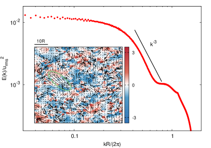
Figure 1: MAIN PANEL: Energy spectrum (time-averaged over the statistically stationary state) of the fluid velocity field, normalized by the mean square velocity $u_{\text{rms}}^{2}$, in a suspension of pushers ($\beta=-5$) at a volume fraction $\phi\approx 0.1$; the solid line indicates the scaling $E(k)\sim k^{-3}$. INSET: Snapshot of the velocity field in the plane $z=L/2$ from a simulation: the in-plane vectors $(u_{x},u_{y})$ are depicted as arrows and the out-of-plane component $u_{z}$ (rescaled by the characteristic swimming speed $V_{p}$) as a color map. Notice the size of correlated regions as compared to the microswimmer size $\sim R$; in particular, the occurrence of a jet extending on a scale of several particle radii is highlighted by the green ellipse.

The spectrum shows a plateau, $E(k)\sim\text{const}$, at small wavenumbers, followed by an algebraic decay, $E(k)\sim k^{-3}$. A constant spectrum is the theoretical expectation for an ideal system of weakly interacting point-like stresslets Stenhammar et al. (2017); Bárdfalvy et al. (2019); Škultéty et al. (2020), i.e. in the limit of extreme dilution. For finite volume fraction, the hydrodynamic interactions among particles entail a non-linear dynamics and the spectrum develops a power-law shape Saintillan and Shelley (2012); Stenhammar et al. (2017); Liu et al. (2021). Remarkably, in particular, the exponent $-3$ has been recently reported from experiments with E. Coli suspensions Liu et al. (2021) and also in previous hydrodynamic simulations with extended stresslets the energy spectrum approaches a curve consistent with $k^{-3}$ decay as the microswimmer concentration is increased from very dilute to the semi-dilute conditions Bárdfalvy et al. (2019).

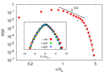
Figure 2: MAIN PANEL. Probability density function of the fluid velocity magnitude (given in units of the microswimmer intrinsic swimming speed); the solid and dashed lines highlight the algebraic decay, $u^{-5/2}$, and Gaussian tail, respectively. INSET. Probability density functions of the longitudinal velocity increments, $\delta_{l}u=\left[\mathbf{u}(\mathbf{x}+\mathbf{l},t)-\mathbf{u}(\mathbf{x},t)\right]\cdot\frac{\mathbf{l}}{l}$ (divided by their standard deviation, $\sigma_{\delta_{l}u}$), for three separations $l/R=4,30,90$. The dashed line depicts the Gaussian probability density function with zero mean and standard deviation $\sigma=1.8$.

Another peculiar aspect of the complex non-linear phenomenology of inertial turbulence is intermittency, which is intimately related to the breakup of global scale invariance Frisch (1995). Intermittency can be detected in 3D turbulent velocity fields looking at the probability density functions (PDFs) of longitudinal velocity increments $\delta_{l}u=\left[\mathbf{u}(\mathbf{x}+\mathbf{l},t)-\mathbf{u}(\mathbf{x},t)\right]\cdot\frac{\mathbf{l}}{l}$. Upon proper rescaling, such to have a fixed variance, the PDFs do not attain a scale-independent functional form: they are Gaussian when the separation is of the order of the system size, $l\sim L$ (the so called “integral scale”), but become more and more fat-tailed at decreasing $l$ (or, equivalently, the flatness grows as $l\rightarrow 0$). In contrast, in our simulations, as shown in Fig. 2 (inset), the PDFs seem to collapse onto a Gaussian curve for all $l$. Conversely, the statistics of fluid velocity, which is Gaussian in inertial turbulence, deviates substantially from Gaussianity. From the main panel of Fig. 2, we observe that the PDF of the velocity magnitude has a maximum at $u\sim V_{p}$, then goes down as $\sim u^{-5/2}$ and eventually ends up in a Gaussian tail. Overall, this shape is consistent with a tempered Lévy distribution, which is theoretically expected in suspensions of swimmers generating algebraically decaying flow fields Zaid et al. (2011). In particular, the exponent $-5/2$ stems precisely from the $U(r)\sim r^{-2}$ behaviour Rushkin et al. (2010), which dominates on long distances in our squirmer model, (see Eq. (1)). This kind of distributions were reported also from experiments with suspensions of the algae Chlamydomonas reinhardtii Leptos et al. (2009) and Volvox carteri Rushkin et al. (2010), underlining the generality of our approach.

One may wonder whether and to which extent it is possible to extend concepts and tools developed for inertial turbulence to active turbulence. To this end, we introduce a shell model for active turbulence that will generalize and rationalize the observed results. Shell models (SMs) are deterministic dynamical systems that reduce the complexity of the full (field) equations, though retaining some of their essential features. Originally introduced as a proxy of the Navier-Stokes equations, they represent a low number of degrees-of-freedom description of hydrodynamic turbulence. As such, they offer the possibility to investigate the chaotic dynamics and multiscale correlations of turbulence with obvious computational advantages  Gledzer (1973); Desnyansky and Novikov (1974); Frisch (1995); Bohr et al. (1998); Biferale (2004). Mathematically, SMs consist of a set of coupled ordinary differential equations, describing the time evolution of complex variables, $\tilde{u}_{n}(t)$ (with $n=1,2,\dots,N_{s}$), that can be thought as Fourier amplitudes of velocity fluctuations over a length scale with associated wavenumber $k_{n}$. SMs do not carry any of the geometrical information contained in the original system, as $\tilde{u}_{n}$ and $k_{n}$ are both scalar variables. $k_{n}$ stands for a radial coordinate in spectral space, whence the name shell (correspondingly, the discrete index $n$ is called shell index). Recently, SMs have been extended to polymeric solutions, to address drag reduction and elastic turbulence Benzi et al. (2003, 2004); Ray and Vincenzi (2016). Hydrodynamic theories describe active suspensions in terms of the bacteria concentration field, $c(\mathbf{x},t)$, the (incompressible) fluid velocity field, $\mathbf{u}(\mathbf{x},t)$, and an order parameter quantifying the degree of local orientation $\mathbf{P}(\mathbf{x},t)$, which represents the average, within a fluid element, of the particle intrinsic swimming director, $P_{i}\propto\langle\hat{e}_{i}\rangle$, If we assume, for simplicity, that the microswimmers spatial distribution remains homogeneous in time ($c(\mathbf{x},t)\approx c_{0}$, which is indeed confirmed by the DNS), the equations of motion read Aditi Simha and Ramaswamy (2002); Hatwalne et al. (2004); Saintillan and Shelley (2008a, b); Baskaran and Marchetti (2009),

$$\rho(\partial_{t}\mathbf{u}+\mathbf{u}\cdot\nabla)\mathbf{u} =-\nabla p+\eta\nabla^{2}\mathbf{u}+\nabla\cdot\mathbf{\sigma}^{(a)}$$

$$\partial_{t}\mathbf{P}+(\mathbf{u}+w\mathbf{P})\cdot\nabla\mathbf{P} =\mathbf{\Omega}\cdot\mathbf{P}-\Gamma\mathbf{P}+D\nabla^{2}\mathbf{P};$$ (2)

$\sigma^{(a)}_{ij}=\zeta P_{i}P_{j}$ Hatwalne et al. (2004) is the active stress, where $\zeta$ is proportional to the swimmers’ volume fraction and to the amplitude of the generated stresslet and, therefore, quantifies the level of activity. $\Omega_{ij}=\frac{1}{2}(\partial_{i}u_{j}-\partial_{j}u_{i})$ denotes the antisymmetric part of the velocity gradient tensor, and $\eta$ and $D$ are the fluid dynamic viscosity and the orientation field diffusion coefficient, respectively. Except for the term $w(\mathbf{P}\cdot\nabla)\mathbf{P}$, Eqs. (.1) closely resemble the Oldroyd-B equations for the polymer conformation Bird et al. (1987), in vectorial form Benzi et al. (2003). Inspired by this formal analogy, we propose the following shell model for active fluids (see the Supplemental Material for further details), that couples the dynamics of $u_{n}$ (we omit hereafter the tilde $\tilde{(\dots)}$, for the sake of lightening the notation) with an equation for $P_{n}$, the amplitude of orientation magnitude fluctuations at the wavenumber $k_{n}$:

$$\dot{u}_{n} =-\gamma_{u}(k_{n})u_{n}+i\zeta k_{n}P_{n}^{2}$$

$$\dot{P}_{n} =\frac{i}{3}\Phi^{(\varepsilon_{f})}_{n}(u,P)+\frac{i}{3}w\Phi^{(\varepsilon_{f})}_{n}(P,P)-\frac{i}{3}\Phi^{(\varepsilon_{b})}_{n}(P,u)$$

$$-\gamma_{P}(k_{n})P_{n}-\Gamma P_{n}+\delta_{n,n_{B}}|P_{n}|^{-1}P_{n}P_{B},$$ (3)

where $k_{n}=k_{0}2^{n}$. The operator

$$\Phi^{(\varepsilon)}_{n}(u,v) =k_{n}\left[(1-\varepsilon)u_{n+2}v^{\ast}_{n+1}+(2+\varepsilon)u^{\ast}_{n+1}v_{n+2}\right]+$$

$$=k_{n-1}\left[(2\varepsilon+1)u^{\ast}_{n-1}v_{n+1}-(1-\varepsilon)u_{n+1}v^{\ast}_{n-1}\right]+$$

$$=k_{n-2}\left[(2+\varepsilon)u_{n-1}v_{n-2}+(2\varepsilon+1)u_{n-2}v_{n-1}\right]$$ (4)

which accounts for the nonlinear terms in (.1), generalizes the non-linear coupling of the “Sabra model” L’vov et al. (1998), giving rise to the energy flux in spectral space, to two arguments $u$ and $v$ Benzi et al. (2004). The linear damping terms stem from dissipation, $\gamma_{u}(k_{n})u_{n}$, and diffusion, $\gamma_{P}(k_{n})P_{n}$, and the coefficients read $\gamma_{u}(k_{n})=\nu_{u,P}k_{n}^{2}+\mu_{u,P}k_{n}^{-4}$, where $\nu_{u,P}$ are the actual viscosity and diffusion coefficient, acting at small scales (large $k_{n}$), whereas $\mu_{u,P}$ are large scale drag coefficients, mimicking the friction with the boundaries Benzi et al. (2004); Gilbert et al. (2002). The parameter $\varepsilon$ determines the sign of the flux of generalized “energy” across shells, i.e. whether the kinetic energy, $|u_{n}|^{2}$, or, alternatively, the orientation magnitude, $|P_{n}|^{2}$, are transferred from large to small scales (as it is, for instance, in actual, inertial, 3D turbulence) or vice versa. In particular, for $\varepsilon_{c}<\varepsilon_{f}<0$ downwards transfer is supported (the so called direct cascade), whereas for $\varepsilon_{b}<\varepsilon_{c}=-1-2^{-2/3}$ Gilbert et al. (2002) upwards transfer (the inverse cascade) takes place. Finally, the forcing term $\delta_{n,n_{B}}|P_{n}|^{-1}P_{n}P_{B}$ accounts for the fact that at the smallest scale (ideally that of a bacterium) the orientation is fixed by the intrinsic microorganism swimming direction.
Eqs. (Three-dimensional active turbulence in microswimmer suspensions: simulations and modelling.) are integrated over $N_{s}=20$ shells by means of a fourth-order Runge-Kutta scheme for $T=6\times 10^{11}$ time steps (with integration step $\Delta t=10^{-4}$), corresponding to $\approx 200T_{L}$, $T_{L}=(k_{\text{max}}u_{\text{rms}})^{-1}$ being the large scale characteristic time, where $u_{\text{rms}}=\left(\sum_{n}|u_{n}|^{2}\right)^{1/2}$ and $k_{\text{max}}$ is the location of spectrum maximum (i.e. the wavenumber of the energy-containing scales) Pisarenko et al. (1993). The numerical values used for the parameters are: $k_{0}=2^{-4}$, $\varepsilon_{f}=-0.4$, $\varepsilon_{b}=-1.8$, $\nu_{u}=10^{-6}$, $\mu_{u}=10^{-10}$, $\zeta=1.25\times 10^{-2}$, $w=1.25\times 10^{-2}$, $\nu_{P}=8.5\times 10^{-13}$, $\mu_{P}=10^{-10}$, $\Gamma=10^{-6}$, $P_{B}=5\times 10^{-11}(1+i)$, $n_{B}=N_{s}-1$.
Fig. 3 displays the energy spectrum, $E_{\text{sm}}(k_{n})=\langle\frac{|u_{n}|^{2}}{k_{n}}\rangle$, for the shell model, where the average, $\langle(\cdots)\rangle$ is meant taken over time, in the statistically stationary state $t\gtrapprox 10T_{L}$ (see inset of Fig. 3 displaying the total energy, $E_{\text{tot}}(t)=\sum_{n}|u_{n}|^{2}$, as a function of time).

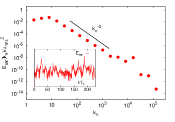
Figure 3: MAIN PANEL: Time-averaged (over the steady state) energy spectrum, normalized by the mean square velocity $u_{\text{rms}}^{2}=\overline{\sum_{n}|u_{n}|^{2}}$, from the simulation of the shell model for active turbulence, Eq. (Three-dimensional active turbulence in microswimmer suspensions: simulations and modelling.). INSET: Total energy, $E_{\text{tot}}(t)=\sum_{n}|u_{n}|^{2}$, vs time (in units of the integral scale characteristic time $T_{L}=(k_{\text{max}}u_{\text{rms}})^{-1}$).

The spectrum decays over a quite wide range of wavenumbers as $E_{\text{sm}}(k_{n})\sim k_{n}^{-3}$ (solid line in Fig. 3), in agreement with the DNS and with an analytical prediction obtained from the shell model (see Supplemental Material).

The PDFs of the velocity variables $u_{n}$, which represent fluctuations on a length scale $\sim k_{n}^{-1}$ ( the shell model counterpart of the velocity increments PDFs in the DNS), provide further insight on the statistical properties of the SabrActive model,

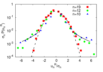
Figure 4: PDFs of the real part of the shell model velocity variables (in units of their root mean square values, $\sigma_{n}$) with three different shell indices, corresponding to length scales within the generalized inertial range ($n=10$ and $n=12$) and down to the microswimmer scale ($n=19$). The dashed line depicts the Gaussian probability density function with zero mean and standard deviation $\sigma=1.5$, whereas the solid lines highlight power law tails of the form $\sim|u_{n}^{R}|^{-\alpha}$, with $\alpha=2.5$.

Fig. 4 displays the normalized PDFs of the real part of the shell velocity variable, $u_{n}^{R}\equiv\operatorname{Re}(u_{n})$ (divided by its root mean square value, $\sigma_{n}$). For the smallest scales, $n=19$ (interpretable as equivalent to that of a microswimmer), the data lie on a Gaussian (dashed line), analogously to what observed in the DNS (see inset of Fig 2). At smaller $n$ (larger scales, falling within the generalized inertial range), the PDFs maintain a Gaussian core, but develop power-law tails at large $u_{n}^{R}$ ($\gtrapprox 4\sigma_{n}$, solid lines). Pinpointing the origin of this discrepancy with the DNS is not obvious and deserves a deeper analysis. A possible explanation dwells in the much longer times covered (roughly a factor $t_{\text{run}}^{\text{(SM)}}/t_{\text{run}}^{\text{(DNS)}}\sim 10^{2}$, once the SM, $t_{\text{run}}^{\text{(SM)}}$, and DNS, $t_{\text{run}}^{\text{(DNS)}}$, runlengths are given in units of the respective integral time scales): intermittency, in fact, is associated with rare events, whose statistical incidence to be appreciated needs, therefore, long observation times. The detection of intermittency signatures in the shell model simulations is intriguing and should motivate further computational studies as well as dedicated experiments.

We have presented a computational and theoretical study aimed at revealing the presence of active turbulence in pusher suspensions in conditions of semi-dilution, namely far from close packing but above the onset of collective motion. We reported that the Eulerian solvent velocity is Lévy-distributed, similarly to previous experimental and theoretical results Rushkin et al. (2010); Zaid et al. (2011). We showed that the energy spectrum develops decays with the power-law $k^{-3}$ over a range of intermediate wavenumbers. It was posited that, given the lack of a Richardson-Kolmogorov energy cascade as in classical turbulence, the excitation of motion at large scales should be ascribed to the coupling between fluid velocity gradients and microswimmer orientation, i.e. to the flow alignment mechanism. Based on this picture and on phenomenological arguments, we developed a reduce order dynamical deterministic model (or shell model) of active turbulence, dubbed SabrActive model. Numerical simulations and theoretical analysis of the model confirmed the $k^{-3}$ scaling of the spectrum.
The introduction of this new model pushes forward the reach of quantitative tests of how actually ”turbulent” is active turbulence, allowing to measure, e.g., Lyapunov exponents, higher order structure functions, multiscale statistics, etc, on ”physically” much longer runs. A flavour of this capability can be grasped in the observation of intermittency in the PDFs of shell model velocity variables. The insight provided will motivate further analysis of the dynamical and statistical properties of the model and the sensitivity of the system response to changes in the control parameters (for instance, the onset of active turbulence at changing the ”activity parameter”), as well as exploring a wider region of the volume-fraction/squirming-parameters space in DNS.
I.P. acknowledges support from Ministerio de Ciencia, Innovación y Universidades MCIU/AEI/FEDER for financial support under grant agreement PID2021-126570NB-100 AEI/FEDER-EU, from Generalitat de Catalunya under Program Icrea Acadèmia and project 2021SGR-673. A.S. acknowledges support from the European Research Council under the European Union Horizon 2020 Framework Programme (No. FP/2014-2020)/ERC Grant Agreement No. 739964 (COPMAT). This work was possible thanks to the access to the MareNostrum Supercomputer at Barcelona Supercomputing Center (BSC) and also through the Partnership for Advanced Computing in Europe (PRACE).

Supplemental Material

.1 SabrActive shell model: the non-linear terms

The hydrodynamics of diluted active suspensions can be described by the following set of equations of motion Aditi Simha and Ramaswamy (2002); Hatwalne et al. (2004); Saintillan and Shelley (2008a, b); Baskaran and Marchetti (2009),

$$\rho(\partial_{t}\mathbf{u}+\mathbf{u}\cdot\nabla)\mathbf{u} =-\nabla p+\eta\nabla^{2}\mathbf{u}+\nabla\cdot\mathbf{\sigma}^{(a)}$$

$$\partial_{t}\mathbf{P}+(\mathbf{u}+w\mathbf{P})\cdot\nabla\mathbf{P} =\mathbf{\Omega}\cdot\mathbf{P}-\Gamma\mathbf{P}+D\nabla^{2}\mathbf{P};$$ (5)

As discussed in the main text, taking the cue from shell models developed for the dynamics of polymer solutions Bird et al. (1987); Benzi et al. (2003); Ray and Vincenzi (2016), we propose a finite-dimensional deterministic model, emulating Eqs. (.1), which consists of a system of coupled ODE’s for the evolution of Fourier amplitudes of fluid velocity and particle orientation fluctuations. The full shell model for Eqs. (.1) reads:

$$\dot{u}_{n} =\frac{i}{3}\Phi^{(\varepsilon)}_{n}(u,u)-\gamma_{u}(k_{n})u_{n}+f^{(a)}_{n}$$

$$\dot{P}_{n} =\frac{i}{3}\Phi^{(\varepsilon)}_{n}(u,P)+\frac{i}{3}w\Phi^{(\varepsilon)}_{n}(P,P)-\frac{i}{3}\Phi^{(\varepsilon)}_{n}(P,u)-\gamma_{P}(k_{n})P_{n}-\Gamma P_{n}.$$ (6)

In this section we provide further details on the non-linear terms corresponding to th generalized Sabra operator $\Phi^{(\varepsilon)}_{n}(u,v)$ L’vov et al. (1998); Benzi et al. (2003), which determines the transfer of energy and/or orientation magnitude across scales. Deciding the direction of transfer of fluctuations is not obvious because in active turbulence the analog of the Richardson picture Frisch (1995), which implies a direct cascade in 3D inertial turbulence, is missing. We need, then, to propose an equivalent phenomenology that goes as follows. First of all, since collective phenomena in active fluids are viscous, we enforce a zero Reynolds number regime and do not account for non-linear momentum transfer, setting $\Phi_{n}^{(\varepsilon)}(u,u)=0\quad\forall n$ in (.1). The velocity of active fluids is governed by a scale-matched balance of active forcing and viscous dissipation Carenza et al. (2020a); Alert et al. (2020); accordingly, the divergence of the active stress $\sigma^{(a)}$ is described by a local-in-scale (or, equivalently, in wavenumber) force in the shell model, $\nabla\cdot\sigma^{(a)}\rightarrow f^{(a)}_{n}=ik_{n}\zeta P_{n}^{2}$. Flow alignment, whereby velocity gradients are coupled to microswimmers’ orientations  Aditi Simha and Ramaswamy (2002); Hernández-Ortiz et al. (2005); Saintillan and Shelley (2007), provides a different mechanism, related to the emergence of collective motion (involving $P$), that excite multiple scales in the fluid, generating turbulence. Consistently, we assume that the rotation term, $P\nabla u$, is responsible for the upwards transfer, and set $\varepsilon=\varepsilon_{b}<\varepsilon_{c}$ in the operator $\Phi^{(\varepsilon)}_{n}(P,u)$ in (.1). Moreover, the advective, $u\nabla P$, and self-advective, $P\nabla P$, terms have mixing properties that tend to disrupt spatial orientational coherence and, therefore, to transfer downwards; we set, then, $\varepsilon=\varepsilon_{f}>\varepsilon_{c}$ in the operators $\Phi^{(\varepsilon)}_{n}(u,P)$ and $\Phi^{(\varepsilon)}_{n}(P,P)$ in (.1). These assumptions have been empirically checked a posteriori and found confirmation in the DNS, as shown in the next section. These mechanisms lead eventually to the SabrActive shell model

$$\dot{u}_{n} =-\gamma_{u}(k_{n})u_{n}+i\zeta k_{n}P_{n}^{2}$$

$$\dot{P}_{n} =\frac{i}{3}\Phi^{(\varepsilon_{f})}_{n}(u,P)+\frac{i}{3}w\Phi^{(\varepsilon_{f})}_{n}(P,P)-\frac{i}{3}\Phi^{(\varepsilon_{b})}_{n}(P,u)-\gamma_{P}(k_{n})P_{n}-\Gamma P_{n}+\delta_{n,n_{B}}|P_{n}|^{-1}P_{n}P_{B}.$$ (7)

.2 Validation of the phenomenological assumptions from the numerics

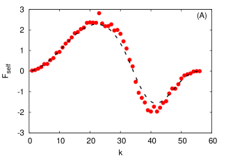
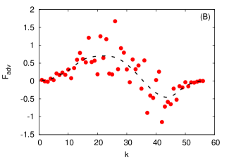
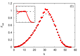
Figure 5: Spectral fluxes, Eq. (11), measured from the numerical simulations (time-averaged over the statistically stationary state): $\mathcal{F}_{\text{self}}$ (A), $\mathcal{F}_{\text{adv}}$ (B) and $\mathcal{F}_{\text{rot}}$ (C); the dashed lines depict a spline interpolation to the data. In the inset of panel (C) the flux per unit area (in spectral space), $k^{-2}\mathcal{F}_{\text{rot}}$ is shown, highlighting the presence of constant flux range of scales.

We have seen in the previous section how the development of a shell model relies crucially on the knowledge of the transfer of dynamical fluctuations of a field across scales. Lacking a Richardson cascade, we had to conjecture the direction of fluxes in spectral space of non-linear terms involving the orientation and velocity field on the basis of phenomenological arguments. Here, we want to justify these conjectures, benchmarking them against direct numerical simulations. Since our numerical method couples a Lagrangian dynamics for bacteria with a Eulerian description of the fluid, though, first we need a procedure that maps the particle positions and orientations to the field $\mathbf{P}$. To this aim we divide ideally the computational box in $(L/\Delta)^{3}$ subdomains $\mathcal{I}_{\Delta}^{(m)}=\{\mathbf{x}\in L^{3}:|x_{i}-X^{(m)}_{i}|<\Delta/2,\,i=1,2,3\}$ and introduce the following representation of $\mathbf{P}$

$$\mathbf{P}_{\Delta}(\mathbf{X}^{(m)},t)=\frac{1}{N_{\Delta}^{(m)}(t)}\sum_{i}^{N_{\Delta}^{(m)}(t)}\hat{e}_{i}(t),$$ (8)

on the lattice defined by the set of points $\mathbf{X}_{m}=\Delta/2+\mathbf{m}\Delta$, with $\mathbf{m}=(m_{x},m_{y},m_{z})$ a vector of integers ranging from $0$ to $L/\Delta-1$. The sum in (8) runs over the $N_{\Delta}^{(m)}$ particles contained in $\mathcal{I}_{\Delta}^{(m)}$ at time $t$. Analogously we construct a velocity field that lives on the coarse lattice as:

$$\mathbf{u}_{\Delta}(\mathbf{X}_{m},t)=\frac{1}{\Delta^{3}}\sum_{\mathbf{x}\in\mathcal{I}_{\Delta}^{(m)}}\mathbf{u}(\mathbf{x},t).$$ (9)

At this point by projecting the second of Eqs. (.1), with $\mathbf{u}$ and $\mathbf{P}$ replaced by $\mathbf{u}_{\Delta}$ and $\mathbf{P}_{\Delta}$, onto the Fourier mode $\mathbf{k}$, multiplying both sides by $\tilde{\mathbf{P}}_{\Delta}^{\ast}$ (the complex conjugate of the Fourier transform of $\mathbf{P}_{\Delta}$), averaging over shells of radius $k$ and summing with the complex conjugate equation, we get:

$$(\partial_{t}+\Gamma+Dk^{2})\mathcal{P}_{\Delta}=\mathcal{F}_{\text{adv}}+\mathcal{F}_{\text{self}}+\mathcal{F}_{\text{rot}},$$ (10)

where $\mathcal{P}(k,t)=\langle|\tilde{\mathbf{P}}_{\Delta}|^{2}\rangle$. The terms on the right hand side read as follows:

$$\mathcal{F}_{\text{adv}}(k,t) =-\langle\left(\tilde{\mathbf{P}}_{\Delta}^{\ast}(\mathbf{k},t)\cdot\mathbf{J}_{\text{uP}}(\mathbf{k},t)\right)\rangle+\mbox{c.c.}$$ (11)

$$\mathcal{F}_{\text{self}}(k,t) =-\langle\left(\tilde{\mathbf{P}}_{\Delta}^{\ast}(\mathbf{k},t)\cdot\mathbf{J}_{\text{PP}}(\mathbf{k},t)\right)\rangle+\mbox{c.c.}$$

$$\mathcal{F}_{\text{rot}}(k,t) =\langle\left(\tilde{\mathbf{P}}_{\Delta}^{\ast}(\mathbf{k},t)\cdot\mathbf{\mathcal{R}}(\mathbf{k},t)\right)\rangle+\mbox{c.c.}$$

where $\mathbf{J}_{\text{uP}}(\mathbf{k},t)$, $\mathbf{J}_{\text{PP}}(\mathbf{k},t)$ and $\mathbf{\mathcal{R}}(\mathbf{k},t)$ are the Fourier transforms of the non-linear terms of the orientation field equation, namely $\mathbf{u}_{\Delta}\cdot\nabla\mathbf{P}_{\Delta}$, $w\mathbf{P}_{\Delta}\cdot\mathbf{P}_{\Delta}$ and $\mathbf{\Omega}_{\Delta}\cdot\mathbf{P}_{\Delta}$, respectively, and ”c.c.” stands for the complex conjugate terms. Eqs. (11) are fluxes across $k$-shells in spectral space and whether a direct or inverse cascade of magnitude of orientation, depending on their sign, takes place. We measured them in then numerical simulations and the results, averaged in time over the statistically stationary state are plotted in Fig. 5. Although the coarse-graining procedure reduced the range of accessible scales, a clear qualitative difference appears: while $\mathcal{F}_{\text{adv}}$ and $\mathcal{F}_{\text{self}}$ (top and middle panels) are negative at intermediate and large wavenumbers, signalling that they transfer orientation fluctuations towards small scales (i.e. they tend to disrupt coherence), the rotational spectral flux $\mathcal{F}_{\text{rot}}$ (bottom panel) is positive (and in magnitude larger than the previous two), therefore confirming our phenomenological conjecture that it is the term responsible for the upward cascade that eventually pumps energy into the large scales.

.3 Energy spectrum from the shell model

We show here how it is possible to derive the power law decay of the energy spectrum, $E(k)\sim k^{-3}$, from the shell model. The evolution of the orientation magnitude, $|P_{n}|^{2}$, is obtained multiplying the second of Eqs. (.1) by $P_{n}^{\ast}$ and the complex conjugate by $P_{n}$ and summing the two, and reads

$$\partial_{t}|P_{n}|^{2}\approx P_{n}^{\ast}\Phi^{(\varepsilon_{b})}_{n}(P,u)+P_{n}(\Phi^{(\varepsilon_{b})}_{n}(P,u))^{\ast}-\Gamma|P_{n}|^{2}-\gamma(k_{n})|P_{n}|^{2},$$ (12)

where the advective and self-advecting terms are neglected, consistent with the DNS results, see Fig. 5. Assuming statistical stationarity and focusing on intermediate $k_{n}$, where the flux dominates over dissipation (i.e. we look at the generalized inertial range), we see immediately that, dimensionally, $kuP^{2}\sim\mbox{cte}$ whence,

$$P\sim k^{-1/2}u^{-1/2}.$$ (13)

From the first of Eqs. (.1) we get analogously that $k^{2}u^{2}\sim kuP^{2}$, whence

$$u\sim k^{-1}P^{2}.$$ (14)

Plugging Eq. (13) into Eq. (14) yields $u_{n}\sim k_{n}^{-1}$, therefore the energy spectrum, $k_{n}^{-1}|u_{n}|^{2}$, should indeed behave as

$$E_{\text{sm}}(k_{n})\sim k_{n}^{-3}.$$ (15)

References

- Vicsek and Zafeiris (2012) T. Vicsek and A. Zafeiris, Phys. Rep. 517, 71 (2012).
- Kearns (2010) D. Kearns, Nat. Rev. Microbiol. 8, 634 (2010).
- Darnton et al. (2010) N. Darnton, L. Turner, S. Rojevsky, and H. Berg, Biophys. J. 98, 2082 (2010).
- Koch and Subramanian (2011) D. Koch and G. Subramanian, Annu. Rev. Fluid Mech. 43, 637 (2011).
- Ballerini et al. (2008) M. Ballerini, N. Cabibbo, R. Candelier, A. Cavagna, E. Cisbani, I. Giardina, V. Lecomte, A. Orlandi, G. Parisi, A. Procaccini, M. Viale, and V. Zdravkovic, Proc. Natl. Acad. Sci. USA 105, 1232 (2008).
- Herbert-Read et al. (2011) J. Herbert-Read, A. Perna, R. Mann, T. Schaerf, D. Sumpter, and A. Ward, Proc. Natl. Acad. Sci. USA 108, 18726 (2011).
- Dombrowski et al. (2004) C. Dombrowski, L. Cisneros, S. Chatkaew, R. Goldstein, and J. Kessler, Phys. Rev. Lett. 93, 098103 (2004).
- Wolgemuth (2008) C. Wolgemuth, Biophys. J. 95, 1564 (2008).
- Pedley and Kessler (1992) T. Pedley and J. Kessler, Annu. Rev. Fluid Mech. 23, 313 (1992).
- Alert and Casademunt (2020) R. Alert and J.-F. Casademunt, J. Joanny, Annu. Rev. Condens. Matter Phys. 13, 143 (2020).
- Vallis (1999) G. Vallis, Lecture Notes on ”Geostrophys turbulence: the macroturbulence of the atmosphere and ocean” (1999).
- Ishikawa et al. (2011) T. Ishikawa, N. Yoshida, H. Uedo, M. Wiedemann, Y. Imai, and T. Yamaguchi, Phys. Rev. Lett. 107, 028102 (2011).
- Wensink et al. (2012) H. Wensink, J. Dunkel, S. Heidenreich, K. Drescher, R. Goldstein, H. Löwen, and J. Yeomans, Proc. Natl. Acad. Sci. USA 109, 14308 (2012).
- Kokot et al. (2015) G. Kokot, S. Das, R. Winkler, G. Gomppper, I. Aranson, and A. Snezhko, Proc. Natl. Acad. Sci. USA 112, 15048 (2015).
- Doostmohammadi et al. (2017) A. Doostmohammadi, T. Shendruk, K. Thijssen, and J. Yeomans, Nat. Commun. 8, 15326 (2017).
- Martínez-Prat et al. (2019) B. Martínez-Prat, J. Ignés-Mullol, J. Casademunt, and F. Sagués, Nature Physics 15, 362 (2019).
- Bourgoin et al. (2020) M. Bourgoin, R. Kervil, C. Cottin-Bizonne, R. Raynal, R. Volk, and C. Ybert, Phys. Rev. X 10, 021065 (2020).
- Bratanov et al. (2015) V. Bratanov, F. Jenko, and E. Frey, Proc. Natl. Acad. Sci. USA 112, 15048 (2015).
- Frisch (1995) U. Frisch, Turbulence (Cambridge University Press, 1995).
- Słomka and Dunkel (2017) L. Słomka and J. Dunkel, Proc. Natl. Acad. Sci. USA 114, 2119 (2017).
- Linkmann et al. (2019) M. Linkmann, G. Boffetta, M. Marchetti, and B. Eckhardt, Phys. Rev. Lett. 122, 214503 (2019).
- Carenza et al. (2020a) L. Carenza, L. Biferale, and G. Gonnella, Phys. Rev. Fluid 5, 011302(R) (2020a).
- Carenza et al. (2020b) L. Carenza, L. Biferale, and G. Gonnella, Europhys. Lett. 132, 44003 (2020b).
- Alert et al. (2020) R. Alert, J.-F. Joanny, and J. Casademunt, Nat. Phys. 16, 682 (2020).
- Rorai et al. (2022) C. Rorai, F. Toschi, and I. Pagonabarraga, Phys. Rev. Lett. 129, 218001 (2022).
- Kruse et al. (2004) K. Kruse, J. Joanny, F. Jülicher, J. Prost, and K. Sekimoto, Phys. Rev. Lett. 92, 078101 (2004).
- Giomi et al. (2008) L. Giomi, M. Marchetti, and T. Liverpool, Phys. Rev. Lett. 101, 198101 (2008).
- Edwards and Yeomans (2008) S. Edwards and J. Yeomans, Europhys. Lett. 85, 18008 (2008).
- Tjhung et al. (2011) E. Tjhung, M. Cates, and D. Marenduzzo, Soft Matter 7, 7453 (2011).
- Słomka and Dunkel (2015) L. Słomka and J. Dunkel, Eur. Phys. J. Spec. Top. 224, 1349 (2015).
- Stenhammar et al. (2017) J. Stenhammar, C. Nardini, , R. Nash, D. Marenduzzo, and A. Morozov, Phys. Rev. Lett. 119, 028005 (2017).
- Bárdfalvy et al. (2019) D. Bárdfalvy, H. Nordanger, C. Nardini, A. Morozov, and J. Stenhammar, Soft Matter 15, 7747 (2019).
- Škultéty et al. (2020) V. Škultéty, C. Nardini, J. Stenhammar, D. Marenduzzo, and A. Morozov, Phys. Rev. X 10, 031059 (2020).
- Wu and Libchaber (2000) X.-L. Wu and A. Libchaber, Phys. Rev. Lett. 84, 3017 (2000).
- Hernández-Ortiz et al. (2005) J. Hernández-Ortiz, C. Stoltz, and M. Graham, Phys. Rev. Lett. 95, 204501 (2005).
- Leptos et al. (2009) K. Leptos, J. Guasto, J. Gollub, A. Pesci, and R. Goldstein, Phys. Rev. Lett. 103, 198103 (2009).
- Saintillan and Shelley (2012) D. Saintillan and M. Shelley, J. R. Soc. Interface 9, 571 (2012).
- Liu et al. (2021) Z. Liu, W. Zeng, X. Ma, and X. Cheng, Soft Matter 17, 10806 (2021).
- Biferale (2004) L. Biferale, Annu. Rev. Fluid Mech. 35, 441 (2004).
- Succi (2018) S. Succi, The lattice Boltzmann equation for complex state of flowing matter (Oxford University Press, 2018).
- Wolf-Gladow (2000) D. Wolf-Gladow, Lattice–gas cellular automata and lattice Boltzmann models. An introduction (Springer, 2000).
- Desplat et al. (2001) J.-C. Desplat, I. Pagonabarraga, and P. Bladon, Comp. Phys. Commun. 134, 273 (2001).
- Ladd (1994) A. Ladd, J. Fluid Mech. 271, 285 (1994).
- Nguyen and Ladd (2002) N. Nguyen and A. Ladd, Phys. Rev. E 66, 046708 (2002).
- Aidun and Clausen (2010) C. Aidun and J. Clausen, Annu. Rev. Fluid Mech. 42, 439 (2010).
- Blake (1971) J. Blake, J. Fluid Mech. 46, 199 (1971).
- Ishikawa et al. (2006) T. Ishikawa, M. Simmonds, and T. Pedley, J. Fluid Mech. 568, 119 (2006).
- Matas Navarro and Pagonabarraga (2010) R. Matas Navarro and I. Pagonabarraga, Eur. Phys. J. E 33, 27 (2010).
- Alarcón and Pagonabarraga (2013) F. Alarcón and I. Pagonabarraga, J. Mol. Liq. 185, 56 (2013).
- Alarcón et al. (2017) F. Alarcón, C. Valeriani, and I. Pagonabarraga, Soft Matter 13, 814 (2017).
- Scagliarini and Pagonabarraga (2022) A. Scagliarini and I. Pagonabarraga, Soft Matter 18, 2407 (2022).
- Zaid et al. (2011) I. Zaid, J. Dunkel, and J. Yeomans, J. R. Soc. Interface 8, 1314 (2011).
- Rushkin et al. (2010) I. Rushkin, V. Kantsler, and R. Goldstein, Phys. Rev. Lett. 105, 188101 (2010).
- Gledzer (1973) E. Gledzer, Sov. Phys. Dokl. 18, 216 (1973).
- Desnyansky and Novikov (1974) V. Desnyansky and E. Novikov, Izv. Akad. Nauk SSSR Fiz. Atmos. Okeana 10, 127 (1974).
- Bohr et al. (1998) T. Bohr, M. Jensen, G. Paladin, and A. Vulpiani, Dynamical systems approach to turbulence (Cambridge University Press, 1998).
- Benzi et al. (2003) R. Benzi, E. De Angelis, R. Govindarajan, and I. Procaccia, Phys. Rev. E 68, 016308 (2003).
- Benzi et al. (2004) R. Benzi, N. Horesh, and I. Procaccia, Europhys. Lett. 68, 310 (2004).
- Ray and Vincenzi (2016) S. Ray and D. Vincenzi, Europhys. Lett. 144, 44001 (2016).
- Note (1) The system for the velocity variables is coupled, in this case, to a set of equations for analogous polymer variables, interpreted as spectral amplitudes of an auxiliary vector field whose dyadic product is the polymer conformation tensor Benzi et al. (2003).
- Aditi Simha and Ramaswamy (2002) R. Aditi Simha and S. Ramaswamy, Phys. Rev. Lett. 89, 058101 (2002).
- Hatwalne et al. (2004) Y. Hatwalne, S. Ramaswamy, M. Rao, and R. Aditi Simha, Phys. Rev. Lett. 92, 118101 (2004).
- Saintillan and Shelley (2008a) D. Saintillan and M. Shelley, Phys. Rev. Lett. 100, 178103 (2008a).
- Saintillan and Shelley (2008b) D. Saintillan and M. Shelley, Phys. Fluids 20, 123304 (2008b).
- Baskaran and Marchetti (2009) A. Baskaran and M. Marchetti, Proc. Natl. Acad. Sci. USA 106, 15567 (2009).
- Bird et al. (1987) R. Bird, R. Armstrong, and O. Hassager, Dynamics of Polymeric Liquids (John Wiley and sons, 1987).
- L’vov et al. (1998) V. L’vov, E. Podivilov, A. Pomyalov, I. Procaccia, and D. Vandembroucq, Phys. Rev. E 58, 1811 (1998).
- Gilbert et al. (2002) T. Gilbert, V. L’vov, A. Pomyalov, and I. Procaccia, Phys. Rev. Lett. 89, 074501 (2002).
- Pisarenko et al. (1993) D. Pisarenko, L. Biferale, D. Courvoisier, U. Frisch, and M. Vergassola, Phys. Fluids 5, 2533 (1993).
- Saintillan and Shelley (2007) D. Saintillan and M. Shelley, Phys. Rev. Lett. 99, 058102 (2007).