Dr. KID: Direct Remeshing and K-set Isometric Decomposition for Scalable Physicalization of Organic Shapes

Abstract

Dr. KID is an algorithm that uses isometric decomposition for the physicalization of potato-shaped organic models in a puzzle fashion. The algorithm begins with creating a simple, regular triangular surface mesh of organic shapes, followed by iterative K-means clustering and remeshing. For clustering, we need similarity between triangles (segments) which is defined as a distance function. The distance function maps each triangle’s shape to a single point in the virtual 3D space. Thus, the distance between the triangles indicates their degree of dissimilarity. K-means clustering uses this distance and sorts segments into k classes. After this, remeshing is applied to minimize the distance between triangles within the same cluster by making their shapes identical. Clustering and remeshing are repeated until the distance between triangles in the same cluster reaches an acceptable threshold. We adopt a curvature-aware strategy to determine the surface thickness and finalize puzzle pieces for 3D printing. Identical hinges and holes are created for assembling the puzzle components. For smoother outcomes, we use triangle subdivision along with curvature-aware clustering, generating curved triangular patches for 3D printing. Our algorithm was evaluated using various models, and the 3D-printed results were analyzed. Findings indicate that our algorithm performs reliably on target organic shapes with minimal loss of input geometry.

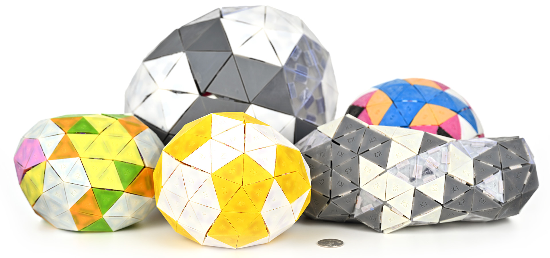
Figure 1: The physicalization of potato-shaped biological structures with $k$ types of triangles. Back row: SARS-CoV-2 virion membrane (left) with $k=2$, SARS-CoV-2 virion membrane with smooth triangle patches (right), using $k=6$, and front row: cell nuclei membrane (left), using $k=5$, SARS-CoV-2 virion membrane (center), using $k=2$, mitochondria outer membrane (right), using $k=6$.

Keywords Physicalization $\cdot$ Physical visualization $\cdot$ 3D printing $\cdot$ Isometric decomposition $\cdot$ Direct remeshing $\cdot$ Biological structures $\cdot$ Intracellular compartments.

1 Introduction

Physical models are powerful tools for understanding and comprehending complex objects and systems. They provide a simplified representation of an object’s shape, structure, function, and inner composition, making it easier for individuals to grasp the intricacies of the object (Bailey et al., 1998; Casas and Estop, 2015). Physical visualization bridges the gap between digital data and its physical composition (Bader et al., 2018). This is especially true for objects that are too large to take in all details at once, too small to depict their inner structure, or too complex to fully understand the interconnectedness of their parts and how they work together. Physical visualizations are often implemented as 3D puzzles.

3D puzzles, in particular, offer an engaging and challenging form of entertainment that can help improve spatial reasoning and problem-solving skills (Verdine et al., 2014; Nicolaidou et al., 2021; Lin et al., 2022). They illustrate the real-world object’s inner structure in a way that can be easily understood, allowing individuals to gain a deeper understanding of the object and its workings. In addition to being a source of entertainment, 3D puzzles can also be used in education as a tool to teach how things are built and how they function (Casas and Estop, 2015). They can also be used in outreach to attract people’s attention and ignite an interest in a specific topic. For such use cases, puzzles are actually data physicalization (Moere, 2008; Zhao and Moere, 2008; Jansen et al., 2013, 2015; Dragicevic et al., 2020; Djavaherpour et al., 2021) intended to familiarize the users with the data they are based on.

A world of mesoscale biological models is an appropriate domain for such puzzles representing the intricate and detailed structures of living organisms at the cellular and subcellular levels. Mesoscale biological structures are typically very complex and are built of many small building blocks. Assembling such puzzles allows individuals to gain a deeper understanding and appreciation of biological systems’ complex and dynamic nature. Furthermore, the physical nature of these puzzles provides for a hands-on learning experience, helping to make the information more memorable and engaging (Echavarria et al., 2020), which is beneficial in educational settings as a tool for teaching anatomy, physiology, and biology (Hidayat et al., 2019). They can also be beneficial for research purposes, for example, to help scientists study the structure of proteins or viruses (Nguyen et al., 2021).

For a 3D puzzle to be suitable for injection molding production, it is important to minimize the number of different parts in the design because the cost of producing the molds for injection molding is directly related to the number of elements in the puzzle and is the costliest part in the pipeline. It is also important to keep in mind that the puzzle’s design should be optimized for the injection molding process to ensure that it can be produced efficiently and with minimal defects. This could include simplifying the puzzle’s geometry, avoiding deep undercuts and sharp corners, and ensuring that the puzzle’s parts can be easily removed from the mold.

To enable scalable generation of 3D puzzles representing biological systems such as viruses, organelles, or cells, it is meaningful to use the molding process for generating all the building blocks. Often, these potato-shaped structures are surrounded by a membrane formed by a lipid bilayer. The membrane is richly decorated with macromolecular protein complexes, which are also forming the lumen of the biological system. Additionally, there are numerous fibrous structures, such as microtubules, actin fibers, and genetic macromolecules, that contribute to the internal ultrastructure of the biological system. In a viral particle, for example, a few unique protein structures form the mature virus, which are instantiated in the virus numerous times. This is ideal for the molding process for the purposes of data physicalization. One of the main problems is how to represent the lipid bilayer, which is the basis of the shape of the biological system. In the case of an ideal sphere, the surface can be assembled from identical spherical triangular patches. However, real biological structures are never perfect spheres. Their shapes are more similar to a potato, cucumber, or bean. Tesselating the surface of such 3D shapes results in a set of unique triangles, i.e., every triangle is different. Such tessellation is prohibitive in the context of scalable 3D puzzle generation, as the number of unique pieces is too high for viable puzzle production. Therefore, we need a tessellation that approximates the shape well and, at the same time, is made out of very few distinct classes of triangle patches. This problem constitutes the intellectual challenge of this paper.

We present a puzzle-generation system called Dr. KID , which generates a surface mesh of biological structure and decomposes it into reconfigurable puzzle components (segments). The segments can be either planar triangles (planar patches) or curved triangular patches (curved patches). We focus on the isometric decomposition of the surface, where we take the surface mesh of the model and decompose it into a set of $k$ isometric segments (identical components). Following the surface thickening stage, we create connector structures for assembling and disassembling the puzzle segments. We use unique hinge joint connector parts for connecting the segments. For these connector hinge joints, we created identical holes on each side of all the triangle segments. Dr. KID solves a geometric problem and provides a real-world prototype for scientific outreach using data physicalization. It is scoped for depicting a micron-sized biological system but can be used for creating 3D puzzles of any potato-like shapes.

The technical contributions of the proposed work are summarized below:

• A new distance measure for K-means isometric decomposition of the surface into triangular patches.

• Surface remeshing with novel cluster-aware local operators for within-cluster distances minimization and thus improving isometries of within-cluster patches.

• A novel automatic process of curvature-aware surface thickening of triangular patches and connector-placement design.

• Application of isometric decomposition for data physicalization of potato-shaped objects showcased on biological structures.

2 Related Work

This section presents related work from various domains, including scalable physicalization, Isometric decomposition, 3D puzzles, and surface remeshing.

Isometric decomposition of a surface is a challenging task that can generate identical puzzle parts for reconfigurable 3D models. In addition to 3D puzzles, isometric decomposition plays an important role in various fields of computational design, including architectural geometry, fabrication, modeling, surface reconstruction, and more. One of its main uses is generating isometric segments of the input surface. This complex geometric problem enhances reusability, reducing both complexity and costs (Jiang et al., 2021; Zimmer and Kobbelt, 2014; Huard et al., 2015; Liu et al., 2021). Isometric decomposition has applications in tiling (Fu et al., 2010), modeling, and fabrication (Liu et al., 2021). Depending on the surface mesh and application, surfaces can be decomposed into triangles (Liu et al., 2021; Singh and Schaefer, 2010), quads (Fu et al., 2010), or other polygonal segments.

To the best of our knowledge, the first attempt at the isometric decomposition of curved surfaces was conducted by Singh and Schaefer (2010). They employed a set of template triangles called canonical triangles and remeshed the model to make each triangle in the mesh identical to one of those. Their method (Singh and Schaefer, 2010) does not allow topology change and needs higher numbers of triangles to preserve the desired shape. Furthermore, they start with a single cluster and add more clusters later. They used global optimization instead of direct remeshing. Although their method accommodates curved surfaces, the canonical triangles remain planar, and there is no mechanism to address surface thickness. Planar penalization (Huard et al., 2015) is another attempt to reduce complexity by creating repetitive patterns. The work by Fu et al. (2010) on K-set tileable surfaces presents a similar approach for quad meshes, generating similar quads. This approach offers a fascinating solution for minimizing the number of fabricated components into a given number of $k$ quads. However, using quad meshes can drastically alter the original shape when minimizing the value of $k$. While the authors mention that this idea can be extended for puzzle-like reassembleable applications, no such extension currently exists.

Liu et al. (2021) proposed a method for modeling and fabrication with a minimal number of classes of equivalent triangles. This method is the most relevant for our current work. However, this method uses existing template triangles, which are meant for large fabrication models and therefore do not require addressing their thickness. The connection among the triangles is established via holes and nylon cable. Moreover, the triangles are planar, and the curvature is created at connection points among the triangles. Therefore, the smoothness of the models is not realistic.

In summary, the literature review yields several methods for isometric decomposition. However, due to their limitations, these methods are not practical for puzzles and physicalization. For example, all these methods anticipate having existing templates rather than supporting a dynamic number of pieces. The structures generated with them also rely on external support to keep the individual surfaces in place. Furthermore, the existing methods have no mechanisms for surface thickness, which is essential for the independent assembly of the models or surface smoothness. The k-set tileable quads method by Fu et al. (2010) drastically changes the input model if decreasing the number of segments. Moreover, there is less attenuation toward biological models. Unlike CAD models or general architectural geometry, biological models are more challenging.

Isometric patterns are highly encouraged in architectural geometry and civil engineering. In this regard, Jiang et al. (2021) used isometric bending of surfaces via a small set of molds to create manufacturable tiles, which addresses the problem of representing free forms. They only used constant Gaussian curvature for this paneling. Developability of a B-spline surface (Gavriil et al., 2019) improves the paneling task and can reduce manufacturing costs significantly. This paneling method (Gavriil et al., 2019) locally approximates the 1-dimensional Gauss image with a circle. The method gives smoother results with higher efficiency. However, it is limited to the grid-like panel arrangement.

Zometool is a mathematical and molecular modeling kit, which is a popular visualization and physicalization tool with a specific focus on repetitive patterns such as molecular structures, crystal lattices, and mathematical constructs. Further research (Zimmer and Kobbelt, 2014; Zimmer et al., 2014) extended the scope of Zometool toward free-form, disk-topology surfaces. The studies (Zimmer and Kobbelt, 2014; Zimmer et al., 2014) provide an insight into utilizing Zometool for architectural applications. Adopting the advancing front strategy, they start from a single vertex and grow forward for the physicalization of the model. They use hybrid meshes (mixed with quads and triangles) for surface representation. They use nine different types of edges. Users, however, cannot select the number of classes. Therefore, there is no option to minimize the number of used polygon classes.

3D puzzles captivate the imagination with their wide-ranging and intricate designs. They encompass an array of types, such as the essential 2-manifold jigsaw puzzles that form the surfaces of 3D objects, as highlighted by Coffin (2006). Polyomino puzzles, presented by Lo et al. (2009), reminiscent of intricate Tetris-like shapes, come together to create elaborate 3D objects. Burr puzzles delight with their interlocking pieces that, when assembled, reveal complete 3D models, as presented by Xin et al. (2011). The enchanting world of recursively interlocking puzzles, presented by Song et al. (2012), takes the complexity of burr puzzles to a higher level. Dissection puzzles offer a transformative experience, as they can be reassembled into various forms as presented by Séquin (2012). Twisty puzzles invite engagement through their assembly or disassembly via twisting motions, as shown by Sun and Zheng (2015). Elber and Kim (2022) present some recent improvements, which address the 3D jigsaw puzzles over 2-manifolds, while Tang et al. (2019) present a novel approach to the computational design of 3D dissection puzzles.

Fabricated 3D puzzles created based on scientific data exemplify data physicalization, transforming abstract information into tangible objects (de Freitas et al., 2022). Tangible data visualization facilitates a more intuitive, engaging, and immersive exploration of complex data structures (Eslambolchilar et al., 2023; Djavaherpour et al., 2021). As users interact with the printed pieces and strive to solve the puzzles, they actively decipher the encoded data, enhancing their cognitive understanding and promoting deeper insights. Consequently, 3D printed puzzles, as a manifestation of data physicalization, offer an innovative and accessible means of visualizing, analyzing, and comprehending information, allowing users to connect with the data on a visceral level, transcending the limitations of traditional, screen-based representations.

The fabrication of 3D puzzles varies greatly depending on the puzzle type. For different puzzle types, multiple factors must be considered, such as printing 3D objects that exceed the printer’s working volume and can later be assembled using custom connectors (Luo et al., 2012; Yao et al., 2015), need to be optimally packed (Chen et al., 2015), or designed as interlocking parts (Song et al., 2015). Some approaches also approximate 3D models using multiple planes, simplifying the fabrication process to two dimensions (Chen et al., 2013), and utilizing unique fabrication methods for the base structure and detailed sections, which can then be merged into one piece (Song et al., 2016). Although cost optimization is most significant in large-scale applications like architectural design (Eigensatz et al., 2010), it offers considerable savings by incorporating 3D printing into the injection molding process chain (Tosello et al., 2019).

Mesh processing has always been an effective way to represent surfaces (Lorensen and Cline, 1987), allowing a variety of surface analyses. They can provide a base for accurate surface decomposition. Surface remeshing (Khan et al., 2022; Alliez et al., 2008) alters the meshes for their quality improvement and/or some other remeshing objectives. Remeshing algorithms are either based on global optimization or use selected local operators. cvt (Lloyd, 1982; Liu et al., 2009) has been widely used for surface remeshing (Khan et al., 2022). It is an improved type of Voronoi diagram, which relocates each seed to the mass center of its Voronoi cell. Typically, this relocation is achieved by minimizing the specific energy function.

Typically, isometric decomposition algorithms have two main tasks, pattern matching to find the similarity among the patches and remeshing to make the patches similar. Pattern matching quantifies the degree of similarity among the patches, whereas remeshing alters their shapes to make them identical to other shapes in the class. Mesh representation also provides opportunities for surface smoothing by triangle subdivision (Loop, 1987). We refer the readers to two comprehensive survey articles on surface remeshing (Khan et al., 2022; Alliez et al., 2008).

3 K-set Isometric Decomposition

The domain of our algorithm is a family of biological structures having a potato-like shape (e.g., mitochondria, lysosome, endosomes, cellular nuclei, virus particles etc.). The goal is to create a cost-effective and appealing physicalization of these shapes. To achieve this goal, we address two challenges: (1) including isometric decomposition with geometric fidelity and (2) curvature-aware modeling of decomposed parts as assemblable parts. The problem is formally stated as follows:

Problem statement:

Our goal is to decompose the surface mesh $M_{i}$ of these structures into a given number of $k$ classes of mesh segments $C=\{c_{1},c_{2},c_{3},\ldots,c_{k}\}$. Each class $c_{i}$ contains a finite number of mesh segments $P=\{p_{i}\}_{i=1}^{|c_{i}|}$ satisfying the following requirement conditions:

• Similarity and distinctions: Any two patches belonging to the same class should be identical to each other and different from patches from other classes. Mathematically, if $p_{i}\in c_{i}$ and $p_{j}\in c_{i}$, then both $p_{i}$ and $p_{j}$ must be identical and distinct otherwise.

• Planar vs. curved segments: Depending on the user’s choice, the patches can be planar (triangular patches) or curved mesh segments (curved patches).

• Geometric fidelity and approximation: The segmented mesh (collection of all patches) should preserve the input shape with an acceptable approximation error.

• Reconfigurable objects: The patches are linked with identical connectors and holes, yielding a set of reconfigurable 3D objects (to be manufactured for the 3D puzzle).

• Patch thickness: Such reconfigurable patches require thickness which is, in our case, provided by the user.

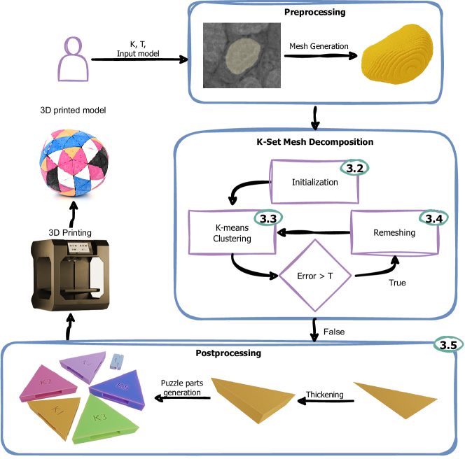
Figure 2: The overview of the presented method illustrating inputs and outputs of the individual steps.

3.1 Method Overview

The method overview is presented in Figure 2 and in more detail by algorithm 1, which presents a pseudocode for the overall physicalization, starting with the 3D shape and ending with the puzzle pieces. The algorithm takes input mesh ($M_{i}$) generated from the input 3D structure, error threshold (T), which represents the acceptable tolerance during remeshing, and the value of $k$ representing the number of classes. The threshold (T) is the maximum permissible error for k-set isometric decomposition. It provides a convergence point (stopping point) to our iterative algorithm. The algorithm starts with mesh generation and initialization (subsection 3.2). The overall idea is to remesh $M_{i}$ and get a final mesh $M_{f}$ satisfying the aforementioned conditions. For clustering, we use a distance measure that maps the similarity among triangles into square Euclidean distances in a 3D space. For K-set isometric triangulation, we minimize the distance defined by Equation 1 by iteratively executing the two consecutive steps: (1) K-means clustering (subsection 3.3) and (2) remeshing (subsection 3.4). Clustering, remeshing, and updating each triangle’s position in our 3D space are repeated until the algorithm converges. After this, the triangles are processed for connecting structures consisting of a hinge joint (connector) and corresponding holes in individual parts (holes). We present an automatic module for making curvature-aware thickness and connectors and holes.

The default classification is for planar triangular patches. However, we also support smoother curved triangular patches by applying the Loop subdivision (Loop, 1987), which gives us a smoother surface (see subsection 3.6). Again, we apply patch-wise classification with a higher value of $k$ using K-means with curvature information to get a final classification of the curved patches.

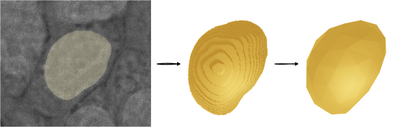
Figure 3: Converting segmented volumetric data (left) to mesh representation using Marching Cubes (middle) and mesh refinement using cvt (right).

Data: $M_{i},T,k,3DShape$

Result: $M_{f}$, k types identical thickened triangles and connectors

1:  $M_{i}\leftarrow\mathrm{SurfaceMesh}(3DShape)$

2:  $M_{s}\leftarrow\mathrm{Init}(M_{i})$

3:  $M_{f}\leftarrow\mathrm{Init}(M_{s})$

4:  $Virtual3Dspcae\leftarrow\mathrm{CalculatePositionin3Dspace}(M_{f})$

5:  $Convergence\leftarrow False$, $Itr\leftarrow 1$

6:  while $(!Convergence)$ do

7:     $\left[Labels,WithinClusterDistances\right]\leftarrow\mathrm{Clustering}(M_{f},k,T)$ // Calling algorithm 2

8:     $M_{f}\leftarrow\mathrm{UpdateClusteringLabels}(Labels,M_{f})$

9:     if $(T\geq\max(WithinClusterDistances))$ then

10:        $Convergence\leftarrow True$ // (see Equation 4 for convergence point)

11:     else

12:        $M_{f}\leftarrow Remeshing(M_{s},k,T,Itr++)$ // Calling algorithm 3

13:        $M_{f}\leftarrow\mathrm{UpdatePositionin3Dspace}(M_{f})$

14:     end if

15:  end while

16:  $VNormals\leftarrow\mathrm{VerticesNormals}(M_{f})$ // for surface thickness.

17:  $\mathrm{GenerateThickenedTriangles}(M_{f})$

18:  Make connector-placement and Hinges.

19:  $END$

Algorithm 1 K-Set Isometric Decomposition

3.2 Mesh Generation and Initialization

For input, we take segmented volumetric data of biological structures such as mitochondria, viral virions, intracellular compartments etc. The segmented structures are converted from voxelized to mesh representation (see Figure 3). We use the Marching cubes algorithm (Lorensen and Cline, 1987) for generating our first raw mesh $(M_{i})$ from the 3D structure. However, this raw mesh has several defects, including self-intersections, higher complexity, and redundant elements. Therefore, prior to actual classification and remeshing, careful refinement is required. We refine $M_{i}$ in initialization step using cvt (Lloyd, 1982; Liu et al., 2009). The initialization step not only improves mesh quality but also simplifies the mesh by setting the number of seeds in cvt. This refined and simplified mesh is denoted by $M_{s}$ throughout this paper. More specifically, the raw mesh is remeshed with two different implementations of the cvt, including 5 iterations of the Lloyd algorithm (Lloyd, 1982) followed by 30 iterations of the quasi-Newton optimization (Liu et al., 2009). With cvt initialization, we also specify the number of vertices for the surface mesh, through which we can simplify mesh (reduce the total number of vertices). cvt (Lloyd, 1982; Liu et al., 2009), being efficient and easy to implement, has been widely used in surface remeshing and related research (Khan et al., 2022). It simply relocates each seed toward the center of mass of the Voronoi cell.

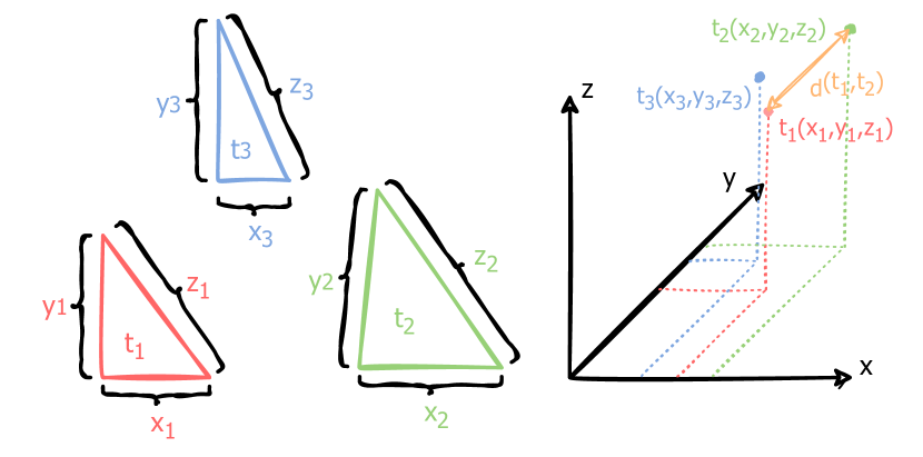
Figure 4: Triangle distance metric based on the sorted lengths of individual edges.

3.3 K-means Clustering

We map the triangles into a 3D space according to the lengths of their edges (see Figure 4). Each triangle $t_{i}$ is placed at point $p(x_{i},y_{i},z_{i})$ such that $x_{i},y_{i}$, and $z_{i}$ represent the length of shortest, middle, and longest edge of the triangle $t_{i}$ respectively. In this way, the position of each triangle in the 3D space shows the parameter of the triangle. Similarly, the Euclidean distance $d_{(i,j)}$ between any two triangles $t_{i}$ and $t_{j}$ represents their degree of similarity. The smaller the distance more similar the triangles are, and vice versa. The two similar triangles will lie on the same point, yielding zero distance. Mathematically, the algorithm attempts to minimize the following energy function:

$$\centering F_{d}(M_{f})=\sum_{i=1}^{k}\sum\limits_{\begin{subarray}{c}j=1\\ t_{j}\in c_{i}\end{subarray}}^{n}d(t_{j},t_{i}^{*}),\@add@centering$$ (1)

where $F_{d}(M_{f})$ is the energy function (accumulative distance), $k$ is number of clusters, $n$ is the total number of triangles/patches, $c_{i}$ is the $i^{th}$ cluster, $t_{j}$ is triangle in $c_{i}$, and $t_{i}^{*}$ is the centroid (mean) of cluster $c_{i}$, calculated as:

$$\centering t_{i}^{*}=\frac{1}{|c_{i}|}\sum_{t_{j}\in c_{i}}t_{j}.\@add@centering$$ (2)

Similarly, $d(t_{j},t_{i}^{*})$ is the value indicating the degree of dissimilarity between $t_{j}$ and $t_{i}^{*}$, which is calculated as square Euclidean distance between their positions ($p(x_{j},y_{j},z_{j})$ and $p^{*}(x_{i}^{*},y_{i}^{*},z_{i}^{*})$, respectively) in our 3D space. Mathematically,

$$\centering d(t_{j},t_{i}^{*})={|x_{j}-x_{i}^{*}|}^{2}+{|y_{j}-y_{i}^{*}|}^{2}+{|z_{j}-z_{i}^{*}|}^{2}.\@add@centering$$ (3)

In other words, $|x_{j}-x_{i}^{*}|$, $|y_{j}-y_{i}^{*}|$, and $|z_{j}-z_{i}^{*}|$ are the differences between the shortest, middle, and longest edges of the two triangles, respectively. An abstract view of our clustering scheme is presented in algorithm 2.

Data: $M_{f},k,T$

Result: $Labels,WithinClusterDistances$

1:  $Matrix{[n\times n]}\leftarrow Virtual3Dspace$

2:  for each $cell(i,j)$ of $Matrix{[n\times n]}$ do

3:     $cell(i,j)\leftarrow d(t_{i},t_{j})$  // Dissimilarity between $t_{i}$ and $t_{j}$ (calculated via Equation 3).

4:  end for each

5:  $\left[Labels,WithinClusterDistances\right]\leftarrow\textit{K-means }(Matrix{[n\times n]},k)$

6:  Label each triangle according to its $Cluster$ number.

7:  return $\left[Labels,WithinClusterDistances\right]$

Algorithm 2 Clustering

For clustering, we first create a $n\times n$ matrix where each cell $(i,j)$ contains the value of $d(t_{i},t_{j})$ calculated via Equation 3. Then, we apply K-means clustering to the matrix, which classifies the triangles into $k$ clusters, where the user specifies $k$. Each triangle is labeled with its value of $k$ representing its class. For each cluster, the central triangle is calculated via Equation 2. Then remeshing operators are applied to minimize the distance, defined with Equation 3, of any triangle of the cluster to its cluster’s central triangle.

Convergence point and clustering error:

The convergence point of algorithm 1 is reached when the maximum value of the within-cluster distances (Equation 4) reaches a given threshold. This maximum value indicates the highest difference among the triangles in the same cluster. We define our clustering error of any triangle as the Euclidean distance from its cluster’s central triangle. The maximum error $(Error_{max})$ and mean error $(\overline{Error})$ can be calculated from Equation 3 as follows.

$$\centering Error_{max}=max(d(t_{j},t_{i}^{*})),\forall 1\leq i\leq k,t_{j}\in c_{i},\@add@centering$$ (4)

and,

$$\centering\overline{Error}=mean(d(t_{j},t_{i}^{*})),\forall 1\leq i\leq k,t_{j}\in c_{i}.\@add@centering$$ (5)

3.4 Remeshing Pipeline

Local operators (edge flip, edge collapse, and vertex translation) are used for surface remeshing (see algorithm 3). The objective of remeshing is to minimize the distances between the triangles in each cluster (i.e., to make them similar). The objective is achieved by minimizing the energy function defined with Equation 1. The algorithm works as follows: starting with a cvt-initialized mesh, the algorithm first improves the regularity of vertices by making its valency (number of adjacent edges) optimal. Edge flip operators make the valencies of the vertices equal to or near 6 (a regular vertex). Regular vertices converge quickly during surface remeshing (Khan et al., 2022; Vidal et al., 2015).

As stated in subsection 3.3, the shape of each triangle is mapped into a single point in a virtual 3D space. The central triangle of each class of triangles (from surface mesh), which is calculated using Equation 2, is presented by a central point of the cluster (in the virtual 3D space). The distance from each triangle to the corresponding centroid is calculated using the degree of similarity between the two triangles (Equation 3). Making triangles similar in the surface mesh brings the corresponding points in 3D space closer to the central point. To minimize this distance, the algorithm applies direct remeshing operators, including edge flip, edge collapse, and vertex translation.

Edge flip and collapse:

Remeshing algorithm (algorithm 3) is called from the main algorithm (algorithm 1). For the first iteration of the main algorithm, the edge flip and edge collapse operators are applied in algorithm 3 if this improves the similarity values. Next is the vertex translation, which is applied in each iteration.

Data: $M_{s},k,T,Itr$

Result: $M_{f}$ with k classes of identical triangles

1:  if Itr=1 then

2:     $M_{f}\leftarrow ValenceOptimization(M_{s})$

3:     if CollapseImprovesClusteringDistance then

4:        $\mathrm{Collapse}()$

5:     end if

6:     for each edge $e_{i}\in M_{f}$ do

7:        if EdgeFlipImprovesClusteringDistance then

8:           $\mathrm{EdgeFlip}()$

9:        end if

10:     end for each

11:  end if

12:  for each edge $e_{i}\in M_{f}$ do

13:     Calculate required new length of $e_{i}$  // i.e., difference from cluster’s center via Equation 3

14:     Calculate its pressure on both side vertices

15:  end for each

16:  for each vertex $v_{c}\in M_{f}$ do

17:     Calculate pressure from each adjacent edge

18:     Calculate new position $p^{*}$  // i.e., mean of the pressures from adjacent edges (see Equation 6)

19:     if ShapeIsPreserved then

20:        Translate $v_{c}$ to new position $p^{*}$

21:     end if

22:  end for each

23:  return $M_{f}$

Algorithm 3 Remeshing

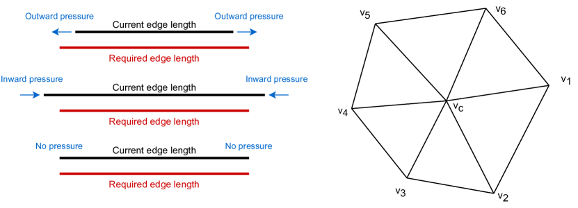
Figure 5: Pressure calculation for vertex translation. Left: three cases of pressure direction. The current edge length is increased/decreased/kept unchanged depending on the required edge length. Right: 1-ring neighborhood of a vertex $v_{c}$ and calculation of accumulative pressure.

Vertex translation:

Vertices are translated using algorithm 3. The algorithm requires information on whether to increase or decrease the edge length (see Figure 5 (left)). Equation 3 puts pressure on each edge, indicating the magnitude of change in edge length to make it similar to the corresponding edge of the cluster’s central triangle. The pressure is divided on both side vertices of each edge. Since each vertex is connected to multiple edges, it is affected by pressure from different side edges (see Figure 5 (right)). Figure 5 (right) shows 1-ring neighborhood of vertex $v_{c}$. Each vertex $v_{i}$ from the neighborhood of $v_{c}$ puts pressure on $v_{c}$, attempting to bring it to a new position $p_{i}$. For a vertex with $n$ adjacent vertices, Equation 6 calculates the average of $n$ new positions to find the final position $(p^{*})$ for $v_{c}$. The above steps are applied iteratively until the algorithm converges.

$$\centering p^{*}=\frac{1}{n}\sum_{i=1}^{n}p_{i}.\@add@centering$$ (6)

To ensure geometric preservation and avoid possible deformation, we put restrictions on vertex translation. The vertex translation is only allowed if new position $(p^{*})$ is inside the predefined limit. In case it lies outside, the value of $p^{*}$ is recalculated as a middle point between $p^{*}$ and the current position of the vertex. This limit is defined on each side of the surface. Typically, this limit is kept as $0.25^{th}$ of the mean edge length. However, for a quicker convergence, this value can be increased.

3.5 Puzzle and Assembling

we aim to generate reconfigurable puzzle segments from the input surface. To ensure that segments are reconfigurable, we thicken the surface by adding a new surface layer and connecting it with the existing one resulting in a triangle patch with user-defined thickness as shown in Figure 6. The thickened triangle patches are processed for female connections (holes), allowing interconnection with other segments via a hinge joint connector.

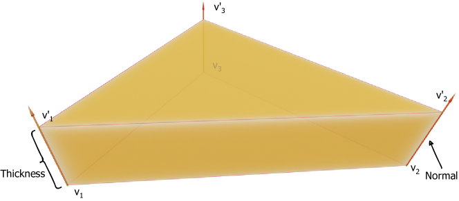
Figure 6: The individual triangular patch is thickened along the vertex normals.

Thickening:

For creating an external surface layer, we calculate the vertex normals (irrespective of its clustering). The vertex normal is calculated as the mean of the normals of the adjacent triangles. Next, we insert a new vertex ($v^{\prime}_{1}$, $v^{\prime}_{2}$, $v^{\prime}_{3}$) on the normal of each vertex at a distance of user-given thickness. We connect the corresponding vertices, which make quad patches at three sides of the thickened triangle (see Figure 6). This thickened triangle patch is a closed mesh having two triangles i.e., a bottom triangle ($v_{1}$, $v_{2}$, $v_{3}$) laying on the inner layer and an upper triangle ($v^{\prime}_{1}$, $v^{\prime}_{2}$, $v^{\prime}_{3}$) laying on the outer layer and three quads. Finally, for a unique thickened triangle for each cluster, we calculate the mean of possible variations in the vertices’ normals.

The new vertices ($v^{\prime}_{1}$, $v^{\prime}_{2}$, $v^{\prime}_{3}$) added for the thickness also define the curvature. If we use the vertex normal, the outer layer ($v^{\prime}_{1}$, $v^{\prime}_{2}$, $v^{\prime}_{3}$) of each part (thickened triangle) will be bigger, equal, or smaller than inner one ($v_{1}$, $v_{2}$, $v_{3}$) depending upon its position on the surface, which can be concave, planar or convex. Face normal, on the other hand, yields similar sizes for both layers without regard to curvature.

Figure 7 shows the thickened triangle patches using different approaches (see 7(a) and 7(b)) on a full surface. In the case of face normals (perpendicular extrusion), for each triangle patch, the inner and outer layers are the same; therefore, there is some free space between them in the composed model. We use the vertex normal instead, which enables us to fill those spaces. Since the outer layer is dependent on curvature, the thickened triangles from the same class might have different sizes of the outer layer. To handle this issue, we find mean curvature for all parts in each class to finalize the positions of the new vertices ($v^{\prime}_{1}$, $v^{\prime}_{2}$, $v^{\prime}_{3}$). The three quads on the sides of the triangle are further processed for holes.

Subdivision smoothing gives even better results (see 7(c)). The inner and outer triangle surface patches are linked with quad strips linking the corresponding vertices. The number of vertices along each edge is defined by the level of the applied subdivision smoothing. These thickened triangle patches are further processed for connection holes before it is ready to be printed.

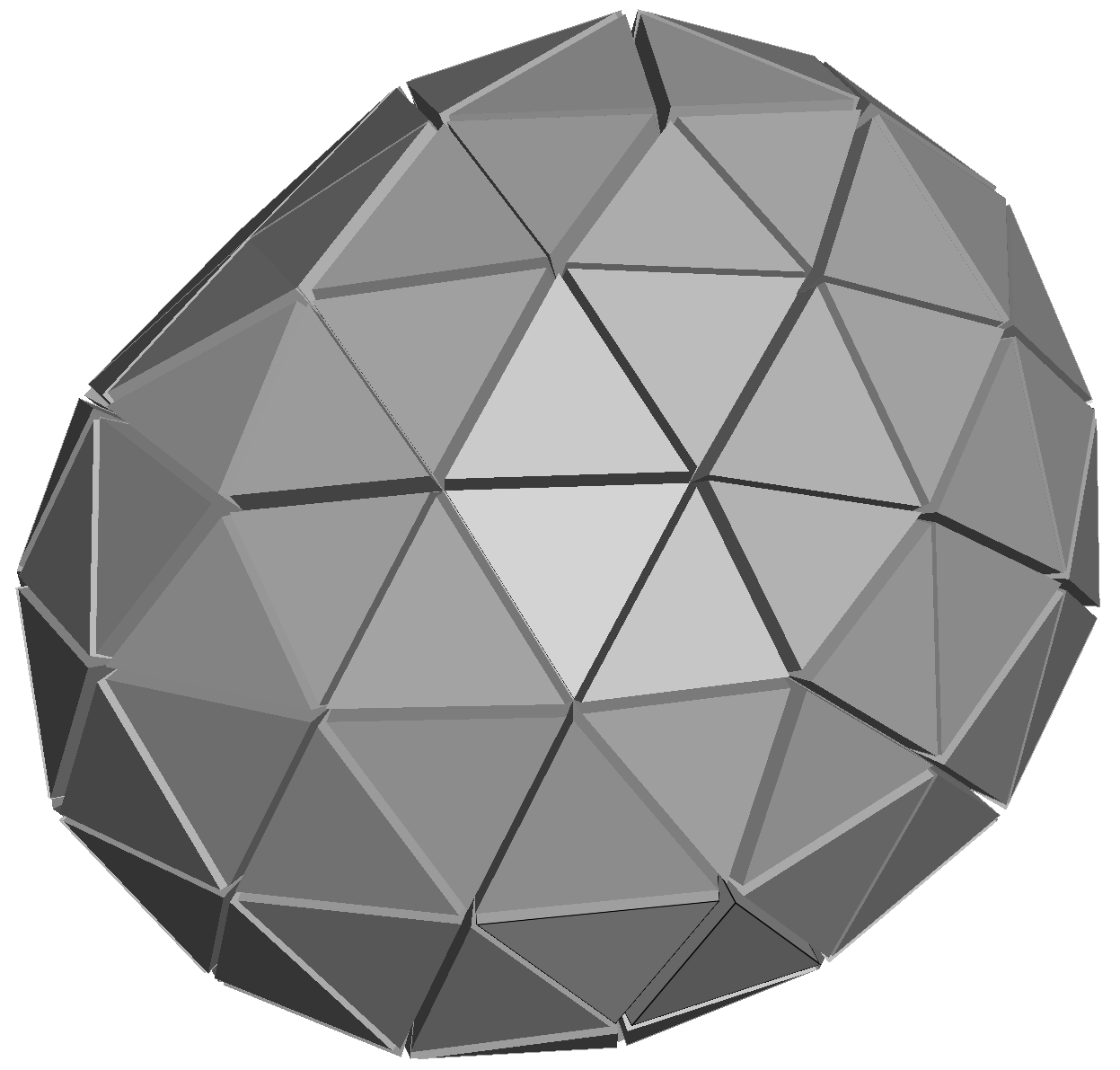
(a) Perpendicular extrusion.

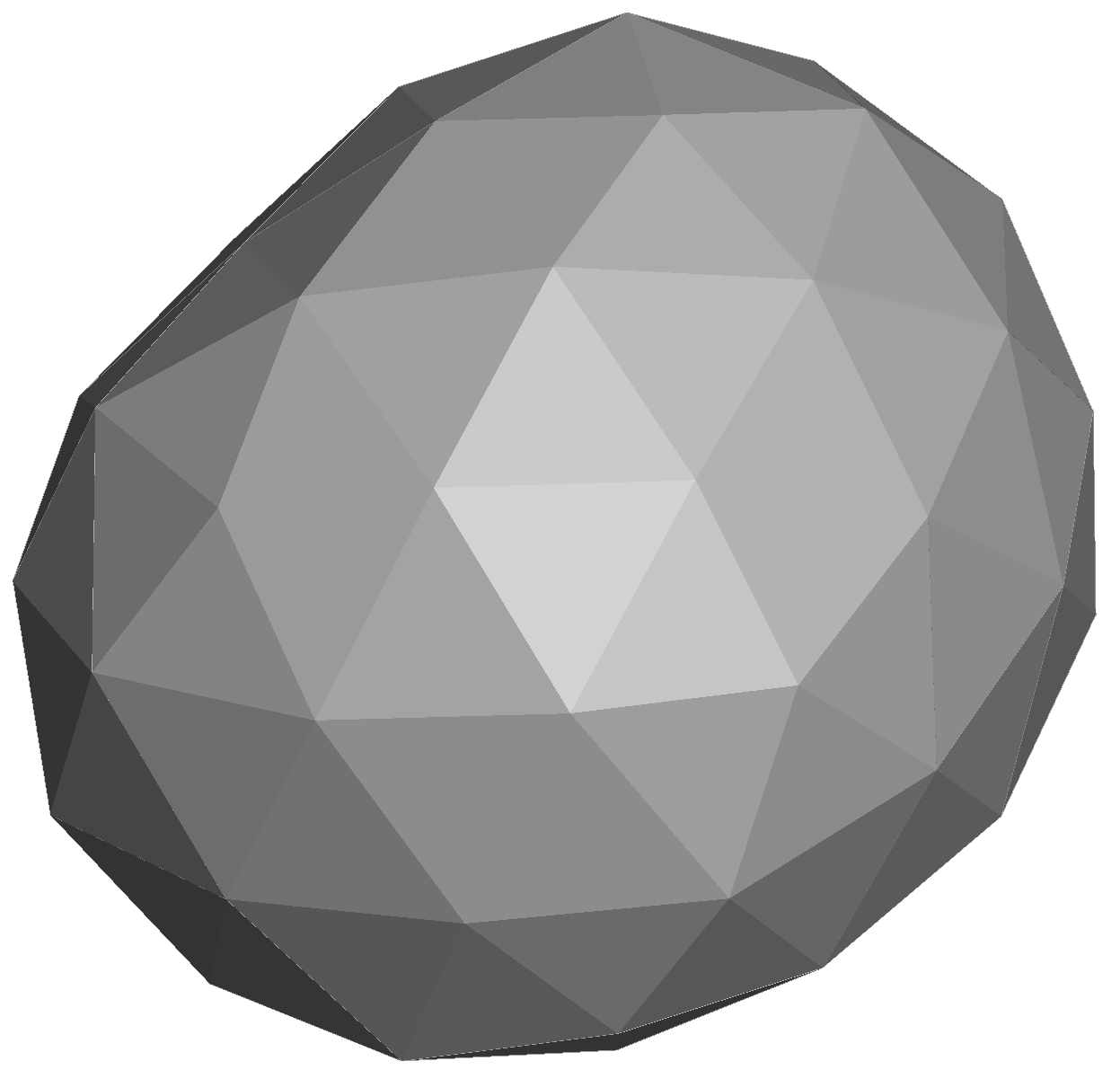
(b) Curvature-aware

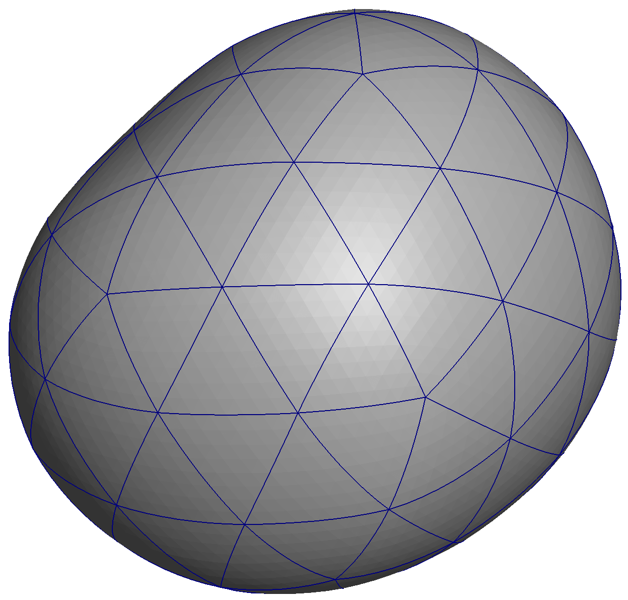
(c) After smoothing.

Figure 7: Thickness layer: 7(a): The outer layer is created via face normal. 7(b): The outer layer is created via the vertex normal (Curvature-aware extrusion). 7(c) Smoother with subdivision.

Connecting structures:

Since the thickened triangle patches’ sides differ significantly between the planar and curved triangle patches, we designed separate procedures for generating connecting parts for them. The connecting structures consist of holes in the thickened triangular patches and hinge joint connectors (see Figure 8).

Planar triangular patch: To preserve the structural strength of individual pieces and provide some clearance tolerance for the connecting structures, we create holes parallel to the inner and outer surfaces. To achieve this, we calculate the center point ($c$) of the quad extruded from vertices (e.g., $v_{1}$ and $v_{2}$) perpendicularly to the inner surface touching the outer surface (see top image in Figure 9). We define the position of vertices $q_{1},\ldots,q_{4})$, which determine the hole boundary, according to the size of the hinge joint connector defined by the user. Next, we extrude the quad defined with vertices $q_{1},\ldots,q_{4}$ inwards according to the size of the hinge joint connector. We remesh the outer side surface by connecting original vertices $v_{1},v_{2},v_{3},v^{\prime}_{1}v^{\prime}_{2},v^{\prime}_{3}$ with newly created vertices $q_{1},\ldots,q_{4}$. The top image in Figure 9 outlines the process. The same process is repeated for all three sides of the triangular patch.

Curved triangular patch: Creating holes in the curved triangular patches is a bit more challenging. We first align the triangular patch so that the vertices $v_{1},v_{2},v_{3}$ lie on the XY-plane. Next, we calculate a projection point $d$ of the midpoint between vertices (e.g., $v_{1}$ and $v_{2}$) $c$ to the outer edge of the same side (see the bottom image in Figure 9). We define the hole center point $e$ at the half-thickness distance $w_{h}$ from point $d$ to $c$. We define the positions of vertices $q_{1},\ldots,q_{4}$, which determine the hole boundary, with respect to the center point $e$ and the size of the hinge joint connector, defined by the user, on a plane defined with vertices $v_{1},v_{2},d$. The quad defined with vertices $q_{1},\ldots,q_{4}$ is then extruded inwards according to the size of the hinge joint connector. The side surface of the thickened curved triangular patch is remeshed by incorporating the vertices $q_{1},\ldots,q_{4}$. The same process is repeated for all three sides of the triangular patch.

Hinge joint connectors: The holes are identical for all triangles. Similarly, considering the box-like shape of the created holes defined by eight vertices, we generate appropriate hinge joint connectors for all edges to connect triangles with each other. The assembled hinge joint connector fits inside two holes (with some spacing to compensate for the printer inaccuracies). Its size is determined by the user, who must also consider the possible overlaps of the holes within the individual triangular patch if they are too big. The two parts of the hinge joint connector are printed with a resin material (similar to triangles). However, inside the connector is a metal rod (see Figure 8).

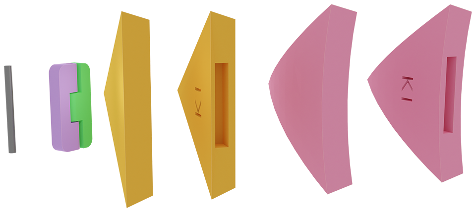
Figure 8: Puzzle parts: A thickened triangle with and without holes and a hinge joint connector.

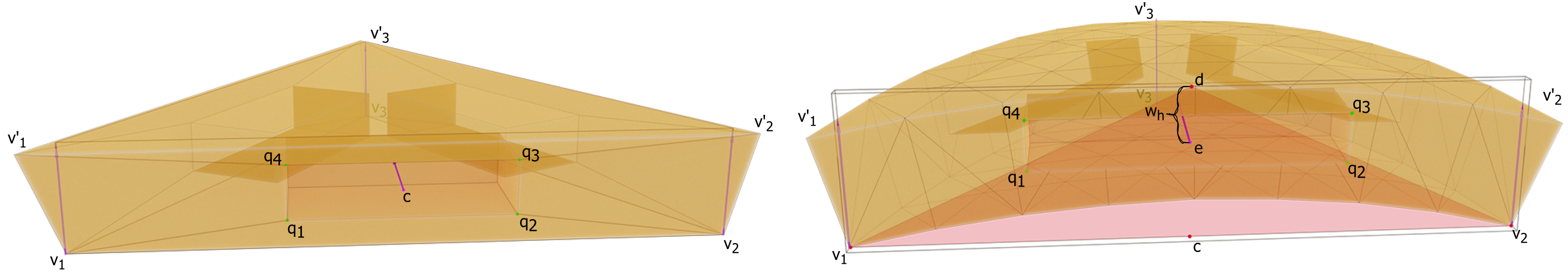
Figure 9: Outline of hole generation process for connecting neighboring planar (left) and curved (right) triangle patches.

3.6 Flexibility and extendability

We mainly generate puzzle parts from planar triangular patches. However, we also implemented the support for curved triangles. Similarly, our technique also provides the option of merging triangles into other polygonal structures, which reduces the puzzle’s complexity if intended by the puzzle designer.

Sub-division and Smoothing

The mesh complexity has been reduced during the initialization step of our algorithm. However, the simplified mesh has a rigid surface with discrete planar triangles. To improve surface smoothing, we follow the approach by Loop (1987) to smooth the mesh by subdivision of triangles. The curved triangles are easy to assemble and provide a smoother surface. However, it is very hard to improve their isometric decomposition. Therefore, we only create curved triangles and apply classification with a higher number of $k$.

Curvature-aware patch classification:

With subdivision, each planar triangle patch is divided into 64 triangles (in 3 iterations $4^{3}$), making a curved patch. We store the boundaries of each patch and calculate its curvature. Next, we apply patch-wise classification, which applies not only the parameter but also the curvature. For curvature-aware patch classification, we add a $4^{th}$ dimension $w$ to Equation 3 as follows:

$$\centering d^{\prime}(t^{\prime}_{j},t_{i}^{\prime*})={|w_{j}-w_{i}^{*}|}^{2}+{|x_{j}-x_{i}^{*}|}^{2}+{|y_{j}-y_{i}^{*}|}^{2}+{|z_{j}-z_{i}^{*}|}^{2},\@add@centering$$ (7)

where $t^{\prime}_{j}$ and $t_{i}^{\prime*}$ are the $j^{th}$ curved triangle in $i^{th}$ class, and center of the cluster, respectively. To calculate $w$, we find the center of the planar triangle (formed by three corner vertices of the curved triangle) and the center of the central sub-triangle of the subdivided curved triangular patch and calculate the square Euclidean distance between them. The curvature-aware patch classification gives smoother results. However, if two patches have an abrupt change from concave to convex (or vice versa), the uniform width calculation for patch thickness becomes challenging.

Merge Triangles

For further flexibility, the user can also choose to merge triangular patches into convex polygonal patches (full or parts of the pentagons and Hexagons). Depending upon user choice, we provide different merging options, including two, five, six, or seven triangles. The merging strategy can minimize the puzzle’s complexity.

4 Experimental Results

This section evaluates Dr. KID on different organic shapes such as SARS-CoV-2 virions from the Electron Microscopy Data Bank under id EMD-33297 (Nguyen et al., 2022), mitochondria from the UroCell Dataset (Žerovnik Mekuč et al., 2020, 2022), and cell nuclei from the WTC-11 hiPSC Single-Cell Image Dataset v1 (Viana et al., 2023). We show some assembled models of these shapes and compare them with their 3D models in Figure 13. The proposed algorithm is implemented in C++ and tested on Intel(R) Xeon(R) Gold 6230R CPU $2\times 2.10$ GHz with 156 GB RAM and $64$ bit Windows 10 operating system.

4.1 Validation

In this section, we present empirical results to validate the applicability and effectiveness of our algorithm. We calculated the actual cluster error and a relative error, i.e., percentage of the mean edge denoted as $\%(e)$. The relative error gives an easy judgment of the accuracy as it considers the actual length. Typically, the remeshing algorithms and isometric decomposition need only negligible (acceptable) geometric loss. We calculate the geometric loss in the percentage of bounding box value of the Hausdorff distance (Bartoň et al., 2010). As stated in subsection 3.1, our algorithm generates a raw mesh ($M_{i}$), which is preprocessed and simplified to $M_{s}$. The simple mesh $M_{s}$ is then iteratively remeshed consecutive with K-means clustering to reach a given threshold. Additionally, there may be some geometric loss during mesh simplification $d_{H}(M_{i},M_{s})$ and in clustering/remeshing $d_{H}(M_{s},M_{f})$. Figure 10 shows the clustering results for different models. Table 1 shows quantitative results, including the geometric loss, efficiency, classification error, and the number of iterations. Observing the numerical results, we can conclude that the geometric loss during the clustering is smaller than the geometric loss in simplification. However, there is a trade-off between the clustering threshold $T$ and geometric loss ($d_{H}$). The threshold $T$ given to the algorithm shows the limit of acceptable clustering error. Since we are dealing with variable-sized models, the $T$ shown in the paper is the percentage of the mean edge length. The algorithm iterates until the errors are under the threshold limit. Therefore, the average clustering error is smaller than $T$ (see Figure 11, and Figure 12).

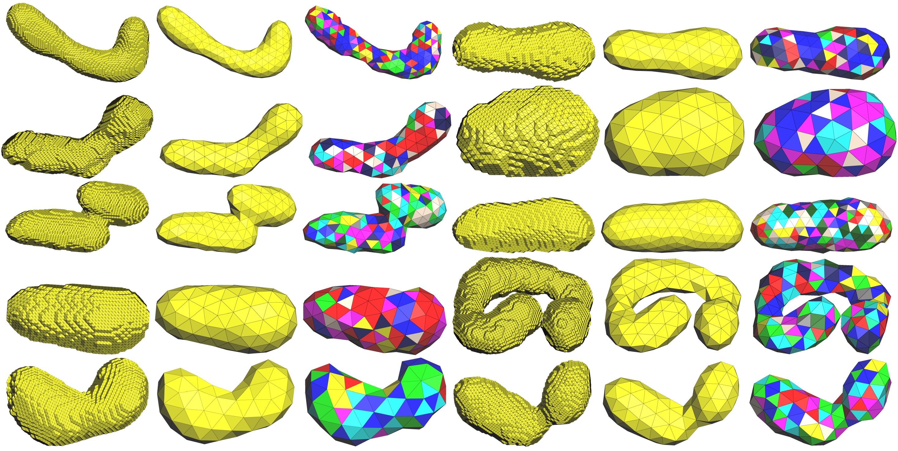
Figure 10: Clustering results of 10 different models. From top left to bottom right, we name the models $M1$ to $M10$. For each model, the three sub-figures (from left to right) are mesh generated from the 3D shape ($M_{i}$), the simplified mesh ($M_{s}$), and our results ($M_{f}$). The corresponding numerical results are given in Table 1.

The algorithm is iterative and proceeds toward its convergence by minimizing the clustering error and the value of the accumulative energy function. Figure 11 plots the energy minimization (Equation 1) and shows the convergence of the algorithm with the number of iterations. The clustering errors also decrease as the algorithm iterates.

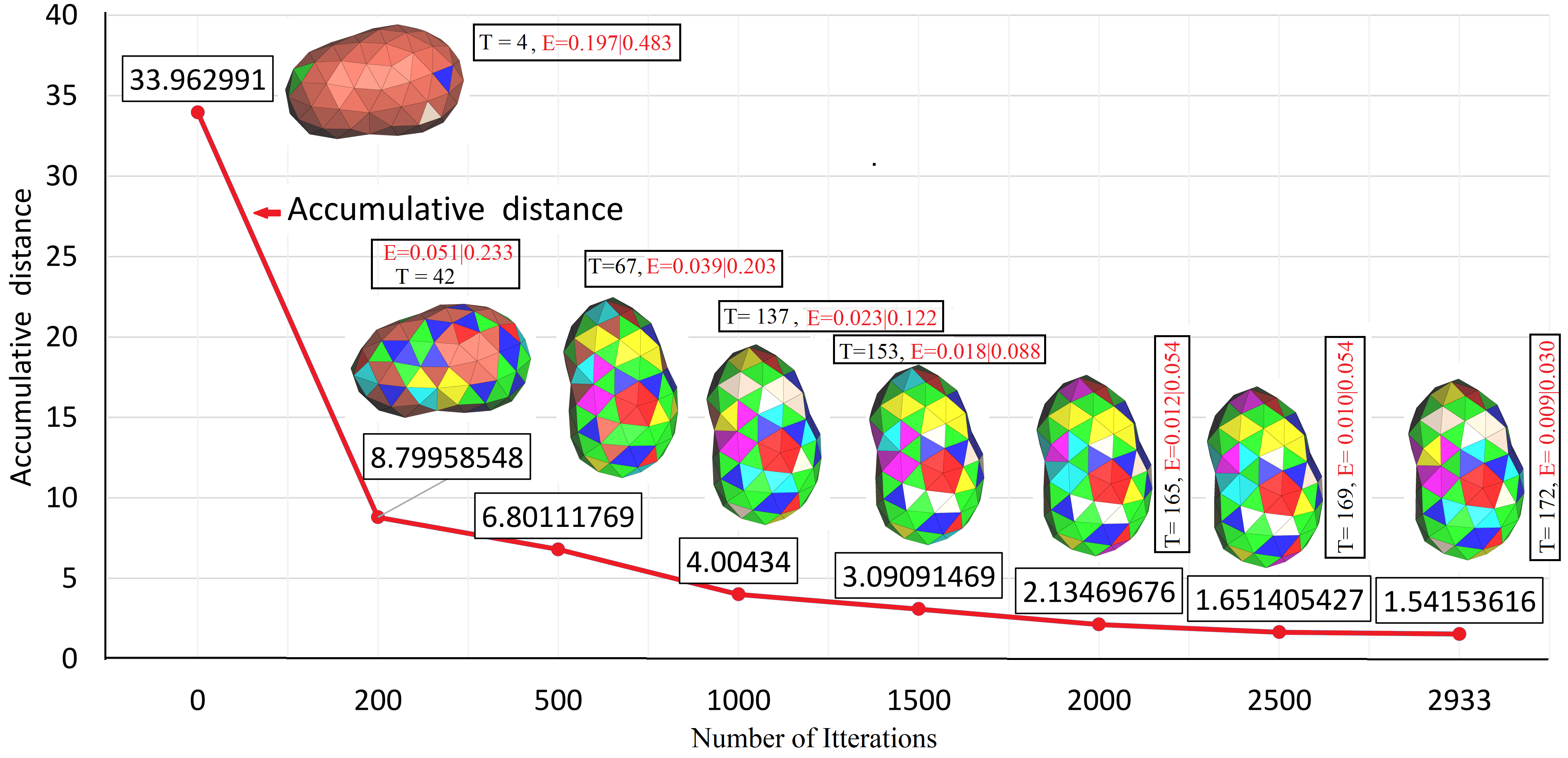
Figure 11: Minimization of the accumulative distance (i.e., energy function Equation 1) with number of iterations. Here $T$ presents the number of triangles with error smaller than the threshold (0.03). $E$ represents the clustering error (mean|max). The brown-colored triangles have errors above the threshold.

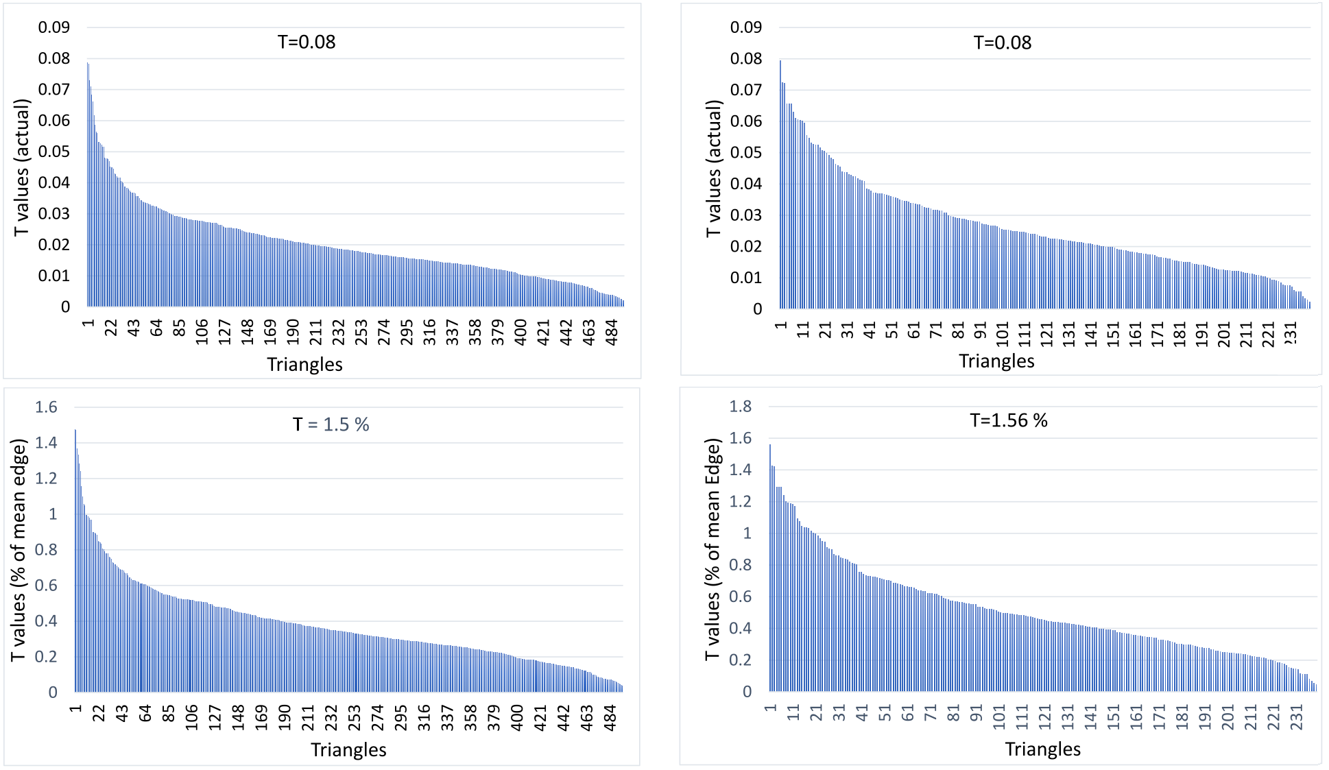
Figure 12: Histogram of clustering error for two models. Top actual values and bottom percent values. Left: M1 with an average error of $0.38\%$ for 496 triangles. Right: M2 with an average error of $0.53\%$ for 240 triangles. The values are calculated as a percentage of the mean edge length. Here x-axis represents the triangle number, whereas the y-axis shows the clustering error (distance from the cluster center in $\%$ of mean edge length).

4.2 Printing Results

The prototypes were printed using two 3D printers: Stratasys J750, a high-resolution full-color 3D printer and FormLabs Form3 SLA 3D printer. All the hinge joint connectors and most of the models were printed using Stratasys 3D printer. Only triangles of the big SARS-CoV-2 virion membrane model were printed using the FormLabs printer. The printing resolution and precision of the FormLabs printer are not good enough for the final model to be assemblable. These 3D fabrication results are prototypes validating the plausibility of our method. The envisioned production will use the molding process, where our low demand on the number of required molds will secure the production scalability.

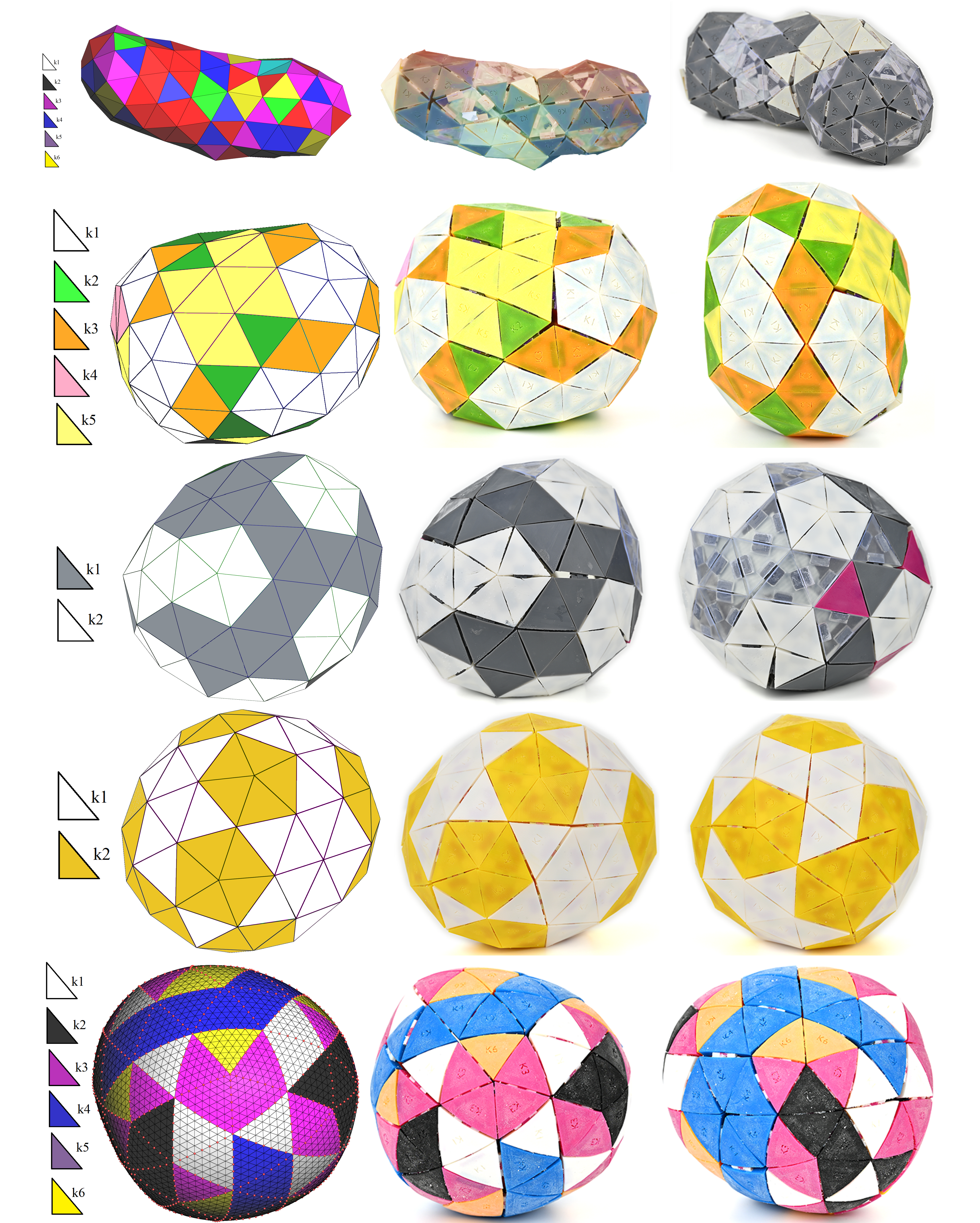
Figure 13: Printed results. Top to bottom: Mitochondria outer membrane, cell nuclei membrane, and three models of SARS-CoV-2 virion membranes. The bottom row shows a model with curved triangle patches. The labels on the left column indicate the values of $k$ and segment colors. The number of colors of the printed models in the first and third row is smaller than the number of classes due to the limited colors available for 3D printing.

The 3D-printed results of several models are displayed in Figure 1 and 13. Figure 13 also shows how the 3D models relate to their 3D-printed versions. We show that the printed results are similar to the original models. However, the tight connectors (hinge joints) are difficult to use for creating reconfigurable joints during the assembly phase. Therefore, we used loose hinge joints, which create gaps near the vertices with valence $\geq 7$. The size of the gaps also depends on the printer’s accuracy.

Classification of the curved patches:

In addition to planar triangles, Dr. KID can be used for curved triangular patches. Figure 14 shows the results of a model composed of curved triangular patches. For curved triangular patches, we only provide the classification of the patches without any further remeshing. To reach a suitable classification, users must find an optimal combination between $T$ and $k$. For example, the model in Figure 14 can classify all the patches (116) with $T=7.5\%$ if $k=6$. However, this patch-wise classification can be achieved with a lower threshold $T=3.75\%$ if we set $k=10$. The last row in Figure 13 shows a 3D-printed model with curved triangular patches.

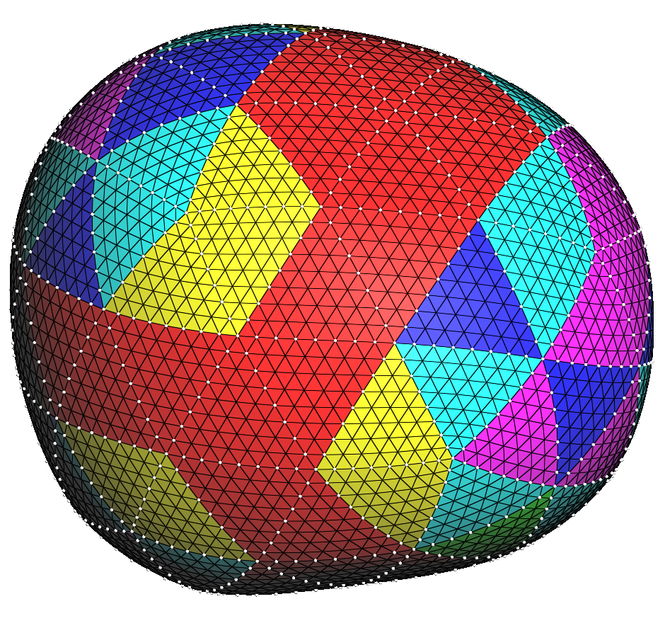
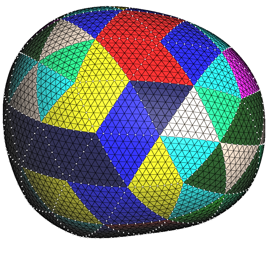
Figure 14: Patch-wise classification: Left: Clustering of planar triangles with $k=2$, $T=0.01\%$, Middle: Patch-wise classification with $k=6$, $T=7.50\%$, Right: $k=10$, $T=3.75\%$

4.3 Comparison with related methods

In the domain of biological structures, there is no standard algorithm that can be used for comparison with our approach. However, there are few articles in other domains. We choose a most recent article (Liu et al., 2021) for a short comparison using two models. Figure 15 shows the comparative results. The results show that our method gives smoother results with a lower $d_{H}$. Moreover, our method is faster.

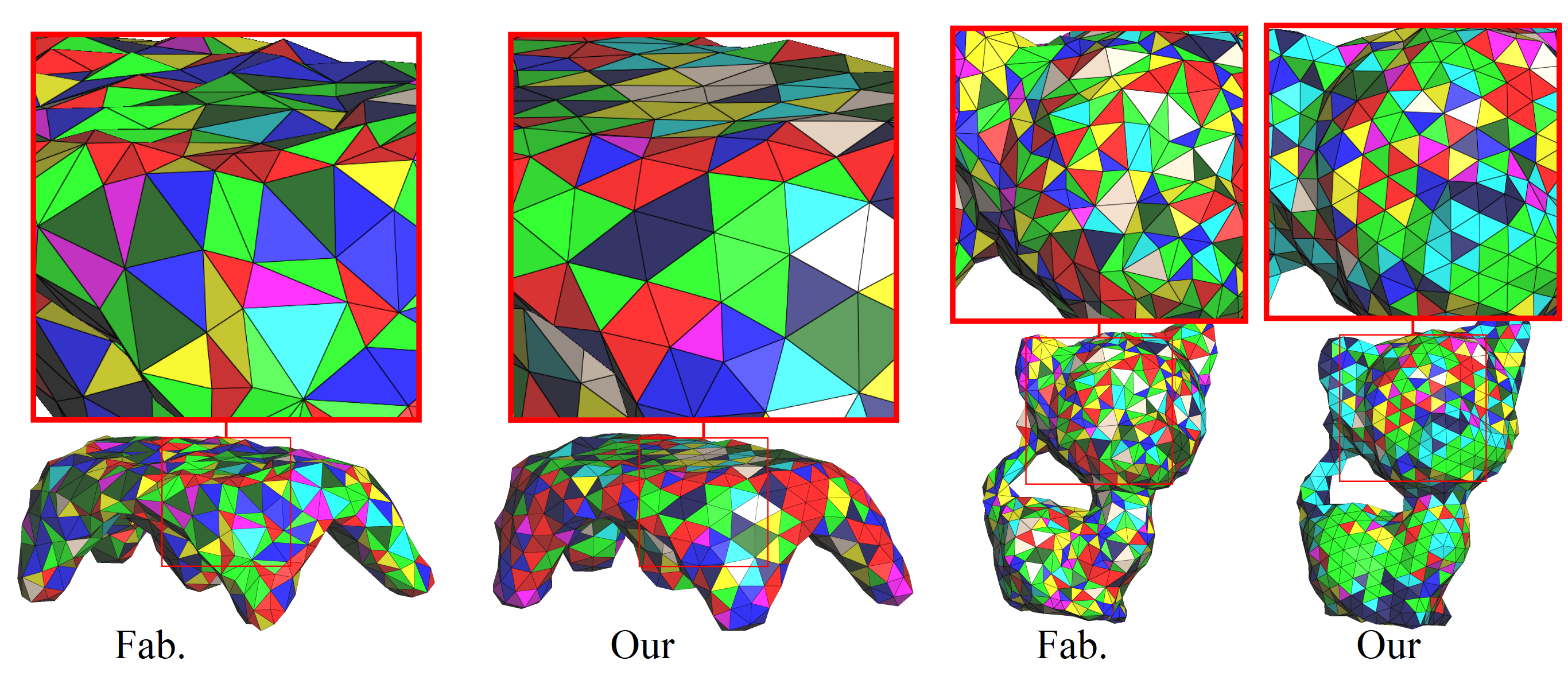
Figure 15: Comparison with a previous method (Liu et al., 2021) for k=9. Left (in each pair): Fabrication method (Liu et al., 2021) with $d_{H}(\%bb)=1.62$ and $1.33$, and with time taken 85.6 minutes, and 91.2 minutes. Right (in each pair): Our with $d_{H}(\%bb)=1.53$ and $1.31$, and with time taken 38 seconds and 27 seconds.

Table 1: Quantitative results. Here $M_{i}$ is the input mesh, $M_{s}$ is the simplified mesh, and $M_{f}$ is the resulting mesh of our method. $T$ is user given threshold, and $d(t,t^{*})$ is the average Euclidean distance from the cluster centers. Here, $\overline{Length(e)}$ is the mean length of edges, $\%(e)$ is the percent value of the mean of $\overline{Length(e)}$, $d_{H}$ is calculated in $\%$ bounding box. $\overline{Error}$ is the mean clustering error calculated via Equation 5.

Figure #/Model	# Faces	# Vertices	k	T	$\overline{Length(e)}$	$\overline{Error}$	$d_{H}(M_{i},M_{s})$	$d_{H}(M_{s},M_{f})$	$d_{H}(M_{i},M_{f})$	Time	Iterations
	$M_{i}/M_{s}/M_{f}$	$M_{i}/M_{s}/M_{f}$		actual/$\%(e)$		actual/%(e)	mean/max	mean/max	mean/max	Sec.	#
Figure 10/ M1	21280/500/496	10642/252/250	7	0.08/1.50	5.33	0.020/0.382	1.33/2.55	0.62/1.77	3.38/1.25	248	7893
Figure 10/ M2	10460/242/240	5232/123/122	9	0.08/1.57	5.08	0.026/0.519	2.60/4.33	0.49/1.87	2.46/4.44	15	993
Figure 10/ M3	14048/264/262	7026/134/133	8	0.06/1.03	5.79	0.018/0.317	1.61/3.62	0.65/2.16	1.50/3.72	41	2385
Figure 10/ M4	5968/172/172	2986/88/88	7	0.08/1.53	5.20	0.025/0.475	0.50/1.47	0.72/3.27	0.83/2.71	15	1546
Figure 11/ M4b	5968/172/172	2986/88/88	7	0.03/0.57	5.21	0.009/0.172	0.50/1.47	0.83/3.65	0.91/3.06	42	2933
Figure 10/ M5	16072/374/372	8038/189/188	11	0.09/1.56	5.74	0.028/0.490	0.22/0.95	0.50/2.50	0.51/2.05	59	2349
Figure 10/ M6	9612/416/416	4808/210/210	11	0.09/2.17	4.14	0.032/0.775	0.23/0.71	0.83/3.15	0.98/3.45	48	1962
Figure 10/ M7	7280/196/196	3642/100/100	8	0.08/1.44	5.57	0.023/0.416	0.39/1.00	0.90/3.37	0.88/3.48	33	2894
Figure 10/ M8	21288/400/396	10646/202/200	11	0.09/1.39	6.49	0.023/0.355	0.29/0.90	0.67/2.83	0.65/2.71	101	5134
Figure 10/ M9	10380/156/156	5192/80/80	6	0.07/0.98	7.12	0.023/0.320	0.39/1.07	0.90/3.20	0.84/3.58	33	3170
Figure 10/ M10	11496/196/196	5750/100/100	8	0.08/1.20	6.68	0.035/0.520	0.36/1.72	0.67/2.38	0.72/2.57	17	1933
Figure 13/top	4807/172/170	2406/88/87	6	17.3/1.89	914	6.968/0.762	0.34/1.23	0.967/3.20	0.85/2.34	22	987
Figure 13/N-cell	83040/136/136	41522/70/70	6	0.50/1.70	29.32	0.180/0.613	1.33/0.49	1.24/2.94	2.11/4.17	51	4732
Figure 14/left	320/116/116	162/60/60	2	0.02/0.01	160	0.007/0.004	0.50/1.04	1.10/3.32	1.93/4.70	144	8349

5 Discussion

Dr. KID is the novel system for the physicalization of organic shapes. It can be an effective tool for learning objects’ physical properties and structure by providing a physical shape. The physicalization starts from a 3D shape and ends with a physical model assembled from reconfigurable parts. We provide a simple physical structure of small biological structures so users can assemble and see the basic structure. An abstract view of the structure is provided to the audience as a physical model, whereas the detailed functionalities of these models are not explored. We aim to attract the audience by providing a simple reconfigurable model. The models can also play a vital role in scientific museums or awareness conferences for public outreach.

The key goals of Dr. KID are: (1) to reduce cost by creating isometric segments, (2) to provide a puzzle-like reconfigurable physical model, and (3) to preserve the shape and curvature of the input shape.

For the isometric decomposition, we triangulate the surface mesh and design an energy function to increase the degree of similarity of triangles belonging to the same class. We proposed a simple yet novel method of computing similarities between triangles. Previous methods (Liu et al., 2021; Singh and Schaefer, 2010; Fu et al., 2010) used the vertex distances of two aligned triangles, so they need optimization to find the best alignment transformation. On the other hand, our method does not require this optimization of finding the best alignment transformation and is, therefore, computationally efficient.

Figure 11 shows the minimization of this energy by increasing the similarities among the triangles. For this energy minimization, we used surface remeshing, which can preserve the input shape. Figure 15 shows that our method provides smoother and more accurate results than the existing method. For puzzle-like assembly, we provide an automatic thickness and hole creation strategy. The thickness is created in the direction of vertices’ normals and thereby preserves the curvature during assembly. If there is a small error in the curvature estimation, it can be compensated for by the freedom of hinge joint rotation.

The isometric decomposition provides a cost-effective solution for physicalization using injection molds or 3D printing, the former especially if a large quantity is demanded. Similarly, for a small number of prints, since we need to process each patch for holes and hinges, the isometric patches are easy to handle, where we process only one patch from each class of isometric patches.

The holes and hinge joints provide a connection between the triangles. The hinge joints can provide a certain degree of freedom to recover the possible geometric loss/error in curvature during the puzzle parts generation. In other words, the angle between the two faces (triangles) can be increased/decreased due to the use of hinge joints. Figure 13 shows our printed results which show a similar visual result to the input model.

The algorithm converges when the degree of similarities among the triangles reaches its threshold. In other words, if the clustering error goes below an error threshold. Typically, the parameters, including threshold (T), the k value, and the $d_{H}$ have a trade-off. Selecting a smaller value of $T$ will increase the $d_{H}$ or require a higher value of $k$. If we keep $d_{H}$ adjustable by the algorithm and set higher values of $T$ and $k$, the algorithm can reach convergence with a relatively smaller value of $d_{H}$. However, no mechanism exists to automate the optimal balance among these three parameters. After convergence, the maximum error cannot exceed a given threshold in each class of similar triangles. For example, Figure 12 shows that only a few triangles are close to the threshold.

To support extendability and give smoother results, Dr. KID uses triangle subdivision followed by the classification of the curved triangle patches (Figure 14). For curved patches, we used Equation 7. However, this assumption of curvature estimation may fail in special cases such as complex models.

The scope of our study is limited to a small set of microbes, i.e., tiny models having potato-like curved surfaces (e.g., mitochondria, lysosome, endosomes, cellular nuclei, virus particles, etc. ) without sharp features. Complex structures such as models with sharp edges, models with abrupt changes from concave to convex (for example, brain surface), and generic CAD models are out of the scope of our algorithm. Dr. KID can provide a baseline for several interesting future research directions. For example, modeling realistic biological structures with more detailed information.

6 Conclusion

We have presented Dr. KID , a new physicalization approach for potato-shaped biological structures. Dr. KID generates the surface mesh of the model, which is then decomposed into $k$ types of identical triangle segments. We used a novel mapping function that maps the degree of similarity among the triangles into a virtual 3D space as a distance metric. Next, K-means clustering is applied to classify the triangles into $k$ classes. We used surface remeshing to make all the triangles in the same class similar. The segments are automatically generated as puzzle parts and thickened with hinge joints and female connections to support a reconfigurable assembly. We demonstrate how our approach can be used for 3D printing the prototype models. Dr. KID is considering a cost-reduction approach for the physicalization of small microbes. We hope it to be a practical and useful tool for the community.

Our approach has the following limitations:

• We have evaluated our system empirically with different models, however, we have no theoretical proof of the success in isometric decomposition with an arbitrary model and a given number of $k$, however, the hinge joint connectors compensate for a slight imperfection in the fit.

• Although for our current domain, since the target organic shapes are in several variations, we believe that the geometric loss is acceptable. However, for generic use, the geometric loss should be further considered.

• We only present a short comparison with another fabrication method. However, we did not find any other relevant physicalization algorithms for the biological domain for comparison.

For the future, we are working on designing a specialized mesh generation algorithm to improve accuracy. We also plan to minimize geometric loss during remeshing and extend the algorithm’s scope into other domains. Additionally, we aim to fully automate the process for hinge joint connectors without requiring user-defined dimensions. Furthermore, remeshing the curved patches (Figure 14) to make them isometric is also a future challenge. Finally, we aim to address other parts of the structures apart from membranes.

References

- Bailey et al. [1998] Michael J Bailey, Klaus Schulten, and John E Johnson. The use of solid physical models for the study of macromolecular assembly. Current Opinion in Structural Biology, 8(2):202–208, 1998. ISSN 0959-440X. doi:10.1016/S0959-440X(98)80039-0. URL https://www.sciencedirect.com/science/article/pii/S0959440X98800390.
- Casas and Estop [2015] Lluís Casas and Eugènia Estop. Virtual and printed 3D models for teaching crystal symmetry and point groups. Journal of Chemical Education, 92(8):1338–1343, 2015.
- Bader et al. [2018] Christoph Bader, Dominik Kolb, James C. Weaver, Sunanda Sharma, Ahmed Hosny, João Costa, and Neri Oxman. Making data matter: Voxel printing for the digital fabrication of data across scales and domains. Science Advances, 4(5):eaas8652, 2018. doi:10.1126/sciadv.aas8652. URL https://www.science.org/doi/abs/10.1126/sciadv.aas8652.
- Verdine et al. [2014] Brian N. Verdine, Roberta Michnick Golinkoff, Kathryn Hirsh-Pasek, and Nora S. Newcombe. Finding the missing piece: Blocks, puzzles, and shapes fuel school readiness. Trends in Neuroscience and Education, 3(1):7–13, 2014. ISSN 2211-9493. doi:10.1016/j.tine.2014.02.005. URL https://www.sciencedirect.com/science/article/pii/S221194931400009X. 3rd Latin American Schools on Education and the Cognitive and Neural Sciences.
- Nicolaidou et al. [2021] Iolie Nicolaidou, George Chrysanthou, Marita Georgiou, Christos Savvides, and Stavrini Toulekki. Relationship Between Spatial Reasoning Skills and Digital Puzzle Games. In European Conference on Games Based Learning, pages 553–XIX. Academic Conferences International Limited, 2021.
- Lin et al. [2022] Mei-Ling Lin, Josue David Lopez, Andres Silva, Kinza Ali, Veronica Yvonne Brookshaw, Megan Goldner Martinez, and Dahlia Cavazos Castillo. Cognitive and Socio-Emotional Benefits of Puzzle Working in Older Adults. Activities, Adaptation & Aging, 0(0):1–16, 2022. doi:10.1080/01924788.2022.2120761.
- Moere [2008] Andrew Vande Moere. Beyond the tyranny of the pixel: Exploring the physicality of information visualization. In 2008 12th International Conference Information Visualisation, pages 469–474, 2008.
- Zhao and Moere [2008] Jack Zhao and Andrew Vande Moere. Embodiment in data sculpture: A model of the physical visualization of information. In Proceedings of the 3rd International Conference on Digital Interactive Media in Entertainment and Arts, DIMEA ’08, page 343–350, New York, NY, USA, 2008. Association for Computing Machinery. ISBN 9781605582481. doi:10.1145/1413634.1413696. URL https://doi.org/10.1145/1413634.1413696.
- Jansen et al. [2013] Yvonne Jansen, Pierre Dragicevic, and Jean-Daniel Fekete. Evaluating the efficiency of physical visualizations. In Proceedings of the SIGCHI Conference on Human Factors in Computing Systems, CHI ’13, page 2593–2602, New York, NY, USA, 2013. Association for Computing Machinery. ISBN 9781450318990. doi:10.1145/2470654.2481359. URL https://doi.org/10.1145/2470654.2481359.
- Jansen et al. [2015] Yvonne Jansen, Pierre Dragicevic, Petra Isenberg, Jason Alexander, Abhijit Karnik, Johan Kildal, Sriram Subramanian, and Kasper Hornbæk. Opportunities and challenges for data physicalization. In Proceedings of the 33rd Annual ACM Conference on Human Factors in Computing Systems, CHI ’15, page 3227–3236, New York, NY, USA, 2015. Association for Computing Machinery. ISBN 9781450331456. doi:10.1145/2702123.2702180. URL https://doi.org/10.1145/2702123.2702180.
- Dragicevic et al. [2020] Pierre Dragicevic, Yvonne Jansen, and Andrew Vande Moere. Data Physicalization, pages 1–51. Springer International Publishing, Cham, 2020. ISBN 978-3-319-27648-9. doi:10.1007/978-3-319-27648-9_94-1. URL https://doi.org/10.1007/978-3-319-27648-9_94-1.
- Djavaherpour et al. [2021] H. Djavaherpour, F. Samavati, A. Mahdavi-Amiri, F. Yazdanbakhsh, S. Huron, R. Levy, Y. Jansen, and L. Oehlberg. Data to physicalization: A survey of the physical rendering process. Computer Graphics Forum, 40(3):569–598, 2021. doi:10.1111/cgf.14330. URL https://onlinelibrary.wiley.com/doi/abs/10.1111/cgf.14330.
- Echavarria et al. [2020] Karina Rodriguez Echavarria, Myrsini Samaroudi, and Tim Weyrich. Fracturing Artefacts into 3D Printable Puzzles to Enhance Audience Engagement with Heritage Collections. J. Comput. Cult. Herit., 13(1), feb 2020. ISSN 1556-4673. doi:10.1145/3351343. URL https://doi.org/10.1145/3351343.
- Hidayat et al. [2019] Wahyu Hidayat, Adhistya Erna Permanasari, P. Insap Santosa, Nur Arfian, and Lina Choridah. Conceptual Model for Human Anatomy Learning Based Augmented Reality on Marker Puzzle 3D Printing. In 2019 3rd International Conference on Informatics and Computational Sciences (ICICoS), pages 1–5, 2019. doi:10.1109/ICICoS48119.2019.8982471.
- Nguyen et al. [2021] Ngan Nguyen, Ondřej Strnad, Tobias Klein, Deng Luo, Ruwayda Alharbi, Peter Wonka, Martina Maritan, Peter Mindek, Ludovic Autin, David S Goodsell, et al. Modeling in the time of COVID-19: Statistical and rule-based mesoscale models. IEEE transactions on visualization and computer graphics, 27(2):722, 2021.
- Jiang et al. [2021] Caigui Jiang, Hui Wang, Victor Ceballos Inza, Felix Dellinger, Florian Rist, Johannes Wallner, and Helmut Pottmann. Using Isometries for Computational Design and Fabrication. ACM Trans. Graph., 40(4), jul 2021. ISSN 0730-0301. doi:10.1145/3450626.3459839. URL https://doi.org/10.1145/3450626.3459839.
- Zimmer and Kobbelt [2014] Henrik Zimmer and Leif Kobbelt. Zometool Rationalization of Freeform Surfaces. IEEE Transactions on Visualization and Computer Graphics, 20(10):1461–1473, 2014. doi:10.1109/TVCG.2014.2307885.
- Huard et al. [2015] Mathieu Huard, Michael Eigensatz, and Philippe Bompas. Planar Panelization with Extreme Repetition. In Philippe Block, Jan Knippers, Niloy J. Mitra, and Wenping Wang, editors, Advances in Architectural Geometry 2014, pages 259–279, Cham, 2015. Springer International Publishing. ISBN 978-3-319-11418-7.
- Liu et al. [2021] Zhong-Yuan Liu, Zhan Zhang, Di Zhang, Chunyang Ye, Ligang Liu, and Xiao-Ming Fu. Modeling and Fabrication with Specified Discrete Equivalence Classes. ACM Trans. Graph., 40(4), jul 2021. ISSN 0730-0301. doi:10.1145/3450626.3459843. URL https://doi.org/10.1145/3450626.3459843.
- Fu et al. [2010] Chi-Wing Fu, Chi-Fu Lai, Ying He, and Daniel Cohen-Or. K-Set Tilable Surfaces. ACM Trans. Graph., 29(4), jul 2010. ISSN 0730-0301. doi:10.1145/1778765.1778781. URL https://doi.org/10.1145/1778765.1778781.
- Singh and Schaefer [2010] Mayank Singh and Scott Schaefer. Triangle Surfaces with Discrete Equivalence Classes. In ACM SIGGRAPH 2010 Papers, SIGGRAPH ’10, New York, NY, USA, 2010. Association for Computing Machinery. ISBN 9781450302104. doi:10.1145/1833349.1778783. URL https://doi.org/10.1145/1833349.1778783.
- Gavriil et al. [2019] Konstantinos Gavriil, Alexander Schiftner, and Helmut Pottmann. Optimizing B-spline surfaces for developability and paneling architectural freeform surfaces. Computer-Aided Design, 111:29–43, 2019. ISSN 0010-4485. doi:10.1016/j.cad.2019.01.006. URL https://www.sciencedirect.com/science/article/pii/S0010448518304780.
- Zimmer et al. [2014] Henrik Zimmer, Florent Lafarge, Pierre Alliez, and Leif Kobbelt. Zometool shape approximation. Graphical Models, 76(5):390–401, 2014. ISSN 1524-0703. doi:10.1016/j.gmod.2014.03.009. URL https://www.sciencedirect.com/science/article/pii/S1524070314000162.
- Coffin [2006] Stewart Coffin. Geometric puzzle design. CRC Press, 2006.
- Lo et al. [2009] Kui-Yip Lo, Chi-Wing Fu, and Hongwei Li. 3D Polyomino Puzzle. ACM Trans. Graph., 28(5):1–8, dec 2009. ISSN 0730-0301. doi:10.1145/1618452.1618503. URL https://doi.org/10.1145/1618452.1618503.
- Xin et al. [2011] Shiqing Xin, Chi-Fu Lai, Chi-Wing Fu, Tien-Tsin Wong, Ying He, and Daniel Cohen-Or. Making Burr Puzzles from 3D Models. ACM Trans. Graph., 30(4), jul 2011. ISSN 0730-0301. doi:10.1145/2010324.1964992. URL https://doi.org/10.1145/2010324.1964992.
- Song et al. [2012] Peng Song, Chi-Wing Fu, and Daniel Cohen-Or. Recursive Interlocking Puzzles. ACM Trans. Graph., 31(6), nov 2012. ISSN 0730-0301. doi:10.1145/2366145.2366147. URL https://doi.org/10.1145/2366145.2366147.
- Séquin [2012] Carlo H Séquin. Prototyping dissection puzzles with layered manufacturing. In Fabrication and Sculpture Track, Shape Modeling International Conf, 2012.
- Sun and Zheng [2015] Timothy Sun and Changxi Zheng. Computational Design of Twisty Joints and Puzzles. ACM Trans. Graph., 34(4), jul 2015. ISSN 0730-0301. doi:10.1145/2766961. URL https://doi.org/10.1145/2766961.
- Elber and Kim [2022] Gershon Elber and Myung-Soo Kim. Synthesis of 3D jigsaw puzzles over freeform 2-manifolds. Computers & Graphics, 102:339–348, 2022. ISSN 0097-8493. doi:10.1016/j.cag.2021.10.014. URL https://www.sciencedirect.com/science/article/pii/S0097849321002259.
- Tang et al. [2019] Keke Tang, Peng Song, Xiaofei Wang, Bailin Deng, Chi-Wing Fu, and Ligang Liu. Computational Design of Steady 3D Dissection Puzzles. Computer Graphics Forum, 38(2):291–303, 2019. doi:10.1111/cgf.13638. URL https://onlinelibrary.wiley.com/doi/abs/10.1111/cgf.13638.
- de Freitas et al. [2022] Alexandre Abreu de Freitas, Walbert Cunha Monteiro, Thiago Augusto Soares de Sousa, Vinicius Favacho Queiroz, Tiago Davi Oliveira de Araújo, and Bianchi Serique Meiguins. A flexible pipeline to create different types of data physicalizations. In 2022 26th International Conference Information Visualisation (IV), pages 73–78, 2022. doi:10.1109/IV56949.2022.00021.
- Eslambolchilar et al. [2023] Parisa Eslambolchilar, Katarzyna Stawarz, Nervo Verdezoto Dias, Melitta A. McNarry, Sam G.M. Crossley, Zoe Knowles, and Kelly A. Mackintosh. Tangible data visualization of physical activity for children and adolescents: A qualitative study of temporal transition of experiences. International Journal of Child-Computer Interaction, 35:100565, 2023. ISSN 2212-8689. doi:10.1016/j.ijcci.2023.100565. URL https://www.sciencedirect.com/science/article/pii/S2212868923000028.
- Luo et al. [2012] Linjie Luo, Ilya Baran, Szymon Rusinkiewicz, and Wojciech Matusik. Chopper: Partitioning Models into 3D-Printable Parts. ACM Trans. Graph., 31(6), nov 2012. ISSN 0730-0301. doi:10.1145/2366145.2366148. URL https://doi.org/10.1145/2366145.2366148.
- Yao et al. [2015] Miaojun Yao, Zhili Chen, Linjie Luo, Rui Wang, and Huamin Wang. Level-Set-Based Partitioning and Packing Optimization of a Printable Model. ACM Trans. Graph., 34(6), nov 2015. ISSN 0730-0301. doi:10.1145/2816795.2818064. URL https://doi.org/10.1145/2816795.2818064.
- Chen et al. [2015] Xuelin Chen, Hao Zhang, Jinjie Lin, Ruizhen Hu, Lin Lu, Qixing Huang, Bedrich Benes, Daniel Cohen-Or, and Baoquan Chen. Dapper: Decompose-and-Pack for 3D Printing. ACM Trans. Graph., 34(6), nov 2015. ISSN 0730-0301. doi:10.1145/2816795.2818087. URL https://doi.org/10.1145/2816795.2818087.
- Song et al. [2015] Peng Song, Zhongqi Fu, Ligang Liu, and Chi-Wing Fu. Printing 3D objects with interlocking parts. Computer Aided Geometric Design, 35-36:137–148, 2015. ISSN 0167-8396. doi:10.1016/j.cagd.2015.03.020. URL https://www.sciencedirect.com/science/article/pii/S0167839615000436.
- Chen et al. [2013] Desai Chen, Pitchaya Sitthi-amorn, Justin T. Lan, and Wojciech Matusik. Computing and Fabricating Multiplanar Models. Computer Graphics Forum, 32(2pt3):305–315, 2013. doi:10.1111/cgf.12050. URL https://onlinelibrary.wiley.com/doi/abs/10.1111/cgf.12050.
- Song et al. [2016] Peng Song, Bailin Deng, Ziqi Wang, Zhichao Dong, Wei Li, Chi-Wing Fu, and Ligang Liu. CofiFab: Coarse-to-Fine Fabrication of Large 3D Objects. ACM Trans. Graph., 35(4), jul 2016. ISSN 0730-0301. doi:10.1145/2897824.2925876. URL https://doi.org/10.1145/2897824.2925876.
- Eigensatz et al. [2010] Michael Eigensatz, Mario Deuss, Alexander Schiftner, Martin Kilian, Niloy J. Mitra, Helmut Pottmann, and Mark Pauly. Case Studies in Cost-Optimized Paneling of Architectural Freeform Surfaces. In Cristiano Ceccato, Lars Hesselgren, Mark Pauly, Helmut Pottmann, and Johannes Wallner, editors, Advances in Architectural Geometry 2010, pages 49–72. Springer Vienna, 2010. ISBN 978-3-7091-0309-8.
- Tosello et al. [2019] Guido Tosello, Alessandro Charalambis, Laoucine Kerbache, Michael Mischkot, David Bue Pedersen, Matteo Calaon, and Hans Nørgaard Hansen. Value chain and production cost optimization by integrating additive manufacturing in injection molding process chain. The International Journal of Advanced Manufacturing Technology, 100:783–795, 2019. ISSN 1433-3015. doi:10.1007/s00170-018-2762-7. URL https://doi.org/10.1007/s00170-018-2762-7.
- Lorensen and Cline [1987] William E. Lorensen and Harvey E. Cline. Marching Cubes: A High Resolution 3D Surface Construction Algorithm. ACM Trans. Graph., 21(4):163–169, aug 1987. ISSN 0097-8930. doi:10.1145/37402.37422. URL https://doi.org/10.1145/37402.37422.
- Khan et al. [2022] Dawar Khan, Alexander Plopski, Yuichiro Fujimoto, Masayuki Kanbara, Gul Jabeen, Yongjie Jessica Zhang, Xiaopeng Zhang, and Hirokazu Kato. Surface Remeshing: A Systematic Literature Review of Methods and Research Directions. IEEE Transactions on Visualization and Computer Graphics, 28(3):1680–1713, 2022.
- Alliez et al. [2008] Pierre Alliez, Giuliana Ucelli, Craig Gotsman, and Marco Attene. Recent advances in remeshing of surfaces. In Shape Analysis and Structuring, pages 53–82, Berlin, Heidelberg, 2008. Springer Berlin Heidelberg.
- Lloyd [1982] S. Lloyd. Least squares quantization in PCM. IEEE Transactions on Information Theory, 28(2):129–137, mar 1982. ISSN 0018-9448. doi:10.1109/TIT.1982.1056489.
- Liu et al. [2009] Yang Liu, Wenping Wang, Bruno Lévy, Feng Sun, Dong-Ming Yan, Lin Lu, and Chenglei Yang. On Centroidal Voronoi Tessellation - Energy Smoothness and Fast Computation. Transactions on Graphics, 28(4):101:1–101:11, 2009.
- Loop [1987] Charles Loop. Smooth Subdivision Surfaces Based on Triangles. Master thesis, Department of Mathematics, The University of Utah, jan 1987. URL https://www.microsoft.com/en-us/research/publication/smooth-subdivision-surfaces-based-on-triangles/.
- Vidal et al. [2015] Vincent Vidal, Guillaume Lavoué, and Florent Dupont. Low budget and high fidelity relaxed 567-remeshing. Computers & Graphics, 47:16–23, 2015. ISSN 0097-8493. doi:https://doi.org/10.1016/j.cag.2014.10.004. URL https://www.sciencedirect.com/science/article/pii/S0097849314001307.
- Nguyen et al. [2022] Ngan Nguyen, Ciril Bohak, Dominik Engel, Peter Mindek, Ondřej Strnad, Peter Wonka, Sai Li, Timo Ropinski, and Ivan Viola. Finding nano-Ötzi: Cryo-electron tomography visualization guided by learned segmentation. IEEE Transactions on Visualization and Computer Graphics, 2022. doi:10.1109/TVCG.2022.3186146. URL https://doi.org/10.1109/TVCG.2022.3186146.
- Žerovnik Mekuč et al. [2020] Manca Žerovnik Mekuč, Ciril Bohak, Samo Hudoklin, Byeong Hak Kim, Rok Romih, Min Young Kim, and Matija Marolt. Automatic segmentation of mitochondria and endolysosomes in volumetric electron microscopy data. Computers in Biology and Medicine, 119:103693, 2020. ISSN 0010-4825. doi:10.1016/j.compbiomed.2020.103693. URL https://www.sciencedirect.com/science/article/pii/S0010482520300792.
- Žerovnik Mekuč et al. [2022] Manca Žerovnik Mekuč, Ciril Bohak, Eva Boneš, Samo Hudoklin, Rok Romih, and Matija Marolt. Automatic segmentation and reconstruction of intracellular compartments in volumetric electron microscopy data. Computer Methods and Programs in Biomedicine, 223:106959, 2022. ISSN 0169-2607. doi:10.1016/j.cmpb.2022.106959. URL https://www.sciencedirect.com/science/article/pii/S0169260722003418.
- Viana et al. [2023] Matheus P. Viana, Jianxu Chen, Theo A. Knijnenburg, Ritvik Vasan, Calysta Yan, Joy E. Arakaki, Matte Bailey, Ben Berry, Antoine Borensztejn, Eva M. Brown, Sara Carlson, Julie A. Cass, Basudev Chaudhuri, Kimberly R. Cordes Metzler, Mackenzie E. Coston, Zach J. Crabtree, Steve Davidson, Colette M. DeLizo, Shailja Dhaka, Stephanie Q. Dinh, Thao P. Do, Justin Domingus, Rory M. Donovan-Maiye, Alexandra J. Ferrante, Tyler J. Foster, Christopher L. Frick, Griffin Fujioka, Margaret A. Fuqua, Jamie L. Gehring, Kaytlyn A. Gerbin, Tanya Grancharova, Benjamin W. Gregor, Lisa J. Harrylock, Amanda Haupt, Melissa C. Hendershott, Caroline Hookway, Alan R. Horwitz, H. Christopher Hughes, Eric J. Isaac, Gregory R. Johnson, Brian Kim, Andrew N. Leonard, Winnie W. Leung, Jordan J. Lucas, Susan A. Ludmann, Blair M. Lyons, Haseeb Malik, Ryan McGregor, Gabe E. Medrash, Sean L. Meharry, Kevin Mitcham, Irina A. Mueller, Timothy L. Murphy-Stevens, Aditya Nath, Angelique M. Nelson, Sandra A. Oluoch, Luana Paleologu, T. Alexander Popiel, Megan M. Riel-Mehan, Brock Roberts, Lisa M. Schaefbauer, Magdalen Schwarzl, Jamie Sherman, Sylvain Slaton, M. Filip Sluzewski, Jacqueline E. Smith, Youngmee Sul, Madison J. Swain-Bowden, W. Joyce Tang, Derek J. Thirstrup, Daniel M. Toloudis, Andrew P. Tucker, Veronica Valencia, Winfried Wiegraebe, Thushara Wijeratna, Ruian Yang, Rebecca J. Zaunbrecher, Ramon Lorenzo D. Labitigan, Adrian L. Sanborn, Graham T. Johnson, Ruwanthi N. Gunawardane, Nathalie Gaudreault, Julie A. Theriot, and Susanne M. Rafelski. Integrated intracellular organization and its variations in human ips cells. Nature, 613:345–354, 2023. ISSN 1476-4687. doi:10.1038/s41586-022-05563-7. URL https://doi.org/10.1038/s41586-022-05563-7.
- Bartoň et al. [2010] Michael Bartoň, Iddo Hanniel, Gershon Elber, and Myung-Soo Kim. Precise Hausdorff distance computation between polygonal meshes. Computer Aided Geometric Design, 27(8):580–591, 2010.