How baryons appear in low-energy QCD:
Domain-wall Skyrmion phase in strong magnetic fields

Abstract

Low-energy dynamics of QCD can be described by pion degrees of freedom in terms of the chiral perturbation theory(ChPT). A chiral soliton lattice(CSL), an array of solitons, is the ground state due to the chiral anomaly in the presence of a magnetic field larger than a certain critical value at finite density. Here, we show in a model-independent and fully analytic manner (at the leading order of ChPT) that the CSL phase transits to a domain-wall Skyrmion phase when the chemical potential is larger than the critical value $\mu_{\rm c}=16\pi f_{\pi}^{2}/3m_{\pi}\sim 1.03\;\;{\rm GeV}$ with the pion’s decay constant $f_{\pi}$ and mass $m_{\pi}$, which can be regarded as the nuclear saturation density. There spontaneously appear stable two-dimensional Skyrmions or lumps on a soliton surface, which can be viewed as three-dimensional Skyrmions carrying even baryon numbers from the bulk despite no Skyrme term. They behave as superconducting rings with persistent currents due to a charged pion condensation, and areas of the rings’ interiors are quantized. This phase is in scope of future heavy-ion collider experiments.

I Introduction

We are all made of baryons, that is, nucleons such as protons and neutrons, and nucleons are composed of quarks and gluons, particles gluing quarks. Theoretically, these particles are described by Quantum Chromodynamics (QCD), fundamental theory of the strong interaction. It is, however, quite difficult to prove by first-principles calculation of QCD that quarks are all confined to form hadrons, i. e. baryons (three quark bound states such as nucleons) and mesons (quark–anti-quark bound states such as pions). Nevertheless, low-energy dynamics of QCD can be described in terms of symmetry: chiral symmetry, a symmetry mixing different species of quarks (up-quarks, down-quarks and so on) in QCD, is spontaneously broken with resulting in light scalar (Nambu-Goldstone) bosons, that is pions. Thus, low-energy dynamics of QCD can be described by these pion degrees of freedom in a model-independent manner in terms of a chiral Lagrangian or more generally within the chiral perturbation theory (ChPT) up to some constants, the pion’s decay constant, quark masses and so on [1, 2].

However, one of big questions is how baryons can be described at low energy. One of old ideas by Skyrme was that nucleons can be identified with topological solitons, called Skyrmions, of the chiral Lagrangian supplemented by the so-called four derivative Skyrme term stabilizing Skyrmions [3, 4]. However, one of the drawbacks of the Skyrme model is the necessity of the Skyrme term, a particular choice of four derivative term; all quantities depend on the coupling constant of the Skyrme term, and thus all predictions are model-dependent in this sense.

One of breakthroughs to overcome the problem was made by Son and Stephanov [5]. The chiral Lagrangian contains the anomalous coupling of the neutral pion $\pi_{0}$ to the magnetic field via the chiral anomaly [6, 5] in terms of the Goldstone-Wilczek current [7, 8]. It has been pointed out that, due to this anomalous term, the ground state of QCD with two flavors (up and down quarks) at a finite baryon chemical potential $\mu_{\textrm{B}}$ under a sufficiently strong magnetic field is a stack of sheet-type baryons, which is called chiral soliton lattice (CSL). Focusing only on the neutral pion $\pi_{0}$, the ChPT is mathematically equivalent to the sine-Gordon model and has the domain wall solution corresponding to the sheet-type baryons [5, 9, 10]. Recently, CSL phases have been paid great interests: CSLs appear also under thermal fluctuation [11, 12, 13, 14] or rapid rotation [15, 16, 17, 18]. Other topics include the instability of CSLs via a charged pion condensation [11], a possibility of an Abrikosov’s vortex lattice [19], relations between Skyrmions and CSLs [20, 21, 22], and quantum nucleation of CSLs [23, 24] (see also [25, 26, 27]). Furthermore, apart from QCD, CSLs universally appear in various condensed matter systems; chiral magnets with nanotechnological application to magnetic memory storage devices and magnetic sensors [28], and chiral liquid crystals.

In this Letter, we find a new baryonic phase in a model-independent and analytic manner, that is a domain-wall Skyrmion phase appearing inside higher density region of the CSL with the baryon chemical potential

$$\mu_{\rm B}\geq\mu_{\textrm{c}}=\frac{16\pi f_{\pi}^{2}}{3m_{\pi}}\sim 1.03\;\;{\rm GeV}\,,$$ (1)

where we have used the vacuum values of the physical quantities $f_{\pi}\approx 93\,\textrm{MeV}$ and $m_{\pi}\approx 140\,\textrm{MeV}$. This phase boundary coincides with the instability of CSLs via a charged pion condensation [11]. In this phase, two-dimensional Skyrmions [29] spontaneously appear on a soliton surface, which can be viewed as three-dimensional Skyrmions from the bulk, thereby called domain-wall Skyrmions [30, 31, 32, 33].

II Chiral solitons lattices

We focus on the phase in which the chiral symmetry is spontaneously broken down. The low-energy dynamics can thus be described by an effective field theory of the pions – ChPT. The pion fields are represented by a $2\times 2$ unitary matrix

$$\Sigma=\text{e}^{\text{i}\tau_{a}\chi_{a}}\,,$$ (2)

where $\tau_{a}$ ($a=1,2,3$) are the Pauli matrices with the normalization $\mathop{\mathrm{tr}}(\tau_{a}\tau_{b})=2\delta_{ab}$. This field $\Sigma$ transforms under $\text{SU}(2)_{\textrm{L}}\times\text{SU}(2)_{\textrm{R}}$ chiral symmetry as $\Sigma\to L\Sigma R^{{\dagger}}$, where $L$ and $R$ are $2\times 2$ unitary matrices. Then, the effective Lagrangian at the ${\cal O}(p^{2})$ order is ($\mu=0,\cdots,3$)

$$\mathcal{L}_{\textrm{ChPT}}=\frac{f_{\pi}^{2}}{4}\mathop{\mathrm{tr}}\left(D_{\mu}\Sigma D^{\mu}\Sigma^{{\dagger}}\right)-\frac{f_{\pi}^{2}m_{\pi}^{2}}{4}(2-\Sigma-\Sigma^{{\dagger}})\,,$$ (3)

where $f_{\pi}$ and $m_{\pi}$ are pion’s decay constant and mass, respectively, and $D_{\mu}$ is a covariant derivative defined by

$$D_{\mu}\Sigma\equiv\partial_{\mu}\Sigma+\text{i}eA_{\mu}[Q,\Sigma]\,,\quad Q=\frac{1}{6}\bm{1}+\frac{1}{2}\tau_{3}\,.$$ (4)

The $U(1)_{\rm EM}$ transformation is $\Sigma\to\text{e}^{i\lambda\frac{\tau_{3}}{2}}\Sigma\text{e}^{-i\lambda\frac{\tau_{3}}{2}}$ and $A_{\mu}\to A_{\mu}-\frac{1}{e}\partial_{\mu}\lambda$. The external $\text{U}(1)_{\textrm{B}}$ gauge field $A^{\textrm{B}}_{\mu}$ can couple to $\Sigma$ through the Goldstone-Wilczek (GW) current [7, 8]. The conserved and gauge-invariant baryon current in the external magnetic field is calculated in refs. [7, 5]:

$$j_{\textrm{GW}}^{\mu}=-\frac{\epsilon^{\mu\nu\alpha\beta}}{24\pi^{2}}\mathop{\mathrm{tr}}\{L_{\nu}L_{\alpha}L_{\beta}-3\text{i}e\partial_{\nu}\left[A_{\alpha}Q(L_{\beta}+R_{\beta})\right]\}$$ (5)

where $A^{\textrm{B}}_{\mu}=(\mu_{\textrm{B}},\bm{0})$, and we have introduced the standard notation $L_{\mu}\equiv\Sigma\partial_{\mu}\Sigma^{{\dagger}}$ and $R_{\mu}\equiv\partial_{\mu}\Sigma^{{\dagger}}\Sigma$. Then, the effective Lagrangian coupling to $A^{\textrm{B}}_{\mu}$ can be written as

$$\mathcal{L}_{\textrm{WZW}}=-A^{\textrm{B}}_{\mu}j_{\textrm{GW}}^{\mu}\,.$$ (6)

which is known as the Wess-Zumino-Witten(WZW) term [6, 5]. The total Lagrangian is $\mathcal{L}\equiv\mathcal{L}_{\textrm{ChPT}}+\mathcal{L}_{\textrm{WZW}}$.

An important remark is in order here. To construct an effective Lagrangian, we choose a modification of the standard power counting scheme of ChPT [13] :

$$\partial_{\mu}\,,m_{\pi}\,,A_{\mu}=\mathcal{O}(p^{1})\,,\qquad A^{\textrm{B}}_{\mu}=\mathcal{O}(p^{-1})\,.$$ (7)

We note that, in this power counting, eq. (6) has the order $\mathcal{O}(p^{2})$ and is of the same order as eq. (3). The fact that $\mu_{\textrm{B}}$ appears only in the WZW term in eq. (6) enables us to assign the negative power counting to $\mu_{\rm B}$. The effective field theory up to $\mathcal{O}(p^{2})$ has to contain both terms in eq. (5); however, the first term in eq. (5) has not been considered in the previous researches of the CSLs. We emphasize that we do not need an $\mathcal{O}(p^{4})$ order such as a Skyrme term to obtain our results, and thus our analysis is model-independent.

We note that our effective theory admits the sine-Gordon soliton solutions, and they are stable under a sufficiently large magnetic field as shown in [5]. If we consider the case of no charged pions $\Sigma=\text{e}^{\text{i}\tau_{3}\chi_{3}}$, the effective Lagrangian reduces to

$$\mathcal{L}=\frac{f_{\pi}^{2}}{2}(\partial_{\mu}\chi_{3})^{2}-f_{\pi}^{2}m_{\pi}^{2}(1-\textrm{cos}\chi_{3})+\frac{e\mu_{\textrm{B}}}{4\pi^{2}}\bm{B}\cdot\bm{\nabla}\chi_{3}\,.$$ (8)

The sine-Gordon Lagrangian consists of the first and second terms, while the third term is a topological term that does not contribute to the EOM. Nevertheless it stabilizes an inhomogeneous configuration of $\chi_{3}$. Solutions of $\chi_{3}$ are sine-Gordon solitons winding around $\text{U}(1)_{3}\subset\text{SU}(2)_{\textrm{V}}$. A single soliton solution is

$$\chi_{3}=4\tan^{-1}e^{m_{\pi}(z-Z)}\,,$$ (9)

where $Z$ is the position of the center (or the translational modulus). The tension, that is the energy density per unit area, can be analytically obtained:

$$E=8m_{\pi}f_{\pi}^{2}-\frac{e\mu_{\textrm{B}}B}{2\pi}\,.$$ (10)

When $E<0$, the sine-Gordon soliton is energetically more stable than the QCD vacuum ($\chi_{3}$=0). The critical magnetic field at which the transition happens is

$$B_{\textrm{c}}=\frac{16\pi m_{\pi}f_{\pi}^{2}}{e\mu_{\textrm{B}}}\,.$$ (11)

The ground state at $B>B_{\textrm{c}}$ is a stack of parallel $\chi_{3}$ solitons, which is the so-called CSL [5, 9, 10].

III Non-Abelian Sine-Gordon soliton and its effective field theory

So far, we have neglected the charged pions, $\Sigma=\text{e}^{i\tau_{3}\chi_{3}}$. General solutions containing charged pions can be obtained from $\Sigma_{0}$ by an $\text{SU}(2)_{\textrm{V}}$ transformation,

$$\Sigma=g\Sigma_{0}g^{{\dagger}}=\exp(\text{i}\theta g\tau_{3}g^{{\dagger}})\,,$$ (12)

where $g$ is an $\text{SU}(2)$ matrix. Since $g$ in eq. (12) is redundant with respect to a $\text{U}(1)$ subgroup generated by $\tau_{3}$, it takes a value in a coset space, $\text{SU}(2)_{\textrm{V}}/\text{U}(1)\simeq\mathbb{C}P^{1}\simeq S^{2}$. Together with the translational modulus $Z$, the single sine-Gordon soliton has the moduli

$$\mathcal{M}\simeq\mathbb{R}\times\mathbb{C}P^{1}\,.$$ (13)

Such a soliton with non-Abelian moduli is called a non-Abelian sine-Gordon soliton [34, 35]. For later convenience, we parameterize the $\mathbb{C}P^{1}$ moduli by the homogeneous coordinates $\phi\in\mathbb{C}^{2}$ of $\mathbb{C}P^{1}$, satisfying [35]

$$\phi^{{\dagger}}\phi=1\,,\quad\quad g\tau_{3}g^{{\dagger}}=2\phi\phi^{{\dagger}}-\bm{1}_{2}\,.$$ (14)

In terms of $\phi$, eq. (12) can be rewritten as

$$\Sigma=\exp(2\text{i}\theta\phi\phi^{{\dagger}})u^{-1}=[{\bm{1}}_{2}+(u^{2}-1)\phi\phi^{{\dagger}}]u^{-1}\,,$$ (15)

where we have defined $u\equiv\text{e}^{\text{i}\chi_{3}}=\text{e}^{4{\text{i}}\tan^{-1}e^{m_{\pi}(z-Z)}}$. We also use the real three-component vector ${\bm{n}}$ with $|{\bm{n}}|=1$ defined by ${\bm{n}}\cdot{\bm{\tau}}=2\phi\phi^{\dagger}-{\bm{1}}_{2}=g\tau_{3}g^{\dagger}$ or $n_{a}=\phi^{\dagger}\tau_{a}\phi$. The single $\pi^{0}$ soliton (9) corresponds to $n_{3}=1$.

Now, we are ready to construct the low-energy effective theory(EFT) of a single soliton by using the moduli approximation [36, 37]. Let us place a single sine-Gordon soliton perpendicular to the $z$-coordinate. In the following, we will promote the moduli parameter $\phi$ to be the fields on the $2+1$-dimensional soliton’s world volume as We do not do so for the translational modulus $Z$, since the transverse motion is irrelevant in our study. By substituting eq. (15) into ${\cal L}$ and integrating over $z$, we get

$$\mathcal{L}_{\textrm{DW}}=-8m_{\pi}f_{\pi}^{2}+\frac{e\mu_{\textrm{B}}B}{2\pi}+\mathcal{L}_{\textrm{norm}}+\mathcal{L}_{\textrm{WZW}}$$ (16)

$$\mathcal{L}_{\textrm{norm}}=\frac{16f_{\pi}^{2}}{3m_{\pi}}[(\phi^{{\dagger}}D_{\alpha}\phi)^{2}+D_{\alpha}\phi^{{\dagger}}D^{\alpha}\phi]\,,\quad$$ (17)

$$\mathcal{L}_{\textrm{WZW}}=2\mu_{\textrm{B}}q+\frac{e\mu_{\textrm{B}}}{2\pi}\epsilon^{03jk}\partial_{j}[A_{k}(1-n_{3})]\quad\quad$$ (18)

where $q$ is the lump (baby Skyrmion) topological charge density for $\pi_{2}({\mathbb{C}}P^{1})$, defined by

$$q\equiv-\frac{\text{i}}{2\pi}\epsilon^{ij}\partial_{i}\phi^{{\dagger}}\partial_{j}\phi=\frac{1}{8\pi}\epsilon^{ij}{\bm{n}}\cdot(\partial_{i}{\bm{n}}\times\partial_{j}{\bm{n}})$$ (19)

which arises via the baryon number density ${\cal B}$ in the GW current 

$$q=\frac{1}{2}\int_{-\infty}^{\infty}\text{d}z~{}{\cal B}\,,\quad{\cal B}\equiv\frac{-1}{24\pi^{2}}\epsilon^{ijk}\mathop{\mathrm{tr}}(L_{i}L_{j}L_{k})\,.$$ (20)

In eq. (16) the first two terms are constants corresponding to the domain wall energy density in eq. (10). Eq. (17) corresponds to the kinetic terms of $Z$ and $\phi$, respectively, in which the $U(1)_{\rm EM}$ gauge transformation is given by $\phi\to\text{e}^{\text{i}\frac{\lambda\tau_{3}}{2}}\phi$ and $D_{\alpha}\phi=(\partial_{\alpha}+\text{i}\frac{e}{2}\tau_{3}A_{\alpha})\phi$ is a covariant derivative with respect to a background gauge field $A_{\alpha}$ in the bulk. In eq. (18), the first term counts the lump number and the second is a total derivative term. Thus, apart from the translational mode, the effective theory of $\phi$ is a gauged ${\mathbb{C}}P^{1}$ model [or $O(3)$ nonlinear sigma model] with the topological term (19).

The previous studies [5, 9, 10] correspond to $n_{3}=1$ leading eq. (18) to vanish.

IV Domain-wall Skyrmion phase

We investigate Skyrmions in the domain-wall effective theory in eq. (16). To this end, first we turn off the gauge coupling for a while $D_{\mu}\to\partial_{\mu}$ with taking into account the effects of the WZW term in eq. (18), and later we take into account effects of the gauge coupling. The static Hamiltonian becomes

$$\mathcal{H}_{\rm DW}=\frac{4f_{\pi}^{2}}{3m_{\pi}}(\partial_{i}{\bm{n}})^{2}-2\mu_{\textrm{B}}q-\frac{e\mu_{\textrm{B}}}{2\pi}\epsilon^{03jk}\partial_{j}[A_{k}(1-n_{3})].\,$$ (21)

Since the constants in eq. (16) only give the condition of whether the domain wall appears or not, it is sufficient to consider $B>B_{\rm c}$, and thus have been omitted in eq. (21). Then, the total energy $E_{\rm DW}=\int d^{2}x\,{\cal H}_{\rm DW}$ is bounded from below as

$$E_{\rm DW}\geq\frac{32f_{\pi}^{2}\pi|k|}{3m_{\pi}}-2\mu_{\textrm{B}}k+\frac{e\mu_{\textrm{B}}B}{4\pi}\oint\text{d}S_{i}\,x^{i}(n_{3}-1)\,,$$ (22)

where we have used

$$\partial_{i}{\bm{n}}\cdot\partial_{i}{\bm{n}}=\frac{1}{2}\left(\partial_{i}{\bm{n}}\pm\epsilon_{ij}{\bm{n}}\times\partial_{j}{\bm{n}}\right)^{2}\pm 8\pi q\,,$$ (23)

and defined the lump number

$$k=\int\text{d}^{2}x\,q\in\mathbb{Z}\,.$$ (24)

The inequality in eq. (22) is saturated only when the fields satisfy the (anti-)Bogomol’nyi-Prasad-Sommerfield (BPS) equation

$$\partial_{i}\bm{n}\pm\epsilon_{ij}\bm{n}\times\partial_{j}\bm{n}=0\,,$$ (25)

where the upper (lower) sign corresponds to the (anti-)BPS equation. It is interesting to observe that the second term in eq. (22) splits energies between BPS lumps $k>0$ and anti-BPS lumps $k<0$ . The BPS solutions to this equation characterized by the winding number $k$ ($>0$) is given by [29]

$$n_{3}=\frac{1-|f|^{2}}{1+|f|^{2}},\quad f=\frac{b_{k-1}w^{k-1}+\cdots+b_{0}}{w^{k}+a_{k-1}w^{k-1}+\cdots+a_{0}}\,,$$ (26)

where $w\equiv x+\text{i}y$, and the set of complex parameters $\{a_{A},b_{A}\}$ ($A=0,1,\cdots,k-1$) are the moduli parameters.

Lumps in the domain wall are Skyrmions in the bulk point of view as shown below. Such composite states of Skyrmions and a domain wall are called domain-wall Skyrmions [30, 31, 32, 33, 42]. However, ours are crucially different from these cases; Due to eqs. (18) and (20), the topological lump charge $k\in\pi_{2}(\mathbb{C}P^{1})$ is related to the baryon number $N_{\rm B}\in\pi_{3}[SU(2)]$ (topological charge of Skyrmions in the bulk) by

$$N_{\rm B}=\int\text{d}^{3}x\,{\cal B}=2\int\text{d}^{2}x\,q=2k.$$ (27)

Thus, $N_{\rm B}$ inside the soliton world-volume is quantized in even integer. We show the baryon charge density for the minimal lump $k=1$ in Fig. 1. It is clearly seen that the two baryons come in pairs in a Macarons shape sandwiching the domain wall.

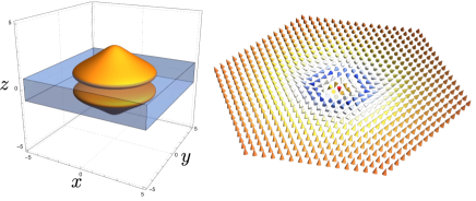
Figure 1: (left) The minimal baryon $f(w)=1/w$. The isosurface of ${\cal B}=1/(50\pi^{2})$ (orange), and the sine-Gordon soliton $\pi/2<\theta<3\pi/2$ (blue). The spatial coordinates are dimensionless with the unit of $m_{\pi}^{-1}$. (right) ${\bm{n}}$ for $k=1$ lump on the soliton.

We now take into account the gauge coupling between ${\bm{n}}$ and $A_{\alpha}$. Since the $U(1)_{\rm EM}$ is generated by $\tau_{3}$, $n_{3}$ is neutral whereas $n_{1}+\text{i}n_{2}\to\text{e}^{-\text{i}\lambda}(n_{1}+\text{i}n_{2})$. Thus the covariant derivative is given by $D_{\alpha}(n_{1}+\text{i}n_{2})=(\partial_{\alpha}-\text{i}eA_{\alpha})(n_{1}+\text{i}n_{2})$. Let $C$ be a closed curve on which $n_{3}=0$, and $D$ be the interior of $C$. The $U(1)_{\rm EM}$ is spontaneously broken around $|n_{1}+\text{i}n_{2}|=1$ where charged pions are condensed. Thus, the closed curve $C$ is a superconducting ring, and there is a persistent current along it. Let us write $n_{1}+\text{i}n_{2}=\text{e}^{i\psi}$ on $C$. The configuration of the gauge field along $C$ is determined by minimizing the gradient energy $|D_{\alpha}(n_{1}+\text{i}n_{2})|^{2}=0$, yielding $\partial_{\alpha}\psi=eA_{\alpha}$. Then, we have a flux (and area) quantization on $D$:

$$BS_{D}=\int_{D}\text{d}^{2}x\,B=\oint_{C}\text{d}x^{i}A_{i}=\frac{1}{e}\oint_{C}\text{d}x^{i}\partial_{i}\psi=\frac{2\pi k}{e}\;\;$$ (28)

with the lump number $k$ on $D$ and the area $S_{D}$ of $D$. This gives a constraint among the lump moduli.

For example, a single ($k=1$) lump is given by $f=b_{0}/w$ with a size and phase moduli $|b_{0}|$ and arg $b_{0}$, respectively, and $n_{3}=(|w|^{2}-|b_{0}|^{2})/(|w|^{2}+|b|^{2})$. Thus, the size of $D$ bounded by $n_{3}=0$ is $|w|=|b_{0}|$, and the flux quantization implies a quantization of the size $|b_{0}|=\sqrt{2/eB}$. Axially symmetric $k$-lumps is given by $f=b_{0}/w^{k}$ and $n_{3}=(|w|^{4}-|b_{0}|^{2})/(|w|^{4}+|b|^{2})$. In this case, we have $|b_{0}|=\sqrt{2k/eB}$.

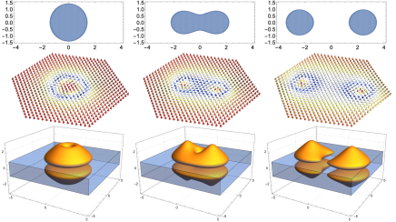
Figure 2: (top) The regions ($S_{D}=4\pi/eB$ with $eB=2$) in the $xy$ plane where $n_{3}\leq 0$ for $k=2$ lumps with $f=\frac{b_{0}}{(w-X)(w+X)}$ with $(b_{0},X)=(2,0),\,(5,2.607),\,(2.595,1.5)$. (middle) ${\bm{n}}$ on the soliton. (bottom) The isosurface of ${\cal B}=1/(15\pi^{2})$.

Finally, we discuss the condition that the lump appears in the ground state but not as an excited one. Inserting eq. (26) into eq. (22), we get 

$$E_{\rm DWSk}=\frac{32\pi f_{\pi}^{2}}{3m_{\pi}}|k|-2\mu_{\textrm{B}}k+e\mu_{\textrm{B}}B|b_{k-1}|^{2}\,.$$ (29)

The condition that the lump is energetically more stable than the uniform state $\bm{n}=(0,0,1)$, or $E<0$, leads to the critical chemical potential for given external parameters, $\mu_{\textrm{B}}$. For $k=1$, the flux quantization condition in eq. (28), or $|b_{0}|=\sqrt{2/eB}$, implies that the last two terms in eq. (29) cancel out, leaving the first term. Since this is positive, single lumps on the domain wall are always excited states, but not spontaneously created. The situation is drastically different for $k\geq 2$. In this case, the energy in eq. (28) is minimized when

$$b_{k-1}=0,\quad{\rm for}\quad k\geq 2.$$ (30)

This condition is consistent with the flux quantization condition eq. (28), unlike the case of $k=1$. For instance, for the $k=2$ axisymmetric lump, $f=b_{0}/w^{2}$ due to eq. (30). Then, the quantization condition (28) imposes $|b_{0}|=2/\sqrt{eB}$. Fig. 2 shows the most general $k=2$ lump configurations $f=\frac{b_{0}}{(w-X)(w+X)}$, in which the $k=2$ axisymmetric lump can be separated into two $k=1$ lumps with keeping the total area and total energy.

The energy of the lump ($k\geq 2$) is negative when eq. (1) holds, yielding a transition from the CSL phase to the domain-wall Skyrmion phase in which lumps are spontaneously created. The phase diagram ¡ is shown in Fig. 3, in which the domain-wall Skyrmion phase meets the CSL and vacuum at the tricritical point ($\mu_{\rm c},3m_{\pi}^{2}/e\sim 0.06{\rm GeV}^{2}\sim 1.0\times 10^{19}{\rm G}$). This point coincides with the instability of CSLs via a charged pion condensation [11], implying that the domain-wall Skyrmion phase is the fate of such an instability.

Apart from the binding energy between a Skyrmion and the domain wall, $\mu_{\textrm{c}}$ is nothing but the nuclear saturation density above which nucleons can be excited, or simply gives the mass of nucleons in this media. It is interesting to point out that $\mu_{\textrm{c}}$ is written thoroughly in terms of only the pion’s decay constant and mass.

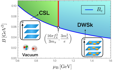
Figure 3: The red and blue lines show $\mu_{\textrm{c}}$ and $B_{\textrm{c}}$, respectively. In the green or blue regions, the ground states are the CSL of $\pi_{0}$ and the domain wall skyrmion (DWSk) phase, respectively.

V Summary

We have reported the existence of the domain-wall Skyrmion phase in QCD matter at finite density with magnetic field. Our results were obtained at the leading ${\cal O}(p^{2})$ order of the ChPT, without a help of higher order corrections such as a Skyrme term. Thus our results are model-independent and robust. The lumps on the domain wall are Skyrmions(baryons) in the bulk, for which one lump corresponds to two baryons. Skyrmions exist in a pair in a Macarons shape with sandwiching the domain wall. The boundary $n_{3}=0$ of the lumps are superconducting rings, yielding the flux quantization condition or the area quantization of the lumps, eq. (28). While single $k=1$ lumps always have positive energy, $k(\geq 2)$ lumps have negative energy in the domain-wall Skyrmion phase. As a byproduct, we have obtained the nuclear saturation density in terms of the pion’s decay constant and mass. The magnetic field $10^{19}{\rm G}$ at the tricritical point is about only 10 times stronger than the ability of current heavy-ion colliders and so it is in scope of future experiments.

An Abrikosov’s vortex lattice was proposed [19] as a possible fate of the charged pion condensation [11]. However they used ${\mathcal{O}}(p^{4})$ order (but not all terms) of the ChPT. In contrast, we have considered the leading ${\mathcal{O}}(p^{2})$ order consistently with all the terms.

Appendix A Derivation of the effective action of a non-Abelian sine-Gordon soliton

Here, we derive the EFT of the non-Abelian sine-Gordon soliton for the both orientational moduli $\phi$ and the translational modulus $Z$, following Ref. [35] in the moduli approximation [36, 37].

We first calculate the effective action coming from eq. (3). Substituting eq. (15) into eq. (3), we get

$$\mathcal{L}_{\textrm{ChPT}}$$

$$=\frac{f_{\pi}^{2}}{2}\left\{\partial_{\alpha}\theta\partial^{\alpha}\theta+|1-u^{2}|^{2}[(\phi^{{\dagger}}\partial_{\alpha}\phi)^{2}+\partial_{\alpha}\phi^{{\dagger}}\partial^{\alpha}\phi]\right\}$$

$$+\frac{e}{2}f_{\pi}^{2}A^{\alpha}|u^{2}-1|^{2}$$

$$\quad\times\left[\phi^{{\dagger}}\tau_{3}\phi\cdot\phi^{{\dagger}}\partial_{\alpha}\phi+\frac{1}{2}(\partial_{\alpha}\phi^{{\dagger}}\tau_{3}\phi-\phi^{{\dagger}}\tau_{3}\partial_{\alpha}\phi)\right]$$

$$-\frac{e^{2}f_{\pi}^{2}}{8}A^{2}|u^{2}-1|^{2}\left[-1+(\phi^{{\dagger}}\tau_{3}\phi)^{2}\right]$$

$$-\frac{f_{\pi}^{2}}{2}(\partial_{z}\theta)^{2}-f_{\pi}^{2}m_{\pi}^{2}(1-\textrm{cos}\theta)\,,$$ (31)

where $x^{\alpha}$ ($\alpha=0,1,2$) are world-volume coordinates. Since $\theta$ depends on $x^{\alpha}$ through $Z(x^{\alpha})$, $\partial_{\alpha}\theta$ becomes

$$\partial_{\alpha}\theta=-\partial_{\alpha}Z\partial_{z}\theta\,,$$ (32)

then $f_{\pi}^{2}\partial_{\alpha}\theta\partial^{\alpha}\theta/2$ can be expressed as

$$\frac{f_{\pi}^{2}}{2}(\partial_{z}\theta)^{2}\partial_{\alpha}Z\partial^{\alpha}Z\,.$$ (33)

Integrating over $z$, the effective action stemming from eq. (3) can be calculated as

$$\int\text{d}z\,\mathcal{L}_{\textrm{ChPT}}$$

$$=4m_{\pi}f_{\pi}^{2}(\partial_{\alpha}Z)^{2}+\frac{16f_{\pi}^{2}}{3m_{\pi}}[(\phi^{{\dagger}}\partial_{\alpha}\phi)^{2}+\partial_{\alpha}\phi^{{\dagger}}\partial^{\alpha}\phi]$$

$$+\frac{16{\text{i}}e}{3m_{\pi}}f_{\pi}^{2}A^{\mu}\left[\phi^{{\dagger}}\tau_{3}\phi\cdot\phi^{{\dagger}}\partial_{\mu}\phi+\frac{1}{2}(\partial_{\mu}\phi^{{\dagger}}\tau_{3}\phi-\phi^{{\dagger}}\tau_{3}\partial_{\mu}\phi)\right]$$

$$-\frac{4e^{2}f_{\pi}^{2}}{3m_{\pi}}A^{2}\left[-1+(\phi^{{\dagger}}\tau_{3}\phi)^{2}\right]-8m_{\pi}f_{\pi}^{2}\,,$$ (34)

where we have used the integrals,

$$\int_{-\infty}^{\infty}\text{d}z\,(\partial_{z}\theta)^{2}=8m_{\pi}\,,$$ (35)

$$\int_{-\infty}^{\infty}\text{d}z\,|1-u^{2}|^{2}=\frac{32}{3m_{\pi}}\,.$$ (36)

The gauge field in the above Lagrangian can be stored in the standard covariant derivative: $D_{\alpha}\phi=(\partial_{\alpha}+\text{i}eA_{\alpha}\tau_{3}/2)\phi$. This comes from the original gauge transformation $\Sigma\to\text{e}^{i\lambda\frac{\tau_{3}}{2}}\Sigma\text{e}^{-i\lambda\frac{\tau_{3}}{2}}$ and $A_{\mu}\to A_{\mu}-\frac{1}{e}\partial_{\mu}\lambda$ with the definition $\Sigma=[{\bm{1}}_{2}+(u^{2}-1)\phi\phi^{{\dagger}}]u^{-1}$ and $\phi\to\text{e}^{\text{i}\frac{\lambda\tau_{3}}{2}}\phi$. Then, eq. (34) is simplified into

$$\int\text{d}z\,\mathcal{L}_{\textrm{ChPT}} =-8f_{\pi}^{2}m_{\pi}+4m_{\pi}f_{\pi}^{2}(\partial_{\alpha}Z)^{2}$$

$$+\frac{16f_{\pi}^{2}}{3m_{\pi}}[(\phi^{{\dagger}}D_{\alpha}\phi)^{2}+D_{\alpha}\phi^{{\dagger}}D^{\alpha}\phi]\,.$$ (37)

The first term is the tension of the non-Abelian sine-Gordon soliton, and the second and third terms are the kinetic terms of $Z$ and $\phi$, respectively.

We next calculate the effective action coming from the WZW term in eq. (6). Due to the eq. (20), the first term can be expressed as $\mu_{\textrm{B}}{\cal B}$. Integration of ${\cal B}$ over $z$ equals twice $q$. Then, we get

$$\int\text{d}z\,\mu_{\textrm{B}}{\cal B}=2\mu_{\textrm{B}}q\,.$$ (38)

The second term in eq. (6) is divided into two terms as follows:

$$\frac{\text{i}e\mu_{\textrm{B}}}{16\pi^{2}}\epsilon^{0ijk}\partial_{i}[A_{j}\mathop{\mathrm{tr}}(\tau_{3}L_{k}+\tau_{3}R_{k})]$$

$$=\frac{\text{i}e\mu_{\textrm{B}}}{16\pi^{2}}\epsilon^{0ijk}\partial_{i}A_{j}\mathop{\mathrm{tr}}(\tau_{3}L_{k}+\tau_{3}R_{k})$$

$$+\frac{\text{i}e\mu_{\textrm{B}}}{16\pi^{2}}\epsilon^{0ijk}A_{j}\mathop{\mathrm{tr}}\tau_{3}(\partial_{i}\Sigma\partial_{k}\Sigma^{{\dagger}}+\partial_{k}\Sigma^{{\dagger}}\partial_{i}\Sigma)\,.$$ (39)

We consider the uniform external magnetic field along the $z$-axis, $\bm{B}=(0,0,B)$. Then, the first term in eq. (39) becomes

$$-\frac{\text{i}e\mu_{\textrm{B}}}{16\pi^{2}}B\mathop{\mathrm{tr}}\tau_{3}(L_{3}+R_{3})\,.$$ (40)

In terms of the projection operator $P\equiv\phi\phi^{{\dagger}}$, $R_{k}$ and $L_{k}$ can be expressed as

$$L_{k}=(1-2P)\text{i}\partial_{k}\theta+(u^{-2}-1)\partial_{k}P+|u^{2}-1|^{2}P\partial_{k}P\,,$$ (41)

$$R_{k}=(1-2P)\text{i}\partial_{k}\theta+(u^{-2}-1)\partial_{k}P+|u^{2}-1|^{2}\partial_{k}P\cdot P\,.$$ (42)

Since $\phi$ does not depend on $z$, the second and third terms in $L_{3}$ and $R_{3}$ vanish. Therefore, eq. (40) becomes

$$-\frac{e\mu_{\textrm{B}}B}{4\pi^{2}}(\phi^{{\dagger}}\tau_{3}\phi)\partial_{3}\theta\,,$$ (43)

and integrating over $z$, we get

$$\int\text{d}z\,\frac{\text{i}e\mu_{\textrm{B}}}{16\pi^{2}}\epsilon^{0ijk}\partial_{i}A_{j}\mathop{\mathrm{tr}}(\tau_{3}L_{k}+\tau_{3}R_{k})=-\frac{e\mu_{\textrm{B}}B}{2\pi}\phi^{{\dagger}}\tau_{3}\phi\,,$$ (44)

where we have used the boundary condition of $\theta$ for a single soliton, $\theta(\infty)-\theta(-\infty)=2\pi$.

We next calculate the second term in eq. (39). Substituting eq. (15) into $\partial_{i}\Sigma\partial_{k}\Sigma^{{\dagger}}$ and $\partial_{k}\Sigma^{{\dagger}}\partial_{i}\Sigma$, these two quantities can be calculated as

$$\partial_{i}\Sigma\partial_{k}\Sigma^{{\dagger}}=\partial_{i}\theta\partial_{k}\theta+[(1-u^{-2})-(u^{2}-u^{-2})P]\text{i}\partial_{i}\theta\partial_{k}P$$

$$-[(1-u^{2})+(u^{2}-u^{-2})P]\text{i}\partial_{k}\theta\partial_{i}P+|1-u^{2}|^{2}\partial_{i}P\partial_{k}P\,,$$ (45)

and

$$\partial_{k}\Sigma^{{\dagger}}\partial_{k}\Sigma=\partial_{i}\theta\partial_{k}\theta+[(1-u^{-2})-(u^{2}-u^{-2})P]\text{i}\partial_{i}\theta\partial_{k}P$$

$$-[(1-u^{2})+(u^{2}-u^{-2})P]\text{i}\partial_{k}\theta\partial_{i}P+|1-u^{2}|^{2}\partial_{k}P\partial_{i}P\,.$$ (46)

Hence, we can represent $\epsilon^{0ijk}\mathop{\mathrm{tr}}(\partial_{i}\Sigma\partial_{k}\Sigma^{{\dagger}}+\partial_{k}\Sigma^{{\dagger}}\partial_{i}\Sigma)$ in terms of $u$ and $\phi$ as follow :

$$\epsilon^{0ijk}\mathop{\mathrm{tr}}\tau_{3}(\partial_{i}\Sigma\partial_{k}\Sigma^{{\dagger}}+\partial_{k}\Sigma^{{\dagger}}\partial_{i}\Sigma)$$

$$=\epsilon^{0ijk}\mathop{\mathrm{tr}}\tau_{3}\{2\text{i}\left[-1+(1+u^{2})P\right](u^{-2}-1)\partial_{i}\theta\partial_{k}P$$

$$\quad+2\text{i}\left[-1+(1+u^{-2})P\right](u^{2}-1)\partial_{i}\theta\partial_{k}P\}$$

$$=2\text{i}|1-u^{2}|^{2}\epsilon^{0ijk}\partial_{i}\theta\mathop{\mathrm{tr}}\tau_{3}\partial_{k}P$$

$$=2\text{i}|1-u^{2}|^{2}\epsilon^{03jk}\partial_{3}\theta\mathop{\mathrm{tr}}\tau_{3}\partial_{k}P\,.$$ (47)

Inserting this expression into the second term in eq (39), it becomes

$$-\frac{e\mu_{\textrm{B}}}{8\pi^{2}}\epsilon^{03jk}|1-u^{2}|^{2}\partial_{3}\theta A_{j}\partial_{k}(\phi^{{\dagger}}\tau_{3}\phi)\,.$$ (48)

Integrating over $z$, we get

$$\int\text{d}z\,\frac{\text{i}e\mu_{\textrm{B}}}{16\pi^{2}}\epsilon^{0ijk}A_{j}\mathop{\mathrm{tr}}\tau_{3}(\partial_{i}\Sigma\partial_{k}\Sigma^{{\dagger}}+\partial_{k}\Sigma^{{\dagger}}\partial_{i}\Sigma)$$

$$=-\frac{e\mu_{\textrm{B}}}{2\pi}\epsilon^{03jk}A_{j}\partial_{k}(\phi^{{\dagger}}\tau_{3}\phi)\,,$$ (49)

where we have used the integral,

$$\int_{-\infty}^{\infty}\text{d}z(u-u^{-1})^{2}\partial_{3}\theta=-4\pi\,.$$ (50)

Summing up eqs. (44) and (49), the effective Lagrangian from the second term in eq. (5) can be calculated as

$$-\frac{e\mu_{\textrm{B}}}{2\pi}\epsilon^{03jk}\partial_{j}(A_{k}\phi^{{\dagger}}\tau_{3}\phi)\,.$$ (51)

Finally, we arrive at the effective Lagrangian of the non-Abelian sine-Gordon soliton under the magnetic field :

$$\mathcal{L}_{\textrm{DW}} \equiv\int\text{d}z\,(\mathcal{L}_{\textrm{ChPT}}+\mathcal{L}_{\textrm{WZW}})$$

$$=8f_{\pi}^{2}m_{\pi}-\frac{e\mu_{\textrm{B}}B}{2\pi}+4m_{\pi}f_{\pi}^{2}(\partial_{\alpha}Z)^{2}$$

$$+\frac{16f_{\pi}^{2}}{3m_{\pi}}[(\phi^{{\dagger}}D_{\alpha}\phi)^{2}+D_{\alpha}\phi^{{\dagger}}D^{\alpha}\phi]$$

$$+2\mu_{\textrm{B}}q+\frac{e\mu_{\textrm{B}}}{2\pi}\epsilon^{03jk}\partial_{j}[A_{k}(1-n_{3})]\,,$$ (52)

which yields eqs. (16), (17) and (18).

Appendix B Correspondence between topological charges in three and two dimensions

Here, we derive the correspondence between the topological charge in three dimensions and two dimensions by using the decomposition of the topological charge density, the Baryon number density, into the sine-Gordon soliton number density and the lump topological charge density. The baryon charge density

$${\cal B}=\frac{-1}{24\pi^{2}}\epsilon^{ijk}\mathop{\mathrm{tr}}(L_{i}L_{j}L_{k}),$$ (53)

can be factorized as

$${\cal B}=-(u-u^{-1})^{2}{\cal W}(z)q(x,y),$$ (54)

where ${\cal W}(w)$ is the domain wall charge density

$${\cal W}(z) \equiv \frac{\partial_{3}\theta}{2\pi}=\frac{m}{\pi\cosh mz},$$ (55)

and the lump topological charge density

$$q(x,y)\equiv-\frac{\text{i}}{2\pi}\epsilon^{ij}\partial_{i}\phi^{{\dagger}}\partial_{j}\phi=\frac{1}{8\pi}\epsilon^{ij}{\bm{n}}\cdot(\partial_{i}{\bm{n}}\times\partial_{j}{\bm{n}}).$$ (56)

The sine-Gordon soliton number and the lump number are given by

$$\int^{\infty}_{-\infty}dz\,{\cal W}=1,\quad\int d^{2}x\,q=k,$$ (57)

respectively. The dressing factor in ${\cal B}$ is given by

$$-(u-u^{-1})^{2}=\frac{16\sinh^{2}mw}{\cosh^{4}mw}.$$ (58)

Thus, the domain wall number density together with the dressing factor determines $z$-dependence of ${\cal B}$

$$-(u-u^{-1})^{2}{\cal W}=\frac{16m\sinh^{2}mw}{\pi\cosh^{5}mw}.$$ (59)

This has two peaks as shown in Fig. 4 and its integration reads

$$-\int^{\infty}_{-\infty}dz\,(u-u^{-1})^{2}{\cal W}=2.$$ (60)

Hence, the $z$ integration of the baryon number density is

$$\int^{\infty}_{-\infty}dz\,{\cal B}=2q(x,y).$$ (61)

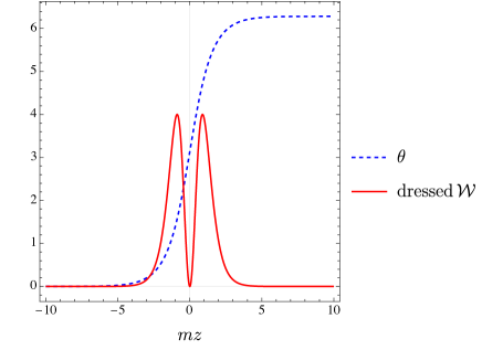
Figure 4: The single sine-Gordon soliton $\theta$ and the dressed domain wall density $-(u-u^{-1})^{2}{\cal W}$.

Appendix C The WZW term for $k$ lumps

Here, we calculate the WZW term. for $k$-lump configuration. Let us take the constant magnetic flux background with

$$A_{i}=-\frac{B}{2}\epsilon_{ij}x^{j},\quad F_{12}=B.$$ (62)

Then, the WZW term includes

$$\frac{e\mu_{\textrm{B}}}{2\pi}\epsilon^{03jk}\partial_{j}[A_{k}(1-n_{3})]$$

$$~{}=-\frac{e\mu_{\textrm{B}}B}{4\pi}\epsilon^{jk}\epsilon_{kl}\partial_{j}\left(x^{l}(1-n_{3})\right)$$

$$~{}=\frac{e\mu_{\textrm{B}}B}{4\pi}\partial_{j}\left(x^{j}(1-n_{3})\right),$$ (63)

where our notation is $\epsilon^{12}=\epsilon_{12}=1$. Next we integrate this over the $xy$ plane

$$\int d^{2}x~{}\frac{e\mu_{\textrm{B}}}{2\pi}\epsilon^{03jk}\partial_{j}[A_{k}(1-n_{3})]$$

$$~{}=\frac{e\mu_{\textrm{B}}B}{4\pi}\int d^{2}x~{}\partial_{j}\left(x^{j}(1-n_{3})\right)$$

$$~{}=\frac{e\mu_{\textrm{B}}B}{4\pi}\oint dS_{j}x^{j}(n_{3}-1).$$ (64)

The lump solution can be easily described by the inhomogeneous coordinate $f\in\mathbb{C}$ by

$$\phi=\frac{1}{\sqrt{1+|f|^{2}}}\left(\begin{array}[]{c}1\\ f\end{array}\right),$$ (67)

providing

$$\phi\phi^{\dagger}=\frac{1}{1+|f|^{2}}\left(\begin{array}[]{cc}1&\bar{f}\\ f&|f|^{2}\end{array}\right).$$ (70)

Then, the equation of motion reduces to

$$\partial_{\bar{w}}f=0,$$ (71)

with $w\equiv x+iy$. Hence $f$ can be an arbitrary meromorphic function

$$f(w)=\frac{b_{k-1}w^{k-1}+\cdots+b_{1}w+b_{0}}{w^{k}+a_{k-1}w^{k-1}+\cdots+a_{1}w+a_{0}}.$$ (72)

The highest power $k$ is the lump charge. The $n_{3}$ component for the $k$ lumps is given by

$$n_{1} = \phi^{\dagger}\tau_{1}\phi=\frac{f+\bar{f}}{1+|f|^{2}}\,,$$ (73)

$$n_{2} = \phi^{\dagger}\tau_{2}\phi=\frac{-i(f-\bar{f})}{1+|f|^{2}}\,,$$ (74)

$$n_{3} = \phi^{\dagger}\tau_{3}\phi=\frac{1-|f|^{2}}{1+|f|^{2}}.$$ (75)

We have $n_{3}=1$ for zeros of $f$, whereas $n_{3}=-1$ for poles of $f$. In order to evaluate the WZW term, it is enough for us to know the asymptotic behavior

$$n_{3}-1\to\frac{r^{2}-|b_{k-1}|^{2}}{r^{2}+|b_{k-1}|^{2}}-1=\frac{-2|b_{k-1}|^{2}}{r^{2}+|b_{k-1}|^{2}}.$$ (76)

Hence, we get

$$\frac{e\mu_{\textrm{B}}B}{4\pi}\oint dS_{j}x^{j}(n_{3}-1)$$

$$~{}=\frac{e\mu_{\textrm{B}}B}{4\pi}\lim_{r\to\infty}\int^{2\pi}_{0}d\theta~{}r^{2}\frac{-2|b_{k-1}|^{2}}{r^{2}+|b_{k-1}|^{2}}$$

$$~{}=-e\mu_{\textrm{B}}B|b_{k-1}|^{2}.$$ (77)

Thus, this term contributes to the energy

$$E\supset e\mu_{\textrm{B}}B|b_{k-1}|^{2}.$$ (78)

This implies that $b_{k-1}=0$ is energetically favored.

References

- Scherer and Schindler [2012] S. Scherer and M. R. Schindler, A Primer for Chiral Perturbation Theory, Vol. 830 (2012).
- Bogner et al. [2010] S. K. Bogner, R. J. Furnstahl, and A. Schwenk, From low-momentum interactions to nuclear structure, Prog. Part. Nucl. Phys. 65, 94 (2010), arXiv:0912.3688 [nucl-th] .
- Skyrme [1962] T. H. R. Skyrme, A Unified Field Theory of Mesons and Baryons, Nucl. Phys. 31, 556 (1962).
- Witten [1983a] E. Witten, Current Algebra, Baryons, and Quark Confinement, Nucl. Phys. B 223, 433 (1983a).
- Son and Stephanov [2008] D. T. Son and M. A. Stephanov, Axial anomaly and magnetism of nuclear and quark matter, Phys. Rev. D 77, 014021 (2008), arXiv:0710.1084 [hep-ph] .
- Son and Zhitnitsky [2004] D. T. Son and A. R. Zhitnitsky, Quantum anomalies in dense matter, Phys. Rev. D 70, 074018 (2004), arXiv:hep-ph/0405216 .
- Goldstone and Wilczek [1981] J. Goldstone and F. Wilczek, Fractional Quantum Numbers on Solitons, Phys. Rev. Lett. 47, 986 (1981).
- Witten [1983b] E. Witten, Global Aspects of Current Algebra, Nucl. Phys. B 223, 422 (1983b).
- Eto et al. [2013] M. Eto, K. Hashimoto, and T. Hatsuda, Ferromagnetic neutron stars: axial anomaly, dense neutron matter, and pionic wall, Phys. Rev. D 88, 081701 (2013), arXiv:1209.4814 [hep-ph] .
- Brauner and Yamamoto [2017] T. Brauner and N. Yamamoto, Chiral Soliton Lattice and Charged Pion Condensation in Strong Magnetic Fields, JHEP 04, 132, arXiv:1609.05213 [hep-ph] .
- Brauner and Kadam [2017a] T. Brauner and S. V. Kadam, Anomalous low-temperature thermodynamics of QCD in strong magnetic fields, JHEP 11, 103, arXiv:1706.04514 [hep-ph] .
- Brauner and Kadam [2017b] T. Brauner and S. Kadam, Anomalous electrodynamics of neutral pion matter in strong magnetic fields, JHEP 03, 015, arXiv:1701.06793 [hep-ph] .
- Brauner et al. [2021] T. Brauner, H. Kolešová, and N. Yamamoto, Chiral soliton lattice phase in warm QCD, Phys. Lett. B 823, 136767 (2021), arXiv:2108.10044 [hep-ph] .
- Brauner and Kolešová [2023] T. Brauner and H. Kolešová, Chiral soliton lattice at next-to-leading order, (2023), arXiv:2302.06902 [hep-ph] .
- Huang et al. [2018] X.-G. Huang, K. Nishimura, and N. Yamamoto, Anomalous effects of dense matter under rotation, JHEP 02, 069, arXiv:1711.02190 [hep-ph] .
- Nishimura and Yamamoto [2020] K. Nishimura and N. Yamamoto, Topological term, QCD anomaly, and the chiral soliton lattice in rotating baryonic matter, JHEP 07 (07), 196, arXiv:2003.13945 [hep-ph] .
- Eto et al. [2022] M. Eto, K. Nishimura, and M. Nitta, Phases of rotating baryonic matter: non-Abelian chiral soliton lattices, antiferro-isospin chains, and ferri/ferromagnetic magnetization, JHEP 08, 305, arXiv:2112.01381 [hep-ph] .
- Chen et al. [2021] H.-L. Chen, X.-G. Huang, and J. Liao, QCD phase structure under rotation, Lect. Notes Phys. 987, 349 (2021), arXiv:2108.00586 [hep-ph] .
- Evans and Schmitt [2022] G. W. Evans and A. Schmitt, Chiral anomaly induces superconducting baryon crystal, JHEP 09, 192, arXiv:2206.01227 [hep-th] .
- Kawaguchi et al. [2019] M. Kawaguchi, Y.-L. Ma, and S. Matsuzaki, Chiral soliton lattice effect on baryonic matter from a skyrmion crystal model, Phys. Rev. C 100, 025207 (2019), arXiv:1810.12880 [nucl-th] .
- Chen et al. [2022] S. Chen, K. Fukushima, and Z. Qiu, Skyrmions in a magnetic field and 0 domain wall formation in dense nuclear matter, Phys. Rev. D 105, L011502 (2022), arXiv:2104.11482 [hep-ph] .
- Chen et al. [2023] S. Chen, K. Fukushima, and Z. Qiu, Magnetic enhancement of baryon confinement modeled via a deformed Skyrmion, (2023), arXiv:2303.04692 [hep-th] .
- Eto and Nitta [2022] M. Eto and M. Nitta, Quantum nucleation of topological solitons, JHEP 09, 077, arXiv:2207.00211 [hep-th] .
- Higaki et al. [2022] T. Higaki, K. Kamada, and K. Nishimura, Formation of a chiral soliton lattice, Phys. Rev. D 106, 096022 (2022), arXiv:2207.00212 [hep-th] .
- Yamada and Yamamoto [2021] A. Yamada and N. Yamamoto, Floquet vacuum engineering: Laser-driven chiral soliton lattice in the QCD vacuum, Phys. Rev. D 104, 054041 (2021), arXiv:2107.07074 [hep-ph] .
- Brauner et al. [2019a] T. Brauner, G. Filios, and H. Kolešová, Chiral soliton lattice in QCD-like theories, JHEP 12, 029, arXiv:1905.11409 [hep-ph] .
- Brauner et al. [2019b] T. Brauner, G. Filios, and H. Kolešová, Anomaly-Induced Inhomogeneous Phase in Quark Matter without the Sign Problem, Phys. Rev. Lett. 123, 012001 (2019b), arXiv:1902.07522 [hep-ph] .
- Togawa et al. [2016] Y. Togawa, Y. Kousaka, K. Inoue, and J.-i. Kishine, Symmetry, structure, and dynamics of monoaxial chiral magnets, Journal of the Physical Society of Japan 85, 112001 (2016).
- Polyakov and Belavin [1975] A. M. Polyakov and A. A. Belavin, Metastable States of Two-Dimensional Isotropic Ferromagnets, JETP Lett. 22, 245 (1975).
- Nitta [2013a] M. Nitta, Correspondence between Skyrmions in 2+1 and 3+1 Dimensions, Phys. Rev. D 87, 025013 (2013a), arXiv:1210.2233 [hep-th] .
- Nitta [2013b] M. Nitta, Matryoshka Skyrmions, Nucl. Phys. B 872, 62 (2013b), arXiv:1211.4916 [hep-th] .
- Gudnason and Nitta [2014a] S. B. Gudnason and M. Nitta, Domain wall Skyrmions, Phys. Rev. D 89, 085022 (2014a), arXiv:1403.1245 [hep-th] .
- Gudnason and Nitta [2014b] S. B. Gudnason and M. Nitta, Incarnations of Skyrmions, Phys. Rev. D 90, 085007 (2014b), arXiv:1407.7210 [hep-th] .
- Nitta [2015] M. Nitta, Non-Abelian Sine-Gordon Solitons, Nucl. Phys. B 895, 288 (2015), arXiv:1412.8276 [hep-th] .
- Eto and Nitta [2015] M. Eto and M. Nitta, Non-Abelian Sine-Gordon Solitons: Correspondence between Skyrmions and Lumps, Phys. Rev. D 91, 085044 (2015), arXiv:1501.07038 [hep-th] .
- Manton [1982] N. S. Manton, A Remark on the Scattering of BPS Monopoles, Phys. Lett. B 110, 54 (1982).
- Eto et al. [2006] M. Eto, Y. Isozumi, M. Nitta, K. Ohashi, and N. Sakai, Manifestly supersymmetric effective Lagrangians on BPS solitons, Phys. Rev. D 73, 125008 (2006), arXiv:hep-th/0602289 .
- Note [1] See Appendix A for a derivation of the domain-wall EFT.
- Note [2] See Appendix B for a derivation.
- Note [3] Exactly speaking this corresponds to a parameter region that with keeping .
- Note [4] This situation is similar to magnetic skyrmions in chiral magnets, in which case the DM interaction plays such a role.
- Nitta [2022] M. Nitta, Relations among topological solitons, Phys. Rev. D 105, 105006 (2022), arXiv:2202.03929 [hep-th] .
- Note [5] Two-dimensional version of domain-wall skyrmions were also earlier found in field theory [45, 46, 47] and studied experimentally and theoretically in chiral magnets [48, 49, 50, 51, 52, 53] (see also [54]).
- Note [6] See Appendix C for a derivation.
- Nitta [2012] M. Nitta, Josephson vortices and the Atiyah-Manton construction, Phys. Rev. D 86, 125004 (2012), arXiv:1207.6958 [hep-th] .
- Kobayashi and Nitta [2013] M. Kobayashi and M. Nitta, Sine-Gordon kinks on a domain wall ring, Phys. Rev. D 87, 085003 (2013), arXiv:1302.0989 [hep-th] .
- Jennings and Sutcliffe [2013] P. Jennings and P. Sutcliffe, The dynamics of domain wall Skyrmions, J. Phys. A 46, 465401 (2013), arXiv:1305.2869 [hep-th] .
- Cheng et al. [2019] R. Cheng, M. Li, A. Sapkota, A. Rai, A. Pokhrel, T. Mewes, C. Mewes, D. Xiao, M. De Graef, and V. Sokalski, Magnetic domain wall skyrmions, Phys. Rev. B 99, 184412 (2019).
- Lepadatu [2020] S. Lepadatu, Emergence of transient domain wall skyrmions after ultrafast demagnetization, Phys. Rev. B 102, 094402 (2020).
- Kuchkin et al. [2020] V. M. Kuchkin, B. Barton-Singer, F. N. Rybakov, S. Blügel, B. J. Schroers, and N. S. Kiselev, Magnetic skyrmions, chiral kinks and holomorphic functions, Phys. Rev. B 102, 144422 (2020), arXiv:2007.06260 [cond-mat.str-el] .
- T.Nagase et al. [2021] T.Nagase, Y.-G. So, H. Yasui, T. Ishida, H. K. Yoshida, Y. Tanaka, K. Saitoh, N. Ikarashi, Y. Kawaguchi, M. Kuwahara, and M. Nagao, Observation of domain wall bimerons in chiral magnets, Nature Commun. 12, 3490 (2021), arXiv:2004.06976 [cond-mat.mtrl-sci] .
- Yang et al. [2021] K. Yang, K. Nagase, and Y. Hirayama et.al., Wigner solids of domain wall skyrmions, Nat Commun 12, 6006 (2021).
- Ross and Nitta [2023] C. Ross and M. Nitta, Domain-wall skyrmions in chiral magnets, Phys. Rev. B 107, 024422 (2023), arXiv:2205.11417 [cond-mat.mes-hall] .
- Kim and Tserkovnyak [2017] S. K. Kim and Y. Tserkovnyak, Magnetic Domain Walls as Hosts of Spin Superfluids and Generators of Skyrmions, Phys. Rev. Lett. 119, 047202 (2017), arXiv:1701.08273 [cond-mat.mes-hall] .