The indication for ⁴⁰K geo-antineutrino flux with Borexino phase-III data

Abstract

Abstract $-$ We provide the indication of high flux of ⁴⁰K geo-antineutrino and geo-neutrino (⁴⁰K-geo-($\bar{\nu}+\nu$)) with Borexino Phase III data. This result was obtained by introducing a new source of single events, namely ⁴⁰K-geo-($\bar{\nu}+\nu$) scattering on electrons, in multivariate fit analysis of Borexino Phase III data. Simultaneously we obtained the count rates of events from ⁷Be, $pep$ and CNO solar neutrinos. These count rates are consistent with the prediction of the Low metallicity Sun model SSM B16-AGSS09. MC pseudo-experiments showed that the case of High metallicity Sun and absence of ⁴⁰K-geo-($\bar{\nu}+\nu$) can not imitate the result of multivariate fit analysis of Borexino Phase III data with introducing ⁴⁰K-geo-($\bar{\nu}+\nu$) events. We also provide arguments for the high abundance of potassium in the Earth.

Keywords: Borexino detector, potassium geo-antineutrino, Low metallicity Sun, Earth intrinsic heat.

1 Introduction

The Borexino collaboration reported in [1] an improved measurement of the Carbon-Nitrogen-Oxygen (CNO) solar neutrino interaction rate at Earth obtained with the complete Borexino Phase-III dataset. The measured rate, $R_{\rm CNO}=6.7^{+2.0}_{-0.8}$ cpd/100t (counts/(day $\times$ 100 tonnes)).

The main idea of this article is to see what could happen if we introduce in analysis the new source of single events from ⁴⁰K geo-antineutrino and neutrino (⁴⁰K-geo-($\bar{\nu}+\nu$)) scattering on electrons. Such source was proposed in [2, 3] and such analysis were done in [4] by using Borexino phase II dataset from [5] and in [6] by using Borexino phase III dataset.

We will use in this paper the Phase-III dataset which is different from Phase-II dataset [5]. The Phase-III dataset was taken when the radiopurity and thermal stability of the detector was maximal, i. e. between January 2017 and October 2021. The Phase-II dataset was taken from July 2016 until February 2020. The Phase-III statistics is higher than the Phase-II statistics on about 30%.

We hope that the obtained result will attract the attention of the scientific community to an alternative interpretation of the Borexino data and encourage further research of solar neutrino and potassium geo-antineutrino fluxes.

2 Energy spectrum of recoil electrons from ⁴⁰K-geo-($\bar{\nu}+\nu$)

⁴⁰K abundance in natural mixture of K isotopes is 0.0117%. It decays with $T_{1/2}=1.248\cdot 10^{9}$ y through two modes: to ⁴⁰Ca with efficiency 89.28% emitting $\bar{\nu_{e}}$ with maximal energy 1.311 keV and to ⁴⁰Ar emitting one of two possible mono-energetic $\nu_{e}$-s with energies 43.5 keV (10.67%) and 1.504 keV ($\sim$0.05%). Decay scheme of ⁴⁰K can be found in [7]. Low energy neutrinos cannot be detected but high energy ones can be seen in large volume detector as a small addition to antineutrino’s effect.

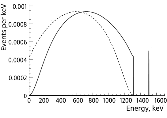
Figure 1: ⁴⁰K antineutrinos and neutrinos spectra $-$ solid line. The spectra are normalized to the probablity of emission in decay: 0.8928 for $\bar{\nu_{e}}$-s and 0.0005 for $\nu_{e}$-s. Energy spectrum of electrons emitted in ⁴⁰K decay $-$ dashed line.

Figure 1 demonstrates the total beta, antineutrino and neutrino energy spectra for ⁴⁰K decay. The antineutrino spectrum was calculated using the beta one taken in [7]. The beta spectrum is the same as was measured in [8] and calculated in [9].

Figure 2: The energy spectrum of recoil electrons from ⁴⁰K-geo-($\bar{\nu}+\nu$). The pedestal at higher energies corresponds to neutrinos. The total counting rate of recoil electrons for this spectrum is 2.18 cpd/100t.

In Figure 2 one can see the calculated energy spectrum of recoil electrons for ⁴⁰K-geo-($\bar{\nu}+\nu$) that follows from the spectrum shape shown in Figure 1. The pedestal at higher energies corresponds to 1.5-MeV neutrinos. The total counting rate of recoil electrons for the spectrum shown in Figure 2 is equal to 2.18 cpd/100t that corresponds to potassium abundance 1.0% of the Earth mass in the case of uniform distribution of potassium in the Earth.

The energy spectrum normalized to unit is the probability density function and we will use below the notation PDF for such normalized spectrum.

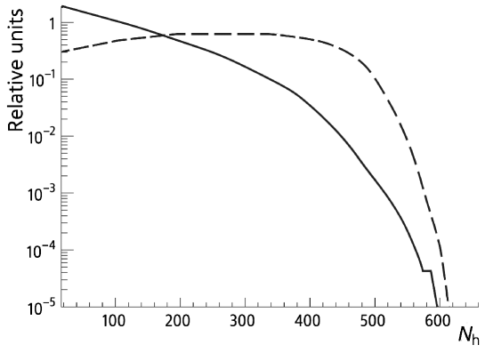
Figure 3: Recoil electron spectrum from ⁴⁰K-geo-($\bar{\nu}$ + $\nu$) transferred to $N_{h}$ (numder of hit PMTs) scale according to the algorithm from [10]$-$ solid line. Energy spectrum of electrons emitted in ⁴⁰K decay $-$ dashed line.

We will use PDFs in multivariate fit analysis (MF) as a function of number of hit PMTs $N_{h}$ following the Borexino Collaboration. The calculated recoil electron energy spectrum from ⁴⁰K-geo-($\bar{\nu}+\nu$) was transferred from the energy scale to $N_{h}$ scale using the algorithm described in [10]. In Figure 3 one can find ⁴⁰K-geo-($\bar{\nu}+\nu$) PDF used in the MF analysis. ⁴⁰K $\beta$ spectrum PDF is also shown here for comparison.

To prove that we correctly perform the calculation of ⁴⁰K-geo-($\bar{\nu}$ + $\nu$) PDF, one can compare our ⁷Be PDF and the one taken from Borexino plot [5] shown in Figure 4.

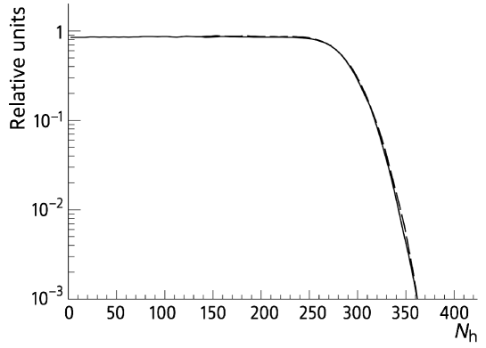
Figure 4: PDF of recoil electron spectrum from ⁷Be neutrinos transferred to $N_{h}$ (numder of hit PMTs) scale according to the algorithm from [10]. Solid line $-$ our calculation, dashed line $-$ [5].

3 Energy spectrum of recoil electrons from CNO-$\nu$

The CNO-$\nu$ spectrum consists of three components: the ¹³N, ¹⁵O and ¹⁷F neutrino spectra. The shape of these spectra is well known because the transitions are allowed and can be easily calculated. However, the fluxes depend on the solar model, and many flux predictions exist. In Table 1 we can see a number of flux predictions for ¹³N, ¹⁵O and ¹⁷F according to different models.

Table 1: Neutrino fluxes produced in the Sun by nuclei ¹³N, ¹⁵O and ¹⁷F in units cm^-2 s^-1.

Model	13N$\times 10^{8}$	15O$\times 10^{8}$	17F$\times 10^{6}$
B16 [11]	5.03	1.34	$<$8.5
GS98 [12]	2.78	2.05	5.29
AGSS09 [12]	2.04	1.44	3.26
Caffau11 [13]	2.801	2.123	4.648
used in Borexino [14]	2.78	2.05	5.29

We have calculated neutrino spectra from ¹³N, ¹⁵O and ¹⁷F ourselves in the moment of production inside the Sun. These calculated spectra undergo oscillations according to the MSW-mechanism [15]. As a result each spectrum split in two: the electron neutrino spectrum and $\nu_{\mu}$ + $\nu_{\tau}$ spectrum. For each one we calculated a recoil electron spectrum and composed them in one. The sum of three CNO components appear similar to the CNO spectrum used in the Borexino analysis but not exactly. So, we decided to use in our analysis the CNO spectrum digitized from the plot of the Borexino publication. We can see in Table 1 that spectrum used in the Borexino analysis corresponds to High metallicity Sun model GS98. Later we are going to make the analysis using CNO spectrum corresponding to Low metallicity Sun model AGSS09, see Table 1.

4 Borexino experimental data multivariate fit analysis

We will use here the dataset digitized from the figure from [1] with suppressed contribution of the cosmogenic ¹¹C background. The histogram of the number of events of Phase III $N$ depending on the number of hit PMTs $N_{h}$ is shown in Table 2.

Table 2: Experimental histogram of the number of events $N$ of Phase III depending on the number of hit PMTs $N_{h}$ from [1]. Bin centers are shown in columns labeled as $N_{h}$. Events were collected over 871.31 days in 71.3 t.

$N_{h}$	$N$	$N_{h}$	$N$	$N_{h}$	$N$	$N_{h}$	$N$	$N_{h}$	$N$	$N_{h}$	$N$	$N_{h}$	$N$	$N_{h}$	$N$	$N_{h}$	$N$
140	1021	230	931	320	167	410	55	500	54	590	34	680	25	770	23	860	40
145	1098	235	834	325	123	415	68	505	46	595	34	685	22	775	35	865	36
150	1251	240	725	330	110	420	43	510	53	600	31	690	22	780	26	870	37
155	1573	245	663	335	105	425	56	515	50	605	31	695	20	785	34	875	39
160	1801	250	677	340	76	430	71	520	50	610	26	700	15	790	31	880	35
165	2097	255	602	345	712	435	62	525	39	615	25	705	20	795	33	885	28
170	2614	260	797	350	71	440	43	530	44	620	31	710	20	800	34	890	35
175	3044	265	555	355	60	445	46	535	47	625	21	715	14	805	37	895	32
180	3341	270	562	360	55	450	65	540	36	630	21	720	19	810	42	900	26
185	3471	275	479	365	59	455	57	545	36	635	30	725	24	815	26	905	33
190	3341	280	425	370	56	460	45	550	26	640	28	730	24	820	36	910	25
195	3285	285	406	375	51	465	62	555	35	645	25	735	24	825	38	915	22
200	2869	290	365	380	44	470	71	560	46	650	16	740	19	830	38	920	27
205	2443	295	316	385	59	475	70	565	35	655	25	745	24	835	29	925	22
210	2151	300	265	390	49	480	58	570	39	660	17	750	29	840	39	930	20
215	1741	305	233	395	46	485	52	575	35	665	25	755	22	845	33	935	13
220	1368	310	191	400	51	490	40	580	24	670	25	760	24	850	44	940	19
225	1160	315	198	405	56	495	57	585	37	675	23	765	32	855	52	945	11

We have calculated PDFs for most of the components used in the Borexino analysis and used them in our multivariate fit (MF) analysis (⁷Be, $pep$, ¹¹C, ²¹⁰Bi, ⁸⁵Kr and CNO). Four components were digitized from [5], they are: ²¹⁰Po alpha-peak, ⁸B and two backgrounds caused by external gammas from ²⁰⁸Tl and the summed spectrum of ²¹⁴Bi and ⁴⁰K gammas.

The $\chi^{2}$ function was used to estimate the goodness of our fit:

$$\chi^{2}=\sum_{i=1}^{162}\frac{(N_{i}-\sum_{k=1}^{10}w_{k}\cdot f_{k,i})^{2}}{\sigma^{2}_{i}},$$ (1)

where $N_{i}$ is the experimental value of counting rate of the Borexino detector events in the $i$-th bin of the number of hitted PMTs, $w_{k}=R_{k}\cdot 0.713\cdot t_{meas}-$ the weight for the PDF of the $k$-th component with $R_{k}-$ the total counting rate of the $k$-th component in cpd/100t, 0.713 $-$ the ratio of 71.3 t and 100 t and $t_{meas}-$ the measurement time in days, $f_{k,i}-$ the PDF of the $k$-th component and $\sigma_{i}$ is experimental uncertainty. We used a standard tool for analysis, ROOT 6.22/08, to find the set of parameters $R_{k}\pm\Delta R_{k}$ which minimizes $\chi^{2}$. The $\Delta R_{k}$ corresponds to the confidence level of $68\%$ in ROOT 6.22/08. To check the results of ROOT we used also another minimization code.

Table 3: Total counting rates and $\chi^{2}$ obtained without (column 1 and 1a) and with (column 2 and 2a) the ⁴⁰K-geo-($\bar{\nu}+\nu$) component of the fit, cpd/100t. Comparison of the experimental results of solar neurtino counting rates from MFs and theoretical predictions for High metallicity (column 3) and Low metallicity (column 4) [10], cpd/100t.

	Mod.1,exp.	Mod.1,cpd range	Mod.2,exp.	Mod.2,cpd range	B16CS98	B16AGSS09
					HZ	LZ
	1	1 a	2	2 a	3	4
7Be	48.4 $\pm$ 0.9	46$\div$49	46.0 $\pm$ 0.84	42$\div$49	47.9 $\pm$ 2.8	43.7 $\pm$ 2.5
$pep$	2.7	2.7	2.78 $\pm$ 0.07	2.7$\div$2.78	2.74 $\pm$ 0.04	2.78 $\pm$ 0.04
CNO	6.5 $\pm$ 0.7	4.5$\div$8	3.67 $\pm$ 0.73	3.5$\div$20	4.92 $\pm$ 0.55	3.52 $\pm$ 0.37
11C	1.7$\pm$ 0.1	1.35$\div$2	1.83 $\pm$ 0.07	1.4$\div$2
210Po	41.5$\pm$0.4	40$\div$46	41.1$\pm$ 0.08	35$\div$45
210Bi	11.8	9.8$\div$11.8	11.0 $\pm$ 0.23	10.7$\div$11
85Kr	8.5	3.5$\div$8.5	8.5 $\pm$ 0.24	3.5$\div$8.5
208Tl	4.76$\pm$ 0.2	4.3$\div$5	4.76	4.7/6
214Bi	1.8$\pm$ 0.3	1.7$\div$2	1.79	1.79
40Kgeo	0.0	0.0	11 $\pm$ 0.6	0$\div$11
$\chi^{2}_{1},\chi^{2}_{2}$	199.5		173.5

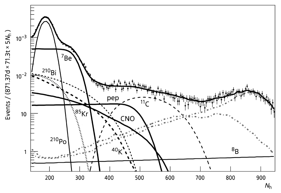
Figure 5: Counting rate of recoil electrons and alphas in Borexino detector in 5 hits bin versus number of hit PMTs. The values of points with errors from [1] are given in Table 2. The curves are the contributions of different components of the fit and the sum of all components obtained by the MF analysis. Dark black dashed curve is contribution of ⁴⁰K-geo-($\bar{\nu}+\nu$) events. The obtained total counting rates for components of the fit are presented in the second column of the Table 3.

The PDF for ⁴⁰K-geo-($\bar{\nu}$ + $\nu$) was added to the analysis. So, in total we have 10 PDFs to fit: ⁷Be, $pep$, ¹¹C, ²¹⁰Po, ²¹⁰Bi, ⁸⁵Kr, external backgrounds 1 and 2, CNO and ⁴⁰K-geo-($\bar{\nu}$ + $\nu$). ⁸B was fixed.

At the first stage we made the fit of Borexino dataset by minimization of $\chi^{2}$ from (1) using our calculated PDFs for the components but ⁴⁰K-geo-($\bar{\nu}$ + $\nu$) was set to zero. We used the energy range from 140 to 945 hits following the Borexino analysis. The experimental dataset was described with a sum of 8 variable components. The $pep$ was fix and other parameters were constrained as column 1a of Table 3 shows. The upper limits of constraints for ²¹⁰Bi and ⁸⁵Kr we took from Borexino measurements of the upper limits of ²¹⁰Bi and ⁸⁵Kr concentrations in scintillator. As a result we obtained total counting rates that are on the first column of Table 3. We can observe the similarity of the obtained values of the parameters to the parameters presented by Borexino Collaboration in [1, 10] and references inside them. The obtained values of $R$(⁷Be), $R(pep)$, $R$(CNO) support the Sun model of High metallicity. Theoretical predictions for High metallicity Sun are shown in column 3 of Table 3.

The PDF of ⁴⁰K-geo-($\bar{\nu}+\nu$) was added at the second stage of the analysis. We made 8 parameters free (constrained) and external backgrounds 1 and 2 were fixed as column 2a of Table 3 shows.

The result of this fit is shown in Figure 5 and obtained total counting rates are in the second column of Table 3. We obtained the value of $R(^{40}$K-geo-$(\bar{\nu}+\nu))=11\pm 0.6$ cpd/100t. The fit found also the reasonable values of total counting rates for all components. The obtained values in second stage of ananlysis of $R$(⁷Be), $R(pep)$, $R$(CNO) support the Sun model of Low metallicity in contrary to the first stage analysis. Theoretical predictions for Low metallicity Sun are shown in column 4 of Table 3. We note here that $\chi^{2}_{2}$ values obtained at the second stage is lower (better) than obtained at the first stage $\chi^{2}_{1}$. The $\chi^{2}_{1}$ and $\chi^{2}_{2}$ values are shown in last row of Table 3. This means that Low metallicity Sun and high abundance of potassiun in the Earth is more realistic than High metallicity Sun and low abundace of potassium in the Earth.

The inclusion of the scattering of ⁴⁰K-geo-($\bar{\nu}+\nu$) on electrons in the analysis mainly reduces the number of events from ⁷Be and CNO. But the number of events from $pep$ becomes a little higher.

Note that the error for the counting rate of ⁴⁰K-geo-$(\bar{\nu}+\nu)$ events given in column 2 of the Table 3 characterizes the minimum of the function $\chi^{2}$ and is not an experimental error in measuring the value of $R(^{40}$K-geo-$(\bar{\nu}+\nu))$.

5 Simulation of the experiment

We performed MC simulated experiments to understand the influence of the finite sample of data, the parameter constraints and the other conditions of the fit on reconstructed results. The MC simulated experiments help also to understand the possibilities of a next generation Borexino-type detector to measure the ⁴⁰K-geo-$(\bar{\nu}+\nu)$ flux accurately.

We took a set of PDFs with certain fixed counting rates and simulated the Borexino-like spectrum of single events many times via the MC method. Each time we had a new finite sample of Borexino-like data. We reconstructed the values of counting rates using the procedure (1) described above for each sample and, as a result, obtained probability distributions of the reconstructed counting rates and $\chi^{2}_{1}$ and $\chi^{2}_{2}$. We obtained wide non-symmetric distributions with their mean values different from the values fixed in MC mainly for components with low counting rates $R(^{40}$K-geo) and $R$(CNO). The main reason for this is the effect of statistical fluctuations of components with high counting rates. These fluctuations affect the reconstructed counting rates of components with low counting rates. The value of this effect depends on statistics. Therefore, we found that the reconstructed counting rates in the Borexino-like data samples obtained using this procedure can have systematic biases relative to their true values.

Below we will give an examples of our pseudo-experiments. We have two sets of components after our MFs of the experimental Borexino data sample. One set is in the first column of Table 3 and another set is in the second column of Table 3. The main difference is the reconstructed $R(^{40}$K-geo-($\bar{\nu}+\nu)$), $R(^{7}$Be) and $R$(CNO) rates.

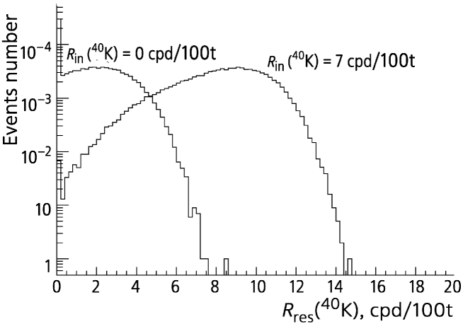
Figure 6: Reconstructed counting rate $R_{\rm{res}}(^{40}$K-geo-$(\bar{\nu}+\nu))$ distributions for $10^{5}$ pseudo-experiments. The curve labled $R_{\rm{in}}(^{40}$K) = 0 cpd/100t is the result of pseudo-experiments with parameters from column 1 of the Table 3. The mean value of this distribution is $R_{\rm{res}}(^{40}$K-geo-$(\bar{\nu}+\nu))$ = 1.67 cpd/100t and $\sigma=1.53$ cpd/100t. The curve labled $R_{\rm{in}}(^{40}$K) = 7 cpd/100t is the result of pseudo-experiments with parameters from column 2 of the Table 3 but with $R(^{40}$K-geo-$(\bar{\nu}+\nu))$ = 7 cpd/100t.

At first we chose for our example of pseudo-experiments the parameters from first column of Table 3. But when we reconstructed the parameters, we included the PDF of $R(^{40}$K-geo-($\bar{\nu}+\nu)$) in procedure (1) and applied the constraints as column 2a of Table 3 shows. The idea was to test whether reality without potassium could simulate our result with $R(^{40}$K-geo-$(\bar{\nu}+\nu))=11$ cpd/100t. The curve labled a $R_{\rm{in}}(^{40}$K) = 0 cpd/100t on Figure 6 shows the distribution of reconstructed $R_{\rm{res}}(^{40}$K-geo-$(\bar{\nu}+\nu))$ for $10^{5}$ pseudo-experiments. We see that probability to observe $R(^{40}$K-geo-$(\bar{\nu}+\nu))>7$ cpd/100t is less than $10^{-5}$.

Then we chose for our another example of pseudo-experiments the parameters from second column of Table 3. Knowing about the existence of systematic biases, we took for MC simulation of data samples the counting rate $R(^{40}$K-geo-($\bar{\nu}+\nu)$) = 7 cpd/100t instead of the value in the second column of Table 3. We applied the constraints as column 2a of Table 3 shows but $R(^{40}$K-geo-$(\bar{\nu}+\nu))$ was free. The curve labled $R_{\rm{in}}(^{40}$K) = 7 cpd/100t on Figure 6 shows the distribution of reconstructed $R_{\rm{res}}(^{40}$K-geo-$(\bar{\nu}+\nu))$ for $10^{5}$ pseudo-experiments. We see that our result $R(^{40}$K-geo-$(\bar{\nu}+\nu))=11$ cpd/100t has the high probability in this case. We see also a systematic bias and the need a big statistic to measure the potassium abundance more accurately. We constructed the $\chi^{2}_{1}$ and $\chi^{2}_{2}$ distributions obtained as a result of approximation these MC data samples by the sets of single event sources without of $R(^{40}$K-geo-$(\bar{\nu}+\nu))$ and with of $R(^{40}$K-geo-$(\bar{\nu}+\nu))$ correspondently . The distributions has the gaussian form with $\bar{\chi}^{2}_{1}=184.4\pm 21.17.$ and $\bar{\chi}^{2}_{2}=167.4\pm 19.79.$ The obtained values $\chi^{2}_{1}=199.5$ and $\chi^{2}_{2}=173.5$ for experimental Borexino phase III dataset (see Table 3) is not contradict to these MC values. At first we chose for our example of pseudo-experiments the parameters from first column of Table 3. But when we reconstructed the parameters, we included the PDF of $R(^{40}$K-geo-($\bar{\nu}+\nu)$) in procedure (1) and applied the constraints as column 2a of Table 3 shows. The idea was to test whether reality without potassium could simulate our result with $R(^{40}$K-geo-$(\bar{\nu}+\nu))=11$ cpd/100t. The curve labled a $R_{\rm{in}}(^{40}$K) = 0 cpd/100t on Figure 6 shows the distribution of reconstructed $R_{\rm{res}}(^{40}$K-geo-$(\bar{\nu}+\nu))$ for $10^{5}$ pseudo-experiments. We see that probability to observe $R(^{40}$K-geo-$(\bar{\nu}+\nu))>7$ cpd/100t is less than $10^{-5}$.

Then we chose for our another example of pseudo-experiments the parameters from second column of Table 3. Knowing about the existence of systematic biases, we took for MC simulation of data samples the counting rate $R(^{40}$K-geo-($\bar{\nu}+\nu)$) = 7 cpd/100t instead of the value in the second column of Table 3. We applied the constraints as column 2a of Table 3 shows but $R(^{40}$K-geo-$(\bar{\nu}+\nu))$ was free. The curve labled $R_{\rm{in}}(^{40}$K) = 7 cpd/100t on Figure 6 shows the distribution of reconstructed $R_{\rm{res}}(^{40}$K-geo-$(\bar{\nu}+\nu))$ for $10^{5}$ pseudo-experiments. We see that our result $R(^{40}$K-geo-$(\bar{\nu}+\nu))=11$ cpd/100t has the high probability in this case. We see also a systematic bias and the need a big statistic to measure the potassium abundance more accurately. We constructed the $\chi^{2}_{1}$ and $\chi^{2}_{2}$ distributions obtained as a result of approximation these MC data samples by the sets of single event sources without of $R(^{40}$K-geo-$(\bar{\nu}+\nu))$ and with of $R(^{40}$K-geo-$(\bar{\nu}+\nu))$ correspondently . The distributions has the gaussian form with $\bar{\chi}^{2}_{1}=184.4\pm 21.17.$ and $\bar{\chi}^{2}_{2}=167.4\pm 19.79.$ The obtained values $\chi^{2}_{1}=199.5$ and $\chi^{2}_{2}=173.5$ for experimental Borexino phase III dataset (see Table 3) is not contradict to these MC values.

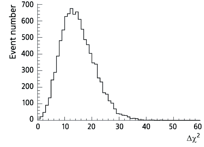
Figure 7: Distribution of $\Delta\chi^{2}=\chi^{2}_{1}-\chi^{2}_{2}$ for $10^{4}$ pseudo-experiments for which we chose the parameters from the second column of Table 3 but $R(^{40}$K-geo-$(\bar{\nu}+\nu))$ = 7 cpd/100t. $\chi^{2}_{1}-$ result of fit of pseudo-experiment dataset with the sum of event souces without ⁴⁰K-geo-$(\bar{\nu}+\nu)$. $\chi^{2}_{2}-$ result of fit of the same dataset but with ⁴⁰K-geo-$(\bar{\nu}+\nu)$.

It is interesting also to compare the experimental $\Delta\chi^{2}=\chi^{2}_{1}-\chi^{2}_{2}=26$ from Table 3 with MC distribution of this value under assumption that Low metallicty Sun and the high ⁴⁰K-geo-$(\bar{\nu}+\nu)$ flux exists in nature. Figure 7 showes the MC distribution of $\Delta\chi^{2}$ for this case. The value $\Delta\chi^{2}=26$ is not contradict to this MC distributuon.

6 Discussion

The Phase III dataset is different from Phase II dataset. The main difference is in the energy dependence at low energies. This difference leads to different MF results in the case of inclusion in the analysis of ⁴⁰K-geo-$(\bar{\nu}+\nu)$ [4].

We put the constraint for $R(^{40}$K-geo-$(\bar{\nu}+\nu))\leq 11$ cpd/100t (see column 2a of Table 3) and obtained that $R(^{40}$K-geo-$(\bar{\nu}+\nu))$ is equal to upper limit of constraint and $R$(CNO) = 3.67 cpd/100t. This value is close to the prediction of LZ solar model. This is why we use here the constraint $R(^{40}$K-geo-$(\bar{\nu}+\nu))\leq 11$ cpd/100t. If we put $R(^{40}$K-geo-$(\bar{\nu}+\nu))$ free we can observe a further improvement of $\chi^{2}$, an increase in the reconstructed value $R(^{40}$K-geo-$(\bar{\nu}+\nu))$ and a decrease in $R$(CNO).

Such behavior of the MF result for Phase III dataset can be explained by the existence in the Earth of a huge amount of potassium.

Taking into account the discovered bias of the reconstructed value, we propose for further discussion to adopt the following value of the counting rate:

$R(^{40}$K-geo-$(\bar{\nu}+\nu))=7^{+2}_{-3}$ cpd/100t.

This mean that abundunce of potassium in the Earth is in the range from 1.8% to 4.1% from the Earth mass.

7 Radiogenic terrestrial heat production

Suppose that the counting rate we have obtained $R(^{40}$K-geo-$(\bar{\nu}+\nu))=7$ cpd/100t is given by the actual ⁴⁰K in the Earth. This means that about 3% of the Earth’s mass is potassium.

Let calculate the intrinsic Earth heat flux for this potassium abundance. The mass of ⁴⁰K in the Earth in this case is: $m(^{40}\rm{K})=2.1\cdot 10^{22}$ g.

The equation relating masses and heat production (power) is

$$H=m\cdot\frac{N_{Avog}}{A}\cdot\frac{E_{release}}{\tau}\cdot\alpha,$$ (2)

where $N_{Avog}$ - Avogadro number, $A$ - atomic number, $E_{release}=0.6$ MeV - average energy release in ⁴⁰K decay, $\tau=t_{1/2}/ln2$ - mean lifetime of isotope, $\alpha$ - the conversion factor $1\ \rm{MeV}=1.6\cdot 10^{-13}$ J

$$H(^{40}\rm{K})=2.1\cdot 10^{22}\rm{g}\frac{6\cdot 10^{23}}{40}\rm{g^{-1}}\cdot\frac{0.89\cdot 0.6+0.1\cdot 1.5}{1.8\cdot 10^{9}\cdot 3.15\cdot 10^{7}s}\cdot 1.6\cdot 10^{-13}J=616\ TW.$$ (3)

Add the heat production from uranium and thorium following the work [16]:

$H(\rm{U})=16.1\ TW$ and $H(\rm{Th})=18\ TW$.

$$H=H({\rm{U}})+H({\rm{Th}})+H(^{40}\rm{K})=650\ \rm{TW}.$$ (4)

This estimated value is rather high, but it is consistent with predictions of Earth model ”Hydridic Earth model (HE model)” [18, 17]. HE model predicts the high potassium abundance (up to several persent of Earth mass).

The obtained value of heat production 4 is enough to explain the observed by ARGO project the increase of the ocean temperature [19]. Enegy release in 300 TW during 30 years is enough to heat the ocean as ARGO observed. In the frame of HE model extra heat produced inside can be absorbed by the Earth itself through its expansion. Latter leads to the Earth cooling. The cause of the Earth expansion is the following. The radiogenic heat of the Earth interior leads to hydride decomposition. Protons and metal appear as a result. The metal volume is larger than volume of initial hydrides. This is the reason of Earth expansion.

How much energy is needed to enhance the Earth radius by $h=1$ cm?

$$M_{m}\cdot g\cdot h=4.91\cdot 10^{24}\rm{kg}\cdot 6\ \rm{\frac{m}{s^{2}}}\cdot 10^{-2}m=3\cdot 10^{23}J,$$ (5)

here $M_{m}$ is the Earth mantle mass.

What work can be done by the energy release 350 TW during 30 years?

$$3.5\cdot 10^{14}\rm W\cdot 3.15\cdot 10^{7}s\cdot 30y=3.3\cdot 10^{23}J.$$ (6)

One can see that the expressions 5 and 6 are comparable. So, if the Earth radius would be increaesd by more than 1 cm, then the decomposition of hydrides be stopped and the cooling wave starts to spread through the Earth’s body up to surface. This can cause a new ice age on the surface or make decreasing of mean temperature at least.

8 Arguments in favor of the high potassium abundace in the Earth

The widespread belief in the fairness of Silicate Earth model and belief in the validity of the results of work [20] that the heat production in the Earth interior is equal to 47$\pm$2 TW do not allow to consider our result as the evidence of high flux of ⁴⁰K-geo-($\bar{\nu}+\nu$).

Often the HE model is critisized by the following points. The entire Earth have to be melted due to radiogenic heat and spent the most part of its life in this state if the Earth contains potassium more than 1% of the Earth mass. Also the HE model predicts that the current heat production in the Earth’s interior can be 200 TW and more which contradicts to the result of the work [20].

However, these arguments are not fully reliable. In particular, the entire Earth could not be melted because the HE model contains a subsurface cooling mechanism. This mechanism is activated when the subsurface is heated enough to decompose the metal hydrides. Therefore, in the HE model, the subsurface temperature oscillates [18] and does not grow up till hydrides exist in the Earth. This argument was used in [21, 22, 23, 24]. It is noted in these works that thermal conductivity is not the main mechanism of heat transfer in the Earth, but hot protons and hydrogen-containing gases carry out the heat away. In these works the experimental evidences are provided that the heat production in Earth interior can reach the several hundreds TW. These are the heating of the oceans [19], the temperature profile of ultra-deep wells and non-direct evidence – the heat production in Moon interior.

9 Next importat stepts in the Earth studies

Our analysis showed that the potential capabilities of the Borexino-type detector are not exhausted.

Let consider a new detector of the Borexino-type with lower backgrounds and higher statistics. This require the low background nylon for detector inner vessel, better energy resolution, and detector must be plasced deeper underground.

As a result of pure nylon inner vessel, a larger fiducial volume could be achieved due to smaller amount of ²¹⁰Po emanating into the scintillator. The latter will make it possible to measure the concentration of ²¹⁰Bi in the scintillator by studying the Low Polonium Field in a stationary scintillator. Exact knowledge of bismuth content in the scintillator will reduce the uncertainty of the reconstructed values of the ⁴⁰K-geo-($\bar{\nu}+\nu)$ counting rate.

10 Conclusion

We carried out our own analysis of the Borexino experimental data published in Ref. [1].

• We calculated the recoil electron energy spectrum from ⁴⁰K-geo-($\bar{\nu}+\nu$) scattering on electrons and transferred it to the numder of hit PMTs scale.

• We intodused a new source of single events, namely ⁴⁰K-geo-($\bar{\nu}+\nu$) scattering on electrons, in multivariate fit analysis.

• We provide the indication of high flux of ⁴⁰K-geo-($\bar{\nu}+\nu$) with Borexino phase III data. The abundance of potassium in the range $2\div 4\%$ from the Earth mass can give such flux.

• We obtained the count rates of ⁷Be, $pep$ and CNO solar neutrinos. These count rates are consistent with the prediction of the Low metallicity Sun model SSM B16-AGS09.

• MC pseudo-experiments showed that the High metallicity Sun and absence of ⁴⁰K-geo-($\bar{\nu}+\nu$) can not simulate the result of multivariate fit analysis with inrtodusing of ⁴⁰K-geo-($\bar{\nu}+\nu$) events in analysis.

• We consider our results as a support of Hydridic Earth model. We discussed the problem of high thermal radiogenic flux from the Earth interior in the case of the observed potassium abundance.

• We proposed to bild the next generation Borexino-type detector to measure ⁴⁰K-geo-($\bar{\nu}+\nu$) flux with better accuracy .

REFERENCES

REFERENCES

- [1] M. Agostini et al. (Borexino Collab.), Phys. Rev. Lett., 129, 252701 (2022).
- [2] Leonid Bezrukov, arXiv:1308.4163 [astro-ph.EP] (2014).
-
[3]
V. V. Sinev, L. B. Bezrukov, E. A. Litvinovich, I. N. Machulin, M. D. Skorokhvatov, and S. V. Sukhotin, Phys. Part. Nucl. 46, 186 (2015);
https://doi.org/10.1134/S1063779615020173; arXiv: 1405.3140 [physics.ins-det]. - [4] L. Bezrukov, A. Gromtseva, I. Karpikov, A. Kurlovich, A. Mezhokh, P. Naumov, Ya. Nikitenko, S. Silaeva, V. Sinev, and V. Zavarzina, arXiv:2202.08531 [physics.ins-det](2022).
- [5] M. Agostini et al. (Borexino Collab.), Nature 587, 577 (2020); arXiv: 2006.15115 [hep-ex].
- [6] L. B. Bezrukov, I. S. Karpikov, A. K. Mezhokh, S. V. Silaeva, and V. V. Sinev, Bulletin of the Russian Academy of Sciences: Physics, 87 (7), 972 (2023).
- [7] www-nds.iaea.org/relnsd/vcharthtml/VChartHTML.ht
- [8] K. A. Kelley, G. B. Beard, and R. A. Peters, Nucl. Phys. 11, 492 (1959).
- [9] X. Mougeot, EPJ Web Conf. 146, 12015 (2017).
- [10] M. Agostini et al. (Borexino Collab.), Phys. Rev. D 100, 082004 (2019); arXiv:1707.09279v3 [hep-ex].
- [11] C. Fröhlich and J. Lean, Geophys. Res. Lett Geophys. Res. Lett. 25, 4377 (1998).
- [12] F. L. Villante and A. Serenelli, arXiv: 2004.06365 v1 [astro-ph.SR] (2020).
- [13] E. Caffau, H.-G. Ludwig, M. Steffen, B. Freytag and P. Bonifacio, Sol. Phys. 268, 255 (2011).
- [14] L. Ludhova, talk at TAUP-2021, https://indico.ific.uv.es/event/6178/contributions/15981 /attachments/9341/12521/Ludhova-SolarsGeonu_TAUP2021_final.pdf; N. Vinoles et al, Astrophys. J. 836, 202 (2017).
- [15] S. P. Mikheyev, A. Yu. Smirnov, Sov. J. Nuc. Phys. 42 (6), 913 (1985); Yad. Fiz. 42, 1441 (1985); L. Wolfenstein, Phys. Rev. D 17 (9), 2369 (1978).
-
[16]
L. B. Bezrukov, A. S. Kurlovich, B. K. Lubsandorzhiev, V. V. Sinev, V. P. Zavarzina, and V. P. Morgalyuk,
EPJ Web of Conferences 125, 02004 (2016). QUARKS-2016.
https://doi.org/10.1051/epjconf/201612502004 - [17] H. Toulhoat and V. Zgonnik, ApJ 924, 83 (2022).
- [18] V.N. Larin, Hydridic Earth: the New Geology of Our Primordially Hydrogen-Rich Planet, Ed. C. Warren Hunt (Polar Publishing, Calgary, Alberta, Canada, 1993).
- [19] S. C. Riser, H. J. Freeland, D. Roemmich, et al, Nature Clim. Change 6, 145 (2016). https://www.nature.com/articles/nclimate2872.
-
[20]
J.H. Davies and D.R. Davies,
Solid Earth 1, 5 (2010).
https://doi.org/10.5194/se-1-5-2010. -
[21]
L. B. Bezrukov, A. S. Kurlovich, B. K. Lubsandorzhiev, A. K. Mezhokh, V. P. Morgalyuk, V. V. Sinev, and V. P. Zavarzina,
J. Phys. Conf. Ser. 934 (1), 012011(2017).
https://doi.org/10.1088/1742-6596/934/1/012011. - [22] L. B. Bezrukov, A. S. Kurlovich, B. K. Lubsandorzhiev, A. K. Mezhokh, V. P. Morgalyuk, V. V. Sinev, and V. P. Zavarzina, Physics of Particles and Nuclei 49 (4), 674 (2018). https://doi.org/10.1134/S1063779618040135.
-
[23]
I. R. Barabanov, L. B. Bezrukov, V. P. Zavarzina, I. S. Karpikov, A. S. Kurlovich, B. K. Lubsandorzhiev, A. K. Mezhokh, V. P. Morgalyuk, and V. V. Sinev,
Atom. Nucl. 82 (1), 8 (2019).
https://doi.org/10.1134/S1063778819010034 -
[24]
L. B. Bezrukov, A. S. Kurlovich, B. K. Lubsandorzhiev, V. V. Sinev, V. P. Zavarzina, and V. P. Morgalyuk,
EPJ Web of Conferences 191, 03005 (2018). QUARKS-2018.
https://doi.org/10.1051/epjconf/201819103005