Agnostic proper learning of monotone functions: beyond the black-box correction barrier

Abstract

We give the first agnostic, efficient, proper learning algorithm for monotone Boolean functions. Given $2^{\tilde{O}(\sqrt{n}/\varepsilon)}$ uniformly random examples of an unknown function $f:\{\pm 1\}^{n}\rightarrow\{\pm 1\}$, our algorithm outputs a hypothesis $g:\{\pm 1\}^{n}\rightarrow\{\pm 1\}$ that is monotone and $(\mathrm{opt}+\varepsilon)$-close to $f$, where $\mathrm{opt}$ is the distance from $f$ to the closest monotone function. The running time of the algorithm (and consequently the size and evaluation time of the hypothesis) is also $2^{\tilde{O}(\sqrt{n}/\varepsilon)}$, nearly matching the lower bound of [BCO⁺15]. We also give an algorithm for estimating up to additive error $\varepsilon$ the distance of an unknown function $f$ to monotone using a run-time of $2^{\tilde{O}(\sqrt{n}/\varepsilon)}$. Previously, for both of these problems, sample-efficient algorithms were known, but these algorithms were not run-time efficient. Our work thus closes this gap in our knowledge between the run-time and sample complexity.

This work builds upon the improper learning algorithm of [BT96] and the proper semiagnostic learning algorithm of [LRV22], which obtains a non-monotone Boolean-valued hypothesis, then “corrects” it to monotone using query-efficient local computation algorithms on graphs. This black-box correction approach can achieve no error better than $2\mathrm{opt}+\varepsilon$ information-theoretically; we bypass this barrier by

• augmenting the improper learner with a convex optimization step, and

• learning and correcting a real-valued function before rounding its values to Boolean.

Our real-valued correction algorithm solves the “poset sorting” problem of [LRV22] for functions over general posets with non-Boolean labels.

1 Introduction

The class of monotone functions over $\{\pm 1\}^{n}$ is an object of major interest in theoretical computer science. In consequence, the study of learning and testing algorithms for monotone functions [BT96, KV89, GGR98, BBL98, DGL⁺99, AM06, ACSL07, OW09, CS13, CST14, CW19, KMS15, BB16, CWX17, CS19, PRW22, LRV22] and various subclasses of monotone functions [Ang88, JLSW11, YBC13, BLQT22] is a major research direction. In this work, we consider two fundamental problems in this line of work: approximating the distance of unknown functions to monotone, and agnostic proper learning of monotone functions. For each of these problems we are given independent uniform samples $\{\bm{x}_{i}\}$ labeled by an arbitrary function $f:\{\pm 1\}\rightarrow\{\pm 1\}$ and we are required to perform the following tasks:

1. Estimating distance to monotonicity is the task of estimating up to some additive error $\varepsilon$ the distance $\mathrm{dist}(f,f_{\text{mon}})$ from $f$ to the monotone function $f_{\text{mon}}$ that is closest to $f$.

2. Agnostic proper learning of monotone functions is the task of obtaining a description of a monotone function $g_{\text{mon}}$, whose distance $\mathrm{dist}(f,g_{\text{mon}})$ approximates $\mathrm{dist}(f,f_{\text{mon}})$ up to additive error $\varepsilon$.

Prior to our work, it was known that information-theoretically these tasks can be solved using only $2^{\tilde{O}\left(\sqrt{n}/\varepsilon\right)}$ samples. However, all known algorithms had a run-time of $2^{\Omega(n)}$, thus dramatically exceeding the known sample complexity of $2^{\tilde{O}\left(\sqrt{n}/\varepsilon\right)}$. In this work, we close this gap in our knowledge and give algorithms for the two tasks above that not only use $2^{\tilde{O}\left(\sqrt{n}/\varepsilon\right)}$ samples, but also run in time $2^{\tilde{O}\left(\sqrt{n}/\varepsilon\right)}$. This nearly matches the $2^{\tilde{\Omega}(\sqrt{n})}$ lower bound of [BCO⁺15].

1.1 Previous work

We note that the work of [LRV22] largely concerns itself with the problem of realizable learning of monotone functions, i.e. learning a function $f$ that is itself promised to be monotone. In contrast, the focus of our work is the harder setting when the function $f$ we access is arbitrary and we want to obtain a description of a monotone function $g_{\text{mon}}$ that predicts $f$ best among monotone functions (up to an additive slack of $\varepsilon$).

Still, as noted in [LRV22], their work does give mixed additive-multiplicative approximation guarantees in the settings we study here. Specifically, [LRV22] gives algorithms that also run in time $2^{\tilde{O}\left(\sqrt{n}/\varepsilon\right)}$ and achieve the following:

1. Obtain a $(3,\varepsilon)$-approximation of $\mathrm{dist}(f,f_{\text{mon}})$. In other words, the estimate is in the interval between $\mathrm{dist}(f,f_{\text{mon}})$ and $3\cdot\mathrm{dist}(f,f_{\text{mon}})+\varepsilon$. (We also note that [LRV22] additionally present an algorithm that gives a distance estimate in $\left[\mathrm{dist}(f,f_{\text{mon}}),2\cdot\mathrm{dist}(f,f_{\text{mon}})+\varepsilon\right]$ but also requires query access to function $f$).

2. Obtain a succinct description of a monotone function $g_{\text{mon}}$, whose distance $\mathrm{dist}(f,g_{\text{mon}})$ is a $(3,\varepsilon)$-approximation to $\mathrm{dist}(f,f_{\text{mon}})$. In other words, it is in the interval between $\mathrm{dist}(f,f_{\text{mon}})$ and $3\cdot\mathrm{dist}(f,f_{\text{mon}})+\varepsilon$. As it is noted in [LRV22], this yields a fully agnostic learning algorithm only if $\mathrm{dist}(f,f_{\text{mon}})\leq O(\varepsilon)$.

Overall, Table 1 summarizes how our work compares with what was known previously.

Work	Guarantee for distance estimate and error for proper agnostic learning	Sample complexity	Run-time
[BT96, KKMS05] with refinement from [FKV20]	$\left[\mathrm{dist}(f,f_{\text{mon}}),\mathrm{dist}(f,f_{\text{mon}})+\varepsilon\right]$	$2^{\tilde{O}\left(\sqrt{n}/\varepsilon\right)}$	$2^{\Omega(n)}$
[LRV22]	$\left[\mathrm{dist}(f,f_{\text{mon}}),3\cdot\mathrm{dist}(f,f_{\text{mon}})+\varepsilon\right]$	$2^{\tilde{O}\left(\sqrt{n}/\varepsilon\right)}$	$2^{\tilde{O}\left(\sqrt{n}/\varepsilon\right)}$
This paper	$\left[\mathrm{dist}(f,f_{\text{mon}}),\mathrm{dist}(f,f_{\text{mon}})+\varepsilon\right]$	$2^{\tilde{O}\left(\sqrt{n}/\varepsilon\right)}$	$2^{\tilde{O}\left(\sqrt{n}/\varepsilon\right)}$

Table 1: Comparison of our results to previously known algorithms.

1.2 Main results

The following are our main results: learning and distance approximation of Boolean functions, and local correction of real-valued functions.

Theorem 1.

[Agnostic proper learning of monotone functions] There is an algorithm that runs in time $2^{\tilde{O}\left(\frac{\sqrt{n}}{\varepsilon}\right)}$ and, given uniform sample access to an unknown function $f:\left\{\pm 1\right\}^{n}\rightarrow\left\{\pm 1\right\}$, with probability at least $1-\frac{1}{2^{n}}$, outputs a succinct representation of a monotone function $g:\left\{\pm 1\right\}^{n}\rightarrow\left\{\pm 1\right\}$ that is $\text{\text{opt}+}O(\varepsilon)$-close to $f$, where opt is the distance from $f$ to the closest monotone function (i.e. the fraction of elements of $\left\{\pm 1\right\}^{n}$ on which $f$ and its closest monotone function disagree).

The corollary below follows immediately by the standard method of [PRR04] that runs the learning algorithm in Footnote 1 and estimates the distance between $g$ and $f$.

Corollary 1.1 (Additive distance-to-monotonicity approximation).

There is an algorithm with running time and sample complexity $2^{\tilde{O}\left(\frac{\sqrt{n}}{\varepsilon}\right)}$ that outputs some estimate $est$ of the distance from $f$ to the closest monotone function $f_{mon}$. With probability at least $1-2^{-n+1}$, this estimate satisfies the guarantee

$$\mathrm{dist}(f,f_{mon})\leq est\leq\mathrm{dist}(f,f_{mon})+O(\varepsilon).$$

Theorem 2.

[Local monotonicity correction of real-valued functions] Let $P$ be a poset with $N$ elements, such that every element has at most $\Delta$ predecessors or successors and the longest directed path has length $h$. Let $f:P\to[-1,1]$ be $\alpha$-close to monotone in $\ell_{1}$ distance. There is an LCA that makes queries to $f$ and outputs queries to $g:P\to[-1,1]$, such that $g$ is monotone and $||f-g||_{1}\leq 2\alpha+3\varepsilon$. The LCA makes $(\Delta\log N)^{O(\log h\log(1/\varepsilon))}$ queries, uses a random seed of length $\mathop{poly}(\Delta\log N)$, and succeeds with probability $1-N^{-10}$.

1.3 Our techniques: beyond the black-box correction barrier.

The algorithms of [LRV22] follow the following pattern (which we also summarize in Figure 1):

1. Use [BT96, KKMS05, FKV20] to obtain a succinct description of a (possibly non-monotone) function $f_{\text{improper}}$ whose distance $\mathrm{dist}(f,f_{\text{improper}})$ is at most $\mathrm{dist}(f,f_{\text{mon}})+\varepsilon$. The issue now is that $f_{\text{improper}}$ is not necessarily monotone, and therefore the distance $\mathrm{dist}(f,f_{\text{improper}})$ might dramatically underestimate the true distance to monotonicity $\mathrm{dist}(f,f_{\text{mon}})$.

2. Design and use a monotonicity corrector, in order to transform the succinct description of $f_{\text{improper}}$ into a succinct description of some monotone function $g_{\text{mon}}$ that is close to $f_{\text{improper}}$. Formally, [LRV22] develop a corrector that guarantees that the distance $\mathrm{dist}(f_{\text{improper}},g_{\text{mon}})$ satisfies

   $$\mathrm{dist}(f_{\text{improper}},g_{\text{mon}})\leq c\min_{\text{monotone f'}}\mathrm{dist}(f_{\text{improper}},f^{\prime})+\varepsilon,$$ (1)

   where the constant $c$ is $2$. They achieve this by a novel use of Local Computation Algorithms (LCAs) on graphs.

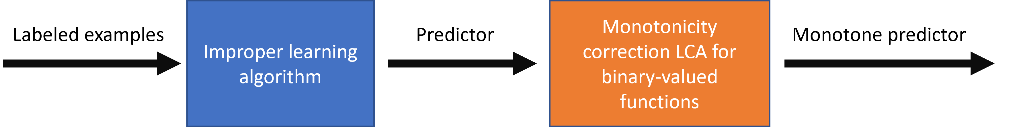
Figure 1: Control-flow diagram of the semiagnostic algorithm of [LRV22]

This way, [LRV22] obtain a succinct polytime-evaluable description of a monotone function $g_{\text{mon}}$ for which $\mathrm{dist}(f,g_{\text{mon}})\leq 3\cdot\mathrm{dist}(f,f_{\text{mon}})+\varepsilon$.

However, one can see that even if the correction constant $c$ in Equation 1 were equal to $1$ (which is the best it can be) this approach could only yield a guarantee of $\mathrm{dist}(f,g_{\text{mon}})\leq 2\cdot\mathrm{dist}(f,f_{\text{mon}})+\varepsilon$.

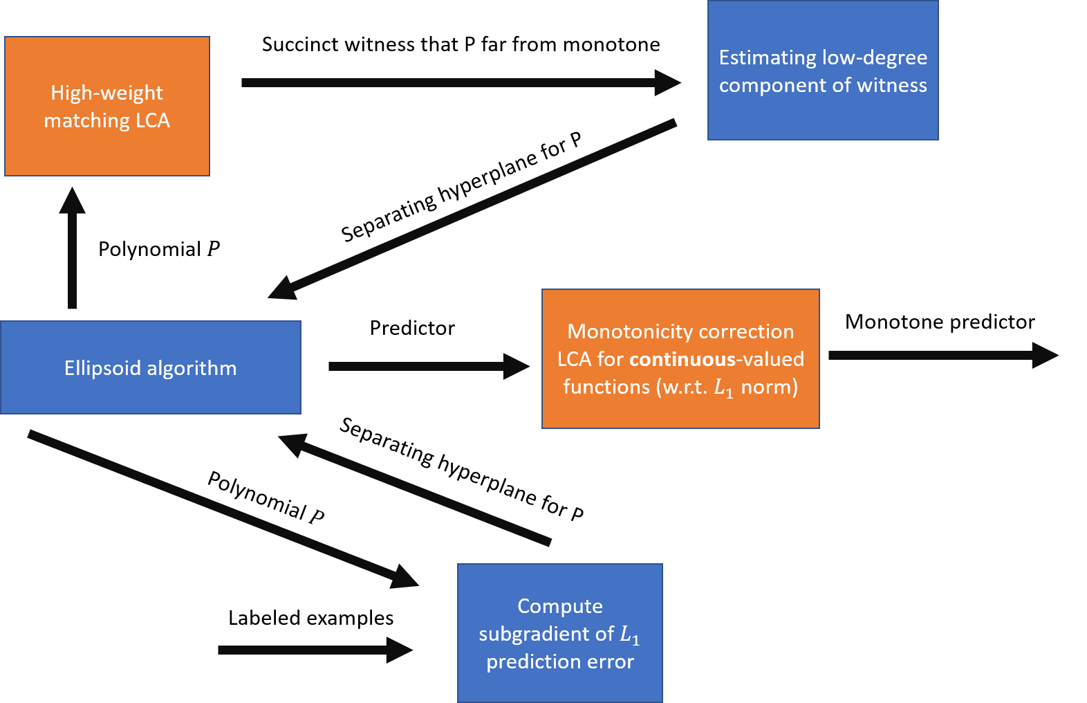
Figure 2: Control-flow diagram of the fully agnostic learning algorithm presented in this work

1.3.1 Description of our approach

We overcome this barrier by using a different approach, summarized in Figure 2. As before, there is an improper learning phase and a correction phase; however in both phases we work with real-valued functions. We have essentially three steps:

1. Find a real-valued polynomial $P$ that is $\varepsilon$-close to some monotone function, $(\alpha+\varepsilon)$-close to the unknown function $f$ in $\ell_{1}$ distance, and bounded in $[-1,1]$.

2. Obtain a succinct description of a real-valued function $P_{\text{CORRECTED}}$ that is monotone, and $O(\varepsilon)$-close to $P$ in $\ell_{1}$ distance.

3. Round the real-valued function $P_{\text{CORRECTED}}$ to be $\{\pm 1\}$-valued, while preserving monotonicity and closeness to $f$.

In contrast to the approach of [LRV22], the improper learning phase is constrained to produce a good predictor that is $\varepsilon$-close to some monotone function, regardless of how far $f$ may be from monotone. Existing improper learning algorithms are far from satisfying this new requirement. We design a new improper learner by combining the polynomial-approximation based techniques of [BT96, KKMS05, FKV20] with graph LCAs and the ellipsoid method for convex optimization.

The improper learning task is a convex feasibility problem; the set of polynomials satisfying the constraints we give in step (1) is a convex subset of the initial convex set of low-degree real polynomials. The ellipsoid method requires a separation oracle, i.e. some way to efficiently generate a hyperplane separating a given infeasible polynomial from the feasible region. Such hyperplanes are themselves low-degree real polynomials, which have high inner product with the infeasible polynomial and low inner product with every point in the feasible region. The separator for the set of polynomials that are $(\alpha+\varepsilon)$-close to $f$ is, as shown in Figure 2, just the gradient of the prediction error; the more interesting case is the separator for the set of polynomials that are $\varepsilon$-close to monotone.

With an argument inspired by the characterization of Lipschitz functions given in [BRY14], we observe that if a real-valued polynomial $P$ is far from monotone, this can be witnessed by a large matching on the pairs of elements on which $P$ violates monotonicity. Given any description of the matching, we show how to extract a separating hyperplane for $P$ by evaluating the matching on a set of sample points. Therefore, the challenge is to find a description of a sufficiently large matching that can also be evaluated quickly. We elaborate on this in the next section.

Step (2) requires another technical contribution, which is an extension of the poset-sorting LCA of [LRV22] to real-valued functions. This extension is crucial for us to achieve the overall agnostic learning guarantee, because in the improper learning phase we obtain a real-valued function that is only close to monotone in $\ell_{1}$ distance. For step (3) we use the rounding procedure of [KKMS05] that rounds real-valued functions to $\{\pm 1\}$-valued functions, and we show that this procedure also preserves monotonicity.

1.3.2 LCAs and succinct representations of large objects

In this work we employ heavily the concept of a succinct representation. The succinct representations we deal with will have size and evaluation time $2^{\tilde{O}(\sqrt{n}/\varepsilon)}$. To be fully specific, we consider succinct representations of two types of objects:

• A succinct representation of a function $f:\{\pm 1\}^{n}\rightarrow\mathbb{R}$ is an algorithm that, given $x\in\{\pm 1\}^{n}$, computes $f(x)$ in time $2^{\tilde{O}(\sqrt{n}/\varepsilon)}$.

• A succinct representation of a (possibly weighted) graph $G$ with the vertex set $\{\pm 1\}^{n}$ is an algorithm that, given $v\in\{-1,1\}^{n}$, outputs all its neighbors and the weights of corresponding edges in time $2^{\tilde{O}(\sqrt{n}/\varepsilon)}$.

A polynomial of degree $O(\sqrt{n})$ is an example of a succinct representation, but another type of representation that makes frequent appearances in this work is a local computation algorithm, or LCA [ARVX12, RTVX11]. An LCA efficiently computes a function over a large domain. For example, an LCA for an independent set takes as input some vertex $v$, makes some lookups to the adjacency list of the graph, then outputs “yes” or “no” so that the set of vertices for which the LCA would output “yes” form an independent set. Typically, its running time and query complexity are each sublinear in the domain size. We require that all LCAs used in this work have outputs consistent with one global object, regardless of the order of user queries, and without remembering any history from previous queries. This property allows us to use the LCA, in conjunction with any succinct representation of the graph, as a succinct representation of the object it computes. We formalize this relationship in Section 2.4.

1.4 Other related work

The local correction of monotonicity was studied in [ACSL08, SS10, BGJ⁺10, AJMR14] and [LRV22] (see [LRV22] for an overview of previously available algorithms for monotonicity correction and lower bounds).

The work of [CGG⁺16] gives an improper learning algorithm for a function class that is larger than monotone functions. Additionally, we note that testing of monotone functions has also been studied over hypergrids [CS13, BRY14, BCS18, BCS20].

In addition to [Gha22], there have been many exciting recent works on local computation algorithms (LCAs). Some examples include [RTVX11], [ARVX12], [LRY17], [GHL⁺15], [RV16], [EMR14], [Gha15],
[CFG⁺19], [ELMR21] , [PRVY19], [GU19],[LRR20], [AL21], [BGR21] and [GR21].

2 Preliminaries

2.1 Posets and $\{-1,1\}^{n}$

Let $P$ be a partially-ordered set. We use $\preceq$ to denote the ordering relation on $P$. We say $x\prec y$ (“$x$ is a predecessor of $y$”) if $x\preceq y$ and $x\neq y$, and use the analogous symbols $\succeq$ and $\succ$ for successorship. If $x\prec y$ and there is no $z$ in $P$ for which $x\prec z\prec y$, then $x$ is an immediate predecessor of $y$ and $y$ is an immediate successor of $x$. We refer to the poset $P$ and its Hasse diagram (DAG) interchangeably. The transitive closure $TC(P)$ is the graph on the elements of $P$ that has an edge from each vertex to each of its successors. A succinct representation of $P$ with size $s$ is any function stored in $s$ bits of memory that takes as input the identity of a vertex, outputs the sets of immediate predecessors and immediate successors, and runs in time $O(s)$ in the worst case over vertices.

Specific posets of interest in this work are the Boolean cube and the weight-truncated cube. We give a definition and a size-$O(n/\varepsilon)$ representation computing the truncated cube.

Definition 1.

The $n$-dimensional Boolean hypercube is the set $\{-1,1\}^{n}$. For $x,y\in\{-1,1\}^{n}$, we say $x\preceq y$ if for all $i\in\{1,\cdots,n\}$ one has $x_{i}\leq y_{i}$. It is immediate that $\{-1,1\}^{n}$ is a poset with $2^{n}$ elements.

We also define the truncated hypercube

$$H^{n}_{\varepsilon}:=\left\{x\in\{-1,1\}^{n}:~{}\left|\sum_{i}x_{i}\right|\leq\sqrt{2n\log\frac{2}{\varepsilon}}\right\},$$

Via Hoeffding’s bound, we have that the fraction of elements in $\{0,1\}^{n}$ that are not also in $H_{n}^{\varepsilon}$ is at most $2\exp\left(-\frac{2t^{2}}{4n}\right)=\varepsilon$.

For $i\in[n]$, let $e_{i}$ be the vector that is $1$ at index $i$ and $-1$ everywhere else.

Given: Input $x\in\{-1,1\}^{n}$, truncation parameter $\varepsilon$

return $\{x\oplus e_{i}~{}|~{}i\in[n]\text{ and }|\sum_{j}(x\oplus e_{i})_{j}|\leq\sqrt{2n\log\frac{2}{\varepsilon}}\}$

Algorithm 1 LCA: TruncatedCube$(x,\varepsilon)$

2.1.1 Fourier analysis over $\{\pm 1\}^{n}$.

Let $[n]$ denote the set $\{1,2,\cdots,n\}$. We define for every $S\subseteq[n]$ the function $\chi_{S}:\{\pm 1\}^{n}\rightarrow\mathbb{R}$ as $\chi_{S}(\bm{x}):=\prod_{i\in S}x_{i}.$ We define the inner product between two functions $g_{1},g_{2}:\{\pm 1\}^{n}\rightarrow\mathbb{R}$ as follows: $\langle g_{1},g_{2}\rangle:=\mathbb{E}_{\bm{x}\sim\{\pm 1\}^{n}}\left[g_{1}(\bm{x})g_{2}(\bm{x})\right]$. It is known that $\langle\chi_{S_{1}},\chi_{S_{2}}\rangle=\mathbbm{1}_{S_{1}=S_{2}}$. For a function $g:\{\pm 1\}^{n}\rightarrow\mathbb{R}$ we denote $\widehat{g}(S):=\langle g,\chi_{S}\rangle$. It is known that

$$g(\bm{x}) =\sum_{S\subseteq[n]}\widehat{g}(S)\chi_{S}(\bm{x}) \langle g_{1},g_{2}\rangle =\sum_{S\subseteq[n]}\widehat{g}_{1}(S)\widehat{g}_{2}(S).$$

2.2 Monotone functions

Part of our algorithm concerns monotonicity of functions over general posets. For a function $f:P\to\mathbb{R}$, we say that a pair of elements $x,y\in P$ forms a violated pair if we have $x\preceq y$ but $f(x)>f(y)$, and we define the violation score $\mathrm{vs}(x,y):=f(x)-f(y)$. The violation graph $\mathrm{viol}(f)$ is the subgraph of $TC(P)$ induced by violated pairs in $f$. The weight of an edge is the difference $f(x)-f(y)$.

The $\ell_{1}$ distance of $f$ to monotonicity $\mathrm{dist}(f,\mathrm{mono})$ is the $\ell_{1}$ distance of $f$ to the closest real-valued monotone function.

Definition 2 (Distance to monotonicity).

The $\ell_{1}$ distance of $f:P\to\mathbb{R}$ to monotonicity is its distance to the closest real-valued monotone function.

$$\mathrm{dist}_{1}(f,\mathrm{mono}):=\min_{\text{monotone }g:P\to\mathbb{R}}\bigg{[}\frac{1}{|P|}\sum_{x\in P}|f(x)-g(x)|\bigg{]}$$

The Hamming distance to monotonicity of $f:P\to\{-1,1\}$ is defined analogously.

$$\mathrm{dist}_{0}(f,\mathrm{mono}):=\min_{\text{monotone }g:P\to\{-1,1\}}\bigg{[}\frac{1}{|P|}\sum_{x\in P}\mathds{1}[f(x)\neq g(x)]\bigg{]}$$

We will need a bound on how well monotone functions can be approximated by low-degree polynomials. The following fact follows from [BT96, KKMS05] and a refinement by [FKV20].

Fact 2.1.

For every monotone $f:\{-1,1\}^{n}\to\{-1,1\}$ and $\varepsilon>0$, there exists a multilinear polynomial $p$ of degree $\lceil\frac{4\cdot\sqrt{n}}{\varepsilon}\log\frac{4}{\varepsilon}\rceil$ such that

$$||f-p||_{1}\leq\varepsilon.$$

2.3 Convex optimization

Definition 3.

A separation oracle for a convex set $\mathcal{C}_{\text{convex}}$ is an oracle that given a point $\bm{x}$ does one of the following things:

• If $x\in\mathcal{C}_{\text{convex}}$, then the oracle outputs “Yes”.

• If $x\notin\mathcal{C}_{\text{convex}}$, then the oracle outputs $(\text{No},q_{\text{separation}})$, where $Q_{\text{separation}}\in\mathbb{R}^{d}$ represents a direction along which $x$ is separated from $\mathcal{C}_{\text{convex}}$. Formally, $\langle Q_{\text{separation}},x\rangle>\langle Q_{\text{separation}},x^{\prime}\rangle$ for any $x^{\prime}$ in $\mathcal{C}_{\text{convex}}$.

Fact 2.2.

There is an algorithm EllipsoidAlgorithm that takes as inputs positive real values $r$ and $R$, and access to a separation oracle for some convex set $\mathcal{C}_{\text{convex}}\subset\{x\in\mathbb{R}^{d}:\quad\left\|x\right\|\leq R\}$. The algorithm runs in time $\mathop{poly}\left(d,\log\frac{R}{r}\right)$ and either outputs an element in $\mathcal{C}_{\text{convex}}$ or outputs FAIL. Furthermore, if $\mathcal{C}_{\text{convex}}$ contains a ball of radius $r$, the algorithm is guaranteed to succeed.

2.4 LCAs and succinct representations

We use the following LCAs in this work:

Theorem 3 (LCA for maximal matching [Gha22]).

There is an algorithm GhaffariMatching that takes all-neighbor access to a graph $G$, with $N$ vertices and largest degree at most $\Delta$, a random string $r\in\{0,1\}^{\mathop{poly}(\Delta,\log(N/\delta))}$, parameter $\delta\in(0,1)$ and a vertex $v\in G$. The algorithm outputs the identity of a vertex $u:(u,v)\in E(G)$ or $\bot$. The algorithm runs in time $\mathop{poly}(\Delta,\log(N/\delta))$ and with probability at least $1-\delta$ over the choice of $r$ the condition of global consistency holds i.e. the set of edges $\{(u,v)\in G:\,\text{GhaffariMatching}(G,r,\delta,u)=v\}$ is a maximal matching in the graph $G$.

Theorem 4 (LCA for monotonicity correction of Boolean-valued functions [LRV22]).

There is an algorithm BooleanCorrector that takes access to a function $f:P\to\{-1,1\}$ and all-neighbor access to a poset $P$ with $N$ vertices, such that each element has at most $\Delta$ predecessors and successors and the longest directed path has length $h$, a random string $r\in\{0,1\}^{\mathop{poly}(\Delta,\log(N/\delta))}$, a parameter $\delta\in(0,1)$ and an element $x$ in $P$. The algorithm outputs a value in $\{-1,1\}$. The algorithm runs in time $\Delta^{O(\log h)}\cdot\mathop{polylog}(N/\delta)$ and with probability at least $1-\delta$ over the choice of $r$ the condition of global consistency holds i.e. the function $g:P\to\{-1,1\}$ defined as $g(x):=\text{BooleanCorrector}(P,r,\delta,x)$ is monotone and is such that $\operatorname{{Pr}}_{x\sim P}[g(x)\neq f(x)]\leq 2\cdot\mathrm{dist}(f,\mathrm{mono})$.

An important idea in [LRV22] is that LCAs (i.e. algorithms that achieve global consistency) can be used to operate on succinct representations of combinatorial objects. To explain further, we need the following definition:

Definition 4 (Succinct representation).

A succinct representation of a function $f$ of size $s$ is a a description of $f$ that is stored in $s$ bits of memory and can be evaluated on an input in $O(s)$ time.

For example, circuits of size $s$ and polynomials of degree $\log s$ are examples of succinct representations of size $s$. The following fact follows immediately from the definition:

Fact 2.3 (Composition of representations).

If a function $f$ has a description that uses $t$ bits of memory and evaluates in time $O(t)$ given oracle queries to a function $g$, and $g$ has a succinct representation of size $s$, then there is a succinct representation of $f$ of size $O(t+sq)$.

Now, for example, combining 2.3 and Theorem 3 we see immediately that for a graph $G$, with $N$ vertices and largest degree at most $\Delta$, using the algorithm in Theorem 3 we can transform a size-$s$ representation of a function computing all-neighbor access to $G$ into a size-$\left(\Delta^{O(\log h)}\cdot\mathop{polylog}(N/\delta)\cdot s\right)$ representation of a function that determines membership in some maximal matching over $G$. Note that this transformation itself runs in time $\Delta^{O(\log h)}\cdot\mathop{polylog}(N/\delta)\cdot s$. Analogously, in an exact same fashion it is possible to combine 2.3 and Theorem 4.

3 Our algorithms

In this section we give descriptions of the agnostic learning algorithm and its major components (we will analyze the algorithms in the subsequent sections). The algorithm MonotoneLearner makes calls to
EllipsoidAlgorithm, where the optimization domain is the $\leq n^{\left\lceil\frac{4\cdot\sqrt{n}}{\varepsilon}\log\frac{4}{\varepsilon}\right\rceil}$-dimensional space of degree-$\left\lceil\frac{4\cdot\sqrt{n}}{\varepsilon}\log\frac{4}{\varepsilon}\right\rceil$ polynomials over $\mathbb{R}^{n}$, and its output, $P^{\text{GOOD}}$, is such a polynomial (see 2.2 for details). It also makes calls to HypercubeCorrector, which is given in Corollary 4.7.

1:Given: Integer $n$, $\varepsilon\in(0,1)$, and uniform sample access to an unknown function $f:\{\pm 1\}^{n}\rightarrow\{\pm 1\}$.

2:Output: Circuit $\mathcal{C}:\{\pm 1\}^{n}\rightarrow\{\pm 1\}$.

3:for $\alpha\in\{\varepsilon,2\varepsilon,3\varepsilon,\cdots 1-\varepsilon,1+200\varepsilon\}$ do

4:     $\text{OptimizationResult}\leftarrow\textsc{EllipsoidAlgorithm}\left(1,\varepsilon\cdot n^{-\frac{1}{2}\left\lceil\frac{4\cdot\sqrt{n}}{\varepsilon}\log\frac{4}{\varepsilon}\right\rceil},\textsc{Oracle}_{\alpha,n,\varepsilon}\right)$.

5:     if OptimizationResult$\neq$FAIL then

6:         $P^{\text{GOOD}}=\text{OptimizationResult}$

7:         $P^{\text{GOOD}}_{\text{TRIMMED}}\leftarrow$ representation of a function that takes input $\bm{x}$ and outputs the value $\begin{cases}P^{\text{GOOD}}(x)&\text{if }P^{\text{GOOD}}(x)\in[-1,+1]\\ 1&\text{if }P^{\text{GOOD}}(x)>1\\ -1&\text{if }P^{\text{GOOD}}(x)<-1\end{cases}$

8:         $P^{\text{GOOD}}_{\text{CORRECTED}}\leftarrow$ representation of a function that takes input $\bm{x}$ and returns the value $\textsc{HypercubeCorrector}(x,P^{\text{GOOD}}_{\text{TRIMMED}},r)$

9:         $T\leftarrow\frac{200}{\varepsilon^{2}}\log\left(\frac{20}{\varepsilon}\right)\log(20n)$ i.i.d. pairs $(\bm{x}_{i},f(\bm{x}_{i}))$, with $\bm{x}_{i}$ sampled uniformly from $\{-1,1\}^{n}$.

10:         ThresholdCandidates$\leftarrow\left\{\frac{1}{\varepsilon}\text{ i.i.d. uniformly random elements in }[-1,1]\right\}$.

11:         $t^{*}:=\operatorname*{arg\,min}_{t\in\text{ThresholdCandidates}}\left[\frac{1}{|T|}\sum_{\bm{x}\in T}\left[\left|\mathbb{\text{sign}}(P_{\text{GOOD, TRIMMED, CORRECTED}}(\bm{x})-t)-f(\bm{x})\right|\right]\right]$

12:         return representation of a function that takes input $\bm{x}$ and returns the value $\mathbb{\text{sign}}(P_{\text{GOOD, TRIMMED, CORRECTED}}(\bm{x})-t)^{*}$

13:     end if

14:end for

Algorithm 2 Algorithm MonotoneLearner $(n,\varepsilon,T)$

The subroutine Oracle takes as input a polynomial and provides the separating hyperplane required by EllipsoidAlgorithm. It makes calls to HypercubeMatching (see Lemma 5.4), which provides a high-weight matching over the pairs of labels that violate monotonicity.

1:Given: $\varepsilon,\alpha\in(0,1)$, degree-$\left\lceil\frac{4\cdot\sqrt{n}}{\varepsilon}\log\frac{4}{\varepsilon}\right\rceil$ polynomial $P$ over $\mathbb{R}^{n}$ with $\left\|P\right\|_{2}\leq 1$, and uniform sample access to an unknown function $f:\{\pm 1\}^{n}\rightarrow\{\pm 1\}$.

2:Output: ”Yes” or (”No”, $Q_{\text{separator}}$), where $Q_{\text{separator}}$ is a degree-$\left\lceil\frac{4\cdot\sqrt{n}}{\varepsilon}\log\frac{4}{\varepsilon}\right\rceil$ polynomial over $\mathbb{R}^{n}$.

3:$P_{\text{TRIMMED}}\leftarrow$ representation of a function that takes input $\bm{x}$ and outputs $\begin{cases}P(x)&\text{if }P(x)\in[-1,+1]\\ 1&\text{if }P(x)>1\\ -1&\text{if }P(x)<-1\end{cases}$.

4: $T\leftarrow$ set of $n^{\frac{C\sqrt{n}}{\varepsilon}\log\frac{1}{\varepsilon}}$ i.i.d. pairs $(\bm{x}_{i},f(\bm{x}_{i}))$, with $\bm{x}_{i}$ sampled uniformly from $\{-1,1\}^{n}$ (for sufficiently large constant $C$).

5:$r\leftarrow$ string of $2^{C\sqrt{n}(\log n\cdot\log\frac{1}{\varepsilon})^{C}}$ random i.i.d. bits (for sufficiently large constant $C$).

6: $M_{\text{separator}}\leftarrow$ representation of a function that takes input $x$ and outputs $\begin{cases}0&\text{if }\textsc{HypercubeMatching}(P_{\text{TRIMMED}},\varepsilon/4,r)\text{ does not match $x$ to any other vertex}\\ 1&\text{if }\textsc{HypercubeMatching}(P_{\text{TRIMMED}},\varepsilon/4,r)\text{ matches $x$ some vertex $z$, s.t. $z\preceq x$}\\ -1&\text{if }\textsc{HypercubeMatching}(P_{\text{TRIMMED}},\varepsilon/4,r)\text{ matches $x$ some vertex $z$, s.t. $z\succeq x$}\end{cases}$

7:if $\frac{1}{|T|}\sum_{\bm{x}\in T}\left[M_{\text{separator}}(\bm{x})\cdot P_{\text{TRIMMED}}(\bm{x})\right]>5\varepsilon$ then

8:     $Q_{\text{separator}}\leftarrow\sum_{S\subset[n]:\>\left|S\right|\leq\left\lceil\frac{4\cdot\sqrt{n}}{\varepsilon}\log\frac{4}{\varepsilon}\right\rceil}\left(\frac{1}{|T|}\sum_{\bm{x}\in T}\left[M_{\text{separator}}(\bm{x})\cdot\chi_{S}(\bm{x})\right]\right)\chi_{S}$

9:     return (”No”, $Q_{\text{separator}}$)

10:else if $\frac{1}{|T|}\sum_{\bm{x}\in T}\left[\left|f(\bm{x})-P(\bm{x})\right|\right]>\alpha+50\varepsilon$ then

11:     $Q_{\text{separator}}\leftarrow\sum_{\begin{subarray}{c}S\subset[n]\left|S\right|\leq\left\lceil\frac{4\cdot\sqrt{n}}{\varepsilon}\log\frac{4}{\varepsilon}\right\rceil\end{subarray}}\left(\mathbb{E}_{\bm{x}\sim T}\left[\widehat{P}(S)\chi_{S}(\bm{x})\mathbb{\text{sign}}(P(\bm{x})-f(\bm{x}))\right]\right)\chi_{S}$

12:     return (”No”, $Q_{\text{separator}}$)

13:else

14:     return ”Yes”

15:end if

Algorithm 3 Subroutine $\textsc{Oracle}_{\alpha,n,\varepsilon}(P)$

The algorithm MatchViolations finds a high-weight matching on the violation graph of a poset. It is the main component of HypercubeMatching, which is just a wrapper that calls MatchViolations on the truncated cube. FilterEdges removes vertices that are either incident to $M$ or have weight below the threshold $t$, and GhaffariMatching is the maximal matching algorithm of Theorem 3. More implementation details and analysis are given in Section 5.

Given: Poset $P$ and function $f:~{}P\to[-1,1]$ given as succinct representations, weight threshold $\varepsilon$, random seed $r$

Output: Succinct representation of a high-weight matching on the violating pairs of $P$ w.r.t. $f$

if $\varepsilon<1/|P|$ then

     $M\leftarrow$ representation of the greedy algorithm that adds each edge $(x,y)$ of $TC(P)$ in decreasing order of $f(x)-f(y)$.

else

     $t\leftarrow 2$

     $M\leftarrow$ representation of a function computing the empty matching

     while $t>\varepsilon/2$ do

         $P^{\prime}\leftarrow$ representation of a function that takes input $x$ and outputs

FilterEdges$(TC(P),f,t,M,x)$

         $M\leftarrow$ representation of a function that takes input $x$ and outputs $M(x)$ if $M(x)\neq\bot$, otherwise GhaffariMatching$(P^{\prime},r,x))$

         $t\leftarrow t/2$

     end while

end if

return $M$

Algorithm 4 MatchViolations$(P,f,\varepsilon,r)$

The following is the core of HypercubeCorrector, given as a “global overview” for convenience. Analysis and local implementation are given in Section 4. The algorithm corrects monotonicity of a $k$-valued function over a poset. HypercubeCorrector is a wrapper that discretizes a real-valued function and then calls this corrector with the truncated hypercube as the poset.

1:Given: Poset $P$ of height $h$, function $f:P\to[k]$

2:Output: monotone function $g:P\to[k]$

3:Let $i\leftarrow 0$

4:for $0\leq i\leq\lceil\log k\rceil$ do

5:     Let $f_{i}$ be the projection of $f$ onto the $i_{th}$ most significant bit of $k$, i.e. $f_{i}(x)=1$ if the $i_{th}$ bit of $f(x)$ is $1$.

6:     Let $P_{i}$ be the poset on the elements of $P$ with the relation

$$x\prec_{P_{i}}y:=x\prec_{P}y\text{ and }f_{j}(x)=f_{j}(y)\text{ for all $j<i$}.$$

7:     Let $\pi_{i}\leftarrow$ BooleanCorrector$(f_{i},P_{i})$.

8:     Let $f\leftarrow f\pi_{i}$.

9:end for

10:return $f$

Algorithm 5 Global view of sorting $k$-valued labels in a poset

4 Analysis of the local corrector

In this section, we prove Theorem 2 by analyzing our algorithm for correcting a real-valued function over a poset in a way that preserves the $\ell_{1}$ distance to monotonicity within a factor of 2. This extends the monotonicity corrector of [LRV22] to handle functions with non-Boolean ranges.

Lemma 4.1 ($\ell_{1}$ correction of $k$-valued functions).

Let $P$ be a poset and $f:P\to[k]$ be $\alpha$-close to monotone in $\ell_{1}$ distance. There is an LCA that makes queries to $f$ and outputs queries to $g:P\to[k]$, such that $g$ is monotone and $||f-g||_{1}\leq 2\alpha$. The LCA makes $(\Delta\log N)^{O(\log h\log k)}$ queries, where $\Delta$ is the maximum number of predecessors or successors of any element in $P$, $N$ is the number of vertices, and $h$ is the length of the longest directed path.. It uses a random seed of length $\mathop{poly}(\Delta\log N)$, and succeeds with probability $1-N^{-10}$.

The following lemmas are used in the proof of correctness of our algorithm. Their proofs are deferred to the appendix.

Lemma 4.2 (Equivalence of $k$-valued and bitwise monotonicity).

Let $f:P\to[k]$ be a function and $f_{i}$ be the projection of $f$ onto the $i_{th}$ most significant bit of $k$, i.e. $f_{i}(x)=1$ if the $i_{th}$ bit of $f(x)$ is $1$, for each $i\in[\lceil\log k\rceil]$. Let $P_{i}$ be the poset on the elements of $P$ with the relation

$$x\prec_{P_{i}}y:=x\prec_{P}y\text{ and }f_{j}(x)=f_{j}(y)\text{ for all $j<i$}.$$

Then $f$ is monotone if and only if each $f_{i}$ is monotone over the corresponding $P_{i}$.

Lemma 4.3 (Preservation of closeness to monotone functions).

Let $g$ be obtained from $f$ by swapping the labels of a pair $x\prec_{P}y$ that violates monotonicity. Then for any monotone function $m$, $||g-m||_{1}\leq||f-m||_{1}$.

The corollary follows from repeated application of Lemma 4.3 and the triangle inequality.

Corollary 4.4 ($\ell_{1}$ error preservation).

Let $g$ be obtained from $f$ by a series of swaps of label pairs that violate monotonicity in $f$. Then $||g-f||_{1}\leq 2\cdot\mathrm{dist}_{1}(f,\mathrm{mono})$.

We also require a modification to the LCA claimed in Theorem 4 for correcting Boolean functions. That algorithm works by performing a sequence of label-swaps on pairs that violate monotonicity in the poset, then outputting the function value that ends up at the queried vertex $x$. It can instead track the swaps and output the identity of the vertex that $x$ receives its final label from. The modified algorithm can be thought of as an LCA that gives query access to a label permutation.

Fact 4.5 (Poset sorting algorithm implicit in [LRV22]).

Let $P$ be a poset with $N$ vertices such that every element has at most $\Delta$ predecessors and successors, and the longest directed path has length $h$. Let $f:P\to\{-1,1\}$ be $\alpha$-close to monotone in Hamming distance. There is an algorithm BooleanCorrector that gives query access to a permutation $\pi$ of $P$ such that $f\pi$ is a monotone function and $\operatorname{{Pr}}_{x\sim P}[f(x)\neq(f\pi)(x)]\leq 2\alpha$. The LCA implementation of BooleanCorrector uses $(\Delta\log N)^{O(\log h)}$ queries and running time, has a random seed of length $\mathop{poly}(\Delta\log N)$, and succeeds with probability $1-N^{-11}$.

Here we present the LCA implementation of Algorithm 5.

1:Given: Target vertex $x$, all-neighbors (immediate predecessor and successor) oracle for $P$, query access to $f:P\to[k]$, iteration number $i$, random seed $r$.

2:Output: query access to function $g:P\to[k]$ which is monotone when truncated to the first $i$ most significant bits.

3:if $i=0$ then return $f(x)$

4:else

5:     $S\leftarrow$ the set of all predecessors and successors of $x$ in $P$

6:     for $y\in S$ do

7:         Let $f^{\prime}(y)\leftarrow$$k$-Corrector$(y,P,f,i-1,r)$.

8:     end for

9:     Let $f^{\prime}_{i}$ be defined as in Algorithm 5, and $P^{\prime}_{i}$ be similarly defined with respect to $f^{\prime}_{i}$.

10:     Remove any $y$ from $S$ such that $f^{\prime}_{i}(y)=f^{\prime}_{i}(x)$ or $y$ and $x$ are incomparable in $P^{\prime}_{i}$.

11:     Let $z\leftarrow$ BooleanCorrector$(x,P^{\prime}_{i},f^{\prime}_{i},r)$

12:     return $f^{\prime}(z)$

13:end if

Algorithm 6 LCA implementation of Algorithm 5, $k$-Corrector$(x,P,f,i,r)$

Given: function $f:\{-1,1\}\to[-1,1]$ given as succinct representation, additive error parameter $\varepsilon>0$, random seed $r$.

Output: succinct representation of monotone function $g:\{-1,1\}\to[-1,1]$.

$P\leftarrow$ representation of a function that takes $x$ and outputs TruncatedCube$(x,\varepsilon)$

$f^{\prime}\leftarrow$ representation of a function that takes $x$ and outputs $\lfloor f(x)/\varepsilon\rfloor$

$f^{\prime\prime}\leftarrow$ representation of a function that takes $x$ and outputs

$\indent\begin{cases}\varepsilon\cdot k\text{\sc-Corrector}(x,P,f^{\prime},\lceil\log(1/\varepsilon)\rceil,r)&-\sqrt{2n\log 2/\varepsilon}\leq|x|\leq\sqrt{2n\log 2/\varepsilon}\\ 1&|x|\geq\sqrt{2n\log 2/\varepsilon}\\ -1&|x|\leq-\sqrt{2n\log 2/\varepsilon}\end{cases}$

return $f^{\prime\prime}$

Algorithm 7 HypercubeCorrector$(f,\varepsilon,r)$

Lemma 4.6 (Correctness and query complexity of Algorithm 6).

With probability $1-i\cdot N^{-11}$ over a random seed $r$ of length $\mathop{poly}(\Delta\log N)$, the algorithm $k$-Corrector$(x,P,f,i,r)$ gives query access to a function $g$ that is monotone when truncated to the first $i$ most significant bits. Its query complexity is $(\Delta\log N)^{O(i\log h+1)}$, and $||g-f||_{1}\leq 2\alpha$, where $\alpha$ is the $\ell_{1}$ distance of $f$ to the nearest monotone function.

Proof.

Fix the random seed $r$ and assume all calls to BooleanCorrector succeed with $r$, then we proceed by induction. In the base case, $f$ is certainly monotone when truncated to 0 bits and the algorithm makes only 1 query. In the inductive case, suppose the claim holds for $i-1$; in other words $k$-Corrector$(y,P,f,i-1,r)$ makes $(\Delta\log N)^{O((i-1)\log h+1)}$ queries and returns a function that is monotone in the first $i-1$ bits. Then when $k$-Corrector is called with iteration number $i$, the function $f^{\prime}_{j}$ is monotone over $P^{\prime}_{j}$ for all $j<i$. BooleanCorrector$(x,P^{\prime}_{i},f^{\prime}_{i},r)$ returns a vertex to swap labels with $x$ such that the resulting function is monotone in the $i_{th}$ bit, over the poset $P^{\prime}_{i}$. Then the function returned by $k$-Corrector satisfies the conditions of Lemma 4.2 for the first $i$ bits, so it must be monotone in the first $i$ bits.

We now bound the failure probability and distance to $f$. The failure probability of BooleanCorrector is $N^{-11}$ and we call BooleanCorrector on $i$ different graphs, so by union bound the total failure probability is $\leq i\cdot N^{-11}$ as desired. The fact that $||g-f||_{1}\leq 2\alpha$ follows from Corollary 4.4. ∎

We can now prove Theorem 2.

See 2

Proof of Theorem 2.

Given some $\varepsilon\in(0,1/2)$, let $f_{\varepsilon}(x):=\lfloor f(x)/\varepsilon\rfloor$; certainly queries to $f_{\varepsilon}$ can be simulated by queries to $f$. On input $x$, run $k$-Corrector$(x,P,f_{\varepsilon},\lceil\log(2/\varepsilon)\rceil,r)$ with a random seed $r$ of length $\mathop{poly}(\Delta\log N)$. By Lemma 4.6, this makes $(\Delta\log N)^{O(\log(1/\varepsilon)\log h)}$ queries to $f_{\varepsilon}$ and outputs $g_{\varepsilon}(x)$, where $g$ is monotone and $||g_{\varepsilon}-f_{\varepsilon}||_{1}\leq 2\cdot\mathrm{dist}_{1}(f_{\varepsilon},\mathrm{mono})$. Since $f$ is $\alpha$-close to some monotone function $m$, we have $\mathrm{dist}_{1}(f_{\varepsilon},\mathrm{mono})\leq||f_{\varepsilon}-m/\varepsilon||_{1}\leq||f/\varepsilon-m/\varepsilon||_{1}+||f/\varepsilon-f_{\varepsilon}||_{1}\leq\alpha/\varepsilon+1$.

Return $g(x):=\varepsilon\cdot g_{\varepsilon}(x)$. Then

$$||g-f||_{1}=||\varepsilon g_{\varepsilon}-f||_{1}\leq||\varepsilon g_{\varepsilon}-\varepsilon f_{\varepsilon}||_{1}+||\varepsilon f_{\varepsilon}-f||_{1}\leq 2\varepsilon(\alpha/\varepsilon+1)+\varepsilon\leq 2\alpha+3\varepsilon.$$

The failure probability is $N^{-11}\cdot\lceil\log(2/\varepsilon)\rceil$ by Lemma 4.6, but we will assume that $\lceil\log(2/\varepsilon)\rceil<N$. Otherwise, the allowed query complexity and running time would exceed $\Delta^{N}$, which is $>\Delta N$ for any $\Delta,N>1$. With $O(\Delta N)$ query complexity and running time, a trivial algorithm would suffice: one could solve the linear program with $\Delta N$ monotonicity constraints, minimizing $||g-f||_{1}$. Under our assumption, the failure probability is at most $N^{-10}$. ∎

Corollary 4.7 (Monotonizing a representation of a function on the Boolean cube).

Let $f:\{-1,1\}^{n}\to[-1,1]$ be $\alpha$-close to monotone in $\ell_{1}$ distance, given as a succinct representation of size $s_{f}$. There is an algorithm that runs in time $2^{\tilde{O}(\sqrt{n}\log^{3/2}(1/\varepsilon))}\cdot s_{f}$ time and outputs a monotone function $g$ such that $||f-g||_{1}\leq 2\alpha+4\varepsilon$. The size of the representation of $g$ is $2^{\tilde{O}(\sqrt{n}\log^{3/2}(1/\varepsilon))}\cdot s_{f}$. The algorithm uses a random seed of length $2^{\tilde{O}(\sqrt{n}\log(1/\varepsilon))}$ and succeeds with probability $1-2^{-10n}$.

The proof of Corollary 4.7 is deferred to Appendix C.

5 Analysis of the matching algorithm

In this section we give an algorithm for generating a succinct representation of a matching over the violated pairs of the hypercube whose weight is a constant factor of the distance to monotonicity. The core of the algorithm is an LCA for finding such a matching over the violated pairs of an arbitrary poset.

Lemma 5.1 (Equivalence of distance to monotonicity and maximum-weight matching).

Let $W$ be the total weight of the maximum-weight matching of the violation graph of $f$. Then $\mathrm{dist}_{1}(f,\mathrm{mono})=W/N$.

Proof.

This proof is analogous to the proof of Lemma 3.1 of [BRY14]; see Appendix D. ∎

5.1 Details and correctness of MatchViolations

The algorithm Matchviolations given in Section 3 makes calls to an algorithm called FilterEdges, which removes vertices that have already been matched or are not incident to any heavy edges. We give the pseudocode for FilterEdges here.

1:Given: Poset $P$, function $f:~{}P\to[-1,1]$, and matching $M$ given as succinct representations, weight threshold $t$, vertex $x$

2:Output: All neighbors of $x$ in the graph of violation score $\geq t$ and not in $M$

3:return

$$\{y\in P(x)~{}|~{}\\ M(y)=\bot\text{ and }\left[(x<y\text{ and }f(x)\geq f(y)+t)\text{ or }(x>y\text{ and }f(x)\leq f(y)-t)\right]\}$$

Algorithm 8 LCA: FilterEdges$(P,f,t,M,x)$

Lemma 5.2.

Let $P$ be a poset with $N$ vertices, and let $\Delta$ be an upper bound on the number of predecessors and successors of any vertex in $P$. Then the output of the LCA MatchViolations$(P,f,\varepsilon,r)$ with a random seed $r$ of length $\mathop{poly}(\Delta,\log N)$, is a matching of weight at least $N(\textstyle\frac{1}{4}\mathrm{dist}_{1}(f,\mathrm{mono})-\varepsilon)$ with probability at least $1-N^{-10}$.

Proof.

This is a small modification to the standard greedy algorithm for high-weight matching; see Appendix D. ∎

Lemma 5.3 (Running time and output size).

Let $P,f,\varepsilon,N,\Delta$, and $r$ be as described in the lemma above. Let $s_{P}$ be the size of the succinct representation of $P$, and $s_{f}$ be the size of the succinct representation of $f$.

Then MatchViolations$(P,f,\varepsilon,r)$ runs in time $(\Delta\log N)^{O(\log(1/\varepsilon))}(s_{P}+s_{f})$ and outputs a representation of size $(\Delta\log N)^{O(\log(1/\varepsilon))}(s_{P}+s_{f})$.

Proof.

If $\varepsilon<1/N$, then MatchViolations constructs and outputs a representation of the standard global greedy algorithm for 2-approximate maximum matching. The representation size of this algorithm is $O(\Delta N)\leq(\Delta\log N)^{O(\log(1/\varepsilon))}$, and the running time of MatchViolations is polynomial in this representation size.

If $\varepsilon\geq 1/N$, then by induction on the number of iterations $i$, we will show that the representation size of $M$ at the start of iteration $i$ is at most $(\Delta\log N)^{O(i)}(s_{P}+s_{f})$. In the base case, we have an empty matching $M$ which has constant representation size.

In the inductive case, suppose the claim holds at the start of iteration $i$. Then we set $P^{\prime}$ to be the function that applies FilterEdges to $TC(P)$. $TC(P)$ has size $O(\Delta\cdot s_{P})$, as it makes $O(\Delta)$ calls to $P$. FilterEdges makes one call to $TC(P)$ and at most $O(\Delta)$ calls to $M$ and $f$. It also has overhead of size $O(\log t)=O(\log(1/\varepsilon))=O(\log N)$. By the inductive hypothesis, the size of $P^{\prime}$ is then

$$O(\Delta)\cdot(\Delta\log N)^{O(i)}(s_{P}+s_{f})+O(\log N)+O(\Delta\cdot s_{P})$$

$$\leq (\Delta\log N)^{O(i+1)}(s_{P}+s_{f}).$$

Then we set $M$ to be the function that applies GhaffariMatching to $P^{\prime}$. GhaffariMatching has constant overhead and makes $\mathop{poly}(\Delta,\log N)$ queries to $P^{\prime}$. Then the new size of $M$ is $\mathop{poly}(\Delta,\log N)\cdot(\Delta\log N)^{O(i)}(s_{P}+s_{f})=(\Delta\log N)^{O(i+1)}(s_{P}+s_{f})$.

The size bounds follow from the fact that there are $O(\log 1/\varepsilon)$ iterations. The corresponding running time bound for MatchViolations comes from the fact that since it only constructs the succinct representations, its running time in each iteration is polynomial in the size of the representations it constructs.

∎

1:Given: Function $f:~{}\{-1,1\}^{n}\to[-1,1]$ given as succinct representation, weight threshold $\varepsilon$, random seed $r$

2:Output: Succinct representation of a high-weight matching on the violating pairs w.r.t. $f$

3:$P\leftarrow\textsc{TruncatedCube}(n,\varepsilon)$

4:$M\leftarrow$ representation of a function that takes $x$ and outputs

5:$\begin{cases}\textsc{MatchViolations}(P,f,\varepsilon,r)&-\sqrt{2n\log 2/\varepsilon}\leq|x|\leq\sqrt{2n\log 2/\varepsilon}\\ \bot&\text{otherwise}\end{cases}$

6:return $M$

Algorithm 9 HypercubeMatching$(f,\varepsilon,r)$

Lemma 5.4.

With a random seed of length $2^{\tilde{O}(\sqrt{n}\log(1/\varepsilon))}$, Algorithm 9 outputs a representation of a matching on the weighted violation graph $\mathrm{viol}(f)$, of weight at least $2^{n}\cdot(\frac{1}{4}\mathrm{dist}_{1}(f,\mathrm{mono})-4\varepsilon)$, with probability at least $1-2^{-10n}$. The size of the representation is $2^{\tilde{O}(\sqrt{n}\log(1/\varepsilon))}\cdot s_{f}$, where $s_{f}$ is the size of the representation of $f$.

Proof.

HypercubeMatching calls MatchViolations on the truncated hypercube, which has parameters $N<2^{n}$ and $\Delta=2^{O(\sqrt{n}\log n\log(1/\varepsilon))}$. The size of the representation of TruncatedCube is $O(n)$. So by Lemma 5.3, the running time and output size of HypercubeMatching are $2^{O(\sqrt{n}\log n\log(1/\varepsilon))}\cdot s_{f}$, and the random seed length is $2^{O(\sqrt{n}\log n\log(1/\varepsilon))}$.

Let $f^{\prime}$ be the restriction of $f$ to the truncated cube. Since $f$ is bounded in $[-1,1]$ and the truncated cube covers all but an $\varepsilon$ fraction of vertices, we have $\mathrm{dist}_{1}(f^{\prime},\mathrm{mono})\geq\mathrm{dist}_{1}(f,\mathrm{mono})-2\varepsilon$. By Lemma 5.2, the weight of the matching is at least $(1-\varepsilon)\cdot 2^{n}(\textstyle\frac{1}{4}\mathrm{dist}_{1}(f^{\prime},\mathrm{mono})-\varepsilon)\geq(1-\varepsilon)\cdot 2^{n}(\textstyle\frac{1}{4}\mathrm{dist}_{1}(f,\mathrm{mono})-3\varepsilon/2)\geq 2^{n}(\textstyle\frac{1}{4}\mathrm{dist}_{1}(f,\mathrm{mono})-4\varepsilon)$.

∎

6 Analysis of the agnostic learning algorithm

By inspecting algorithm MonotoneLearner (i.e. Algorithm 2 on page 2), we see immediately that the run-time is $2^{\tilde{O}(\sqrt{n}/\varepsilon)}$. We proceed to argue that the algorithm indeed satisfies the guarantee of Footnote 1. First, we will need the following standard proposition.

Claim 6.1.

For any positive integers $n$ and $d$, real $\varepsilon,\delta\in(0,1)$, and any function $f:\left\{\pm 1\right\}^{n}\rightarrow[-1,1]$, let $T$ be a collection of at least $n^{5d}\cdot\frac{100}{\varepsilon^{2}}\ln\frac{1}{\varepsilon}\ln\frac{1}{\delta}$ i.i.d. uniformly random elements of $\left\{\pm 1\right\}^{n}$. Then, with probability at least $1-\delta$

$$\max_{\begin{subarray}{c}\text{degree-$d$ polynomial $P$ over $\left\{\pm 1\right\}^{n}$}\\ \text{with $\left\|P\right\|_{2}\leq$1}\end{subarray}}\left|\left\|f-P\right\|_{1}-\mathbb{E}_{\bm{x}\sim T}\left[\left|f(\bm{x})-P(\bm{x})\right|\right]\right|\leq\varepsilon,$$

Proof.

See Appendix E for the proof of this proposition. ∎

Now, in the following lemma we prove that subroutine $\textbf{Oracle}_{\alpha,n,\varepsilon}(P)$ (i.e. Algorithm 3 on page 3) satisfies some precise specifications with high probability. Informally, we show that $\textbf{Oracle}_{\alpha,n,\varepsilon}(P)$ either

• Certifies that the polynomial $P$ is bothclose to monotone in $L_{1}$ distance and has $L_{1}$ prediction error of $\alpha+O(\varepsilon)$.

• Outputs a hyperplane separating $P$ from all such polynomials.

Formally, we prove the following:

Lemma 6.2.

For sufficiently large constant $C$ in 4 and 6 of procedure $\textbf{Oracle}_{\alpha,n,\varepsilon}(P)$, sufficiently large integer $n$, any function $f:\{-1,1\}^{n}\rightarrow\{-1,1\}$, parameters $\varepsilon,\alpha\in(0,1)$, and a degree-$\left\lceil\frac{4\cdot\sqrt{n}}{\varepsilon}\log\frac{4}{\varepsilon}\right\rceil$ polynomial $P$ satisfying $\left\|P\right\|_{2}\leq 1$ the following is true. The procedure $\textbf{Oracle}_{\alpha,n,\varepsilon}(P)$ runs in time $n^{\tilde{O}{\left(\frac{\sqrt{n}}{\varepsilon}\right)}}$ and will with probability at least $1-\frac{1}{2^{5n}}$ conform to the following specification:

1. If $\textbf{Oracle}_{\alpha,n,\varepsilon}(P)$ outputs “yes”, then:

   1. The function $P_{\text{TRIMMED}}=\begin{cases}1&\text{if $P(x)>1,$}\\ -1&\text{if }P(x)<-1,\\ P(\bm{x})&\text{otherwise}.\end{cases}$

      is $100\varepsilon$-close to monotone in $L_{1}$ norm.

   2. The $L_{1}$ distance between $P$ and the function $f$ is at most $\alpha+100\varepsilon$.

2. If $\textbf{Oracle}_{\alpha,n,\varepsilon}(P)$ instead outputs (”No”, $Q_{\text{separator}}$), where $Q_{\text{separator}}$ is a degree-$\left\lceil\frac{4\cdot\sqrt{n}}{\varepsilon}\log\frac{4}{\varepsilon}\right\rceil$ polynomial over $\mathbb{R}^{n}$, then we have $\left\langle P^{\prime},Q_{\text{separator}}\right\rangle<\left\langle P,Q_{\text{separator}}\right\rangle$ for any degree-$\left\lceil\frac{4\cdot\sqrt{n}}{\varepsilon}\log\frac{4}{\varepsilon}\right\rceil$ polynomial $P^{\prime}$ with $\left\|P^{\prime}\right\|_{2}\leq 1$ that satisfies the following two conditions:

   • $P^{\prime}$ is $\varepsilon$-close in $L_{1}$ distance to some monotone function $f_{\text{monotone}}:\left\{\pm 1\right\}^{n}\rightarrow\left[-1,1\right]$ and

   • $P^{\prime}$ is $\left(\alpha+\varepsilon\right)$-close in $L_{1}$ distance to the function $f$ which we are trying to learn.

In particular, this implies that if polynomial $P$ itself is $\varepsilon$-close in $L_{1}$ distance to some monotone function and is $\left(\alpha+\varepsilon\right)$-close in $L_{1}$ distance to the function $f$, then $\textbf{Oracle}_{\alpha,n,\varepsilon}(P)$ will say “yes” with probability at least $1-\frac{1}{2^{10n}}$.

Proof.

We use the union bound to conclude that with probability at least $1-\frac{1}{2^{5n}}$ all the following events hold:

• The LCA from Lemma 5.4 works as advertised and the weight $W$ of the resulting matching satisfies

  $$\frac{W}{2^{n}}\geq 0.1\,\mathrm{dist}_{1}(P_{\text{TRIMMED}},\mathrm{mono})-\varepsilon.$$

  Another way to write the same thing is

  $$\left\langle M_{\text{separator}},P_{\text{TRIMMED}}\right\rangle\geq 0.1\,\mathrm{dist}_{1}(P_{\text{TRIMMED}},\mathrm{mono})-\varepsilon.$$ (2)

  From Lemma 5.4 it follows that this holds with probability at least $1-\frac{1}{2^{10n}}$.

• The estimate of $\left\langle M_{\text{separator}},P_{\text{TRIMMED}}\right\rangle$ in 7 is indeed $\varepsilon$-close to the true value. From the standard Hoeffding bound, this holds with probability at least $1-\frac{1}{2^{10n}}$.

• It is the case that

  $$\left\|\sum_{S\subset[n]:\>\left|S\right|\leq\left\lceil\frac{4\cdot\sqrt{n}}{\varepsilon}\log\frac{4}{\varepsilon}\right\rceil}\widehat{M_{\text{separator}}}(S)\chi_{S}-Q_{\text{separator}}\right\|_{2}\leq\varepsilon$$

  Substituting the expression for $Q_{\text{separator}}$, and using the orthogonality of $\{\chi_{S}\}$ we see this is equivalent to

  $$\sum_{S\subset[n]:\>\left|S\right|\leq\left\lceil\frac{4\cdot\sqrt{n}}{\varepsilon}\log\frac{4}{\varepsilon}\right\rceil}\underbrace{\left(\widehat{M_{\text{separator}}}(S)-\frac{1}{|T|}\sum_{\bm{x}\in T}\left[M_{\text{separator}}(\bm{x})\cdot\chi_{S}(\bm{x})\right]\right)^{2}}_{\text{$\leq\varepsilon n^{-\left\lceil\frac{4\cdot\sqrt{n}}{\varepsilon}\log\frac{4}{\varepsilon}\right\rceil}$ in absolute value w.p. $\geq\frac{1}{2^{10n}}$ via Hoeffding's bound}}\leq\varepsilon$$

  Overall, the above holds with probability at least $1-\frac{1}{2^{9n}}$ by taking a Hoeffding bound for each individual summand and taking a union bound over them.

• The set $T\subset\left\{\pm 1\right\}^{n}$ is such that

  $$\max_{\begin{subarray}{c}\text{degree-$\left\lceil\frac{4\cdot\sqrt{n}}{\varepsilon}\log\frac{4}{\varepsilon}\right\rceil$ polynomial $P^{\prime}$ over $\left\{\pm 1\right\}^{n}$}\\ \text{with $\left\|P^{\prime}\right\|_{2}\leq$1}\end{subarray}}\left|\left\|f-P^{\prime}\right\|_{1}-\mathbb{E}_{\bm{(}x,f(x))\sim T}\left[\left|f(\bm{x})-P^{\prime}(\bm{x})\right|\right]\right|\leq\varepsilon.$$ (3)

  It follows from 6.1 that this happens with probability at least to $1-\frac{1}{2^{10n}}$.

Now, we argue that if these conditions indeed hold, then $\textbf{Oracle}_{\alpha,n,\varepsilon}(P)$ will satisfy the specification given.

First, suppose $\textbf{Oracle}_{\alpha,n,\varepsilon}(P)$ answered “yes”. Then, since the estimate of $\left\langle M_{\text{separator}},P_{\text{TRIMMED}}\right\rangle$ in 7 is within $\varepsilon$ of its true value, we have

$$\left\langle M_{\text{separator}},P_{\text{TRIMMED}}\right\rangle\leq 6\varepsilon.$$

Now, since we are assuming the matching LCA from Lemma 5.4 works as advertised, this means that

$$6\varepsilon\geq\left\langle M_{\text{separator}},P_{\text{TRIMMED}}\right\rangle\geq 0.1\cdot\mathrm{dist}_{1}(P_{\text{TRIMMED}},\mathrm{mono})-\varepsilon$$

which can be rewritten as

$$\mathrm{dist}_{1}(P_{\text{TRIMMED}},\mathrm{mono})\leq 70\varepsilon\leq 100\varepsilon,$$

which is one of the two things we wanted to show. The other one was showing that the $L_{1}$ distance between $P$ and the function $f$, which we are trying to learn, is at most $\alpha+100\varepsilon$. Since the algorithm returned “yes”, it has to be that in 10 we have

$$\mathbb{E}_{\bm{x}\sim T}\left[\left|f(\bm{x})-P(\bm{x})\right|\right]\leq\alpha+50\varepsilon.$$

From Equation 3 it then follows that

$$\left\|f-P\right\|_{1}\leq\mathbb{E}_{\bm{x}\sim T}\left[\left|f(\bm{x})-P(\bm{x})\right|\right]+\varepsilon\leq\alpha+51\varepsilon\leq\alpha+100\varepsilon,$$

which is the other condition we wanted to show for the case when the oracle says “yes”.

Now, assume the oracle outputs “no” along with some polynomial $Q_{\text{separator}}$ and let $P^{\prime}$ be a degree$\left\lceil\frac{4\cdot\sqrt{n}}{\varepsilon}\log\frac{4}{\varepsilon}\right\rceil$ polynomial with $\left\|P^{\prime}\right\|_{2}\leq 1$ that satisfies the following two conditions:

• $P^{\prime}$ is $\varepsilon$-close in $L_{1}$ distance to some monotone function $f_{\text{monotone}}:\left\{\pm 1\right\}^{n}\rightarrow\left[-1,1\right]$ and

• $P^{\prime}$ is $\left(\alpha+\varepsilon\right)$-close in $L_{1}$ distance to the function $f$ which we are trying to learn.

Here, again, there are two cases. First, suppose we have the case where $Q_{\text{separator}}$ is generated from $M_{\text{separator}}$. We have that the oracle’s estimate of $\left\langle M_{\text{separator}},P_{\text{TRIMMED}}\right\rangle$ is at least $5\varepsilon$, which means that $\left\langle M_{\text{separator}},P_{\text{TRIMMED}}\right\rangle\geq 4\varepsilon$. We know that $P^{\prime}$ is $\varepsilon$-close in $L_{1}$ distance to some monotone function $f_{\text{monotone}}:\left\{\pm 1\right\}^{n}\rightarrow\left[-1,1\right]$. Since $M_{\text{separator}}$ is defined to be so for every matched pair $(\bm{x}_{i},\bm{y}_{i})$ with $\bm{x}_{i}\prec\bm{y}_{i}$ we have $M_{\text{\text{separator}}}(\bm{x}_{i})=1$ and $M_{\text{\text{separator}}}(\bm{y}_{i})=-1$ and is $0$ otherwise, and for each such pair $f_{\text{monotone}}\left(\bm{x_{i}}\right)\leq f_{\text{monotone}}\left(\bm{y_{i}}\right)$ we have $\left\langle M_{\text{separator}},f_{\text{monotone}}\right\rangle\leq 0$. This allows us to conclude

$$0\geq\left\langle M_{\text{separator}},f_{\text{monotone}}\right\rangle=\left\langle M_{\text{separator}},P^{\prime}\right\rangle+\left\langle M_{\text{separator}},f_{\text{monotone}}-P^{\prime}\right\rangle\geq\\ \left\langle M_{\text{separator}},P^{\prime}\right\rangle-\left(\max_{x\in\{-1,1\}^{n}}\left|M_{\text{separator}}(x)\right|\right)\left\|f_{\text{monotone}}-P^{\prime}\right\|_{1}\geq\left\langle M_{\text{separator}},P^{\prime}\right\rangle-\varepsilon,$$

which means

$$\varepsilon\geq\left\langle M_{\text{separator}},P^{\prime}\right\rangle=\left\langle\sum_{S\subset[n]:\>\left|S\right|\leq\left\lceil\frac{4\cdot\sqrt{n}}{\varepsilon}\log\frac{4}{\varepsilon}\right\rceil}\widehat{M_{\text{separator}}}(S)\left(\prod_{i\in S}x_{i}\right),P^{\prime}\right\rangle=\\ \left\langle Q_{\text{separator}},P^{\prime}\right\rangle-\left\|Q-\sum_{S\subset[n]:\>\left|S\right|\leq\left\lceil\frac{4\cdot\sqrt{n}}{\varepsilon}\log\frac{4}{\varepsilon}\right\rceil}\widehat{M_{\text{separator}}}(S)\left(\prod_{i\in S}x_{i}\right)\right\|_{2}\left\|P^{\prime}\right\|_{2}\geq\left\langle Q_{\text{separator}},P^{\prime}\right\rangle-\varepsilon.$$ (4)

On the other hand, the oracle’s estimate of $\left\langle M_{\text{separator}},P_{\text{TRIMMED}}\right\rangle$ is at least $5\varepsilon$, which means that it is the case that $\left\langle M_{\text{separator}},P_{\text{TRIMMED}}\right\rangle\geq 4\varepsilon$. This allows us to conclude

$$4\varepsilon\leq\overbrace{\left\langle M_{\text{separator}},P_{\text{TRIMMED}}\right\rangle\leq\left\langle M_{\text{separator}},P\right\rangle}^{\begin{subarray}{c}\text{Trimming the values of a function }\\ \text{only decreases weights of violated edges.}\end{subarray}}=\left\langle\sum_{S\subset[n]:\>\left|S\right|\leq\left\lceil\frac{4\cdot\sqrt{n}}{\varepsilon}\log\frac{4}{\varepsilon}\right\rceil}\widehat{M_{\text{separator}}}(S)\left(\prod_{i\in S}x_{i}\right),P\right\rangle\leq\\ \left\langle Q_{\text{separator}},P\right\rangle+\left\|Q-\sum_{S\subset[n]:\>\left|S\right|\leq\left\lceil\frac{4\cdot\sqrt{n}}{\varepsilon}\log\frac{4}{\varepsilon}\right\rceil}\widehat{M_{\text{separator}}}(S)\left(\prod_{i\in S}x_{i}\right)\right\|_{2}\left\|P\right\|_{2}\geq\left\langle Q_{\text{separator}},P\right\rangle+\varepsilon.$$ (5)

Combining Equation 5 and Equation 4 we get

$$\left\langle Q_{\text{separator}},P^{\prime}\right\rangle\leq 2\varepsilon<3\varepsilon\leq\left\langle Q_{\text{separator}},P\right\rangle$$

as required.

Finally, we consider the case when $Q_{\text{separator}}$ is generated on 11. Since $P^{\prime}$ is $\left(\alpha+\varepsilon\right)$-close in $L_{1}$ distance to the function $f$, by Equation 3 we have that

$$\alpha+\varepsilon\leq\left\|f(\bm{x})-P^{\prime}(\bm{x})\right\|_{1}\leq\mathbb{E}_{(\bm{x},f(\bm{x}))\sim T}\left[\left|f(\bm{x})-P^{\prime}(\bm{x})\right|\right]-\varepsilon,$$

which we can rewrite as $\mathbb{E}_{(\bm{x},f(\bm{x}))\sim T}\left[\left|f(\bm{x})-P^{\prime}(\bm{x})\right|\right]\leq\alpha+2\varepsilon$. At the same time, we have
$\mathbb{E}_{(\bm{x},f(\bm{x}))\sim T}\left[\left|f(\bm{x})-P(\bm{x})\right|\right]>\alpha+50\varepsilon$, which means that

$$\mathbb{E}_{(\bm{x},f(\bm{x}))\sim T}\left[\left|f(\bm{x})-P(\bm{x})\right|\right]>\mathbb{E}_{(\bm{x},f(\bm{x}))\sim T}\left[\left|f(\bm{x})-P^{\prime}(\bm{x})\right|\right].$$

Therefore, as the function mapping a polynomial $H$ to the value $\mathbb{E}_{(\bm{x},f(\bm{x}))\sim T}\left[\left|f(\bm{x})-H(\bm{x})\right|\right]$ is convex , it has to be the case that

$$\left\langle P^{\prime}-P,\sum_{\begin{subarray}{c}S\subset[n]~{}:~{}\left|S\right|\leq\left\lceil\frac{4\cdot\sqrt{n}}{\varepsilon}\log\frac{4}{\varepsilon}\right\rceil\end{subarray}}\left(\mathbb{E}_{\bm{x}\sim T}\left[\widehat{P}(S)\chi_{S}(\bm{x})\mathbb{\text{sign}}(P(\bm{x})-f(\bm{x}))\right]\right)\chi_{S}\right\rangle=\\ =\left\langle P^{\prime}-P,\nabla_{H}\left(\mathbb{E}_{(\bm{x},f(\bm{x}))\sim T}\left[\left|H(\bm{x})-f(\bm{x})\right|\right]\right)\bigg{|}_{H=P}\right\rangle<0.$$

This implies that $\langle Q_{\text{separator}},P^{\prime}\rangle\leq\langle Q_{\text{sepatator}},P\rangle$, which completes the proof. ∎

6.1 Finishing the proof of the Main Theorem (Footnote 1).

Recall that earlier by inspecting Algorithm 2 we concluded that this algorithm runs in time $2^{\tilde{O}\left(\frac{\sqrt{n}}{\varepsilon}\right)}$. Here we use Lemma 6.2 to finish the proof of Footnote 1 by showing that with probability at least $1-\frac{1}{2^{n}}$ the function $\mathbb{\text{sign}}(P^{\text{GOOD}}_{\text{TRIMMED}}(\bm{x})-t^{*})$ is monotone and is $\text{\text{opt}+}O(\varepsilon)$-close to $f$ (where opt is the distance of $f$ to the closest monotone function).

We can further conclude that with probability at least $1-\frac{1}{2^{3n}}$ the following events hold:

1. Every time an oracle $\textbf{Oracle}_{\alpha,n,\varepsilon}$ is invoked (for various values of $\alpha$), its behavior will conform to the specifications in Lemma 6.2.

2. The algorithm HypercubeCorrector from Corollary 4.7 used on line 11 works as advertised, so the function $P^{\text{GOOD}}_{\text{CORRECTED}}:\left\{\pm 1\right\}\rightarrow\left[-1,1\right]$ is monotone and we indeed have

   $$\left\|P^{\text{GOOD}}_{\text{CORRECTED}}-P^{\text{GOOD}}_{\text{TRIMMED}}\right\|_{1}\leq 10\cdot\mathrm{dist}_{1}(P^{\text{GOOD}}_{\text{TRIMMED}},\mathrm{mono})+\varepsilon.$$ (6)

3. In step (4), the function $\mathbb{\text{sign}}(P^{\text{GOOD}}_{\text{CORRECTED}}(\bm{x})-t^{*})$ satisfies the guarantee from A.1, i.e.

   $$\operatorname{{Pr}}_{\bm{x}\sim\left\{\pm 1\right\}^{n}}\left[\mathbb{\text{sign}}(P^{\text{GOOD}}_{\text{CORRECTED}}(\bm{x})-t^{*})\neq f\right]\leq\frac{1}{2}\left\|P^{\text{GOOD}}_{\text{CORRECTED}}-f\right\|_{1}+\varepsilon$$ (7)

We argue that each of these events takes place with probability at least $1-\frac{1}{2^{4n}}$:

• Note that the oracles $\textbf{Oracle}_{\alpha,n,\varepsilon}$ for various values of $\alpha$ are invoked at most $2^{\tilde{O}\left(\frac{\sqrt{n}}{\varepsilon}\right)}$ times. Therefore, Lemma 6.2 tells us that for each of this invocations the algorithm $\textbf{Oracle}_{\alpha,n,\varepsilon}$ conforms to its specification with probability at least $1-\frac{1}{2^{5n}}$. Via union bound we see that event (1) holds with probability at least $1-\frac{1}{2^{4n}}$.

• Event (2) holds with probability at least $1-\frac{1}{2^{4n}}$ via Corollary 4.7.

• Event (3) holds with probability at least $1-\frac{1}{2^{4n}}$ via A.1

Via union bound, we see that with probability at least $1-\frac{1}{2^{3n}}$ all these events hold, which we will assume for the rest of the proof.

Recall that opt stands for the distance of $f$ to the closest monotone function. We first claim that the algorithm will break out of the loop in 12 for some value $\alpha^{*}\leq 2\text{opt}+150\varepsilon$, which we argue as follows: If $\alpha^{*}>2\text{opt}+150\varepsilon$, then for some $\alpha\in\left[2\text{opt+100$\varepsilon$,}2\text{opt+150$\varepsilon$}\right]$ the ellipsoid algorithm failed to find some polynomial $P$ on which $\textbf{Oracle}_{\alpha,n,\varepsilon}$ returns “Yes”. We claim that this is impossible. Indeed, let $\mathcal{C}_{\text{convex}}$ be the set consisting of degree-$\left\lceil\frac{4\cdot\sqrt{n}}{\varepsilon}\log\frac{4}{\varepsilon}\right\rceil$ polynomials $P^{\prime}$ with $\left\|P^{\prime}\right\|_{2}\leq 1$ that satisfies the following two conditions:

• $P^{\prime}$ is $\varepsilon$-close in $L_{1}$ distance to some monotone function $f_{\text{monotone}}:\left\{\pm 1\right\}^{n}\rightarrow\left[-1,1\right]$, and

• $P^{\prime}$ is $\left(\alpha+\varepsilon\right)$-close in $L_{1}$ distance to the function $f$ which we are trying to learn.

We make the following observations:

• The set $\mathcal{C}_{\text{convex}}$ is a convex set, because (a) the set of all monotone functions $f_{\text{monotone}}:\left\{\pm 1\right\}^{n}\rightarrow\left[-1,1\right]$ is convex, (b) the set of points $\left(\alpha+\varepsilon\right)$-close in $L_{1}$ distance to some specific convex set is itself convex, and (c) the intersection of two convex sets is a convex set (in this case one convex set is the set functions $\left\{\pm 1\right\}^{n}\rightarrow\left[-1,1\right]$ that are $\left(\alpha+\varepsilon\right)$-close in $L_{1}$ distance a monotone functions and the other convex set is is the set of all degree-$\left\lceil\frac{4\cdot\sqrt{n}}{\varepsilon}\log\frac{4}{\varepsilon}\right\rceil$ polynomials with with $\left\|P^{\prime}\right\|_{2}\leq 1$).

• The set $\mathcal{C}_{\text{convex}}$ contains an $L_{2}$ ball of radius at least $\varepsilon\cdot n^{-\frac{1}{2}\left\lceil\frac{4\cdot\sqrt{n}}{\varepsilon}\log\frac{4}{\varepsilon}\right\rceil}$. In other words, in $\mathcal{C}_{\text{convex}}$ there is some degree$\left\lceil\frac{4\cdot\sqrt{n}}{\varepsilon}\log\frac{4}{\varepsilon}\right\rceil$ polynomial $P_{0}$ such that any degree-$\left\lceil\frac{4\cdot\sqrt{n}}{\varepsilon}\log\frac{4}{\varepsilon}\right\rceil$ polynomial $P^{\prime}$ that is $\varepsilon$-close to $P_{0}$ in $L_{2}$ norm is also in $\mathcal{C}_{\text{convex}}$. Let $f_{\text{monotone, optimal}}:\left\{\pm 1\right\}^{n}\rightarrow\left\{\pm 1\right\}$ be the monotone function for which it is the case that $\operatorname{{Pr}}_{\bm{x}\sim\left\{\pm 1\right\}^{n}}\left[f_{\text{monotone, optimal}}(\bm{x})\neq f(\bm{x})\right]=\text{opt}$, and let $P_{0}$ be a degree-$\left\lceil\frac{4\cdot\sqrt{n}}{\varepsilon}\log\frac{4}{\varepsilon}\right\rceil$ polynomial that is $\varepsilon$-close to $f_{\text{monotone, optimal}}$ in $L_{1}$ norm (such polynomial has to exist by 2.1). Then, $P_{0}$ is $\left(2\text{opt}+\varepsilon\right)$-close to $f$ in $L_{1}$ norm and $\varepsilon$-close to monotone in $L_{1}$ norm. In other words, the set $\mathcal{C}_{\text{convex}}$ contains an $L_{1}$-ball of radius $\varepsilon$. Via the standard inequality between the $L_{1}$ and $L_{2}$ norms, in $d$ dimensions every $L_{1}$ ball or radius $\varepsilon$ contains an $L_{2}$ ball of radius at most $\varepsilon/\sqrt{d}$. Our claim follows, since the space of degree-$\left\lceil\frac{4\cdot\sqrt{n}}{\varepsilon}\log\frac{4}{\varepsilon}\right\rceil$ over $\mathbb{R}^{d}$ has dimension at most $n^{\left\lceil\frac{4\cdot\sqrt{n}}{\varepsilon}\log\frac{4}{\varepsilon}\right\rceil}$.

• Since the procedure Oracle_α,n,ε is assumed to satisfy the specifications given in Lemma 6.2 and for this specific value of $\alpha$ it never gave the response “yes”, then for every query $P$ to Oracle_α,n,ε, the oracle returned some halfspace that separates $P$ from the convex set $\mathcal{C}_{\text{convex}}$.

From 2.2 we know that under these conditions the ellipsoid algorithm will necessarily in time
$\text{\text{poly}}\left(n^{\left\lceil\frac{4\cdot\sqrt{n}}{\varepsilon}\log\frac{4}{\varepsilon}\right\rceil},\log\left(R/r\right)\right)=n^{O\left(\left\lceil\frac{4\cdot\sqrt{n}}{\varepsilon}\log\frac{4}{\varepsilon}\right\rceil\right)}$ find some polynomial $P$ that is in $\mathcal{C}_{\text{convex}}$. For this particular polynomial, the specifications in Lemma 6.2 require the oracle Oracle_α,n,ε to give a response “yes”, which gives us a contradiction. Thus, the function $P^{\text{GOOD}}_{\text{TRIMMED}}$ will be $O(\varepsilon)$-close to monotone in $L_{1}$ norm and will satisfy

$$\left\|P^{\text{GOOD}}_{\text{TRIMMED}}-f\right\|_{1}\leq 2\text{opt}+O(\varepsilon).$$

Combining this with Equation 6 yields

$$\left\|P^{\text{GOOD}}_{\text{CORRECTED}}-f\right\|_{1}\leq 2\text{opt}+O(\varepsilon)+\left\|P^{\text{GOOD}}_{\text{TRIMMED}}-P^{\text{GOOD}}_{\text{CORRECTED}}\right\|_{1}=2\text{opt}+O(\varepsilon).$$

We know that $\left\|P^{\text{GOOD}}_{\text{TRIMMED}}-P^{\text{GOOD}}_{\text{CORRECTED}}\right\|_{1}\leq O(\varepsilon)$ because $P^{\text{GOOD}}_{\text{TRIMMED}}$ is $O(\varepsilon)$-close to monotone by Equation 6. Now, combining the inequality above with Equation 7 gives us

$$\operatorname{{Pr}}_{\bm{x}\sim\left\{\pm 1\right\}^{n}}\left[\mathbb{\text{sign}}(P^{\text{GOOD}}_{\text{CORRECTED}}(\bm{x})-t^{*})\neq f\right]\leq\frac{1}{2}\left\|P^{\text{GOOD}}_{\text{CORRECTED}}-f\right\|_{1}+\varepsilon\leq\text{opt}+O(\varepsilon).$$

Finally, we see that since the function $P^{\text{GOOD}}_{\text{CORRECTED}}\left\{\pm 1\right\}^{n}\rightarrow\left[-1,+1\right]$ is monotone we have that the $\left\{\pm 1\right\}$-valued function $\mathbb{\text{sign}}(P^{\text{GOOD}}_{\text{CORRECTED}}(\bm{x})-t^{*})$ is also monotone, which finishes our argument.

7 Acknowledgments

We thank Ronitt Rubinfeld and Mohsen Ghaffari for helpful conversations about local computation algorithms. We additionally thank Ronitt Rubinfeld for useful comments regarding the manuscript.

Appendix A Rounding of real-valued functions to Boolean.

Fact A.1.

Suppose we have two functions $g:\left\{\pm 1\right\}^{n}\rightarrow\mathbb{R}$ and $f:\left\{\pm 1\right\}^{n}\rightarrow\left\{\pm 1\right\}$. Let $T$ be a set of at least $\frac{40}{\varepsilon^{2}}\log\left(\frac{20}{\varepsilon\delta}\log{\frac{1}{\delta}}\right)$ i.i.d. uniformly random elements of $\{-1,1\}^{n}$, and let $\text{ThresholdCandidates}\subset[-1,1]$ be a set of $\frac{20}{\varepsilon}\log{\frac{1}{\delta}}$ i.i.d. uniformly random elements of $[-1,1]$. Let

$$t^{*}:=\operatorname*{arg\,min}_{t\in\text{ThresholdCandidates}}\frac{1}{|T|}\sum_{\bm{x}\in T}\left|\mathbb{\text{sign}}(g(\bm{x})-t)-f(\bm{x})\right|$$

Then, with probability at least $1-\delta$ it is the case that

$$\operatorname{{Pr}}_{\bm{x}\sim\left\{\pm 1\right\}^{n}}\left[\mathbb{\text{sign}}(g(\bm{x})-t^{*})\neq f\right]\leq\textstyle\frac{1}{2}\left\|f-g\right\|_{1}+\varepsilon$$

Proof.

We get that

$$\mathbb{E}_{t\sim\left[-1,1\right]}\left[\mathbb{E}_{\bm{x}\sim\left\{\pm 1\right\}^{n}}\left[\left|\mathbb{\text{sign}}(g(\bm{x})-t)-f(\bm{x})\right|\right]\right]\leq\left\|f-g\right\|_{1}$$

directly via linearity of expectation. Now, the random variable $\mathbb{E}_{\bm{x}\sim\left\{\pm 1\right\}^{n}}\left[\left|\mathbb{\text{sign}}(g(\bm{x})-t)-f(\bm{x})\right|\right]$ (with randomness taken over $t$) is always in $[0,2]$ and has some expectation $E\in[0,2]$ which is at most $\left\|f-g\right\|_{1}$. By Markov’s inequality, we have

$$\operatorname{{Pr}}_{t\sim\left[-1,1\right]}\left[\mathbb{E}_{\bm{x}\sim\left\{\pm 1\right\}^{n}}\left[\left|\mathbb{\text{sign}}(g(\bm{x})-t)-g(\bm{x})\right|\right]\geq E+\varepsilon/2\right]\leq\frac{E}{E+\varepsilon/2}\leq\frac{2}{2+\varepsilon/2}\leq 1-\frac{\varepsilon}{4}.$$

Since the set ThresholdCandidates consists of $\frac{20}{\varepsilon}\log\frac{1}{\delta}$ i.i.d. uniform elements in $[-1,1]$, then with probability $1-\delta$ or more, some $t$ in ThresholdCandidates will satisfy the condition that $\mathbb{E}_{\bm{x}\sim\left\{\pm 1\right\}^{n}}\left[\left|\mathbb{\text{sign}}(g(\bm{x})-t)-g(\bm{x})\right|\right]$ is in $[0,E+\varepsilon/2]$.

Finally, from the Hoeffding bound and union bound we observe that with probability at least $1-\frac{\delta}{2}$ it is the case that

$$\max_{t\in\text{ThresholdCandidates}}\left|\frac{1}{|T|}\sum_{\bm{x}\in T}\left|\mathbb{\text{sign}}(g(\bm{x})-t)-f(\bm{x})\right|-E_{\bm{x}\sim\{-1,1\}^{n}}\left|\mathbb{\text{sign}}(g(\bm{x})-t)-f(\bm{x})\right|\right|\leq\frac{\varepsilon}{4}.$$

Overall, we see that with probability at least $1-\delta$ it is the case that

$$\operatorname{{Pr}}_{\bm{x}\sim\left\{\pm 1\right\}^{n}}\left[\mathbb{\text{sign}}(g(\bm{x})-t^{*})\neq f\right]\leq\frac{1}{|T|}\sum_{\bm{x}\in T}\left|\mathbb{\text{sign}}(g(\bm{x})-t^{*})-f(\bm{x})\right|+\frac{\varepsilon}{4}\leq\textstyle\frac{1}{2}\left\|f-g\right\|_{1}+\varepsilon$$

This finishes the proof. ∎

Appendix B Agnostic learning algorithms handling randomized labels.

It is customary in the agnostic learning literature to consider a setting that is slightly more general than the one in Footnote 1. Specifically, one is given pairs of i.i.d. elements $\{(x_{i},y_{i})\}$ from a distribution $D_{\text{pairs}}$, where the distribution of each $x_{i}$ by itself is uniform. The aim here is to output an efficiently-evaluable succinct representation of a function $g$ for which

$$\operatorname{{Pr}}_{(\bm{x},\bm{y})\sim D_{\text{pairs}}}[g(\bm{x})\neq\bm{y}]\leq\min_{\text{monotone $f_{\text{mon}}:\{-1,1\}^{n}\rightarrow\{-1,1\}$}}\operatorname{{Pr}}_{(\bm{x},\bm{y})\sim D_{\text{pairs}}}[f_{\text{mon}}(\bm{x})\neq\bm{y}]+O(\varepsilon).$$ (8)

The only difference between this setting and the one in Footnote 1 is that here the label $y$ doesn’t have to be a function of example $x$; it is possible to receive the same example $x$ twice accompanied by different labels. Here we argue that Footnote 1 extends directly into this slightly more general setting. Formally, we show that

Theorem 5.

For all sufficiently large integers $n$ the following holds. There is an algorithm that runs in time $2^{\tilde{O}\left(\frac{\sqrt{n}}{\varepsilon}\right)}$ and given i.i.d. samples of pairs $\{(x_{i},y_{i})\}$ from a distribution $D_{\text{pairs}}$, where the marginal distribution over $x$ is uniform, does the following. With probability at least $1-\frac{1}{2^{0.5n}}$ the algorithm outputs a representation of a monotone function $g:\left\{\pm 1\right\}^{n}\rightarrow\left\{\pm 1\right\}$ of size $2^{\tilde{O}\left(\frac{\sqrt{n}}{\varepsilon}\right)}$ that satisfies Equation 8.

B.1 Case 1: $\varepsilon$ is very small.

We will consider two cases. First of all, suppose $\varepsilon$ is so small that the run-time of the algorithm in Footnote 1 exceeds $2^{0.1n}$. In this case, the following algorithm runs in time $\mathop{poly}(2^{n},1/\varepsilon)$ and outputs and efficiently-evaluable succinct representation of a function $g$ for which Equation 8 holds:

1. Draw two sets $T_{1}$ and $T_{2}$, each of $100n^{5}\cdot 2^{n}/\varepsilon^{2}$ example-label pairs from $D_{\text{pairs}}$.

2. For each $x\in\{-1,1\}^{n}$ let $h(x)$ be $\frac{1}{\left|(x_{i},y_{i})\in T_{1}~{}\text{s.t.}:~{}x_{i}=x\right|}\sum_{(x_{i},y_{i})\in T_{1}\text{ s.t.}~{}x_{i}=x}y_{i}$.

3. Via a size-$2^{O(n)}$ linear program, find the monotone function $q:\{-1,1\}^{n}\rightarrow[-1,1]$ that is closest to $h$ is $\ell_{1}$ distance.

4. Output the function $g$ defined so $g(x):=\mathbb{\text{sign}}(q(x)-t^{*})$, where $t^{*}$ is obtained as in A.1 using the samples in $T_{2}$.

The function $g$ we output above with high probability satisfies Footnote 1 for the following reason. First of all, via the standard coupon-collector argument with probability at least $1-\frac{1}{2^{5n}}$ for every $x\in\{-1,1\}^{n}$ there will be at least $10^{2}/\varepsilon^{2}$ elements in $(x_{i},y_{i})$ in $T$ for which $x_{i}=x$. Using the Hoeffding bound and the union bound, we see that with probability at least $1-\frac{1}{2^{2n}}$ we have

$$\left\lvert h(x)-\mathbb{E}_{(\bm{x}^{\prime},\bm{y}^{\prime})\sim D_{\text{pairs}}}\left[\bm{y}^{\prime}\bigg{|}\bm{x}^{\prime}=x\right]\right\rvert\leq\frac{\varepsilon}{2}.$$ (9)

Now, from steps (3) and (4) we have

$$\frac{\left\|h-g\right\|_{1}}{2}\leq\textstyle\frac{1}{2}\mathrm{dist}_{1}(h,\mathrm{mono})+\varepsilon.$$ (10)

Therefore, we can combine Equation 9 and Equation 10 to obtain

$$\operatorname{{Pr}}_{(\bm{x},\bm{y})\sim D_{\text{pairs}}}[g(\bm{x})\neq\bm{y}]\leq\min_{\text{monotone $f_{\text{mon}}:\{-1,1\}^{n}\rightarrow\{-1,1\}$}}\operatorname{{Pr}}_{(\bm{x},\bm{y})\sim D_{\text{pairs}}}[f_{\text{mon}}(\bm{x})\neq\bm{y}]+O(\varepsilon),$$ (11)

which finishes the proof for this case.

B.2 Case 2: $\varepsilon$ is not too small.

Now, we proceed to the other case when $\varepsilon$ is not too small and the algorithm in Footnote 1 runs in time at most $2^{0.1n}$ (and therefore uses at most $2^{0.1n}$ samples). In this case, we claim that simply running the algorithm in Footnote 1 will give an efficiently evaluable succinct description of a function $g$ that satisfies the guarantee in Equation 8.

We now proceed to show that the guarantee in Equation 8 will indeed be achieved. Define a random function $f_{\text{random}}:\{-1,1\}^{n}\rightarrow\{-1,1\}$, so for all $x\in\{-1,1\}^{n}$ the value $f_{\text{random}}(x)$ is chosen independently such that $f_{\text{random}}(x)=1$ with probability $\operatorname{{Pr}}_{(\bm{x}^{\prime},\bm{y}^{\prime})\sim D_{\text{pairs}}}\left[\bm{y}^{\prime}=1~{}|~{}\bm{x}^{\prime}=x\right]$ and $f_{\text{random}}(x)=-1$ with probability $\operatorname{{Pr}}_{(\bm{x}^{\prime},\bm{y}^{\prime})\sim D_{\text{pairs}}}\left[\bm{y}^{\prime}=-1~{}|~{}\bm{x}^{\prime}=x\right]$. Consider the following two scenarios:

• Scenario I: The samples $\{(\bm{x}_{i},\bm{y}_{i})\}$ given to the algorithm from Footnote 1 are indeed i.i.d. samples coming from $D_{\text{pairs}}$.

• Scenario II: The samples $\{(\bm{x}_{i},\bm{y}_{i})\}$ given to the algorithm from Footnote 1 are sampled as follows: (i) $\bm{x}_{i}$ are i.i.d. uniform from $\{-1,1\}^{n}$ (ii) $\bm{y}_{i}=f_{\text{random}}(\bm{x}_{i})$.

First we argue that in Scenario II with probability at least $1-\frac{2}{2^{n}}$ the function $g$ given by the algorithm from Footnote 1 satisfies Equation 8, (here the probability is over the choice of $f_{\text{random}}$, choice of the samples, and the randomness of the algorithm itself). Indeed, let $f_{\text{mon}}^{*}$ be the function that minimizes the right side of Equation 8. From the Hoeffding’s bound, it follows that with probability at least $1-\frac{1}{2^{n}}$ over the choice of $f_{\text{random}}$ it is the case that

$$\left|\underset{\bm{x}\sim\{-1,1\}^{n}}{\operatorname{{Pr}}}\left[f_{\text{random}}(\bm{x})\neq f_{\text{mon}}^{*}(\bm{x})\right]-\underset{(\bm{x},\bm{y})\sim D_{\text{pairs}}}{\operatorname{{Pr}}}[f_{\text{mon}}^{*}(\bm{x})\neq\bm{y}]\right|\leq\varepsilon.$$ (12)

Now, Footnote 1 implies that with probability at least $1-\frac{1}{2^{n}}$

$$\underset{\bm{x}\sim\{-1,1\}^{n}}{\operatorname{{Pr}}}[g(\bm{x})\neq f_{\text{random}}(\bm{x})]\leq\mathrm{dist}_{0}(f_{\text{random}},\mathrm{mono})+O(\varepsilon)\leq\underset{\bm{x}\sim\{-1,1\}^{n}}{\operatorname{{Pr}}}[f_{\text{mon}}^{*}(\bm{x})\neq f_{\text{random}}(\bm{x})]+O(\varepsilon).$$ (13)

Combining Equations 12 and 13 we we see that with probability at least $1-\frac{2}{2^{n}}$, the function $g$ given by the algorithm from Footnote 1 satisfies Equation 8 in Scenario II.

Finally, we argue that Equation 8 will be satisfied also in Scenario I with probability at least $1-\frac{1}{2^{0.5n}}$ for sufficiently large $n$. Conditioned on the absence of sample pairs $(\bm{x}_{i},\bm{y}_{i})$ and $(\bm{x}_{j},\bm{y}_{j})$ with $\bm{x}_{i}=\bm{x}_{j}$, the distributions over samples in Scenario I and Scenario II are the same, Hence it suffices to argue that the collision probability is low, given that the value of $\varepsilon$ is such that the algorithm from Footnote 1 uses at most $2^{0.1n}$ samples. By taking a union bound over all pairs of samples, we bound the probability of such collision by $\frac{2^{0.2n}}{2^{n}}=2^{-0.8n}$. Thus, information-theoretically, any algorithm can distinguish between Scenario I and Scenario II with an advantage of only at most $2^{-0.8n}$. In particular, this is true of the algorithm that checks whether Equation 8 applies. Thus, indeed Equation 8 will be satisfied also in Scenario I with probability at least $1-\frac{2}{2^{n}}-\frac{1}{2^{0.8n}}\geq 1-\frac{1}{2^{0.5n}}$, which finishes the proof of Theorem 5.

Appendix C Proofs deferred from Section 4

Proof of Lemma 4.2.

Let $x$ and $y$ be comparable elements of $P$; w.l.o.g. $x\prec_{P}y$. It is sufficient to show that $f(x)>f(y)$ if and only if there is some $i$ for which $x\prec_{P_{i}}y$ and $f_{i}(x)>f_{i}(y)$. We claim that this $i$ is the most significant bit in which $f(x)$ and $f(y)$ differ. It is certainly true that $f(x)>f(y)$ if and only if $f_{i}(x)>f_{i}(y)$ for this $i$, and since $f_{j}(x)=f_{j}(y)$ for all $j<i$ by the choice of $i$, we have $x\prec_{P_{i}}y$ as well. ∎

Proof of Lemma 4.3.

Since $m$ is monotone, certainly $m(x)\leq m(y)$, and since $f$ violates monotonicity on this pair, certainly $f(x)\geq f(y)$ (and therefore $g(y)\geq g(x)$). We will examine the contribution of $x$ and $y$ to each of $||f-m||_{1}$ and $||g-m||_{1}$. We have the following cases:

• $f(y)\leq f(x)\leq m(x)\leq m(y)$: then

  $$|m(x)-f(x)|+|m(y)-f(y)| =m(x)+m(y)-(f(x)+f(y))$$

  $$= m(x)+m(y)-(g(x)+g(y))$$

  $$= |m(x)-g(x)|+|m(y)-g(y)|.$$

  The distance of this pair does not change. The case of $m(x)\leq m(y)\leq f(x)\leq f(y)$ is symmetric.

• $f(y)\leq m(x)\leq m(y)\leq f(x)$: then

  $$|m(x)-f(x)|+|m(y)-f(y)| =(f(x)-m(x))+(m(y)-f(y))$$

  $$\geq(f(x)-m(y))+(m(x)-f(y))$$

  $$=|g(y)-m(y)|+|g(x)-m(x)|.$$

  The distance of this pair does not increase. The case of $m(x)\leq f(y)\leq f(x)\leq m(y)$ is symmetric.

• $f(y)\leq m(x)\leq f(x)\leq m(y)$: then

  $$|m(x)-f(x)|+|m(y)-f(y)| =(f(x)-m(x))+(m(y)-f(y))$$

  $$\geq(m(x)-f(y))+(m(y)-f(x))$$

  $$=|g(x)-m(x)|+|g(y)-m(y)|.$$

  The distance of this pair does not increase. The case of $m(x)\leq f(y)\leq m(y)\leq f(x)$ is symmetric.

∎

Proof of Corollary 4.7.

Let $f:\{-1,1\}^{n}\to[-1,1]$ be $\alpha$-close to monotone in $\ell_{1}$ distance. We call the algorithm HypercubeCorrector$(f,\varepsilon,r)$ with a random seed $r$ of length $2^{O(\sqrt{n\log(1/\varepsilon)}\log n)}$. First we set the poset to be the truncated cube of width $\sqrt{2n\log 2/\varepsilon}$, which is a poset such that every element has at most $2^{O(\sqrt{n\log(1/\varepsilon)}\log n)}$ predecessors and successors. The representation of this poset (not its transitive closure) has size $\mathop{poly}(n,\log(1/\varepsilon))$. Then we set $f^{\prime}$ to be a function that discretizes $f$ to $2/\varepsilon$ possible values. This representation has size $O(s_{f}/\varepsilon)$. Then we set $f^{\prime\prime}$ to be a function that computes the Hamming weight of $x$, then either calls $k$-Corrector or outputs a constant. So its size is the size of the $k$-Corrector representation times some overhead that is polynomial in $n$ and $1/\varepsilon$. Since the $\Delta$ parameter for the truncated cube is $2^{O(\sqrt{n\log(1/\varepsilon)}\log n)}$, the $h$ parameter is $O(\sqrt{n})$, and the $N$ parameter is $<2^{n}$, the worst-case running time and query complexity of this instance of $k$-Corrector is $2^{O(\sqrt{n}\log n\log^{3/2}(1/\varepsilon))}$ by Lemma 4.6. Thus the representation size of the $k$-Corrector instance is $2^{\tilde{O}(\sqrt{n}\log^{3/2}(1/\varepsilon))}$, and so the representation size of $f^{\prime\prime}$ is $2^{\tilde{O}(\sqrt{n}\log^{3/2}(1/\varepsilon))}\cdot s_{f}$. With the random seed of length $2^{O(\sqrt{n\log(1/\varepsilon)}\log n)}=\mathop{poly}(\Delta\log N)$, $k$-Corrector succeeds with probability $N^{-10}\leq 2^{-10n}$.

∎

Appendix D Proofs deferred from Section 5

Proof of Lemma 5.1.

The proof of $\mathrm{dist}_{1}(f,\mathrm{mono})\geq W/N$ is straightforward; for any edge $(x,y)$, $x\prec y$ in the matching, any monotone function must have $g(y)\geq g(x)$ and thus $(f(x)-g(x))+(g(y)-f(y))\geq f(x)-f(y)$. So the contribution of $x$ and $y$ to the $\ell_{1}$ distance is at least the weight of $(x,y)$.

For the other direction, we give a proof exactly analogous to the max-weight matching characterization of distance to the class of Lipschitz functions, presented in [BRY14]. Let $g$ be the closest monotone function to $f$ in $\ell_{1}$-distance. We will partition the vertices of the cube into three classes: $V_{>}:=\{x~{}|~{}f(x)>g(x)\}$, $V_{<}:=\{x~{}|~{}f(x)<g(x)\}$, and $V_{=}:=\{x~{}|~{}f(x)=g(x)\}$. We will duplicate the vertices of $V_{=}$ and group one copy with $V_{>}$ and one copy with $V_{<}$, to form vertex sets $V_{\geq}$ and $V_{\leq}$. The duplicated copies of $x$ will be denoted $x_{\geq}$ and $x_{\leq}$. We define the bipartite graph $B_{f,g}$ to be the graph on $V_{\geq}\times V_{\leq}$ with an edge $(x,y)$ if $x\prec y$ and $g(x)=g(y)$. The weight of the edge $(x,y)$ is the same as it is in $\mathrm{viol}(f)$; it is just $f(x)-f(y)$. Intuitively, a matching in $B_{f,g}$ will represent a set of edges along which some a minimal amount of label mass is transferred to correct monotonicity. First, we claim that $B_{f,g}$ has a matching which matches every vertex in $V_{>}\cup V_{<}$. This will follow from Hall’s marriage theorem if we can show that for every $A\subseteq V_{>}$ or $A\subseteq V_{<}$, we have $|A|\leq|N(A)|$.

Suppose for contradiction that the marriage condition is false, and without loss of generality let $A$ be the largest subset of $V_{>}$ for which $|A|>|N(A)|$. We would like to claim that for any $x\in A\cup N(A)$ and $y\not\in A\cup N(A)$, if $x\prec y$ then $g(x)<g(y)$. We consider four possible cases:

• If $x\in A$, $y\in V_{>}$, $x\prec y$, and $g(x)=g(y)$, then $y\in A$ as well, by the choice of $A$ to be the largest set that fails the marriage condition. This is because $N(y)\subseteq N(x)$: any neighbor $z$ of $y$ must have $g(z)=g(y)=g(x)$, have $x\prec y\prec z$, and be in $V_{\leq}$, which makes it a neighbor of $x$.

• If $x\in N(A)$, $y\in V_{\leq}$, $x\prec y$, and $g(x)=g(y)$, then $g(y)=g(x)=g(z)$ and $z\prec x\prec y$ for some $z\in A$, so $y\in N(A)$.

• If $x\in A$, $y\in V_{\leq}$, $x\prec y$, and $g(x)=g(y)$, then $y\in N(A)$.

• If $x\in N(A)$, $y\in V_{>}$, $x\prec y$, and $g(x)=g(y)$, then $g(y)=g(x)=g(z)$ and $z\prec x\prec y$ for some $z\in A$, so as in case (a) we have $N(y)\subseteq N(z)$ and therefore $y\in A$.

We have shown that for any $x\in A\cup N(A)$ and $y\not\in A\cup N(A)$, if $x\prec y$ then $g(x)<g(y)$. Then there is some $\delta>0$ for which $g(x)$ can be increased by $\delta$ for every $x\in A\cup N(A)$ without breaking monotonicity. This decreases $||f-g||_{1}$ by $\delta(|A|-N(A)|)>0$, which contradicts the assumption that $g$ is the closest monotone function.

Having proven that $B_{f,g}$ contains a matching $M^{\prime}$ on all vertices in $V_{>}\cup V_{<}$, we will now show that its weight is equal to $N||f-g||_{1}$, using the fact that $g(x)=g(y)$ for all $(x,y)\in M^{\prime}$:

$$\sum_{(x,y)\in M^{\prime}}f(x)-f(y)=\sum_{(x,y)\in M^{\prime}}f(x)-g(x)+g(y)-f(y)=\sum_{x\in V_{>}\cup V_{<}}|f(x)-g(x)|=N||f-g||_{1}.$$

We will now find a matching $M$ in $\mathrm{viol}(f)$ of equal weight. First replace each $x_{\leq}$ and $x_{\geq}$ with $x$, obtaining an edge set in $\mathrm{viol}(f)$ of equal weight that is not necessarily a matching, but is a set of disjoint paths. We replace each path with the edge between its endpoints; i.e. if there is some pair of edges $(y,x_{\leq})$ and $(x_{\geq},z)$, then we know that $y\prec x\prec z$ and $f(y)-f(z)=((f(y)-f(x)+(f(x)-f(z))$, so the matching edge $(y,z)$ has weight equal to the total weight of the path it replaces. Then $M$ is a matching in $\mathrm{viol}(f)$ of weight equal to $N||f-g||_{1}$, which is equal to $N\cdot\mathrm{dist}_{1}(f,\mathrm{mono})$. ∎

Proof of Lemma 5.2.

Fix the random seed $r$ and assume all calls to the algorithm of [Gha22] using $r$ succeed. Let $M^{\prime}$ be a maximum-weight matching over $\mathrm{viol}(f)$, and let $M$ be a matching returned by MatchViolations. We will use $M$ to refer to the matching and its succinct representation interchangeably. For each edge $e\in M^{\prime}$, let $w_{e}$ be the weight of $e$ (i.e. the violation score of its endpoints), and $\delta_{e}$ be the total weight of edges in $M\setminus M^{\prime}$ that share an endpoint with $e$.

First we show by induction that at the start of each iteration $i$, $M$ is maximal over the subgraph of $TC(P)$ induced by edges of weight greater than $2^{-(i-1)}$. In the base case, $M$ is initialized to be the empty matching, which is maximal on the edges of weight $>2$, as there are no such edges. In the inductive case, we assume the invariant is still true at the start of iteration $i$. Then when FilterEdges (Algorithm 8) is called in iteration $i+1$, the vertices removed are exactly those that are either already in $M$, or not incident to any edges of weight greater than $t=2^{-i}$. Then by the maximality of the matching computed by GhaffariMatching on the filtered subgraph, any edge not in that matching must satisfy one of the following criteria:

• it has weight at most $2^{-i}$,

• it has an endpoint in $M$,

• it shares an endpoint with another edge in GhaffariMatching.

So after the new edges of in GhaffariMatching are added to $M$, $M$ is maximal over the $2^{-i}$-heavy edges as desired.

Now we claim that $\delta_{e}\geq w_{e}/2$ for any edge $e\in M^{\prime}\setminus M$ of weight at least $\varepsilon$. This is because after the first round for which $t<w_{e}$, $M^{\prime}$ must be maximal over the $t$-heavy edges. This $t$ is at least $w_{e}/2$, so if $e\not\in M$, then either it shares an endpoint with some edge of weight at least $w_{e}/2$ or its own weight is $\leq\varepsilon$. We then have

$$w(M^{\prime}) =w(M\cap M^{\prime})+\sum_{e\in M^{\prime}\setminus M}w_{e}$$

$$\leq w(M\cap M^{\prime})+\sum_{e\in M^{\prime}\setminus M}\max(2\delta_{e},\varepsilon)$$

$$\leq w(M\cap M^{\prime})+2\sum_{e\in M^{\prime}\setminus M}\delta_{e}+\varepsilon N$$

We claim that $\sum_{e\in M^{\prime}\setminus M}\leq 2\cdot w(M\setminus M^{\prime})$. This is because each edge in $M\setminus M$ shares an endpoint with at most 2 edges of $M^{\prime}\setminus M$, otherwise $M^{\prime}$ would not be a matching. Therefore,

$$w(M^{\prime}) \leq w(M\cap M^{\prime})+4\sum_{e\in M\setminus M^{\prime}}w_{e}+\varepsilon N$$

$$\leq 4\cdot w(M)+\varepsilon N$$

By Lemma 5.1, $w(M^{\prime})=N\cdot\mathrm{dist}_{1}(f,\mathrm{mono})$; therefore $w(M)\geq N(\textstyle\frac{1}{4}\mathrm{dist}_{1}(f,\mathrm{mono})-\varepsilon)$ as desired.

We now bound the failure probability. When called with a random seed of length $\mathop{poly}(\log N,\log\log(1/\varepsilon))$ the algorithm of [Gha22] can be made to succeed with probability $1-(N^{-10}/\log(4/\varepsilon))$. We use the random seed on at most $\log(4/\varepsilon)$ different graphs, so by union bound, with probability $1-N^{-10}$ all the calls succeed. By the same argument as in the proof of Theorem 2, we may assume that $\log(1/\varepsilon)\leq N$, and so the randomness complexity is $\mathop{poly}(\Delta,\log N)$. ∎

Appendix E Proof of 6.1.

Let us first recall the statement of the claim: See 6.1First we bound the probability that the condition above holds for one specific $P$ with $\left\|P\right\|_{2}\leq 1$. The condition $\left\|P\right\|_{2}\leq 1$ implies that $\max_{\bm{x}\in\left\{\pm 1\right\}^{n}}\left|P(\bm{x})\right|\leq n^{d}$. This implies, via the Hoeffding bound, that

$$\operatorname{{Pr}}_{\text{choice of }T}\left[\left|\left\|f-P\right\|_{1}-\mathbb{E}_{\bm{x}\sim T}\left[\left|f(\bm{x})-P(\bm{x})\right|\right]\right|>\frac{\varepsilon}{4}\right]\leq\exp\left(-\frac{\varepsilon^{2}}{32}\frac{\left|T\right|}{n^{2d}}\right).$$

We now move on to bounding the maximum over all degree-$d$ polynomials $P$ over $\left\{\pm 1\right\}^{n}$ with $\left\|P\right\|_{2}\leq 1$. We will need a collection $\mathcal{C}$ of degree $d$ polynomials over $\left\{\pm 1\right\}^{n}$, such that $\left|\mathcal{C}\right|\leq\exp\left(n^{d}\ln\frac{8n^{d}}{\varepsilon}\right)$ so for every degree $d$ polynomial $P$ with $\left\|P\right\|_{2}\leq 1$ there is some element $P_{\text{closest}}\in\mathcal{C}$ for which it is the case that

$$\max_{\bm{x}\in\left\{\pm 1\right\}^{n}}\left|P(\bm{x})-P_{\text{closest}}(\bm{x})\right|\leq\frac{\varepsilon}{4}.$$

Also, the $L_{2}$ norm of every element in $\mathcal{C}$ is at most $1$. Such a set can be constructed by putting into $\mathcal{C}$ all polynomials of the form $\sum_{\begin{subarray}{c}S\subset[n]\\ \left|S\right|\leq d\end{subarray}}c_{S}\left(\chi_{S}(x)\right)$ with the coefficients $c_{S}$ taking values in $[-1,+1]$ rounded to the nearest multiple of $\frac{\varepsilon}{8n^{d}}$, while discarding the polynomials whose $L_{2}$ norm is larger than $1$. This way, since $\chi_{S}(x)\in\left\{\pm 1\right\}$, when we round the coefficients of $P$ to a multiple of $\frac{\varepsilon}{8n^{d}}$ the value at any $\bm{x}\in\left\{\pm 1\right\}^{n}$ cannot change by more than $\frac{\varepsilon}{4}$, as there are at most $n^{d}$ contributing monomials . The total number of such polynomials is at most $\left(\frac{8n^{d}}{\varepsilon}\right)^{n^{d}}=e^{n^{d}\ln\frac{8n^{d}}{\varepsilon}}$.

Now, by taking a union bound on all elements of $\mathcal{C}$ we get

$$\operatorname{{Pr}}_{\text{choice of }T}\left[\max_{P\in\mathcal{C}}\left|\left\|f-P\right\|_{1}-\mathbb{E}_{\bm{x}\sim T}\left[\left|f(\bm{x})-P(\bm{x})\right|\right]\right|\leq\frac{\varepsilon}{2}\right]\geq 1-\exp\left(-\frac{\varepsilon^{2}}{32}\frac{\left|T\right|}{n^{2d}}+n^{d}\ln\frac{8n^{d}}{\varepsilon}\right)$$

Finally, if the above holds, by choosing a polynomial $P_{\text{closest}}$ from $\cal{C}$ to minimize
$\max_{\bm{x}\in\left\{\pm 1\right\}^{n}}\left|P(\bm{x})-P_{\text{closest}}(\bm{x})\right|$ we get that

$$\operatorname{{Pr}}_{\text{choice of }T}\left[\max_{\begin{subarray}{c}\text{degree-$d$ polynomial $P$ over $\left\{\pm 1\right\}^{n}$}\\ \text{with $\left\|P\right\|_{2}\leq$1}\end{subarray}}\left|\left\|f-P\right\|_{1}-\mathbb{E}_{\bm{x}\sim T}\left[\left|f(\bm{x})-P(\bm{x})\right|\right]\right|\leq\varepsilon\right]\geq\\ 1-\exp\left(-\frac{\varepsilon^{2}}{8}\frac{\left|T\right|}{n^{2d}}+n^{d}\ln\frac{4n^{d}}{\varepsilon}\right).$$

Substituting $\left|T\right|\geq n^{5d}\frac{100}{\varepsilon^{2}}\ln\frac{1}{\varepsilon}\ln\frac{1}{\delta}$ we see that the above expression is at least $1-\delta$.

References

- [ACSL07] Nir Ailon, Bernard Chazelle, C. Seshadhri, and Ding Liu. Estimating the distance to a monotone function. Random Structures & Algorithms, 31(3):371–383, 2007. _eprint: https://onlinelibrary.wiley.com/doi/pdf/10.1002/rsa.20167.
- [ACSL08] Nir Ailon, Bernard Chazelle, C. Seshadhri, and Ding Liu. Property-Preserving Data Reconstruction. Algorithmica, 51(2):160–182, 2008.
- [AJMR14] Pranjal Awasthi, Madhav Jha, Marco Molinaro, and Sofya Raskhodnikova. Limitations of local filters of Lipschitz and monotone functions. ACM Transactions on Computation Theory, 7(1), December 2014. Publisher: Association for Computing Machinery (ACM).
- [AL21] Rubi Arviv and Reut Levi. Improved LCAs for constructing spanners. CoRR, abs/2105.04847, 2021.
- [AM06] Kazuyuki Amano and Akira Maruoka. On learning monotone Boolean functions under the uniform distribution. Theor. Comput. Sci., 350(1):3–12, 2006.
- [Ang88] Dana Angluin. Queries and Concept Learning. Mach. Learn., 2(4):319–342, April 1988. Place: USA Publisher: Kluwer Academic Publishers.
- [ARVX12] Noga Alon, Ronitt Rubinfeld, Shai Vardi, and Ning Xie. Space-efficient Local Computation Algorithms. In Proceedings of the 2012 Annual ACM-SIAM Symposium on Discrete Algorithms (SODA), Proceedings, pages 1132–1139. Society for Industrial and Applied Mathematics, January 2012.
- [BB16] Aleksandrs Belovs and Eric Blais. A polynomial lower bound for testing monotonicity. In Proceedings of ACM Symposium on Theory of Computing (STOC), pages 1021–1032, 2016.
- [BBL98] Avrim Blum, Carl Burch, and John Langford. On Learning Monotone Boolean Functions. In 39th Annual Symposium on Foundations of Computer Science, FOCS ’98, November 8-11, 1998, Palo Alto, California, USA, pages 408–415. IEEE Computer Society, 1998.
- [BCO+15] Eric Blais, Clément L Canonne, Igor C Oliveira, Rocco A Servedio, and Li-Yang Tan. Learning Circuits with Few Negations. Approximation, Randomization, and Combinatorial Optimization. Algorithms and Techniques, page 512, 2015.
- [BCS18] Hadley Black, Deeparnab Chakrabarty, and C. Seshadhri. A o(d) · polylog n Monotonicity Tester for Boolean Functions over the Hypergrid [n]d. In Proceedings of the Twenty-Ninth Annual ACM-SIAM Symposium on Discrete Algorithms, SODA 2018, New Orleans, LA, USA, January 7-10, 2018, pages 2133–2151. SIAM, 2018.
- [BCS20] Hadley Black, Deeparnab Chakrabarty, and C. Seshadhri. Domain Reduction for Monotonicity Testing: A o(d) Tester for Boolean Functions in d-Dimensions. In Proceedings of ACM-SIAM Symposium on Discrete Algorithms (SODA), pages 1975–1994, 2020.
- [BGJ+10] Arnab Bhattacharyya, Elena Grigorescu, Madhav Jha, Kyomin Jung, Sofya Raskhodnikova, and David P. Woodruff. Lower bounds for local monotonicity reconstruction from transitive-closure spanners. In Approximation, Randomization, and Combinatorial Optimization, pages 448–461, 2010.
- [BGR21] Sebastian Brandt, Christoph Grunau, and Václav Rozhon. The randomized local computation complexity of the Lovász local lemma. CoRR, abs/2103.16251, 2021.
- [BLQT22] Guy Blanc, Jane Lange, Mingda Qiao, and Li-Yang Tan. Properly learning decision trees in almost polynomial time. 2021 IEEE 62nd Annual Symposium on Foundations of Computer Science (FOCS), pages 920–929, 2022.
- [BRY14] Piotr Berman, Sofya Raskhodnikova, and Grigory Yaroslavtsev. $L_p$-testing. In Proceedings of ACM Symposium on Theory of Computing (STOC), pages 164–173, 2014.
- [BT96] Nader H Bshouty and Christino Tamon. On the Fourier spectrum of monotone functions. Journal of the ACM (JACM), 43(4):747–770, 1996. Publisher: ACM New York, NY, USA.
- [CFG+19] Yi-Jun Chang, Manuela Fischer, Mohsen Ghaffari, Jara Uitto, and Yufan Zheng. The Complexity of (\(\Delta\)+1) Coloring in Congested Clique, Massively Parallel Computation, and Centralized Local Computation. In Proceedings of the 2019 ACM Symposium on Principles of Distributed Computing, PODC 2019, Toronto, ON, Canada, July 29 - August 2, 2019, pages 471–480. ACM, 2019.
- [CGG+16] Clément L. Canonne, Elena Grigorescu, Siyao Guo, Akash Kumar, and Karl Wimmer. Testing k-Monotonicity. CoRR, abs/1609.00265, 2016.
- [CS13] Deeparnab Chakrabarty and C. Seshadhri. Optimal bounds for monotonicity and Lipschitz testing over hypercubes and hypergrids. In Symposium on Theory of Computing Conference, STOC’13, Palo Alto, CA, USA, June 1-4, 2013, pages 419–428. ACM, 2013.
- [CS19] Deeparnab Chakrabarty and C. Seshadhri. Adaptive Boolean Monotonicity Testing in Total Influence Time. In Proceedings of Innovations in Theoretical Computer Science (ITCS), pages 20:1–20:7, 2019.
- [CST14] Xi Chen, Rocco A. Servedio, and Li-Yang Tan. New Algorithms and Lower Bounds for Monotonicity Testing. In 2014 IEEE 55th Annual Symposium on Foundations of Computer Science, October 2014.
- [CW19] Xi Chen and Erik Waingarten. Testing unateness nearly optimally. In Proceedings of ACM Symposium on Theory of Computing (STOC), pages 547–558, 2019.
- [CWX17] Xi Chen, Erik Waingarten, and Jinyu Xie. Beyond Talagrand functions: new lower bounds for testing monotonicity and unateness. In Proceedings of the 49th Annual ACM SIGACT Symposium on Theory of Computing, STOC 2017, New York, NY, USA, June 2017. Association for Computing Machinery.
- [DGL+99] Yevgeniy Dodis, Oded Goldreich, Eric Lehman, Sofya Raskhodnikova, Dana Ron, and Alex Samorodnitsky. Improved Testing Algorithms for Monotonicity. In RANDOM-APPROX’99, Berkeley, CA, USA, August 8-11, 1999, Proceedings, volume 1671 of Lecture Notes in Computer Science, pages 97–108. Springer, 1999.
- [ELMR21] Guy Even, Reut Levi, Moti Medina, and Adi Rosén. Sublinear Random Access Generators for Preferential Attachment Graphs. ACM Trans. Algorithms, 17(4):28:1–28:26, 2021.
- [EMR14] Guy Even, Moti Medina, and Dana Ron. Best of Two Local Models: Local Centralized and Local Distributed Algorithms. CoRR, abs/1402.3796, 2014. arXiv: 1402.3796.
- [FKV20] Vitaly Feldman, Pravesh Kothari, and Jan Vondrák. Tight bounds on l1 approximation and learning of self-bounding functions. Theoretical Computer Science, 808:86–98, February 2020.
- [GGR98] Oded Goldreich, Shafi Goldwasser, and Dana Ron. Property Testing and its Connection to Learning and Approximation. J. ACM, 45(4):653–750, 1998.
- [Gha15] Mohsen Ghaffari. An Improved Distributed Algorithm for Maximal Independent Set. In Proceedings of the 2016 Annual ACM-SIAM Symposium on Discrete Algorithms (SODA), Proceedings, pages 270–277. Society for Industrial and Applied Mathematics, December 2015.
- [Gha22] Mohsen Ghaffari. Local Computation of Maximal Independent Set. In 2022 IEEE 62nd Annual Symposium on Foundations of Computer Science, 2022.
- [GHL+15] Mika Göös, Juho Hirvonen, Reut Levi, Moti Medina, and Jukka Suomela. Non-Local Probes Do Not Help with Graph Problems. CoRR, abs/1512.05411, 2015.
- [GR21] Jan Grebík and Václav Rozhon. Classification of Local Problems on Paths from the Perspective of Descriptive Combinatorics. CoRR, abs/2103.14112, 2021.
- [GU19] Mohsen Ghaffari and Jara Uitto. Sparsifying Distributed Algorithms with Ramifications in Massively Parallel Computation and Centralized Local Computation. In Proceedings of the Thirtieth Annual ACM-SIAM Symposium on Discrete Algorithms, SODA 2019, San Diego, California, USA, January 6-9, 2019, pages 1636–1653. SIAM, 2019.
- [JLSW11] Jeffrey C. Jackson, Homin K. Lee, Rocco A. Servedio, and Andrew Wan. Learning random monotone DNF. Discret. Appl. Math., 159(5):259–271, 2011.
- [KKMS05] A. T. Kalai, A. R. Klivans, Yishay Mansour, and R. A. Servedio. Agnostically learning halfspaces. In 46th Annual IEEE Symposium on Foundations of Computer Science (FOCS’05), pages 11–20, October 2005.
- [KMS15] Subhash Khot, Dor Minzer, and Muli Safra. On Monotonicity Testing and Boolean Isoperimetric Type Theorems. In 2015 IEEE 56th Annual Symposium on Foundations of Computer Science, October 2015.
- [KV89] Michael J. Kearns and Leslie G. Valiant. Cryptographic Limitations on Learning Boolean Formulae and Finite Automata. In Proceedings of the 21st Annual ACM Symposium on Theory of Computing, May 14-17, 1989, Seattle, Washington, USA, pages 433–444. ACM, 1989.
- [LRR20] Reut Levi, Dana Ron, and Ronitt Rubinfeld. Local Algorithms for Sparse Spanning Graphs. Algorithmica, 82(4):747–786, 2020.
- [LRV22] Jane Lange, Ronitt Rubinfeld, and Arsen Vasilyan. Properly learning monotone functions via local correction. In 2022 IEEE 63rd Annual Symposium on Foundations of Computer Science (FOCS), pages 75–86, October 2022. ISSN: 2575-8454.
- [LRV23] Jane Lange, Ronitt Rubinfeld, and Arsen Vasilyan. Properly learning monotone functions via local reconstruction, 2023.
- [LRY17] Reut Levi, Ronitt Rubinfeld, and Anak Yodpinyanee. Local Computation Algorithms for Graphs of Non-constant Degrees. Algorithmica, 77(4):971–994, 2017.
- [OW09] Ryan O’Donnell and Karl Wimmer. KKL, Kruskal-Katona, and Monotone Nets. In 50th Annual IEEE Symposium on Foundations of Computer Science, FOCS 2009, October 25-27, 2009, Atlanta, Georgia, USA, pages 725–734. IEEE Computer Society, 2009.
- [PRR04] Michal Parnas, Dana Ron, and Ronitt Rubinfeld. Tolerant property testing and distance approximation. Electron. Colloquium Comput. Complex., 2004.
- [PRVY19] Merav Parter, Ronitt Rubinfeld, Ali Vakilian, and Anak Yodpinyanee. Local Computation Algorithms for Spanners. In 10th Innovations in Theoretical Computer Science Conference, ITCS 2019, January 10-12, 2019, San Diego, California, USA, volume 124 of LIPIcs, pages 58:1–58:21. Schloss Dagstuhl - Leibniz-Zentrum für Informatik, 2019.
- [PRW22] Ramesh Krishnan S Pallavoor, Sofya Raskhodnikova, and Erik Waingarten. Approximating the distance to monotonicity of Boolean functions. Random Structures & Algorithms, 60(2):233–260, 2022. Publisher: Wiley Online Library.
- [RTVX11] Ronitt Rubinfeld, Gil Tamir, Shai Vardi, and Ning Xie. Fast Local Computation Algorithms. In ICS, 2011.
- [RV16] Omer Reingold and Shai Vardi. New techniques and tighter bounds for local computation algorithms. J. Comput. Syst. Sci., 82(7):1180–1200, 2016.
- [SS10] Michael Saks and C. Seshadhri. Local Monotonicity Reconstruction. SIAM J. Comput., 39:2897–2926, January 2010.
- [YBC13] Liu Yang, Avrim Blum, and Jaime Carbonell. Learnability of DNF with Representation-Specific Queries. In Proceedings of the 4th Conference on Innovations in Theoretical Computer Science, ITCS ’13, pages 37–46, New York, NY, USA, 2013. Association for Computing Machinery. event-place: Berkeley, California, USA.