High-energy spin waves
in the spin-1 square-lattice antiferromagnet La₂NiO₄

Abstract

Inelastic neutron scattering is used to study the magnetic excitations of the $S=1$ square-lattice antiferromagnet La₂NiO₄. We find that the spin waves cannot be described by a simple classical (harmonic) Heisenberg model with only nearest-neighbor interactions. The spin-wave dispersion measured along the antiferromagnetic Brillouin-zone boundary shows a minimum energy at the $(1/2,0)$ position as is observed in some $S=1/2$ square-lattice antiferromagnets. Thus, our results suggest that the quantum dispersion renormalization effects or longer-range exchange interactions observed in cuprates and other $S=1/2$ square-lattice antiferromagnets are also present in La₂NiO₄. We also find that the overall intensity of the spin-wave excitations is suppressed relative to linear spin-wave theory indicating that covalency is important. Two-magnon scattering is also observed.

I Introduction

Studies of quantum (low-spin) square-lattice antiferromagnets (SLAFMs) are motivated by the desire to understand the ground state and excitations of a model Heisenberg system, and because superconductivity can develop by doping $S=1/2$ systems with antiferromagnetic interactions such as cuprates Bednorz and Müller (1986) and nickelates Li et al. (2019). Large-$S$ antiferromagnets (AFM), like Rb₂MnF₄ (Huberman et al., 2005) ($S=5/2$), are generally well described by the semi-classical, harmonic, linear spin-wave theory (LSWT). In contrast, significant deviations from LSWT predictions have been observed in the spin excitations of $S=1/2$ SLAFMs, such as La₂CuO₄ (LCO) (Coldea et al., 2001; Headings et al., 2010) and Copper Deuteroformate Tetradeuterate (CFTD) (Rønnow et al., 2001; Dalla Piazza et al., 2014; Christensen et al., 2007). These systems show an anomaly in the excitations at the (1/2,0) position, on the antiferromagnetic Brillouin zone (mBZ) boundary. The anomaly is characterized by a strongly suppressed one-magnon energy and spectral weight as well as a broadening of the response in energy ($\hslash\omega$) (Rønnow et al., 2001; Headings et al., 2010; Dalla Piazza et al., 2014; Christensen et al., 2007; Tsyrulin et al., 2009, 2010; Wang et al., 2012).

LCO Coldea et al. (2001); Headings et al. (2010) is a well characterized $S=1/2$ SLAFM based on transition-metal-oxide layers. It shows an unusual spin-wave dispersion which can be described with ferromagnetic longer-range exchange interactions (2nd nearest-neighbor (NN) interaction or cyclic exchange) rather than a renormalization of the dispersion by effects beyond the linear spin-wave approximation. In the Hubbard model, the longer-range exchange interactions result from the large $t/U$-ratio (Coldea et al., 2001). Here we study the $S=1$ system La₂NiO₄ (LNO) with smaller $t/U$-ratio. This is a square-lattice $3d$ transition-metal-oxide antiferromagnet. Our aim is to determine whether the longer-range exchange interactions and (1/2,0) or (0,1/2) anomaly, respectively, observed in $S=1/2$ systems, persist in other systems.

LNO shows 3D magnetic order below $T_{N}\approx 320$ K with moderate spin-lattice coupling (the magnetic structure is discussed in Sec. II.2). It is considered to be a Hubbard-Mott insulator in the Zaanen-Sawatzky-Allen scheme (Zaanen et al., 1985; Khomskii, 2015). Above 75 K, LNO has the same $Bmab$ ‘low-temperature orthorhombic’ (LTO) structure as LCO. The magnitude of the ordered moments in La₂NiO₄ has been found to be reduced with respect to the $S=1$ value. The moment reduction is believed to be due to a combination of covalency effects, arising from the anti-bonding orbitals of the Ni-O-Ni bonds (Wang et al., 1991, 1992; Lander et al., 1989), and zero-point spin fluctuations Singh (1989).

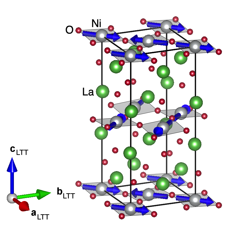
Figure 1: The low-temperature crystal and magnetic structure of La₂NiO₄ based on Ref. Rodriguez-Carvajal et al. (1991). Blue arrows denote the Ni spins. The unit cell in this figure is labeled with the $P4_{2}/ncm$ (LTT) space group with $a_{\mathrm{LTT}}=b_{\mathrm{LTT}}\approx 5.5$ Å and $c\approx 12.55$ Å. Shaded squares indicated the four planar-oxygen sites surrounding each Ni²⁺ ion and the buckling of the plane.

Previous inelastic neutron scattering (INS) Aeppli and Buttrey (1988); Nakajima et al. (1993) and resonant inelastic x-ray scattering (RIXS) Fabbris et al. (2017) studies show the existence of spin waves up to $\sim 120$ meV. A study Nakajima et al. (1993) of the spin-wave dispersion in the $(H,H,L)$-plane observed two distinct gapped modes corresponding to fluctuations in and out of the $ab$-plane. The gaps were assigned to single-ion anisotropy. The Heisenberg NN interaction was determined to be $J\approx 30$ meV. No out-of-plane, $\mathbf{c}$-axis, dispersion was observed implying $J_{\perp}/J<10^{-3}$ and making the magnetic excitations quasi-2D.

In this paper we present time-of-flight (ToF) INS data collected throughout the entire Brillouin zone and up to energy transfers of $\hslash\omega\approx 170$ meV on a high-quality single crystal of LNO. This enables us to resolve an anomalous high-$\hslash\omega$ spin-wave dispersion which resembles behavior observed in the $S=1/2$ SLAFM cuprate CFTD where it is assigned to quantum-dispersion-renormalization effects beyond linear-order spin-wave theory (Rønnow et al., 2001; Dalla Piazza et al., 2014; Christensen et al., 2007). In addition, we show that the spectral weights are well described by a LSWT+$1/S$ model if anisotropy, covalency effects and two-magnon excitations are considered.

II Experimental details

A LNO single crystal with a mass of $21.1$ g was grown by the floating-zone technique and annealed at $1173$ K in $5$% CO and $95$% CO₂ atmosphere to obtain the correct oxygen composition. A SQUID magnetometry measurement at 1 T shows a Néel temperature of $T_{N}(1\,\mathrm{T})\approx 320$ K and a structural and spin reorientation transition at 75 K. Thus, the oxygen excess $\delta$ in La₂NiO_4+δ is $\delta<0.007$ (Rodriguez-Carvajal et al., 1991; Buttrey et al., 1986).

The ToF INS experiments were performed at the MAPS instrument at the ISIS Neutron and Muon Source at the Rutherford Appleton Laboratory (Ewings et al., 2019; Hayden and Boothroyd, 2009) and the SEQUOIA instrument at the Spallation Neutron Source at the Oak Ridge National Laboratory (Granroth et al., 2010). Data were collected at $T=10$ K and $T=6$ K respectively. The sample was aligned with $(1\overline{1}0)$ vertically. All presented MAPS data are integrated over $L\in[-15,15]$ r.l.u. and all presented SEQUOIA data are integrated over $L\in[-10,10]$ r.l.u.

II.1 Crystallographic Notation

The low-temperature structure of LNO is the LTT $P4_{2}/ncm$ structure Rodriguez-Carvajal et al. (1991). This can be approximately described by the high-temperature tetragonal (HTT) $I4/mmm$ space group. We use the HTT conventional unit cell with $a=b=a_{\mathrm{HTT}}\approx 3.89$ Å and $c\approx 12.55$ Å to describe wave vectors in reciprocal space as $\mathbf{q}=H\mathbf{a}^{\star}+K\mathbf{b}^{\star}+L\mathbf{c}^{\star}\equiv(H,K,L)$ for the presentation of our data. For data integrated over $L$ and the spin wave theory we abbreviate to a square-lattice 2D-notation $(H,K)$. For a square-lattice the points $(H,K)$ and $(K,H)$ are equivalent.

II.2 Magnetic Structure

At low temperatures, the host lattice of the antiferromagnetism in near stoichiometric LNO is believed to be $P4_{2}/ncm$ or LTT. Samples with a similar composition to ours develop a ferromagnetic (FM) component (i.e. show canting of the ordered moments) and have anomalies in the intensity of the antiferromagnetic Bragg peak measured by neutron scattering on entering the LTT state at $T\approx 75$ K Yamada et al. (1992). Rodriguez-Carvajal et al. Rodriguez-Carvajal et al. (1991) (Table 4) show that only a magnetic structure belonging to the $\Gamma_{3g}$ irreducible representation of the $P4_{2}/ncm$ space group is consistent with this. We therefore assume that there is spin reorientation on entering the $P4_{2}/ncm$ structure and the antiferromagnetic structure is described by this magnetic mode as shown in Fig. 1. Note that this magnetic structure cannot be distinguished using diffraction from the $\Gamma_{4g}$ representation of the $Bmab$ space group proposed by Ref. Rodriguez-Carvajal et al. (1991) if two domains, rotated by 90^∘ around the $\mathbf{c}$-axis, of equal population are present. In the $P4_{2}/ncm$ space group, the local-point-group symmetry of the Ni²⁺ ions is $2/m$ and the moments are contained in the local mirror plane and point along the square diagonals of the LTT crystal structure such that the moments in adjacent layers are orthogonal as shown in Fig. 1. In relation to the HTT structure moments in the basal (middle) layer point almost along the $\mathbf{a}$ $(\mathbf{b})$ direction in HTT notation.

III Results

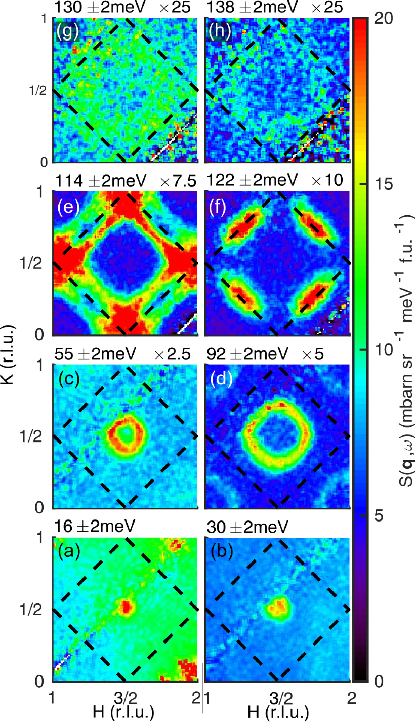
Figure 2: Representative constant-$\hbar\omega$ slices through the LNO data collected on SEQUOIA with $E_{i}=190$ meV. The circles and other structures in panels up to $\hbar\omega=122$ meV are mostly due to single-magnon scattering. For $\hbar\omega\geq 130$ meV two-magnon scattering is observed. The dashed lines are the mBZ boundaries.

The data are plotted and analyzed with the Horace package (Ewings et al., 2016). Fig. 2 shows representative slices through the data collected with an incident energy $E_{i}=190$ meV at the SEQUOIA instrument in terms of the scattering law $S(\mathbf{q},\omega)=\tfrac{k_{i}}{k_{f}}\tfrac{\mathrm{d}^{2}\sigma}{\mathrm{d}\Omega\mathrm{d}E^{\prime}}$. Data are normalized to absolute units via nuclear incoherent scattering from a vanadium standard, and are symmetrized about the $(H,H,0)$, $(H,\overline{H},0)$, and $(H,0,0)$ lines. The data collected at the MAPS instrument appear very similar. The slices in Fig. 2(a)-(d) show strong scattering as circles centered on (3/2,1/2), the center of an antiferromagnetic BZ. These are from one-magnon excitations, or spin waves. The scattering is consistent with spin gaps observed previously (Nakajima et al., 1993). Around 92 meV, spin-wave branches dispersing from reciprocal lattice points [e.g. (200)] become observable near the corners. In (e)-(f), lines of scattering parallel to the magnetic BZ (mBZ) boundaries (dashed lines) are the spin-wave branches originating from the (3/2,1/2) and (1,0)-type positions. The scattering in panels (g)-(h) is believed to be multi-magnon excitations. At higher $\hslash\omega$ the spin waves appear stronger first at the corners of the mBZ, and then at highest $\hslash\omega$ at the midpoints of the mBZ edges. This is unexpected for a classical NN Heisenberg SLAFM where no dispersion is expected along the mBZ boundaries. There, equal scattering, except for the magnetic form factor, is expected along the black dotted lines.

Our data are qualitatively consistent with a Néel SLAFM with single-ion anisotropy, significant multi-magnon scattering and an anomalous high-$\hslash\omega$ dispersion. For further analysis, a smooth function is fitted to a $\hbar\omega$-dependent cut at the ferromagnetic reciprocal-lattice position (1,0) and subtracted from all analyzed data. This removes most incoherent and multi-phonon background.

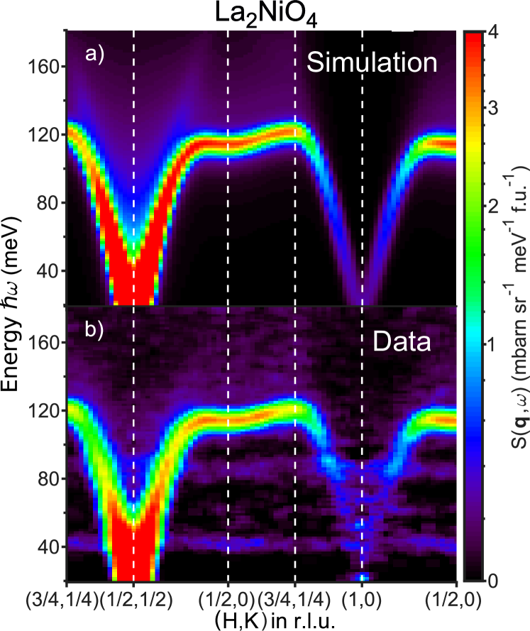
Figure 3: Magnetic excitations in La₂NiO₄. (a) Scattering function $S(\mathbf{q},\omega)$ simulated from Eqns. 5-7 convoluted with finite lifetime and resolution. (b) INS data collected with $E_{i}=260$ meV at SEQUOIA. A background consisting of a smooth interpolation of a $\mathbf{q}=(1,0)$ spectrum integrated over $L\in[-15,15]$ has been subtracted from each $\mathbf{q}$. A non-linear color-coded intensity scale is used to enhance the weak two-magnon scattering.

The calculated and measured intensities of the magnetic excitations after background subtraction are shown in Fig. 3(a,b). The multi-magnon scattering and anomalous dispersion are clearly visible at the mBZ boundary. The two, mostly dispersionless, lines at $\sim 42$ meV and $\sim 87$ meV are optical phonon modes.

One-dimensional (1D) cuts are taken through the data along high-symmetry lines marked in the inset of Fig. 4(b) to fit the data with the model described in the following section. The data sets from both instruments are individually fitted to determine the model parameters. Some representative cuts with fits are shown in Fig. 4(d).

IV Spin-wave model for a single NiO₂ plane

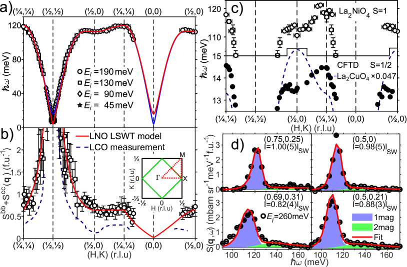
Figure 4: Results of the data fitting and comparison with similar compounds: (a) Spin wave dispersion sup in red (blue) for the in-plane (out-of-plane) mode with the peak positions from the MAPS data; (b) Amplitude of the spin-wave pole in units of spin (Multiply by $g^{2}\mu_{B}^{2}$ to get in units of $\mu^{2}_{B}$.) from the Horace (Ewings et al., 2016) fitting of Eqns. 5-6 to the MAPS data, LSWT prediction with $Z_{\textrm{co}}=0.78(6)$ (red) and absolute results from LCO with $Z_{\textrm{co}}=0.89(23)$ (Headings et al., 2010) for $Z_{d}(S=\tfrac{1}{2})=0.57$ (Canali and Wallin, 1993; Canali et al., 1992) (blue dashed); (c) MAPS data in comparison with CFTD (Rønnow et al., 2001) and LCO dispersion scaled by $J(\mathrm{CFTD})/Z_{c}J(\mathrm{LCO})=0.047$ (Headings et al., 2010) (blue dashed); It is noted that $(0,\tfrac{1}{2})$ is equivalent to $(\tfrac{1}{2},0)$; (d) Representative cuts through the SEQUOIA data fitted with one+two-magnon model with $\hslash\Gamma=1.5$ meV.

LNO is a Hubbard-Mott insulator, its magnetism is well described by an extended Heisenberg model with spin quantum number $S=1$ on the Ni²⁺ (3d⁸) sites with the orbital moments quenched by the octahedral-crystal-field environment of oxygen ions. We consider a single NiO₂ layer (the basal layer in Fig. 1) with the ordered moment along the $\mathbf{z}$-axis or $\mathbf{a}$ (See Sec. II.1). The spin Hamiltonian can be written as (Roger and Delrieu, 1989; Chubukov et al., 1992; Nakajima et al., 1993; Nolting and Ramakanth, 2009; Coldea et al., 2001; Marshall and Lovesey, 1971)

$$\mathcal{H} =\sum_{\langle i,j\rangle}J_{ij}\mathbf{S}_{i}\cdot\mathbf{S}_{j}\!+\!\sum_{i}\left[K_{c}\big{(}S^{y}_{i}\big{)}^{2}\!+\!K_{a}\big{(}S^{z}_{i}\big{)}^{2}\right]$$

$$+J^{\Box}\!\!\sum_{\langle i,j,k,l\rangle}[(\mathbf{S}_{i}\cdot\mathbf{S}_{j})(\mathbf{S}_{k}\cdot\mathbf{S}_{l})+(\mathbf{S}_{i}\cdot\mathbf{S}_{l})(\mathbf{S}_{k}\cdot\mathbf{S}_{j})$$

$$-(\mathbf{S}_{i}\cdot\mathbf{S}_{k})(\mathbf{S}_{j}\cdot\mathbf{S}_{l})],$$ (1)

where $J_{ij}$ represents the first to third NN Heisenberg exchange interactions $J$, $J^{\prime}$ and $J^{\prime\prime}$, $K_{a}\leq 0$ is an easy-axis anisotropy and $K_{c}\geq 0$ an out-of-plane hard-axis anisotropy. Here $(x,y,z)$ are along the HTT $(b,c,a)$ axes respectively (see Sec. II.1). The local-anisotropy terms are symmetry allowed in the $2/m$ local-point-group symmetry of the Ni²⁺ ions in the LTT structure (the local mirror plane is $ac$) and are attributed to higher-order effects of the local crystal field and spin-orbit coupling. A bilinear-biquadratic interaction, suggested for $S=1$, is neglected as it becomes indistinguishable from other interaction terms in the Néel state (Oitmaa and Hamer, 2013; Papanicolaou, 1988; Tóth et al., 2012). Also, an out-of-plane spin canting of 0.1^∘, assigned to a finite Dzyaloshinskii–Moriya interaction (DMI), has been observed Yamada et al. (1992). Although DMI can induce non-degenerate spin-wave modes the spin canting is too small to describe the previously reported gap size Nakajima et al. (1993); Toth and Lake (2015); Yamada et al. (1992) (see Ref. Nakajima et al. (1993) and Appendix X.4) and hence it is neglected in our analysis. The cyclic-term $J^{\Box}$ considered in LCO  (MacDonald et al., 1988, 1990; Klein and Seitz, 1973; Kato, 1949) is indistinguishable in LSWT from $J^{\prime}$ and is considered later (see also Appendix X.2).

The spin-wave excitations of the Hamiltonian are determined in the harmonic limit, commonly referred to as LSWT. For more details see Appendices X.2 and X.3. There are two distinct spin-wave modes for $K_{c}>0$ corresponding to spin fluctuations along $\mathbf{b}$ (in-plane) and $\mathbf{c}$ (out-of-plane) respectively. Their dispersion relations are given by $\hslash\omega_{\mathbf{q}}$ and $\hslash\omega_{\mathbf{q}}^{\prime}=\hslash\omega_{\mathbf{q}+\bm{\tau}_{\textrm{AF}}}$ respectively, where

$$\hslash\omega_{\mathbf{q}} =Z_{c}\sqrt{A_{\mathbf{q}}^{2}-B_{\mathbf{q}}^{2}},$$ (2)

$$A_{\mathbf{q}} =4S\left[-\frac{K_{a}}{2}+\frac{K_{c}}{4}+J-J^{\prime}(1-\nu_{h}\nu_{k})\right],$$ (3)

$$B_{\mathbf{q}} =4S\left[J\frac{\nu_{h}+\nu_{k}}{2}-\frac{K_{c}}{4}\right],$$ (4)

with $\nu_{\xi}\!=\!\cos(2\pi\xi)$ and $\bm{\tau}_{\textrm{AF}}=(1/2,1/2)$ the Néel-magnetic-structure propagation vector, expressed in reciprocal-lattice units of the HTT unit cell. $Z_{c}\approx 1.09$ is a spin-fluctuation correction factor which renormalizes the excitation energy (Igarashi, 1992; Singh, 1989). The Bogoliubov transformation parameters then yield the correlation (scattering) functions for the one- and two-magnon excitations in the $T\rightarrow 0$ limit (White et al., 1965; Heilmann et al., 1981; Ewings et al., 2008; Lorenzana et al., 2005; Coldea et al., 2003) (See Appendix X.2)

$$S^{bb}(\mathbf{q},\omega)\!= \frac{Z_{d}Z_{\textrm{co}}S}{2}\left|u_{\mathbf{q}}\!-\!v_{\mathbf{q}}\right|^{2}\delta(\hslash\omega\!-\!\hslash\omega_{\mathbf{q}})$$ (5)

$$S^{cc}(\mathbf{q},\omega)\!= \frac{Z_{d}Z_{\textrm{co}}S}{2}\left|u_{\mathbf{q}\!+\!\bm{\tau}_{\textrm{AF}}}\!+\!v_{\mathbf{q}\!+\!\bm{\tau}_{\textrm{AF}}}\right|^{2}\delta(\hslash\omega\!-\!\hslash\omega_{\mathbf{q}\!+\!\bm{\tau}_{\textrm{AF}}})$$ (6)

$$S^{aa}(\mathbf{q},\omega)\!= NZ_{\textrm{co}}^{2}(S\!-\!\Delta S)^{2}\delta(\hslash\omega)\delta(\mathbf{q}\!-\!\bm{\tau}_{\textrm{AF}}\!-\!\bm{\tau})+$$

$$\frac{Z_{2\rm{M}}Z_{\textrm{co}}}{2N} \sum_{\mathbf{q}_{1},\mathbf{q}_{2}}f(\mathbf{q}_{1},\mathbf{q}_{2})\delta(\hslash\omega\!-\!\hslash\omega_{\mathbf{q}_{1}}\!-\!\hslash\omega_{\mathbf{q}_{2}})\times$$

$$\delta(\mathbf{q}\!-\!\bm{\tau}_{\textrm{AF}}\!-\!\mathbf{q}_{1}\!-\!\mathbf{q}_{2}\!-\!\bm{\tau}),$$ (7)

where $u_{\mathbf{q}}=\cosh\theta_{\mathbf{q}}$, $v_{\mathbf{q}}=\sinh\theta_{\mathbf{q}}$, $\tanh(2\theta_{\mathbf{q}})=B_{\mathbf{q}}/A_{\mathbf{q}}$, $f(\mathbf{q}_{1},\mathbf{q}_{2})=\left|u_{\mathbf{q}_{1}}v_{\mathbf{q}_{2}}+u_{\mathbf{q}_{2}}v_{\mathbf{q}_{1}}\right|^{2}$. $N$ is the total number of spins in the lattice, $\bm{\tau}$ is a (HTT structural) reciprocal lattice vector, and $\Delta S=\langle v^{2}\rangle$ is the zero-point spin reduction, where $\langle...\rangle$ means the average over the full Brillouin zone. The first term in $S^{aa}$ (denoting fluctuations along the $\mathbf{a}$ axis) contains the elastic magnetic Bragg peak and the second term is the inelastic two-magnon continuum, with one of the two wave vectors in the sum restricted to one full Brillouin zone. The above dynamical correlations and the dispersion relation $\omega_{\mathbf{q}}$ have the translational periodicity of the full Brillouin zone.

The prefactor $Z_{d}$ is a one-magnon intensity renormalization factor due to higher order effects neglected at linear order in spin-wave theory, $Z_{2\rm{M}}$ is a corresponding factor for the two-magnon scattering. We have also included an additional factor $Z_{\textrm{co}}$ in Eqns. 5-7 to take account of covalency effects, $Z_{\textrm{co}}=1$ in the absence of these. For $K_{c}=0$, $Z_{d}=1-\Delta S/S$, and assuming $Z_{2\rm{M}}=1$, the total spin sum rule is satisfied such that elastic, one-magnon and two-magnon scattering integrated over all energies and a full Brillouin zone add up to $S(S+1)$ per spin, shared between the three contributions as $(S-\Delta S)^{2}$, $\left(S-\Delta S\right)(2\Delta S+1)$ and $\Delta S(\Delta S+1)$, respectively. To derive the above we have used the fact that $u$ is even and $v$ is odd with respect to a wave-vector shift by the magnetic propagation vector $\bm{\tau}_{\textrm{AF}}$, so the average $\langle uv\rangle=0$. For finite $K_{c}$, this is no longer the case and to satisfy the total sum rule one needs to use

$$Z_{d}=1-\frac{\Delta S}{S}-\frac{\langle uv\rangle^{2}}{S(2\Delta S+1)}$$ (8)

as the integrated two-magnon scattering becomes $\Delta S(\Delta S+1)+\langle uv\rangle^{2}$.

Significant two-magnon scattering is observed even in spin-5/2 systems. So we expect to see this also in the present $S=1$ system Huberman et al. (2005) and signatures are presented in Fig. 4d) and 2g) and h) as shown in Fig. 5b) and c), respectively. Eqn. 7 is evaluated on a three-dimensional grid ($\mathbf{q}_{2D},\hslash\omega)$ and then convolved with a $\mathbf{q}$-independent inverse lifetime of $\hslash\Gamma=$1.5 meV per excited magnon. To fit the data Eqns. 5-6 are added after lifetime broadening to the three-dimensional grid and these spin-spin correlation functions are then multiplied by the anisotropic magnetic form factor of the Ni²⁺ $e_{g}$-orbitals (Weiss and Freeman, 1959; Clementi and Roetti, 1974; Desclaux and Freeman, 1978; Freeman and Desclaux, 1979; Anderson et al., 2006). Deviations due to covalency are included through the factor $Z_{\mathrm{co}}$. Finally, these functions are convolved with the instrument resolution function by Tobyfit in the Horace package (Ewings et al., 2016). Simulations of $S^{aa}(\mathbf{q},\omega)$ without instrumental and lifetime broadening are shown in Fig. 5. The two-magnon term appears unusual due to the anisotropy gaps resulting in a ‘peak’ above $\hslash\omega_{\mathbf{q}}$ rather than a tail arising at $\hslash\omega_{\mathbf{q}}$. It is further observed that the instrument resolution dominates the broadening.

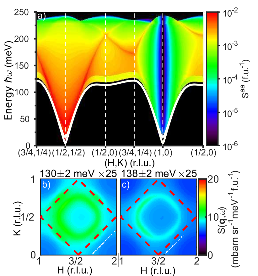
Figure 5: a) Simulation of two-magnon scattering using Eqn. 7. The solid white lines show the magnon dispersions $\hslash\omega_{\mathbf{q}}$ and $\hslash\omega_{\mathbf{q}+\bm{\tau}_{\textrm{AF}}}$. b,c) Simulations of $S(\mathbf{q},\omega)$ due to two-magnon scattering with an added constant background of $0.28$ or $0.24$ mb^-1sr^-1f.u.^-1, respectively. These closely resemble the slices in Fig. 2g) and h), respectively.

V Dispersion

In order to plot the dispersion, we fitted Gaussian functions to 1D cuts through the data to obtain the peak positions, plotted in Fig. 4(a). Constant-$\mathbf{q}$ cuts with $E_{i}=45$ meV at low-$\hslash\omega$ clearly show two distinct gapped spin-wave modes (not shown). The high-$\hslash\omega$ excitations show dispersion along the mBZ boundary. From the lower-$\hslash\omega$ data ($\leq 50$ meV) we can obtain an estimate of the $J\approx 29$ meV and the spin gaps at (1/2,1/2) $\Delta_{1}\!\approx\!4Z_{c}\sqrt{\!J(-K_{a})}\approx 5$ meV and $\Delta_{2}\approx\!4Z_{c}\sqrt{J(K_{c}\!-\!K_{a})}\approx 16$ meV are in good agreement with previous work (Nakajima et al., 1993). We mostly fixed $K_{a}$ (see Table 1) when fitting the whole dispersion curve below.

The high-$\hslash\omega$ dispersion cannot be described by $J$ only in LSTW but requires a finite $J^{\prime}$. The upturn from $\mathbf{q}=(1/2,0)$ to $\mathbf{q}=(1/4,1/4)$ can be described by an antiferromagnetic $J^{\prime}>0$ with $J^{\prime}\approx 5.8(3)\%$ of $J$ which yields, including the anisotropy, a difference of $\sim 6\%$ between $(1/2,0)$ and $(1/4,1/4)$. The $J^{\prime}>0$ describes the dispersion along the mBZ boundaries as well as the local dispersion minimum at $(1/2,0)$. Adding $J^{\prime\prime}$, described in Eqn. 12, does not improve the fitting, and is hence neglected from now on.

$J$	$J^{\prime}$	$J^{\prime\prime}$	$J^{\Box}$	$K_{a}$	$K_{c}$
(meV)	(meV)	(meV)	(meV)	(meV)	(meV)
29.02(8)	1.68(5)	0 (-)	0 (-)	-0.035(3)	0.443(11)
28.2(11)	1.3(5)	-0.2(3)	0 (-)	-0.04 (-)	0.46(2)
29.00(8)	1.67(5)	0 (-)	0 (-)	-0.04 (-)	0.445(11)
32.34(13)	0 (-)	0 (-)	-1.67(5)	-0.04(-)	0.445(11)

Table 1: Fitted Heisenberg coupling and anisotropy constants which determine the dispersion given in Eqn. 2. The rows describe different fitting models, the first row includes no $J^{\prime\prime}$, the second row includes all terms but with $K_{a}$ fixed and adapted from Ref. (Nakajima et al., 1993) and the third row excludes $J^{\prime\prime}$ and again uses the value from Ref. (Nakajima et al., 1993), for $K_{a}$. The forth row parameterizes the second row in terms of $J$ and $J^{\Box}$. Parameters marked $(-)$ are fixed during fitting.

La₂CuO₄ shows an inverted dispersion (with respect to LNO) along the mBZ boundary $[(0,1/2)-(1/4,1/4)]$ and $J^{\prime}<0$ (when $J^{\Box}=0$) (Coldea et al., 2001) (See Fig. 4(c)). The dispersion in LCO can be explained by higher-order terms in the $t/U$ expansion of the Hubbard model for hopping between Cu sites. This yields, terms in $J^{\Box}$, $J^{\prime}$ and $J^{\prime\prime}$ (MacDonald et al., 1988, 1990; Klein and Seitz, 1973; Takahashi, 1977). The term in $J^{\Box}$ has the same effect on the dispersion as $J^{\prime}$ in LSWT (see Eqn. 12) so cannot be distinguished from $J^{\prime}$.

The $S=3/2$ $3d$ square-lattice transition-metal-oxide AFM La₂CoO₄ (LCoO) has the same LTT structure as La₂NiO₄ and neutron scattering measurements of the magnon dispersion have also been carried out on this material Babkevich et al. (2010). The spin-wave excitations in LCoO also show dispersion along the mBZ with a minimum at ($1/2,0)$, as in LNO, but the effect is weaker in LCoO than in LNO. In Table 2 we compare the exchange couplings of LCO, LNO and LCoO. Both LNO and LCoO have $J^{\prime}>0$. Thus, the anomalous compound is LCO, which yields $J^{\prime}<0$ when fitted with $J^{\Box}=0$. The natural conclusion is that cyclic exchange is present in LCO, but negligible in LNO and LCoO which is consistent with the more substantial $t/U$ in LCO.

	$S$	$J$	$J^{\prime}$	$J^{\prime\prime}$	$J^{\Box}$
		(meV)	(meV)	(meV)	(meV)
La2CuO4 Headings et al. (2010)	1/2	114(2)	-12(2)	2.9 (2)	0(-)
La2CuO4, $t/U$ Headings et al. (2010)	1/2	143(2)	2.9 (2)	2.9 (2)	58(4)
La2NiO4	1	28.2(11)	1.3(5)	-0.2(3)	0(-)
La2CoO4 Babkevich et al. (2010)	3/2	9.69(2)	0.43(1)	0.12(2)	0(-)

Table 2: Comparison of exchange constants for square-lattice $3d$ transition-metal-oxide AFMs. Here $S$ is the spin and $t/U$ indicates results from fitting with the extended $t/U$-expansion (MacDonald et al., 1988, 1990; Klein and Seitz, 1973; Takahashi, 1977).

As shown in Fig. 4(c) the high-$\hslash\omega$ dispersion in LNO however closely resembles the dispersion in the $S=1/2$ SLAFM copper deuteroformate tetradeuterate (CFTD) (Rønnow et al., 2001; Dalla Piazza et al., 2014; Christensen et al., 2007) as well as similar compounds such as Cu(pyrazine)₂(ClO₄)₂ (Tsyrulin et al., 2009, 2010), and CuF₂(H₂O)₂(pyrazine) (Wang et al., 2012). In these compounds the dispersion along the mBZ is explained by quantum effects which renormalize the dispersion. The dispersion in $S=$1/2 SLAFMs is predicted by various theoretical calculations. Although all models predict a dispersion on the mBZ boundary they disagree over the magnitude of the dispersion and its origin. To our knowledge no calculations are available at the time of the submission for $S=$1 SLAFMs but from the Holstein-Primakoff transformation a suppression of quantum effects by at least a factor of two from $S=$1/2 to $S=$1 systems is predicted (Verresen et al., 2018).

VI Spectral weight

The 1D cuts, taken from the MAPS instrument data, are used to fit the overall spectral weights due to the better resolution at low $\hslash\omega$. The cuts are fitted with the intensities calculated from Eqns. 5-6 convolved with a $\mathbf{q}$-independent inverse lifetime $\Gamma$. A linear function is added to remove multi-magnon scattering and a $\mathbf{q}$-dependent background. The fitted one-magnon spectral weights throughout the lattice BZ are depicted in Fig. 4(b). The $\mathbf{q}$-dependence of the one-magnon spectral weights is qualitatively well described by the LSWT model. Small deviations arise near the antiferromagnetic BZ center. Firstly, because the anisotropy prevents the divergence of the spectral weight there, and secondly, the fitting is hindered by contamination from the magnetic Bragg peak and the multi-magnon scattering. Utilizing the Hamiltonian parameters determined from the dispersion relations we find $\Delta S=0.188(1)$ and $\langle uv\rangle=-0.017(1)$, yielding $Z_{d}\approx 0.812(1)$. A fit of the high-$\hslash\omega$ one-magnon excitations using Eqns. 5-7, with $Z_{d}\approx 0.812(1)$, the SEQUOIA data yields $Z_{\textrm{co}}=0.78(6)$. The $Z_{d}$ follows from $\Delta S=0.188(1)$ and $\langle uv\rangle=-0.017(1)$, therein derived from the Hamiltonian parameters of the fitted dispersion relation. We believe $Z_{\textrm{co}}<1$ because there is a reduction of the ordered Ni²⁺ moment due to oxygen covalency effects as observed in neutron diffraction Wang et al. (1991, 1992); Lander et al. (1989).

In the related spin-1/2 compounds LCO and CFTD anomalous scattering is observed near (1/2,0) and equivalent (0,1/2) point. To study if such scattering also arises in LNO the one+two-magnon model is fitted to 59 constant-$\mathbf{q}$ cuts through the high-$\hslash\omega$ excitations in the SEQUOIA data. The model includes $Z_{\mathrm{co}}$ and the subsequent analysis focuses particularly on the comparison of (1/4,1/4) and the anomalous (1/2,0) point. All cuts are fitted with a small individual constant background term to account for $\mathbf{q}$-dependent variations in the background. Some representative fits are shown in Fig. 4(d) where $\Gamma=1.5$ meV and the fits are unchanged for smaller $\Gamma$ values.

As shown in Fig. 4(d), the model gives a good description of peak shapes and continua and, further, of the relative intensities of one- and two-magnon spectral weights. The calculated spectral weights also agree quantitatively well with the measured spectral weights after re-scaling for $Z_{\mathrm{co}}$. Moreover, the model including $Z_{\mathrm{co}}$ gives a good description along all high-symmetry directions as shown in Fig. 3(a) and (b).

In contrast to the $S=1/2$ compounds CFTD (Rønnow et al., 2001; Dalla Piazza et al., 2014; Christensen et al., 2007) and LCO (Headings et al., 2010), in LNO neither the reduced one-magnon spectral weight (see Fig. 4(b) nor the enhanced multi-magnon spectral weight is observed at (1/2,0) within the statistical limitations.

VII Discussion

In the preceding sections we have seen that although aspects of the magnetic excitations of LNO are qualitatively described by a simple linear-spin-wave theory with two-magnon scattering, the intensity and dispersion show some significant deviations. The measured spin-wave dispersion is well described by an anisotropic semi-classical NN Heisenberg AFM below $\sim$100 meV. This theory also qualitatively describes the two-magnon excitations observed for $\hslash\omega\approx 130$ meV. Two aspects of the excitations that are not well described by LSWT are the overall intensity of the excitations and the dispersion of the high-$\hslash\omega$ excitations.

The overall intensity of the excitations is determined by the absolute normalization of the measured signal and yields a scaling factor of $Z_{\textrm{co}}=0.78(6)$ through Eqns. 5-6 when the quantum renormalization factor $Z_{d}$ is taken into account. The most likely explanation for the difference from $Z_{\textrm{co}}=1$ are the covalency effects Wang et al. (1991, 1992); Lander et al. (1989) present in nickel oxides. This results in some of the ordered and fluctuating magnetic moments residing on the oxygen atoms, reducing the signal seen in the present experiment.

We also observe a deviation from the predictions of LSWT for a NN SLAFM in the form of significant dispersion along the mBZ boundaries. The dispersion indicates the presence of longer-ranged exchange interactions. The structurally related compound LCO also shows dispersion along the mBZ boundaries but with the opposite sense (Coldea et al., 2001). In the case of LCO, the dispersion is due to the substantial $t/U\approx 0.11$ resulting in a substantial ferromagnetic next-NN exchange $J^{\prime}<0$ in superexchange theory (MacDonald et al., 1988, 1990; Klein and Seitz, 1973; Takahashi, 1977). Such a mechanism cannot explain the antiferromagnetic $J^{\prime}>0$ observed in LNO and LCoO. An anisotropy in $J$ as origin of the high-$\hslash\omega$ dispersion is also excluded as this would imply two distinct high-$\hslash\omega$ spin-wave modes with differing dispersion, as shown in Ref. (Koshibae et al., 1994).

Thus, our observation of a downward dispersion from (1/4,1/4) to (1/2,0) seems to have two possible explanations. Either further-NN superexchange in La₂NiO₄ yields an antiferromagnetic $J^{\prime}$ or the quantum renormalization of the spin-wave dispersion proposed for the $S=1/2$ NN SLAFMs Rønnow et al. (2001); Dalla Piazza et al. (2014); Christensen et al. (2007); Tsyrulin et al. (2009, 2010); Wang et al. (2012) is also present in $S=1$ systems. Testing the first proposal will require detailed electronic structure calculations of the next-NN superexchange in La₂NiO₄. This is beyond the scope of this present study. However, we note that $t/U$ is smaller in La₂NiO₄ and that other pathways such as Ni-O-O-Ni with direct overlap between the oxygens may be more important in La₂NiO₄ than La₂CuO₄ Annett et al. (1989). Thus, the $t^{\prime}$ hopping involving these oxygens could yield an antiferromagnetic $J^{\prime}$.

A second proposal, that the downward dispersion is due to a renormalization of the spin wave energies, is supported by the similarity to $S=$1/2 SLAFMs: CFTD (Rønnow et al., 2001; Dalla Piazza et al., 2014; Christensen et al., 2007), Cu(pyrazine)₂(ClO₄)₂ (Tsyrulin et al., 2009, 2010) and CuF₂(H₂O)₂(pyrazine) (Wang et al., 2012). Furthermore, it resembles the dispersion predicted by various theoretical models for $S=$1/2 NN SLAFMs. These models suggest that quantum effects lead to an anomaly in the dispersion at (1/2,0). The techniques used in the models are series expansions (SE) of the NN Heisenberg-Ising model (Singh and Gelfand, 1995; Zheng et al., 2005), quantum Monte-Carlo simulations (Sandvik and Singh, 2001; Shao et al., 2017), exact diagonalization (Lüscher and Läuchli, 2009), continuous similarity transformations (Powalski et al., 2018, 2015) and density matrix renormalization group (DMRG) simulations (Verresen et al., 2018).

In CFTD (Rønnow et al., 2001; Dalla Piazza et al., 2014; Christensen et al., 2007) and LCO (Headings et al., 2010), the one-magnon spectral weight is suppressed near (1/2,0) relative to LSWT and a strong continuum with longitudinal and transverse character is observed. LSWT predicts the same one-magnon spectral weight along the entire mBZ boundary. However, some of the other models for $S=$1/2 quantum SLAFM mentioned above predict the suppressed spectral weight and continuum near $(1/2,0)$. We find no evidence for a wave-vector-dependent variation of the one-magnon spectral weight or continuum at (1/2,0) in LNO.

VIII Conclusion

Our results show that magnetic excitations in La₂NiO₄ are not described by a simple classical ($S\rightarrow\infty$) Heisenberg model with only nearest-neighbor interactions. The energy of the spin waves disperses along the antiferromagnetic Brillouin zone boundary from (1/4,1/4) to a minimum at (1/2,0). This is in the opposite sense to that in the $S=1/2$ system La₂CuO₄, but the same sense as in other $S=1/2$ systems with smaller $t/U$ and the isostructural $S=3/2$ compound La₂CoO₄. The origin of the dispersion in La₂NiO₄ is unclear. It may be due to a quantum renormalization of the spin-wave energies or an antiferromagnetic second-nearest-neighbor superexchange. The overall intensity of the spin wave excitations is suppressed relative to linear spin-wave theory, probably due to covalency effects.

IX Acknowledgments

The authors would like to thank Ruben Verresen, Roderich Moessner and James Annett for useful discussions. A.N.P. and S.M.H acknowledge funding and support from the Engineering and Physical Sciences Research Council (EPSRC) under Grant Nos. EP/L015544/1 and EP/R011141/1. Beamtime at ISIS and SNS were provided under proposals RB920380 Hayden and Boothroyd (2009) and 26529.1 respectively. A portion of this research used resources at the Spallation Neutron Source, a DOE Office of Science User Facility operated by the Oak Ridge National Laboratory. A.N.P. acknowledges support from the U.S. Department of Energy, Office of Science, Basic Energy Sciences, Materials Sciences and Engineering Division, under Contract No. DE-AC02-76SF00515. R.C. acknowledges support from the European Research Council under the European Union’s Horizon 2020 Research and Innovation Programme Grant Agreement No.: 788814 (EQFT).

X Appendix

X.1 Neutron Scattering and Dynamic Correlation Functions

Inelastic neutron scattering measures dynamic spin-spin correlation functions defined as

$$S^{\alpha\beta}(\mathbf{q},\omega)=\frac{1}{2\pi\hslash}\int_{-\infty}^{\infty}e^{-i\omega t}\langle S_{\mathbf{q}}^{\alpha}(0)S_{\mathbf{-q}}^{\beta}(t)\rangle\,\text{d}t,$$ (9)

where $\mathbf{S}_{\mathbf{q}}$ is the Fourier transformed spin operator Marshall and Lovesey (1971); Boothroyd (2020) (Multiply by $g^{2}\mu_{B}^{2}$ to get in units of $\mu^{2}_{B}$). Our model spin-wave calculations compute $S^{\alpha\beta}(\mathbf{q},\omega)$ which is diagonal in our case. In the dipole approximation the magnetic inelastic neutron scattering cross section is given by

$$\dfrac{\text{d}^{2}\sigma}{\text{d}\Omega\text{d}E^{\prime}}= \ \dfrac{k_{f}}{k_{i}}S(\mathbf{q},\omega)$$

$$= \ \dfrac{k_{f}}{k_{i}}\left(\dfrac{\gamma r_{e}}{2\mu_{B}}\right)^{2}|F(\mathbf{q})|^{2}e^{-2W}$$

$$\ \ \times\sum_{\alpha\beta}\left(\delta_{\alpha\beta}-\frac{q_{\alpha}q_{\beta}}{q^{2}}\right)g^{2}\mu_{B}^{2}\,S^{\alpha\beta}(\mathbf{q},\omega),$$ (10)

where $g\approx 2$, $e^{-2W}\approx 1$ for low temperatures, $F(\mathbf{q})$ is the magnetic form factor, $\mu_{B}$ is the Bohr magneton, and $(\gamma r_{e}/2)^{2}$=72.4 mb.

While the model is derived for the basal NiO₂ layer in Fig. 1 with the spins aligned along the HTT $\mathbf{a}$-axis, $S^{aa}$ and $S^{bb}$ for neighboring NiO₂ planes in the LTT structure are related by a $90^{\circ}$ rotation around $\mathbf{c}$. This implies that in successive planes the fluctuations along the HTT $\mathbf{a}$- and $\mathbf{b}$-axes are interchanged. In the analysis this is considered by averaging the polarization factor over both axes.

Furthermore, although $S(\mathbf{q},\omega)$ is averaged over a range in $L$ by utilizing the HORACE Ewings et al. (2016) package the $\mathbf{q}$-vectors of the averaged pixels (neutrons) are retained and are then included in the calculations of Eqn. X.1. It is then averaged over the calculated values of $S(\mathbf{q},\omega)$. This accounts for the $\mathbf{q}$ dependence of the polarization factor and the magnetic form factor. For more details see Ref. Ewings et al. (2016) and HORACE documentation.

X.2 Derivation of Correlation Functions using Rotating Reference Frame

Here we summarize the derivations of the dynamical correlations (included two-magnon correlations) within linear spin-wave theory for a square-lattice spin Hamiltonian appropriate for the $S$=1 Ni²⁺ layers in La₂NiO₄ as given in Eqn. 1 with a collinear two-sublattice Néel magnetic structure. To the best of our knowledge the formulas have not been reported before for the Hamiltonian Eqn. 1 with the anisotropy terms included here.

It is convenient to transform the Hamiltonian to a rotating reference frame Coldea et al. (2003) where the local $xyz$ spin axes at every site are defined such that $\mathbf{z}$ is along the local ordered spin direction. In this frame the ground state is ferromagnetic and the magnetic unit cell is the same as the structural primitive unit cell (one spin per cell). This can be achieved by labelling the spin axes on the Néel A sublattice (which contains the origin) with ordered spins along the $+a$ axis as ($x,y,z$) along ($b,c,a$) and for the B sublattice with spins along $-a$ as ($x,y,z$) along ($b,-c,-a$), so at a general site $\mathbf{r}$ the spin components are given by $S^{x}_{\mathbf{r}}=S^{b}_{\mathbf{r}}$, $S^{y}_{\mathbf{r}}=-S^{a}_{\mathbf{r}}\sin(\bm{\tau}_{\textrm{AF}}\cdot\mathbf{r})+S^{c}_{\mathbf{r}}\cos(\bm{\tau}_{\textrm{AF}}\cdot\mathbf{r})$ and $S^{z}_{\mathbf{r}}=S^{a}_{\mathbf{r}}\cos(\bm{\tau}_{\textrm{AF}}\cdot\mathbf{r})+S^{c}_{\mathbf{r}}\sin(\bm{\tau}_{\textrm{AF}}\cdot\mathbf{r})$ with $\bm{\tau}_{\textrm{AF}}=(1/2,1/2)$ the Néel magnetic structure propagation vector, expressed in reciprocal lattice units of the structural HTT cell. Here ($S_{\mathbf{r}}^{a},S_{\mathbf{r}}^{b},S_{\mathbf{r}}^{c}$) are the spin components along the crystallographic HTT axes. In the rotating frame the spin-wave Hamiltonian to quadratic order is obtained as,

$${\cal H}_{\rm rot}=\frac{1}{2}\sum_{\mathbf{q}}\left[\begin{array}[]{cc}a^{{\dagger}}_{\mathbf{q}}&a_{-\mathbf{q}}\end{array}\right]\left[\begin{array}[]{cc}A_{\mathbf{q}}&B_{\mathbf{q}}\\ B_{\mathbf{q}}&A_{\mathbf{q}}\end{array}\right]\left[\begin{array}[]{l}a_{\mathbf{q}}\\ a_{-\mathbf{q}}^{{\dagger}}\end{array}\right],$$ (11)

where the sum extends over all wave vectors $\mathbf{q}$ in the full (structural) Brillouin zone and $a_{\mathbf{q}}^{{\dagger}}$ is the Fourier transformed spin creation operator. Here (including the cyclic exchange) we have,

$$A_{\mathbf{q}} =4S\bigg{[}-\frac{K_{a}}{2}+\frac{K_{c}}{4}+(J-2S^{2}J^{\Box})$$

$$-(J^{\prime}-S^{2}J^{\Box})(1-\nu_{h}\nu_{k})-J^{\prime\prime}(2-\nu_{h}^{2}-\nu_{k}^{2})\bigg{]}$$

$$B_{\mathbf{q}} =4S\left[(J-2S^{2}J^{\Box})\left(\frac{\nu_{h}+\nu_{k}}{2}\right)-\frac{K_{c}}{4}\right],$$ (12)

with $\nu_{\xi}=\cos(2\pi\xi)$. The $2\times 2$ Hamiltonian matrix in Eqn. 11 can be brought to diagonal form using a Bogoliubov basis transformation,

$$\left[\begin{array}[]{l}a_{\mathbf{q}}\\ a_{-\mathbf{q}}^{{\dagger}}\end{array}\right]=\left[\begin{array}[]{rr}u_{\mathbf{q}}&-v_{\mathbf{q}}\\ -v_{\mathbf{q}}&u_{\mathbf{q}}\end{array}\right]\left[\begin{array}[]{l}\alpha_{\mathbf{q}}\\ \alpha_{-\mathbf{q}}^{{\dagger}}\end{array}\right],$$ (13)

where $\alpha_{\mathbf{q}}^{{\dagger}}$ creates a spin wave with dispersion $\hslash\omega_{\mathbf{q}}=Z_{c}\sqrt{A_{\mathbf{q}}^{2}-B_{\mathbf{q}}^{2}}$, $u_{\mathbf{q}}=\cosh\theta_{\mathbf{q}}$, $v_{\mathbf{q}}=\sinh\theta_{\mathbf{q}}$, and $\tanh(2\theta_{\mathbf{q}})=B_{\mathbf{q}}/A_{\mathbf{q}}$. Here $Z_{c}$ is a dispersion renormalization factor due to higher order effects neglected at linear order in spin-wave theory. The dynamical correlations in the rotating frame (at zero temperature) are obtained as

$$S^{xx}(\mathbf{q},\omega) =Z_{d}\frac{S}{2}\left|u_{\mathbf{q}}-v_{\mathbf{q}}\right|^{2}\delta(\hslash\omega-\hslash\omega_{\mathbf{q}})$$

$$=Z_{d}\frac{S}{2}\sqrt{\frac{A_{\mathbf{q}}-B_{\mathbf{q}}}{A_{\mathbf{q}}+B_{\mathbf{q}}}}\delta(\hslash\omega-\hslash\omega_{\mathbf{q}})$$ (14)

$$S^{yy}(\mathbf{q},\omega) =Z_{d}\frac{S}{2}\left|u_{\mathbf{q}}+v_{\mathbf{q}}\right|^{2}\delta(\hslash\omega-\hslash\omega_{\mathbf{q}})$$

$$=Z_{d}\frac{S}{2}\sqrt{\frac{A_{\mathbf{q}}+B_{\mathbf{q}}}{A_{\mathbf{q}}-B_{\mathbf{q}}}}\delta(\hslash\omega-\hslash\omega_{\mathbf{q}})$$ (15)

$$S^{zz}(\mathbf{q},\omega) =N(S-\Delta S)^{2}\delta(\hslash\omega)\delta(\mathbf{q}-\bm{\tau})+$$

$$\ \ \ \ \frac{Z_{2\rm{M}}}{2N}\sum_{\mathbf{q}_{1},\mathbf{q}_{2}}f(\mathbf{q}_{1},\mathbf{q}_{2})\delta(\hslash\omega-\hslash\omega_{\mathbf{q}_{1}}-\hslash\omega_{\mathbf{q}_{2}})$$

$$\ \ \ \ \ \ \ \ \ \ \ \ \ \ \ \ \ \times\delta(\mathbf{q}-\mathbf{q}_{1}-\mathbf{q}_{2}-\bm{\tau}).$$ (16)

The dynamical correlations in the original (fixed) reference frame (Eqns. 5-7) are obtained through Fourier transformation, such that $S^{bb}\equiv S^{xx}$ whereas $S^{aa}(\mathbf{q},\omega)=S^{zz}(\mathbf{q}+\bm{\tau}_{\textrm{AF}},\omega)$ and $S^{cc}(\mathbf{q},\omega)=S^{yy}(\mathbf{q}+\bm{\tau}_{\textrm{AF}},\omega)$, i.e. the latter two correlation functions are momentum shifted by $\bm{\tau}_{\textrm{AF}}$. In obtaining Eqns. 5-7 we have used the fact that $2\bm{\tau}_{\textrm{AF}}$ is a vector of the reciprocal lattice of the HTT structural cell, so wavevectors $\mathbf{q}-\bm{\tau}_{\textrm{AF}}$ and $\mathbf{q}+\bm{\tau}_{\textrm{AF}}$ are equivalent by reciprocal space translational symmetry.

The in-plane (along $\mathbf{b}$) spin correlations shows a magnon mode with dispersion $\omega_{\mathbf{q}}$ (red line in Fig. 4(a)) with the gap

$$\Delta_{1} =4Z_{c}S\sqrt{\left(2J-\frac{K_{a}}{2}+\frac{K_{c}}{2}\right)\frac{-K_{a}}{2}}$$

$$\approx 4Z_{c}S\sqrt{J(-K_{a})}$$ (17)

and strong intensity above the antiferromagnetic Bragg peaks at $\bm{\tau}+\bm{\tau}_{\textrm{AF}}$, and the larger gap

$$\Delta_{2} =4S\sqrt{\left(2J-\frac{K_{a}}{2}\right)\left(\frac{-K_{a}}{2}+\frac{K_{c}}{2}\right)}$$

$$\approx 4Z_{c}S\sqrt{J(K_{c}-K_{a})}$$ (18)

and weak intensity at $\bm{\tau}$. The out-of-plane correlations (along $\mathbf{c}$) will show the wavevector-shifted dispersion $\omega^{\prime}_{\mathbf{q}}=\omega_{\mathbf{q}+\bm{\tau}_{\textrm{AF}}}$ (blue line in Fig. 4(a)) with reversed gaps compared to $\omega_{\mathbf{q}}$, i.e. gap $\Delta_{1}$ at $\bm{\tau}$ and $\Delta_{2}$ at $\bm{\tau}+\bm{\tau}_{\textrm{AF}}$. The longitudinal correlations (along $a$) will show the elastic magnetic Bragg peaks at $\bm{\tau}+\bm{\tau}_{\textrm{AF}}$ and a two-magnon continuum, with a gap of $\Delta_{1}+\Delta_{2}$ at $\bm{\tau}$ and onsets with gaps at $2\Delta_{1}$ and $2\Delta_{2}$ at $\bm{\tau}+\bm{\tau}_{\textrm{AF}}$.

X.3 Derivation of Correlation Functions using Antiferromagnetic Unit Cell

The dynamical correlation functions, derived in Appendix X.2, can also be derived in the antiferromagnetic unit cell. Utilizing this unit cell implies a doubling of the number of Ni²⁺ ions per unit cell and thus, an effective doubling of the spin-wave modes but does not require the transformation of the Hamiltonian to a rotating reference frame. The notations used in this section are the same as in Appendix X.2.

For the antiferromagnetic unit cell the spin-wave Hamiltonian to quadratic order can be written as

$${\cal H}\!=\!\!\frac{1}{2}\!\!\sum_{\mathbf{q}}\!\!\left[\!\!\begin{array}[]{c}a^{{\dagger}}_{\mathbf{q}}\\ b_{\mathbf{q}}\\ a_{\mathbf{-q}}\\ b^{{\dagger}}_{\mathbf{-q}}\!\end{array}\!\!\right]^{\!\!T}\!\!\left[\!\!\begin{array}[]{cccc}A_{\mathbf{q}}&B^{\prime}_{\mathbf{q}}&-SK_{c}&0\\ B^{\prime}_{\mathbf{q}}&A_{\mathbf{q}}&0&-SK_{c}\\ -SK_{c}&0&A_{\mathbf{q}}&B^{\prime}_{\mathbf{q}}\\ 0&-SK_{c}&B^{\prime}_{\mathbf{q}}&A_{\mathbf{q}}\\ \end{array}\!\!\right]\!\!\!\left[\!\!\begin{array}[]{c}a_{\mathbf{q}}\\ b^{{\dagger}}_{\mathbf{q}}\\ a^{{\dagger}}_{-\mathbf{q}}\\ b_{-\mathbf{q}}\end{array}\!\!\right],$$ (31)

where $B^{\prime}_{\mathbf{q}}=B_{\mathbf{q}}+SK_{c}$, $b^{{\dagger}}$ is the local spin deviation creation operator on the B sublattice, the sum extends over all wave vectors in the mBZ and $A_{\mathbf{q}}$, $B_{\mathbf{q}}$ are the same as in Eqn. 2. As can be seen, there are two flavors of operators. This 4 × 4 Hamiltonian matrix again can be brought to diagonal form using the following Bogoliubov basis transformation including two flavors of new spin wave creation (annihilation) operators, corresponding to spin-wave modes polarized along $\mathbf{b}$ and $\mathbf{c}$,

$$\left[\!\!\begin{array}[]{l}a_{\mathbf{q}}\\ b_{\mathbf{q}}^{{\dagger}}\\ a_{-\mathbf{q}}^{{\dagger}}\\ b_{-\mathbf{q}}\end{array}\!\!\right]=\frac{1}{\sqrt{2}}\!\!\left[\begin{array}[]{rrrr}u_{\mathbf{q}}&-v^{\prime}_{\mathbf{q}}&-v_{\mathbf{q}}&-u^{\prime}_{\mathbf{q}}\\ -v_{\mathbf{q}}&u^{\prime}_{\mathbf{q}}&u_{\mathbf{q}}&v^{\prime}_{\mathbf{q}}\\ -v_{\mathbf{q}}&-u^{\prime}_{\mathbf{q}}&u_{\mathbf{q}}&-v^{\prime}_{\mathbf{q}}\\ u_{\mathbf{q}}&v^{\prime}_{\mathbf{q}}&-v_{\mathbf{q}}&u^{\prime}_{\mathbf{q}}\end{array}\right]\left[\!\!\begin{array}[]{l}\alpha_{\mathbf{q}}\\ \beta_{\mathbf{q}}^{{\dagger}}\\ \alpha_{-\mathbf{q}}^{{\dagger}}\\ \beta_{-\mathbf{q}}\end{array}\!\!\right],$$ (32)

The transformation thus yields two sets of terms, $u_{\mathbf{q}}$, $v_{\mathbf{q}}$ and $\omega_{\mathbf{q}}$ and $u_{\mathbf{q}}^{\prime}=\cosh\theta_{\mathbf{q}}^{\prime}$, $v_{\mathbf{q}}^{\prime}=\sinh\theta_{\mathbf{q}}^{\prime}$ and $\omega_{\mathbf{q}}^{\prime}$ with,

$$\tanh(2\theta_{\mathbf{q}}) =\frac{B^{\prime}_{\mathbf{q}}-SK_{c}}{A_{\mathbf{q}}}=\frac{B_{\mathbf{q}}}{A_{\mathbf{q}}},$$ (33)

$$\tanh(2\theta^{\prime}_{\mathbf{q}}) =\frac{B^{\prime}_{\mathbf{q}}+SK_{c}}{A_{\mathbf{q}}}$$

$$=-\frac{B_{\mathbf{q}+\bm{\tau}_{\mathrm{AF}}}}{A_{\mathbf{q}+\bm{\tau}_{\mathrm{AF}}}}\ \ =-\tanh(2\theta_{\mathbf{q}+\bm{\tau}_{\mathrm{AF}}}),$$

and

$$\hslash\omega_{\mathbf{q}} =Z_{c}\sqrt{A_{\mathbf{q}}^{2}-(B^{\prime}_{\mathbf{q}}-SK_{c})^{2}}=Z_{c}\sqrt{A_{\mathbf{q}}^{2}-B_{\mathbf{q}}^{2}},$$ (34)

$$\hslash\omega_{\mathbf{q}}^{\prime} =Z_{c}\sqrt{A_{\mathbf{q}}^{2}-(B^{\prime}_{\mathbf{q}}+SK_{c})^{2}}$$

$$=Z_{c}\sqrt{A_{\mathbf{q+\bm{\tau}_{\mathrm{AF}}}}^{2}-B_{\mathbf{q}+\bm{\tau}_{\mathrm{AF}}}^{2}}\ \ \ \,=\hslash\omega_{\mathbf{q}+\bm{\tau}_{\mathrm{AF}}}.$$

Here we again use the fact that $2\bm{\tau}_{\textrm{AF}}$ is a reciprocal lattice vector.

The correlations functions $S^{bb}$ and $S^{cc}$ follow as,

$$S^{bb}(\mathbf{q},\omega)\!= \frac{Z_{d}S}{2}\left|u_{\mathbf{q}}\!-\!v_{\mathbf{q}}\right|^{2}\delta(\hslash\omega\!-\!\hslash\omega_{\mathbf{q}})$$ (35)

$$S^{cc}(\mathbf{q},\omega)\!= \frac{Z_{d}S}{2}\left|u^{\prime}_{\mathbf{q}}\!-\!v^{\prime}_{\mathbf{q}}\right|^{2}\delta(\hslash\omega\!-\!\hslash\omega_{\mathbf{q}}^{\prime})$$ (36)

$$= \frac{Z_{d}S}{2}\left|u_{\mathbf{q}+\bm{\tau}_{\mathrm{AF}}}\!+\!v_{\mathbf{q}+\bm{\tau}_{\mathrm{AF}}}\right|^{2}\delta(\hslash\omega\!+\!\hslash\omega_{\mathbf{q}+\bm{\tau}_{\mathrm{AF}}}).$$

Using the relations between $\tanh(2\theta_{\mathbf{q}})$ and $\tanh(2\theta^{\prime}_{\mathbf{q}})$ through the translation by $\bm{\tau}_{\mathrm{AF}}$ from Appendix X.2, the Eqns. 35-36 can be written as Eqns. 5-6 and thus, yield the same results as the rotating frame method.

The longitudinal dynamical correlations take the form,

$$S^{aa}(\mathbf{q},\omega) =N(S-\Delta S)^{2}\delta(\hslash\omega)\delta(\mathbf{q}-\bm{\tau}-\bm{\tau}_{\mathrm{AF}})+$$

$$\frac{Z_{2\rm{M}}}{2N} \sum_{\mathbf{q}_{1},\mathbf{q}_{2}}f^{\prime}(\mathbf{q}_{1},\mathbf{q}_{2})\delta(\hslash\omega-\hslash\omega_{\mathbf{q}_{1}}-\hslash\omega_{\mathbf{q}_{2}}^{\prime})\times$$

$$\delta(\mathbf{q}-\mathbf{q}_{1}-\mathbf{q}_{2}-\bm{\tau}),$$ (37)

where $f^{\prime}(\mathbf{q}_{1},\mathbf{q}_{2})=\left|v_{\mathbf{q}_{1}}u^{\prime}_{\mathbf{q}_{2}}-u_{\mathbf{q}_{1}}v^{\prime}_{\mathbf{q}_{2}}\right|^{2}$. Using the transformations relations, we find that,

$$f^{\prime}(\mathbf{q}_{1},\mathbf{q}_{2}) =\left|v_{\mathbf{q}_{1}}u^{\prime}_{\mathbf{q}_{2}}-u_{\mathbf{q}_{1}}v^{\prime}_{\mathbf{q}_{2}}\right|^{2}$$

$$=\left|v_{\mathbf{q}_{1}}u_{\mathbf{q}_{2}+\bm{\tau}_{\textrm{AF}}}+u_{\mathbf{q}_{1}}v_{\mathbf{q}_{2}+\bm{\tau}_{\textrm{AF}}}\right|^{2}$$

$$=f(\mathbf{q}_{1},\mathbf{q}_{2}+\bm{\tau}_{\textrm{AF}}),$$ (38)

Thus, we can transform Eqn. 37 to yield Eqn. 7. In the antiferromagnetic unit cell description the two spin-wave modes appear mixed in the two-magnon scattering and applying the shift by $\bm{\tau}_{\textrm{AF}}$ effectively ‘decouples’ the modes.

X.4 Dzyaloshinskii–Moriya interaction

A finite Dzyaloshinskii–Moriya interaction (DMI) in a Néel SLAFM yield two non-degenerate spin-wave modes similar to the hard-axis anisotropy $K_{c}$. Contrary, to a hard-axis anisotropy DMI also yields a spin canting which can be estimated from Eq. 3 in Ref. Yamada et al. (1992). The reported spin canting of 0.1^∘ implies a DMI of $\leq 0.1$ meV. Conversely, to establish the observed gap between the two spin-wave modes Nakajima et al. (1993) for $K_{c}=0$ numeric LSWT calculations Tóth et al. (2012) suggest a required DMI of $\approx 3.5$ meV, yielding a spin canting of $\approx 3.5^{\circ}$, which is $35\times$ larger than the reported value Yamada et al. (1992). So, the effect from the DMI on the dynamics is much smaller than the effect from the $K_{c}$ and is hence negligible.

References

- Bednorz and Müller (1986) J. G. Bednorz and K. A. Müller, “Possible high superconductivity in the Ba-La-Cu-O system,” Z. Phys. B Condens. Matter 64, 189–193 (1986).
- Li et al. (2019) Danfeng Li, Kyuho Lee, Bai Yang Wang, Motoki Osada, Samuel Crossley, Hye Ryoung Lee, Yi Cui, Yasuyuki Hikita, and Harold Y. Hwang, “Superconductivity in an infinite-layer nickelate,” Nature 572, 624–627 (2019).
- Huberman et al. (2005) T. Huberman, R. Coldea, R. A. Cowley, D. A. Tennant, R. L. Leheny, R. J. Christianson, and C. D. Frost, “Two-magnon excitations observed by neutron scattering in the two-dimensional spin- Heisenberg antiferromagnet Rb2MnF4,” Phys. Rev. B 72 (2005).
- Coldea et al. (2001) R. Coldea, S. M. Hayden, G. Aeppli, T. G. Perring, C. D. Frost, T. E. Mason, S.-W. Cheong, and Z. Fisk, “Spin Waves and Electronic Interactions in ,” Phys. Rev. Lett. 86, 5377–5380 (2001).
- Headings et al. (2010) N. S. Headings, S. M. Hayden, R. Coldea, and T. G. Perring, “Anomalous High-Energy Spin Excitations in the High- Superconductor-Parent Antiferromagnet La2CuO4,” Phys. Rev. Lett. 105, 247001 (2010).
- Rønnow et al. (2001) H. M. Rønnow, D. F. McMorrow, R. Coldea, A. Harrison, I. D. Youngson, T. G. Perring, G. Aeppli, O. Syljuåsen, K. Lefmann, and C. Rischel, “Spin Dynamics of the 2D Spin Quantum Antiferromagnet Copper Deuteroformate Tetradeuterate (CFTD),” Phys. Rev. Lett. 87, 037202 (2001).
- Dalla Piazza et al. (2014) B. Dalla Piazza, M. Mourigal, N. B. Christensen, G. J. Nilsen, P. Tregenna-Piggott, T. G. Perring, M. Enderle, D. F. McMorrow, D. A. Ivanov, and H. M. Rønnow, “Fractional excitations in the square-lattice quantum antiferromagnet,” Nat. Phys. 11, 62 (2014).
- Christensen et al. (2007) N. B. Christensen, H. M. Rønnow, D. F. McMorrow, A. Harrison, T. G. Perring, M. Enderle, R. Coldea, L. P. Regnault, and G. Aeppli, “Quantum dynamics and entanglement of spins on a square lattice,” Proc. Natl. Acad. Sci. 104, 15264–15269 (2007).
- Tsyrulin et al. (2009) N. Tsyrulin, T. Pardini, R. R. P. Singh, F. Xiao, P. Link, A. Schneidewind, A. Hiess, C. P. Landee, M. M. Turnbull, and M. Kenzelmann, “Quantum Effects in a Weakly Frustrated Two-Dimensional Heisenberg Antiferromagnet in an Applied Magnetic Field,” Phys. Rev. Lett. 102, 197201 (2009).
- Tsyrulin et al. (2010) N. Tsyrulin, F. Xiao, A. Schneidewind, P. Link, H. M. Rønnow, J. Gavilano, C. P. Landee, M. M. Turnbull, and M. Kenzelmann, “Two-dimensional square-lattice antiferromagnet Cu(pz)2(ClO4)2,” Phys. Rev. B 81, 134409 (2010).
- Wang et al. (2012) C. H. Wang, M. D. Lumsden, R. S. Fishman, G. Ehlers, T. Hong, W. Tian, H. Cao, A. Podlesnyak, C. Dunmars, J. A. Schlueter, J. L. Manson, and A. D. Christianson, “Magnetic properties of the quasisquare lattice antiferromagnet CuF2(H2O)2(pyz) (pyz=pyrazine) investigated by neutron scattering,” Phys. Rev. B 86, 064439 (2012).
- Zaanen et al. (1985) J. Zaanen, G. A. Sawatzky, and J. W. Allen, “Band gaps and electronic structure of transition-metal compounds,” Phys. Rev. Lett. 55, 418–421 (1985).
- Khomskii (2015) Daniel I. Khomskii, Transition Metal Compounds (Cambridge University Press, 2015).
- Wang et al. (1991) X. L. Wang, C. Stassis, D. C. Johnston, T. C. Leung, J. Ye, B. N. Harmon, G. H. Lander, A. J. Schultz, C.-K. Loong, and J. M. Honig, “The antiferromagnetic form factor of La2NiO4,” J. Appl. Phys. 69, 4860–4862 (1991).
- Wang et al. (1992) Xun-Li Wang, C. Stassis, D. C. Johnston, T. C. Leung, J. Ye, B. N. Harmon, G. H. Lander, A. J. Schultz, C.-K. Loong, and J. M. Honig, “Neutron-diffraction study of the antiferromagnetic form factor of ,” Phys. Rev. B 45, 5645–5653 (1992).
- Lander et al. (1989) G. H. Lander, P. J. Brown, J. Spalek, and J. M. Honig, “Structural and magnetization density studies of ,” Phys. Rev. B 40, 4463–4471 (1989).
- Singh (1989) Rajiv R. P. Singh, “Thermodynamic parameters of the , spin-1/2 square-lattice Heisenberg antiferromagnet,” Phys. Rev. B 39, 9760–9763 (1989).
- Rodriguez-Carvajal et al. (1991) J Rodriguez-Carvajal, M T Fernandez-Diaz, and J L Martinez, “Neutron diffraction study on structural and magnetic properties of La2NiO4,” Journal of Physics: Condensed Matter 3, 3215 (1991).
- Aeppli and Buttrey (1988) G. Aeppli and D. J. Buttrey, “Magnetic Correlations in La2NiO4+δ,” Phys. Rev. Lett. 61, 203–206 (1988).
- Nakajima et al. (1993) Kenji Nakajima, Kazuyoshi Yamada, Syoichi Hosoya, Tomoya Omata, and Yasuo Endoh, “Spin-Wave Excitations in Two Dimensional Antiferromagnet of Stoichiometric La2NiO4,” J. Phys. Soc. Japan 62, 4438–4448 (1993).
- Fabbris et al. (2017) G. Fabbris, D. Meyers, L. Xu, V. M. Katukuri, L. Hozoi, X. Liu, Z.-Y. Chen, J. Okamoto, T. Schmitt, A. Uldry, B. Delley, G. D. Gu, D. Prabhakaran, A. T. Boothroyd, J. van den Brink, D. J. Huang, and M. P. M. Dean, “Doping Dependence of Collective Spin and Orbital Excitations in the Spin-1 Quantum Antiferromagnet Observed by X Rays,” Phys. Rev. Lett. 118, 156402 (2017).
- Buttrey et al. (1986) D. J. Buttrey, J. M. Honig, and C. N. R. Rao, “Magnetic properties of quasi-two-dimensional La2NiO4,” J. Solid State Chem. 64, 287–295 (1986).
- Ewings et al. (2019) R. A. Ewings, J. R. Stewart, T. G. Perring, R. I. Bewley, M. D. Le, D. Raspino, D. E. Pooley, G. Škoro, S. P. Waller, D. Zacek, C. A. Smith, and R. C. Riehl-Shaw, “Upgrade to the MAPS neutron time-of-flight chopper spectrometer,” Rev. Sci. Instrum. 90, 035110 (2019).
- Hayden and Boothroyd (2009) S. M. Hayden and A. T. Boothroyd, “The search for long range exchange interactions in the square lattice antiferromagnet La2NiO4, STFC ISIS facility, https://doi.org/10.5286/isis.e.24078704.” (2009).
- Granroth et al. (2010) G. E. Granroth, A. I. Kolesnikov, T. E. Sherline, J. P. Clancy, K. A. Ross, J. P. C. Ruff, B. D. Gaulin, and S. E. Nagler, “SEQUOIA: A newly operating chopper spectrometer at the SNS,” J. Phys. Conf. Ser. 251, 012058 (2010).
- Yamada et al. (1992) K. Yamada, T. Omata, K. Nakajima, S. Hosoya, T. Sumida, and Y. Endoh, “Magnetic structure and weak ferromagnetism of La2NiO4+δ,” Phys. C 191, 15–22 (1992).
- Ewings et al. (2016) R. A. Ewings, A. Buts, M. D. Le, J. van Duijn, I. Bustinduy, and T. G. Perring, “Horace: Software for the analysis of data from single crystal spectroscopy experiments at time-of-flight neutron instruments,” Nucl. Instrum. Methods Phys. Res., Sect. A 834, 132–142 (2016).
- (28) See Supplemental Material at [URL will be inserted by publisher] for data shown in Fig. 4(a).
- Canali and Wallin (1993) C. M. Canali and Mats Wallin, “Spin-spin correlation functions for the square-lattice Heisenberg antiferromagnet at zero temperature,” Phys. Rev. B 48, 3264–3280 (1993).
- Canali et al. (1992) C. M. Canali, S. M. Girvin, and Mats Wallin, “Spin-wave velocity renormalization in the two-dimensional Heisenberg antiferromagnet at zero temperature,” Phys. Rev. B 45, 10131–10134 (1992).
- Roger and Delrieu (1989) M. Roger and J. M. Delrieu, “Cyclic four-spin exchange on a two-dimensional square lattice: Possible applications in high- superconductors,” Phys. Rev. B 39, 2299–2303 (1989).
- Chubukov et al. (1992) Andrey Chubukov, Eduardo Gagliano, and Carlos Balseiro, “Phase diagram of the frustrated spin-1/2 Heisenberg antiferromagnet with cyclic-exchange interaction,” Phys. Rev. B 45, 7889–7898 (1992).
- Nolting and Ramakanth (2009) Wolfgang Nolting and Anupuru Ramakanth, Quantum Theory of Magnetism (Springer-Verlag Berlin Heidelberg, 2009).
- Marshall and Lovesey (1971) W. Marshall and S. W. Lovesey, Theory of Thermal Neutron Scattering (Oxford University Press, 1971).
- Oitmaa and Hamer (2013) J. Oitmaa and C. J. Hamer, “ bilinear biquadratic spin model on the square lattice: A series expansion study,” Phys. Rev. B 87, 22443 (2013).
- Papanicolaou (1988) N. Papanicolaou, “Unusual phases in quantum spin-1 systems,” Nuclear Phys. B 305, 367–395 (1988).
- Tóth et al. (2012) Tamás A. Tóth, Andreas M. Läuchli, Frédéric Mila, and Karlo Penc, “Competition between two- and three-sublattice ordering for spins on the square lattice,” Phys. Rev. B 85, 140403 (2012).
- Toth and Lake (2015) S Toth and B Lake, “Linear spin wave theory for single-Q incommensurate magnetic structures,” Journal of Physics: Condensed Matter 27, 166002 (2015).
- MacDonald et al. (1988) A. H. MacDonald, S. M. Girvin, and D. Yoshioka, “ expansion for the Hubbard model,” Phys. Rev. B 37, 9753–9756 (1988).
- MacDonald et al. (1990) A. H. MacDonald, S. M. Girvin, and D. Yoshioka, “Reply to “Comment on ‘t/U expansion for the Hubbard model’ ”,” Phys. Rev. B 41, 2565–2568 (1990).
- Klein and Seitz (1973) D. J. Klein and W. A. Seitz, “Perturbation Expansion of the Linear Hubbard Model,” Phys. Rev. B 8, 2236–2247 (1973).
- Kato (1949) T. Kato, “On the Convergence of the Perturbation Method. I,” Prog. Theor. Phys. 4, 514–523 (1949).
- Igarashi (1992) Jun-ichi Igarashi, “ expansion for thermodynamic quantities in a two-dimensional Heisenberg antiferromagnet at zero temperature,” Phys. Rev. B 46, 10763–10771 (1992).
- White et al. (1965) R. M. White, M. Sparks, and I. Ortenburger, “Diagonalization of the Antiferromagnetic Magnon-Phonon Interaction,” Phys. Rev. 139, A450–A454 (1965).
- Heilmann et al. (1981) I. U. Heilmann, J. K. Kjems, Y. Endoh, G. F. Reiter, G. Shirane, and R. J. Birgeneau, “One- and two-magnon excitations in a one-dimensional antiferromagnet in a magnetic field,” Phys. Rev. B 24, 3939–3953 (1981).
- Ewings et al. (2008) R. A. Ewings, T. G. Perring, R. I. Bewley, T. Guidi, M. J. Pitcher, D. R. Parker, S. J. Clarke, and A. T. Boothroyd, “High-energy spin excitations in observed by inelastic neutron scattering,” Phys. Rev. B 78, 220501 (2008).
- Lorenzana et al. (2005) J. Lorenzana, G. Seibold, and R. Coldea, “Sum rules and missing spectral weight in magnetic neutron scattering in the cuprates,” Phys. Rev. B 72, 224511 (2005).
- Coldea et al. (2003) R. Coldea, D. A. Tennant, and Z. Tylczynski, “Extended scattering continua characteristic of spin fractionalization in the two-dimensional frustrated quantum magnet observed by neutron scattering,” Phys. Rev. B 68, 134424 (2003).
- Weiss and Freeman (1959) R. J. Weiss and A. J. Freeman, “X-ray and neutron scattering from electrons in a crystalline field and the determination of outer electron configurations in iron and nickel,” J. Phys. Chem. Solids 10, 147–161 (1959).
- Clementi and Roetti (1974) Enrico Clementi and Carla Roetti, “Roothaan-Hartree-Fock atomic wavefunctions: Basis functions and their coefficients for ground and certain excited states of neutral and ionized atoms, Z54,” At. Data. Nucl. Data Tables 14, 177–478 (1974).
- Desclaux and Freeman (1978) J. P. Desclaux and A. J. Freeman, “Dirac-Fock studies of some electronic properties of actinide ions,” J. Magn. Magn. Mater. 8, 119–129 (1978).
- Freeman and Desclaux (1979) A. J. Freeman and J. P. Desclaux, “Dirac-Fock studies of some electronic properties of rare-earth ions,” J. Magn. Magn. Mater. 12, 11–21 (1979).
- Anderson et al. (2006) I. S. Anderson, P. J. Brown, J. M. Carpenter, G. Lander, R. Pynn, J. M. Rowe, O. Schärpf, V. F. Sears, and B. T. M. Willis, “Neutron techniques,” in International Tables for Crystallography (International Union of Crystallography, 2006) pp. 430–487.
- Takahashi (1977) M. Takahashi, “Half-filled Hubbard model at low temperature,” J. Phys. C 10, 1289–7301 (1977).
- Babkevich et al. (2010) P. Babkevich, D. Prabhakaran, C. D. Frost, and A. T. Boothroyd, “Magnetic spectrum of the two-dimensional antiferromagnet studied by inelastic neutron scattering,” Phys. Rev. B 82, 184425 (2010).
- Verresen et al. (2018) Ruben Verresen, Frank Pollmann, and Roderich Moessner, “Quantum dynamics of the square-lattice Heisenberg model,” Phys. Rev. B 98, 155102 (2018).
- Koshibae et al. (1994) Wataru Koshibae, Yukinori Ohta, and Sadamichi Maekawa, “Theory of Dzyaloshinski-Moriya antiferromagnetism in distorted CuO2 and NiO2 planes,” Phys. Rev. B 50, 3767–3778 (1994).
- Annett et al. (1989) James F. Annett, Richard M. Martin, A. K. McMahan, and S. Satpathy, “Electronic hamiltonian and antiferromagnetic interactions in ,” Phys. Rev. B 40, 2620–2623 (1989).
- Singh and Gelfand (1995) Rajiv R. P. Singh and Martin P. Gelfand, “Spin-wave excitation spectra and spectral weights in square lattice antiferromagnets,” Phys. Rev. B 52, R15695–R15698 (1995).
- Zheng et al. (2005) Weihong Zheng, J. Oitmaa, and C. J. Hamer, “Series studies of the spin- Heisenberg antiferromagnet at : Magnon dispersion and structure factors,” Phys. Rev. B 71, 184440 (2005).
- Sandvik and Singh (2001) Anders W. Sandvik and Rajiv R. P. Singh, “High-Energy Magnon Dispersion and Multimagnon Continuum in the Two-Dimensional Heisenberg Antiferromagnet,” Phys. Rev. Lett. 86, 528–531 (2001).
- Shao et al. (2017) Hui Shao, Yan Qi Qin, Sylvain Capponi, Stefano Chesi, Zi Yang Meng, and Anders W. Sandvik, “Nearly Deconfined Spinon Excitations in the Square-Lattice Spin- Heisenberg Antiferromagnet,” Phys. Rev. X 7, 041072 (2017).
- Lüscher and Läuchli (2009) Andreas Lüscher and Andreas M. Läuchli, “Exact diagonalization study of the antiferromagnetic spin- Heisenberg model on the square lattice in a magnetic field,” Phys. Rev. B 79, 195102 (2009).
- Powalski et al. (2018) M. Powalski, K. P. Schmidt, and G. S. Uhrig, “Mutually attracting spin waves in the square-lattice quantum antiferromagnet,” SciPost Phys. 4, 001 (2018).
- Powalski et al. (2015) M. Powalski, G. S. Uhrig, and K. P. Schmidt, “Roton Minimum as a Fingerprint of Magnon-Higgs Scattering in Ordered Quantum Antiferromagnets,” Phys. Rev. Lett. 115, 207202 (2015).
- Boothroyd (2020) Andrew T. Boothroyd, Principles of Neutron Scattering from Condensed Matter (Oxford University Press, 2020).