Inferring nonlinear fractional diffusion processes from single trajectories

Abstract

We present a method to infer the arbitrary space-dependent drift and diffusion of a nonlinear stochastic model driven by multiplicative fractional Gaussian noise from a single trajectory. Our method, fractional Onsager-Machlup optimisation (fOMo), introduces a maximum likelihood estimator by minimising a field-theoretic action which we construct from the observed time series. We successfully test fOMo for a wide range of Hurst exponents using artificial data with strong nonlinearities, and apply it to a data set of daily mean temperatures. We further highlight the significant systematic estimation errors when ignoring non-Markovianity, underlining the need for nonlinear fractional inference methods when studying real-world long-range (anti-)correlated systems.

Keywords: statistical inference, fractional Brownian motion, nonequilibrium statistical mechanics, maximum likelihood estimation, single-trajectory measurements, time series analysis, anomalous diffusion

1 Introduction

The dynamic behaviour of complex systems comprising many degrees of freedom poses significant challenges to analytic description and often eludes physical intuition. Typically, measurements only access few slowly evolving degrees of freedom which fluctuate stochastically, indicating the presence of hidden interactions within the system. If the system is organised in hierarchical self-similar subsystems, their fractal nature may be mirrored in scale-free correlated, i.e., fractional, fluctuations leading to non-negligible departure from Markovianity [1]. Important examples of systems displaying fractional correlations include the climate [2, 3, 4, 5, 6], DNA [7, 8], cell motility [9, 10], and the brain [11, 12].

Recent efforts in studying such processes have focused on machine learning-based prediction; despite their power [13], such approaches often lack interpretability [14] or robustness in real-world scenarios [15, 16]. In order to build an analytic and intuitive understanding of such fractional processes, statistical inference, in which parameters of a conjectured stochastic model are inferred from experimental data, may help in providing clearer explainability and interpretation. Recent inference methods focused on either linear fractional [17, 18, 19, 20, 21], or nonlinear non-fractional processes [22, 23, 24, 25, 26, 27, 28, 29, 30, 31, 32, 33]. In scenarios, however, where nonlinear dynamics and fractional fluctuations appear simultaneously, their complicated interplay leads to many emergent features not present in either purely nonlinear or fractional models. Hence, if these phenomenologically richer scenarios are to be studied, more generalised statistical inference methods are required. In this article, we propose an estimation method for a fully nonlinear, fractional model of time series, recovering space dependent drift and diffusion parameters from a single trajectory. Thus, it is suitable for scenarios in which only single realisations are available [34, 35]. In developing the estimation method, we draw on the field-theoretic Onsager-Machlup formalism [36, 37, 38, 39] which we generalise to arbitrarily correlated, and in particular fractional, processes. We benchmark the method using both synthetic and real world data, where it reconstructs nonlinear parameters and statistics with excellent accuracy. We further show that ignoring fractional correlations leads to systematically wrong parameter inferences.

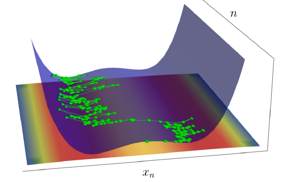
Figure 1: The stochastic difference equation given in Equation (1) describes the stochastic evolution of a process $x_{n}$ subject to a nonlinear drift $f(x)=-V^{\prime}(x)$ ($V(x)$ shown as blue shade) and a non-homogeneous diffusion $g(x)$ (rainbow coloured ground). The process is driven by multiplicative fractional driving noise $g(x)\Delta\xi^{H}$. We propose an algorithm which infers both $f(x),g(x)$ from a single finite trajectory (green dots).

2 Fractional processes

We discuss a stochastic model for nonlinear time series described by an Itô-type stochastic difference equation driven by fractional noise

$$x_{n+1}=x_{n}+f(x_{n})\Delta t+g(x_{n})\Delta\xi^{H}_{n+1}\ ,$$ (1)

where $f(x),g(x)$ denote space-dependent drift and diffusion terms of dimension $[f]=[x]/[\mathrm{time}],[g]=[x]/[\mathrm{time}]^{H}$. The process is illustrated in Figure 1. Equation (1) is the first-order discretisation (Euler-Maruyama scheme) of a stochastic differential equation driven by fractional noise [40]. While $\Delta t$ denotes the time step of the discretisation, $\Delta\xi^{H}_{n}$ is a discretised fractional Gaussian noise (fGN) [41, 42], defined by its correlation matrix

$$C_{mn}=\left\langle\Delta\xi^{H}_{m}\Delta\xi^{H}_{n}\right\rangle=(\Delta t)^{2H}\left(\left|n-m+1\right|^{2H}+\left|n-m-1\right|^{2H}-2\left|n-m\right|^{2H}\right)\ .$$ (2)

Choosing $H=\frac{1}{2}$, the noise $\Delta\xi^{H}_{n}$ is discrete standard Gaussian white noise. For $H>\frac{1}{2}$ ($H<\frac{1}{2}$), the increments $\Delta\xi^{H}_{n}$ are positively (negatively) correlated.

3 Inference method

We propose an algorithm that given a single measured trajectory $\vec{x}=\left\{x_{0},x_{1},\ldots,x_{N}\right\}$ sampled at $\Delta t$ infers the functional parameters $f(x),g(x)$ as introduced in Equation (1). We argue that $f(x)$ and $g(x)$ only introduce short-range correlations, which exponentially decay for a stationary process. We therefore expect that the asymptotic scaling of the correlation function of Equation (1) is solely determined by $H$ and $\Delta t$ and does not depend on $f(x),g(x)$. We assume that the Hurst parameter has already been estimated previously using established methods (e.g., [43, 44, 45, 46]).

The central idea is to find the functions $f$ and $g$ which maximise the log-likelihood $\ln P[\vec{x}|f,g]$ of the observed trajectory $\vec{x}$. The likelihood is obtained by measuring the likelihood of the noise realisation $\vec{\Delta\xi^{H}}=\{\Delta\xi^{H}_{1},...,\Delta\xi^{H}_{N}\}$, which together with $f$ and $g$ produces the measurement $\vec{x}$. This realisation is found by inversion of Equation (1),

$$\left(\vec{\Delta\xi^{H}}\left(\vec{x}\right)\right)_{n}=\frac{x_{n}-x_{n-1}-f(x_{n-1})\Delta t}{g(x_{n-1})}\ .$$ (3)

The probability to observe a measurement $\vec{x}$ then follows from $P_{\xi}[\vec{\Delta\xi^{H}}]$, the probability distribution of a noise realisation, by a standard change of variables in $\mathbb{R}^{N}$,

$$P[\vec{x}|f,g]=P_{\xi}\left[\vec{\Delta\xi^{H}}\left(\vec{x}\right)\right]\left|\frac{\partial\vec{\Delta\xi^{H}}}{\partial\vec{x}}\right|,$$ (4)

where the nonlinear transform (Equation 3) induces a Jacobian determinant accounting for the measure change from $\prod_{n}{\rm d}{\Delta\xi^{H}_{n}}\,$ to $\prod_{n}{\rm d}{x_{n}}\,$ [47].

Since $\vec{\Delta\xi^{H}}$ is discrete fractional Gaussian noise, its probability distribution is a $N$-dimensional Gaussian distribution. We write the distribution field-theoretically as

$$P_{\xi}=\left(\left(2\pi\right)^{N}\det[C]\right)^{-\frac{1}{2}}\exp\left(-\mathcal{A}[\Delta\xi^{H}]\right)$$ (5)

where $\mathcal{A}$ is the free action

$$\mathcal{A}[\Delta\xi^{H}]=\frac{1}{2}\left(\vec{\Delta\xi^{H}}\right)^{T}C^{-1}\vec{\Delta\xi^{H}}\ ,$$ (6)

and $C^{-1}$ is the matrix inverse of the correlation matrix given in Equation (2) [48]. Here, the non-diagonal correlation matrix accounts exactly for the full memory of the process.

The determinant $\left|\partial\vec{\Delta\xi^{H}}/\partial\vec{x}\right|$ itself is readily evaluated as ${\partial\Delta\xi^{H}_{n}}/{\partial x_{m}}$ is a lower triangular matrix with all entries vanishing for $m>n$ (see Equation (3)). Hence, the determinant is given by the product over the diagonal entries,

$${\partial\Delta\xi^{H}_{n}}/{\partial x_{n}}=g(x_{n-1})^{-1}\,.$$ (7)

This results in a log-likelihood of the measurement

$$\ln P[\vec{x}|f,g]=-\frac{1}{2}\sum_{m,n=1}^{N}\frac{x_{m}-x_{m-1}-f(x_{m-1})\Delta t}{g(x_{m-1})}C^{-1}_{m,n}\frac{x_{n}-x_{n-1}-f(x_{n-1})\Delta t}{g(x_{n-1})}-\sum_{n=0}^{N-1}\ln\left|g(x_{n})\right|,\quad$$ (8)

where we drop added normalisation constants independent of $f$ or $g$.

In the field-theoretic literature, expressions of the form of Equation (8) are well known for diagonal correlation matrices $C$, corresponding to uncorrelated noise with $H=\frac{1}{2}$, where they are referred to as Onsager-Machlup actions [36, 37, 38, 39]. These have been extensively studied to characterise the “most likely path” of a specifically parametrised stochastic process [49, 37, 50, 51, 52, 53]. In this article, we take the opposite direction and use Onsager-Machlup theory to determine which parameters render the observed path the likeliest. This means that we henceforth interpret the term in Equation (8) as a path action $\mathcal{S}[f,g|\vec{x}]=-\ln P[\vec{x}|f,g]$ in the parameters $f$ and $g$, while the path $x$ now in turn serves as a parametrisation. In doing so, we draw a connection from established (Markovian) maximum likelihood estimators [54, 28, 32] to the Onsager-Machlup formalism. We generalise these results to fractionally driven processes and hence refer to the estimation method based on maximising Equation (8) as fractional Onsager-Machlup optimisation (fOMo).

In order to estimate the optimal parameters $f$ and $g$ that maximise the likelihood of an observation $\vec{x}$, one needs to find the minimum of the path action $\mathcal{S}[f,g|\vec{x}]=-\ln P[\vec{x}|f,g]$ for some fixed observed $\vec{x}$. In order to do so, some finite-dimensional parametrisation of $f$ and $g$ is required; by introducing a set of suitable basis functions $\chi_{p}(x),\chi^{\prime}_{p^{\prime}}(x)$, one may rewrite $f(x)=\sum_{p=1}^{P}f_{p}\chi_{p}(x),g(x)=\sum_{p^{\prime}=1}^{P^{\prime}}g_{p}\chi_{p^{\prime}}(x)$ for some finite $P,P^{\prime}$ (chosen to be much smaller than $N$). The optimisation then takes place in the finite coefficients $f_{p},g_{p^{\prime}}$ of the parametrisation. Suitable basis functions include polynomials or indicator functions of disjoint intervals.

In finding the minima of the parametrised path action

$$\mathcal{S}[\{f_{p}\},\{g_{p^{\prime}}\}]=\mathcal{S}\left[\sum_{p=1}^{P}f_{p}\chi(p),\sum_{p^{\prime}=1}^{P^{\prime}}g_{p}\chi_{p^{\prime}}(x)\right]$$ (9)

in $\{f_{p}\},\{g_{p^{\prime}}\}$, it remains to discuss the uniqueness of any solution. As a derivation provided in A shows, the action has a unique global minimum in either the parameters of drift, $\{f_{p}\}$, or diffusion, $\{g_{p}\}$, when keeping the respective other set of parameters constant. When, however, considering the path action with fully free parameters $\{f_{p}\},\{g_{p^{\prime}}\}$, the picture is different. On the one hand, the action is smooth, globally bounded from below and remains partially convex along both $f_{p},g_{p}$ since both $\partial^{2}\mathcal{S}/(\partial_{f_{p}}\partial_{f_{q}})>0,\partial^{2}\mathcal{S}/(\partial_{g_{p}}\partial_{g_{q}})>0$ (see A), therefore is assured to have a minimum, and excludes the possibility of more than one isolated local minimum. On the other hand, the set of points where $\mathcal{S}$ assumes its minimum could hypothetically be a submanifold, and the optimal choice of $f,g$ could be non-unique. This degeneracy, however, is rooted in a physical ambiguity: for a specific observed time series $\vec{x}$, it is mathematically possible to modify both drift and diffusion simultaneously in a way that leaves the path probability of $\vec{x}$ unchanged. Consequently, the set of possible $\{f_{p},g_{p^{\prime}}\}$ which are equally compatible with an observation $\vec{x}$ may not be unique.

The problem of finding the optimum of Equation (8) in $f$ and $g$ is generally solved numerically. Nonetheless, in certain cases the optimum of $\mathcal{S}$ can be found analytically. These special cases are discussed in the following section.

4 Exact results

The estimation method corresponds to finding the configuration $f(x),g(x)$ that minimises $-\ln P[\vec{x}|f,g]$. Interpreting $\mathcal{S}[f,g|\vec{x}]=-\ln P[\vec{x}|f,g]$ as a field theoretic action in $f(x),g(x)$ that is parametrised by the inherently stochastic measurement $\vec{x}$ and therefore random (“disordered”), fOMo amounts to finding the minimum of $\mathcal{S}$, where simultaneously $\delta\mathcal{S}/\delta f\equiv\delta\mathcal{S}/\delta g\equiv 0$.

If $g$ is fixed, but not necessarily constant, the minimum in $f$ can be found analytically. We introduce the empirical propagator

$$[G(g)]_{m,n}=\frac{C^{-1}_{m,n}}{g(x_{m-1})g(x_{n-1})}\ ,$$ (10)

as well as the empirical velocity $v_{n}=(x_{n}-x_{n-1})/\Delta t$. Inserting these into Equation (8), the action then reads

$$\!\!\mathcal{S}=\frac{(\Delta t)^{2}}{2}\!\sum_{m,n=1}^{N}\!\left(f(x_{m-1})-v_{m}\right)G_{m,n}(g)\left(f(x_{n-1})-v_{n}\right),$$ (11)

omitting $f$-independent terms. This bilinear action corresponds to a Gaussian field theory [48] in $f(x)$ of mean $\left\langle f(x_{n-1})\right\rangle=v(x_{n})$ with non-local correlated fluctuations following $\left\langle f(x_{m-1})f(x_{n-1})\right\rangle-v_{m}v_{n}=(G^{-1})_{m,n}$.

Parametrising $f$ polynomially, $f(x)=\sum_{\ell=0}^{L-1}f_{\ell}x^{\ell}$ for some $L<N$, the optimal coefficients $\hat{f}_{\ell}$ can be found by inserting the polynomial ansatz into Equation (11) and setting $\partial\mathcal{S}/\partial\hat{f}_{\ell}=0$. The resulting action in the $f_{\ell}$ resembles the Hamiltonian of $L$ fully coupled harmonic oscillators in a confining harmonic potential which allows for a single optimal configuration corresponding to the estimate $\hat{f}_{\ell}$; a calculation provided in B shows that this minimum is given by $\hat{f}_{\ell}=(H^{-1}\vec{j})_{\ell}$, where we introduced

$$H_{\ell,k}=\sum_{m,n}x_{m-1}^{\ell}G_{m,n}x_{n-1}^{k}\qquad\mathrm{and}\qquad j_{\ell}=\sum_{m,n}G_{m,n}v_{n}x_{m-1}^{\ell}\ .$$ (12)

This estimate is exact for arbitrary inhomogeneous fixed diffusion $g(x)$; it further simplifies when $f$ is linear and $g$ constant (discretised fractional Ornstein-Uhlenbeck process, see C).

Analogously, we consider the case of $f(x)$ general but fixed. Introducing the empirical noise correlation

$$[D(f)]_{m,n}=\left(f(x_{m-1})-v_{m}\right)C_{m,n}^{-1}\left(f(x_{n-1})-v_{n}\right)$$ (13)

together with the inverse field $\psi_{n}=(g(x_{n-1}))^{-1}$, $\mathcal{S}$ reads

$$\mathcal{S}=\frac{(\Delta t)^{2}}{2}\sum_{m,n=1}^{N}\psi_{m}D_{m,n}(f)\psi_{n}-\sum_{n=1}^{N}\ln\left|\psi_{n}\right|.$$ (14)

The action resembles a fully interacting $N$-body Hamiltonian on the positive half line; the “particles” at position $\psi_{n}$ are quadratically coupled to one another, confined harmonically for $\psi_{n}\to\infty$, since $D_{nn}>0$, yet repelled from the origin by a logarithmically diverging potential giving rise to a stable minimum satisfying a self-consistency relation

$$(\Delta t)^{2}\hat{\psi}_{n}\sum_{m}D_{m,n}\hat{\psi}_{m}=1$$ (15)

for all $n$. If $g\equiv g_{0}$ is assumed to be constant (additive noise), this immediately returns $\hat{g}^{2}_{0}=(\Delta t)^{2}\sum_{m,n}D_{m,n}$. If further $H=\frac{1}{2}$, $D_{m,n}$ is diagonal, and Equation (14) resembles the Hamiltonian of $N$ non-interacting particles in a logarithmic-harmonic potential [55]. The estimate for $g_{0}$ then recovers the well-known Markovian result [54]

$$\hat{g}^{2}_{0}=\sum_{n}\left(f(x_{n-1})\Delta t-(x_{n}-x_{n-1})\right)^{2}\,.$$ (16)

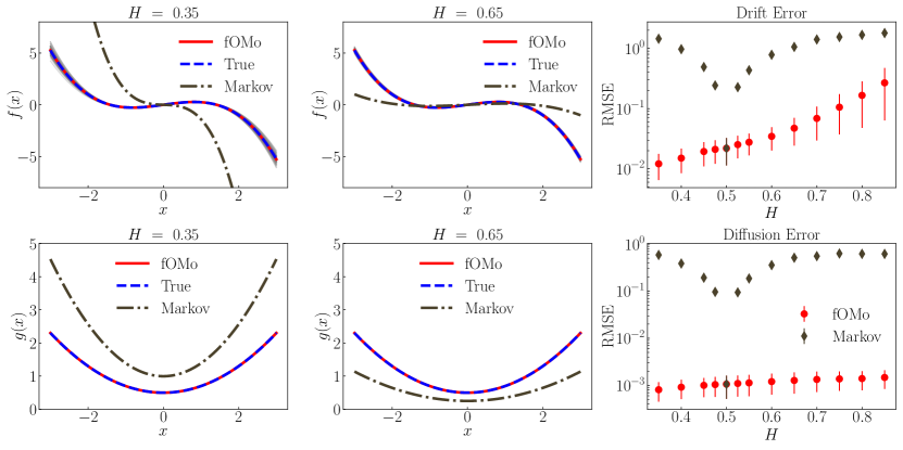
Figure 2: Inference via fOMo correctly recovers drift and diffusion in contrast to Markovian estimation. Ensemble study with $100$ trajectories with $N=10^{6},\Delta t=10^{-2}$, random initial conditions and equilibration time $T_{\mathrm{eq}}=10^{4}$ [56]. (top left and top center panels) Drift and (bottom left and bottom center panels) diffusion estimation via fOMo (red) and Markov least-squares fit (brown) for anti-correlated ($H=0.35$) and long-range correlated ($H=0.65$) dynamics. Inferred drift and diffusion of all ensemble members are plotted in light grey, only visible in (top left panel). (top right panel) Reconstruction error of drift $f(x)$ for fOMo (red) and Markovian estimate (brown). (bottom right panel) Reconstruction error of diffusion $g(x)$. Root-mean-square-errors are computed using the empirical invariant density (see text).

5 Superposition of noise processes

The method is readily adapted to processes subject to different additional Gaussian noise sources which could model, for instance, the additional coupling of the process to a heat bath. We consider a generalisation of $x_{n}$, the fractional process introduced in Equation (1), by setting

$${x_{n+1}=x_{n}+f(x_{n})\Delta t+g(x_{n})\Delta\xi^{H}_{n+1}+\eta_{n+1}}\ ,$$ (17)

where $\eta_{n}$ is an additional independent Gaussian noise term of correlation $K_{m,n}=\overline{\eta_{m}\eta_{n}}$. Repeating the previous steps in constructing the fractional Onsager-Machlup action, one inverts the new stochastic equation for $x_{n}$ to find

$$\left[\vec{\Delta\xi^{H}}(\vec{x})\right]_{n}=(x_{n}-x_{n-1}-f(x_{n-1})\Delta t-\eta_{n})/g(x_{n})\ ,$$ (18)

which one inserts into the free action $\mathcal{A}[\vec{\Delta\xi^{H}}]$ (see Equations (3, 8)). This transformation leaves the Jacobian, $\sum_{n}\left|\left(g(x_{n})\right)\right|^{-1}$, unchanged. Instead the path likelihood of $\vec{x}$ conditioned on a particular $\vec{\eta}$, Equation (8), acquires some extra terms of the form $\sum_{n}\eta_{n}a_{n}-\frac{1}{2}\sum_{m,n}\eta_{m}G_{m,n}\eta_{n}$, where we abbreviate $a_{n}=\sum_{m}G_{m,n}\left(f(x_{m-1})-v_{m}\right)\Delta t$. It remains to average over the additional noise distribution

$$P_{\eta}[\vec{\eta}]=\left((2\pi)^{N}\det K\right)^{-\frac{1}{2}}\exp\left(-1/2\sum_{m,n}\eta_{m}(K^{-1})_{mn}\eta_{n}\right)\ .$$ (19)

Carrying out the Gaussian integral in $\prod_{n}{\rm d}{\eta_{n}}\,$, one finds that the modified action is

$$\widetilde{\mathcal{S}} =-\ln\overline{P\left[\vec{x}|f,g\right]}=-\ln\int D[\vec{\eta}]P[\vec{x}|f,g,\vec{\eta}]P_{\eta}[\vec{\eta}]$$ (20)

$$=\frac{(\Delta t)^{2}}{2}\sum_{m,n=1}^{N}\left(f(x_{m-1})-v_{m}\right)\widetilde{G}_{m,n}\left(f(x_{m-1})-v_{m}\right)+\sum_{n=0}^{N-1}\ln\left|g_{n}\right|,$$ (21)

where we omit terms independent of $f,g$, and, in contrast to Equation (8), replace the empirical propagator by ${\widetilde{G}=[G^{-1}+K]^{-1}}$.

6 Fast Inversion

In order to numerically evaluate the log-likelihood given by Equation (8) the correlation matrix $C$ has to be inverted. This is an operation of computational complexity $\mathcal{O}(N^{3})$ and memory requirements of order $\mathcal{O}(N^{2})$, rendering it prohibitively costly for times series of only intermediate length ($N\sim 10^{4}$). We circumvent this problem by exploiting the Toeplitz structure of the correlation matrix; since the process is stationary, $C_{mn}$ depends on $|m-n|$ only and can be inverted efficiently [57]. In doing so, we reduce computational complexity to $\mathcal{O}(N^{2})$ and memory requirements to $\mathcal{O}(N)$ (see D for further details), rendering fOMo computationally tractable even for long time series ($N\sim 10^{6}$). This fast inversion method may be generalised to other stationary driving processes such as, for instance, tempered fractional noise [58, 59, 60].

7 Synthetic Data

We have successfully tested fOMo with various nonlinear models and illustrate a representative example in the following. We consider a model system defined by Equation (1) choosing ${f(x)=-0.25x^{3}+0.5x}$, corresponding to a double well potential, and inhomogeneous diffusion ${g(x)=0.2x^{2}+0.5}$, implying large stochastic fluctuations far away from the origin. We assume the Hurst exponent to be already determined and infer $f$ and $g$ employing fOMo (Equation (8)). In order to highlight the significance of the noise correlations, we compare this estimate to a fOMo estimate where we wrongly fix $H=\frac{1}{2}$, whence $C^{-1}$ is diagonal, effectively producing a Markovian maximum likelihood estimate (see [54]). We use polynomial basis functions for drift ($L=3$) and diffusion ($L=2$). For an ensemble of $100$ trajectories (see Figure 2 for details), we simultaneously infer drift and diffusion terms and measure the root-mean-square error (RMSE) of the inferred terms $\hat{f},\hat{g}$. Inference errors are weighted with the empirical invariant measure of the process

$$\mathrm{RMSE}(\hat{f})=\left[\sum_{n=1}^{N}\left(\hat{f}(x_{n})-f(x_{n})\right)^{2}/N\right]^{\frac{1}{2}},$$ (22)

and analogous for $g$.

Remarkably, the Markovian model underestimates (overestimates) both drift and diffusion terms for $H>\frac{1}{2}$ ($H<\frac{1}{2}$) while fOMo correctly recovers the true input functions (Figure 2) with excellent accuracy. The (anti-)correlations of the noise process lead to a wider (narrower) width of the invariant density of the process, also explaining the visible deviations of the fOMo samples from the ensemble mean for $H=0.35$ (Figure 2 (top left panel)). Markovian modelling fails to recover the double well shape of the corresponding potential in our example for $H=0.35$. The inference error of Markovian modelling steeply increases for small deviations from $H=\frac{1}{2}$, highlighting the necessity of taking fractional correlations into account.

We investigate the finite-size error scaling as a function of the trajectory length $N$ and find a drift error scaling $\mathrm{RMSE}\sim 1/\sqrt{N}$ for $H=\frac{1}{2}$, and $\mathrm{RMSE}\sim N^{\alpha}$ with $\alpha\sim H^{2}$ for $H\neq\frac{1}{2}$, while the diffusion error scaling does not show a clear trend (see E).

8 Temperature Data

We apply fOMo to daily mean temperature data recorded at Potsdam Telegrafenberg weather station, Germany. This time series consists of 130 years of uninterrupted temperature measurements downloaded from the ECAD project [61, 62]. Removing the seasonal cycle using a Fourier series, we obtain the temperature anomalies $T$, an approximately stationary time series. Temperature anomalies are long-range correlated [3, 4], monofractal [63] and have been described by overdamped models driven by fractional Gaussian noise [64, 65, 66]. We determine the Hurst exponent using detrended fluctuation analysis with a cubic polynomial (DFA3) [43, 44] and construct the correlation matrix using the estimated Hurst exponent $H\approx 0.65$ [64], and a sampling time $\Delta t=1\,\mathrm{d}$.

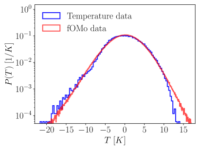
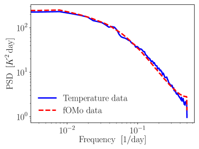
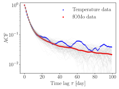
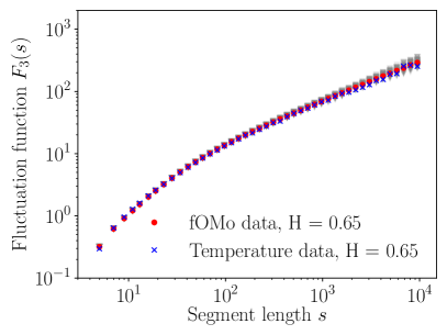
Figure 3: Stochastic fractional nonlinear model inferred with fOMo for Potsdam daily mean temperature anomalies compared to original data. Semi-transparent grey lines indicate statistics of $100$ model data trajectories, red lines are ensemble averages of model data (labelled fOMo data) and blue lines show statistics of original data. Top left: Histogram of marginal distribution. Top right: Power spectral density (PSD). Bottom left: Autocorrelation function (ACF). Bottom right: DFA3 fluctuation function.

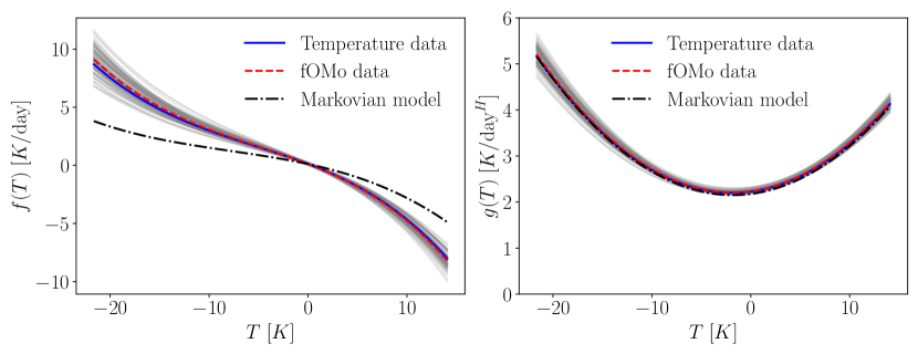
Figure 4: Drift and diffusion term estimates for Potsdam daily mean temperature anomalies. Blue lines indicate fOMo estimates from the original data and dark olive lines the Markovian estimate from original data. Semi-transparent lines show $100$ fOMo estimates from model data generated using Equation (1) and inferred drift and diffusion (blue lines). Red lines indicate the ensemble mean of the grey semi-transparent lines. Red and blue lines show excellent agreement, indicating that the estimator is free from bias.

In this model, $f$ may be interpreted as an atmospheric response function bearing the unit $[f]=K/\mathrm{day}$ and its stochastic fluctuations $g$, measured in $[g]=K/\mathrm{day}^{H}$ [65]. We use cubic and quadratic polynomial ansatzes for drift and diffusion, respectively and employ fOMo and a Markovian maximum likelihood estimate ($H=\frac{1}{2}$, see above). Since $f$ and $g$ of real-world data are not a priori known, we cannot conduct an error analysis as described above for synthetic data. However, we can compare model data with the original data and check the consistency of the model. To this end, we generate an ensemble of model time series using Equation (1) and the parameters of $f$ and $g$ obtained via fOMo. Subsequently, we compare statistics of the original data and the model data ensemble. Additionally, we infer drift and diffusion parameters from the synthetic model data ensemble and compare these with drift and diffusion obtained for the original data. For a method without bias, the mean of the inferred drift and diffusion terms should coincide with the drift and diffusion estimates of the original data. The spread of the ensemble of inferred drift and diffusion terms then gives an estimate of the errors of the inferred drift and diffusion terms due to finite samples and thus hints at the reliability of the estimate. Temperature data and synthetic model data are in very good agreement, as Figure 3 shows. Furthermore, the model is consistent since the mean of inferred drift and diffusion from model data coincides with drift and diffusion estimates from the original data (see Figure 4). The Markovian model significantly underestimates the deterministic force term compared to the force term inferred by fOMo which takes the long-range correlations into account. Unlike for the double well potential, the Markovian diffusion estimate agrees well with the fOMo estimate. This is due to the approximate linearity of $f$. In this article, we neglect the estimation error of the Hurst exponent. However, we propose the following procedure using a recently published operational method for identifying scaling regimes in attractor dimension estimation [67] which may also be employed to obtain error bars for Hurst exponents estimated via DFA [68]. At first, one determines the Hurst exponent values at the lower and upper error bars and subsequently conducts fOMo with these values. The obtained parameters for drift and diffusion terms then serve as an error estimate.

9 Conclusion

By way of a fractional generalisation of the Onsager-Machlup formalism, we create an estimation method that is able to infer functional parameters of a fully nonlinear model driven by multiplicative fractional noise from a single trajectory. Applying the algorithm to both synthetic and real data, we recover excellent estimates even for Hurst values deep in the non-Markovian regime, where ignoring the (anti-)correlations of the fluctuations leads to gross systematic errors. The method provides a needed tool for modelling real-world complex systems whose fractal nature cannot be neglected, and illuminates intriguing connections bridging time series analysis with the statistical physics of fractionally correlated many-body systems.

Appendix A Convexity in either drift or diffusion parameters

In this section, we provide more details regarding the uniqueness of the optimal solution of Equation (8), showing that the optimisation of $\mathcal{S}$ in either $f$ or $g$ is unique. Since $\mathcal{S}$ is not convex in $g$, we apply a trick and show that $\mathcal{S}$ is instead convex in $f$ and

$$\psi(x)=\frac{1}{g(x)}.$$ (23)

As

$$\frac{\delta S}{\delta g}=\underbrace{\frac{\delta\psi}{\delta g}}_{\neq 0}\frac{\delta S}{\delta\psi}$$ (24)

shows, it is then sufficient to study the optima in $\psi$, and as we assume throughout the work that $g(x)>0$, this unique solution in $\psi$ defines a unique solution for $g$ too.

The action to be considered now reads

$$\mathcal{S}[f,\psi]=\frac{\Delta t^{2}}{2}\sum_{m,n}\psi(x_{m-1})(v_{m}-f(x_{m-1}))C^{-1}_{m,n}(v_{n}-f(x_{n-1}))\psi(x_{n-1})-\sum_{n}\ln|\psi(x_{n-1})|.\quad$$ (25)

We begin by allowing for a general parametrisation of $f(x)$ and $\psi(x)$ by choosing a general set of basis functions $\chi_{p}(x)$ for $p=1,...,P$, $q=1,...,Q$ to write

$$f(x)=\sum_{p=1}^{P}f_{p}\chi_{p}(x)\qquad\psi(x)=\sum_{q=1}^{Q}\psi_{q}\chi_{q}(x).$$ (26)

Suitable choices for these basis functions include polynomials $(\chi_{p}(x)=x^{p})$ or indicator functions of disjoint intervals. The only requirement is that the decomposition in Equation (26) be unique in the coefficients $\{f_{p}\},\{\psi_{q}\}$. The optimisation of the log-likelihood (Equation (8)) then takes place in these coefficients,

$$\mathcal{S}[\{f_{p}\},\{\psi_{q}\}]=$$ (27)

$$\frac{\Delta t^{2}}{2}\sum_{m,n=1}^{N}\left(\sum_{q}\psi_{q}\chi_{q}(x_{m-1})\right)\left(v_{m}-\sum_{p}f_{p}\chi_{p}(x_{m-1})\right)C^{-1}_{m,n}\left(v_{n}-\sum_{p^{\prime}}f_{p^{\prime}}\chi_{p^{\prime}}(x_{n-1})\right)\left(\sum_{q^{\prime}}\psi_{q^{\prime}}\chi_{q^{\prime}}(x_{n-1})\right)$$

$$-\sum_{n=0}^{N-1}\ln\left|\sum_{q}\psi_{q}\chi_{q}(x_{n})\right|,$$ (28)

and therefore is a finite-dimensional optimisation problem.

It remains to show that $\mathcal{S}$ is convex in either $\{f_{p}\}$, or $\{\psi_{q}\}$. We treat $\mathcal{S}$ as a sum of a bilinear and a logarithmic part, defining $\mathcal{S}_{\rm log}=-\sum_{n=0}^{N-1}\ln\left|\sum_{q}\psi_{q}\chi_{q}(x_{n})\right|$.

It follows that the Hessian of $\mathcal{S}_{\rm log}$ is

$$[\partial^{2}\mathcal{S}_{\rm log}]_{p,q}=\frac{\partial^{2}}{\partial\psi_{p}\psi_{q}}\left(-\sum_{n=0}^{N-1}\ln\left|\sum_{p^{\prime}}\psi_{p^{\prime}}\chi_{p^{\prime}}(x_{n})\right|\right)=\sum_{n}\frac{\chi_{p}(x_{n})\chi_{q}(x_{n})}{\left(\sum_{p^{\prime}}\psi_{p^{\prime}}\chi_{p^{\prime}}(x_{n})\right)^{2}}.\quad$$ (29)

For an arbitrary vector $w_{1},...,w_{q}$, one therefore finds

$$\sum_{p,q}w_{p}[\partial^{2}\mathcal{S}_{\rm log}]_{p,q}w_{q}=\sum_{n}\frac{\left(\sum_{p}\chi_{p}(x_{n})w_{p}\right)^{2}}{\left(\sum_{p^{\prime}}\psi_{p^{\prime}}\chi_{p^{\prime}}(x_{n})\right)^{2}}>0,$$ (30)

and hence the Hessian is positive definite and $\mathcal{S}_{\rm\log}$ is convex.

We next consider the bilinar contribution to $\mathcal{S}$ and study the $P\times P$ (or $Q\times Q$)-dimensional diagonal sub-blocks of the Hessian matrix of $\mathcal{S}_{\rm bil}$ in either $\{f_{p}\}$ or $\{\psi_{q}\}$. We obtain

$$\frac{\partial\mathcal{S}}{\partial f_{p}\partial f_{q}}=\Delta t^{2}\sum_{m,n}\chi_{p}(x_{m-1})\left(\sum_{p^{\prime}}\psi_{p^{\prime}}\chi_{p^{\prime}}(x_{m-1})\right)C^{-1}_{m,n}\left(\sum_{q^{\prime}}\psi_{q^{\prime}}\chi{{}_{q}^{\prime}}(x_{n-1})\right)\chi_{q}(x_{n-1}),$$ (31)

$$\frac{\partial\mathcal{S}}{\partial\psi_{p}\partial\psi_{q}}=\Delta t^{2}\sum_{m,n}\chi_{p}(x_{m-1})\left[\left(v_{m}-\sum_{p}f_{p}\chi_{p}(x_{m-1})\right)C^{-1}_{m,n}\left(v_{n}-\sum_{q}f_{q}\chi_{q}(x_{n-1})\right)\right]\chi_{q}(x_{n-1}).\qquad\quad$$ (32)

We now consider an arbitrary vector $w_{k}$ with $k=1,...,P$ for drift and $k=1,...,Q$ for diffusion and evaluate

$$\sum_{p,q=1}^{P}w_{p}\frac{\partial\mathcal{S}}{\partial f_{p}\partial f_{q}}w_{q}\quad\mathrm{and}\quad\sum_{p,q=1}^{Q}w_{p}\frac{\partial\mathcal{S}}{\partial\psi_{p}\partial\psi_{q}}w_{q}\,.$$ (33)

The first term corresponds to

$$\sum_{p,q=1}^{P}w_{p}\frac{\partial\mathcal{S}}{\partial f_{p}\partial f_{q}}w_{q}=$$ (34)

$$\Delta t^{2}\sum_{m,n}\left(\sum_{p}w_{p}\chi_{p}(x_{m-1})\right)\left(\sum_{p^{\prime}}\psi_{p^{\prime}}\chi_{p^{\prime}}(x_{m-1})\right)C^{-1}_{m,n}\left(\sum_{q^{\prime}}\psi_{q^{\prime}}\chi{{}_{q}^{\prime}}(x_{n-1})\right)\left(\sum_{q}w_{q}\chi_{q}(x_{n-1})\right).\qquad\quad$$ (35)

Introducing

$$W^{-}_{n} =\sum_{p}w_{p}\chi_{p}(x_{n-1})$$ (36)

$$\Psi_{n} =\sum_{q^{\prime}}\psi_{q^{\prime}}\chi{{}_{q}^{\prime}}(x_{n-1})=\psi(x_{n-1}),$$ (37)

this reads

$$\sum_{p,q=1}^{P}w_{p}\frac{\partial\mathcal{S}}{\partial f_{p}\partial f_{q}}w_{q}=\frac{\Delta t^{2}}{2}\sum_{m,n}W_{m}^{-}\Psi_{m}C^{-1}_{m,n}\Psi_{n}W^{-}_{n}.$$ (38)

Since $C^{-1}$ is the inverse of a Gaussian correlation matrix it is a positive definite matrix, and therefore

$$\sum_{p,q=1}^{P}w_{p}\frac{\partial\mathcal{S}}{\partial f_{p}\partial f_{q}}w_{q}>0$$ (39)

for all choices of $w$. Hence $\mathcal{S}$ is convex in $f_{p}$.

To study convexity in $\psi$, we evaluate the second term which is

$$\sum_{q,q^{\prime}=1}^{Q}w_{q}\frac{\partial\mathcal{S}}{\partial\psi_{q}\partial\psi_{q^{\prime}}}w_{q^{\prime}}=$$ (40)

$$\Delta t^{2}\sum_{m,n}\left(\sum_{q}w_{q}\chi_{q}(x_{m-1})\right)\left(v_{m}-\sum_{p}f_{p}\chi_{p}(x_{m-1})\right)C^{-1}_{m,n}\left(v_{n}-\sum_{p^{\prime}}f_{p^{\prime}}\chi_{p^{\prime}}(x_{n-1})\right)\left(\sum_{q^{\prime}}w_{q^{\prime}}\chi_{q^{\prime}}(x_{n-1})\right).$$

Further introducing

$$W^{+}_{n} =\sum_{q}w_{q}\chi_{q}(x_{n-1})$$ (42)

$$V_{n} =v_{n}-\sum_{p}f_{p}\chi_{p}(x_{n-1}),$$ (43)

this reads

$$\sum_{p,q=1}^{Q}w_{p}\frac{\partial\mathcal{S}}{\partial\psi_{p}\partial\psi_{q}}w_{q}=\Delta t^{2}\sum_{m,n}W^{+}_{m}V_{m}C^{-1}_{m,n}W^{+}_{n}V_{n}.$$ (44)

Again, positive definiteness of $C^{-1}$ implies that

$$\sum_{p,q=1}^{Q}w_{p}\frac{\partial\mathcal{S}}{\partial\psi_{p}\partial\psi_{q}}w_{q}>0$$ (45)

for all choices of $w$ and hence $\mathcal{S}$ is convex in $\Psi$.

Since both Hessians in $\{f_{p}\},\{\psi_{p}\}$ of the log-likelihood are positiv definite, the log-likelihood is convex in both subspaces and possesses a global minimum in each of the subspaces.

Appendix B Optimal drift estimate for fixed diffusion

We provide further details on the analytic solution given for the minimum solution $\delta S/\delta\hat{f}\equiv 0$ when $g(x)$ is fixed, see Equation (11).

Setting out from Equations (3, 8), the full action reads

$$\mathcal{S}[f,g|\vec{x}]=\frac{1}{2}\sum_{m,n}\frac{\left(f(x_{m-1})\Delta t-(x_{m}-x_{m-1})\right)}{g(x_{m})}C^{-1}_{m,n}\frac{\left(f(x_{n-1})\Delta t-(x_{n}-x_{n-1})\right)}{g(x_{n})}\ .$$ (46)

Since we do not vary $g(x)$, we absorb the inhomogeneous diffusivity into the inverse of the fractional correlation matrix (see Equation (2)) and introduce the effective propagator

$$G_{m,n}=\frac{C^{-1}_{m,n}}{g(x_{m-1})g(x_{n-1})}.$$ (47)

Further introducing $v_{n}=(x_{n}-x_{n-1})/\Delta t$, one readily recovers the expression given in Equation (11).

Technically, this action is minimised by the “empirical force” $f(x_{n-1})=v_{n}$. In order to effectively average over the fluctuations of $x_{n}$, however, a low-dimensional representation of $f$ is more suitable. We choose a polynomial representation, i.e., $f(x)=\sum_{\ell=0}^{L-1}f_{\ell}x^{\ell}$ with $L\ll N$. Inserting this ansatz into Equation (46), one finds

$$\mathcal{S}[f,g|\vec{x}] =\frac{(\Delta t)^{2}}{2}\sum_{\ell,k}\sum_{m,n}\left(f_{\ell}x_{m-1}^{\ell}-v_{m}\right)G_{m,n}\left(f_{k}x_{n-1}^{k}-v_{n}\right)$$ (48)

$$=\frac{(\Delta t)^{2}}{2}\left\{\sum_{\ell,k}f_{\ell}f_{k}\left(\sum_{m,n}x_{m-1}^{\ell}G_{m,n}x_{n-1}^{l}\right)-2\sum_{\ell}f_{\ell}\left(\sum_{m,n}x_{m-1}^{\ell}G(g)_{m,n}(x_{n}-x_{n-1})\right)\right\}+\ldots,\qquad$$ (49)

where we ignore $f$-independent terms. Identifying

$$H_{\ell,k} =\sum_{m,n}x_{m-1}^{\ell}G(g)_{m,n}x_{n-1}^{k}$$ (50)

$$J_{\ell} =\sum_{m,n}x_{m-1}^{\ell}G(g)_{m,n}(x_{n}-x_{n-1}),$$ (51)

the optimal point $\nabla_{\hat{f}}\mathcal{S}=0$ implies $(\Delta t)^{2}\left\{H\hat{f}-J\right\}=0$, and hence $\hat{f}=H^{-1}J$ as stated in the main text.

Appendix C fOMo estimation for the fractional Ornstein-Uhlenbeck process

In the special case of linear drift and constant diffusion, Equation (1) recovers the Euler-Maruyama discretisation of a fractional Ornstein Uhlenbeck process, i.e.,

$$x_{n+1}-x_{n}=-fx_{n}\Delta t+g\Delta\xi^{H}_{n+1}.$$ (52)

Accordingly parametrising $f(x)=fx,g(x)=g$, the fractional Onsager Machlup action (Equation (8)) reduces to the two-dimensional function

$$\mathcal{S}[f,g]=\frac{(\Delta t)^{2}}{2g^{2}}\sum_{m,n}\left(f-v_{m}\right)C_{m,n}^{-1}\left(f-v_{n}\right)+\ln|g|.$$ (53)

The minimum in $f$ is $g$-independent and is given by

$$\hat{f}=\frac{\sum_{m,n}C^{-1}_{m,n}v_{n}}{\sum_{m,n}C_{m,n}^{-1}},$$ (54)

which extends [28] from white noise to processes driven by Gaussian noise with arbitrary correlations. The minimum in $g$ is given by

$$\hat{g}^{2}=(\Delta t)^{2}\sum_{m,n}\left(\hat{f}-v_{m}\right)C_{m,n}^{-1}\left(\hat{f}-v_{n}\right)\ .$$ (55)

Appendix D A Note on the Numerics

In this section, we elaborate on the computation of the stochastic action given by Equation (8). For stationary processes, the autocovariance function solely depends on the difference between two time instances. Hence, the covariance matrix $C_{ij}$ is a $(N-1)\times(N-1)$ symmetric Toeplitz matrix, where $N$ is the length of the time series, i.e. ${C_{ij}=(\Delta t)^{2H}\times\left(\left|i-j+1\right|^{2H}+\left|i-j-1\right|^{2H}-2\left|i-j\right|^{2H}\right)}=:C(|i-j|\Delta t)$, in which $i,j\in\{1,\ldots,N-1\}$. We compute the inverse correlation matrix, the propagator, exploiting this fact. The inverse of a Toeplitz matrix may be expressed as [57]

$$C^{-1}=T_{1}U_{1}+T_{2}U_{2}\,,$$ (56)

in which $T_{1}$ and $T_{2}$ are Toeplitz matrices and $U_{1}$, $U_{2}$ are upper triangular matrices with Toeplitz structure:

$$T_{1}=\left(\begin{array}[]{cccc}y_{1}&y_{n}&\ldots&y_{2}\\ y_{2}&y_{1}&\ddots&\\ \vdots&\ddots&\ddots&y_{n}\\ y_{n}&\ldots&y_{2}&y_{1}\end{array}\right)\,,\quad U_{1}=\left(\begin{array}[]{cccc}1&-x_{n}&\ldots&-x_{2}\\ &1&\ddots&\vdots\\ &&\ddots&-x_{n}\\ &&&1\end{array}\right)$$ (65)

$$T_{2}=\left(\begin{array}[]{cccc}x_{1}&x_{n}&\ldots&x_{2}\\ x_{2}&x_{1}&\ddots&\vdots\\ \vdots&\ddots&\vdots&x_{n}\\ x_{n}&\ldots&x_{2}&x_{1}\end{array}\right)\,,\quad U_{2}=\left(\begin{array}[]{cccc}0&y_{n}&\ldots&y_{2}\\ &0&\ddots&\vdots\\ &&\ddots&y_{n}\\ &&&0\end{array}\right)\,.$$ (74)

The vectors $x$ and $y$ are solutions to the linear equations

$$Cx=h\,,$$ (75)

$$Cy=e_{1}\,,$$ (76)

$$e_{1}=\left(\begin{array}[]{c}1\\ 0\\ \vdots\\ 0\end{array}\right)\,, \quad h=\left(\begin{array}[]{c}0\\ C((N-1)\Delta t)-C(\Delta t)\\ \vdots\\ C(2\Delta t)-C((N-2)\Delta t)\\ C(\Delta t)-C((N-1)\Delta t)\end{array}\right)\,.$$ (86)

The matrices $T$ and $U$ are entirely determined by $x$ and $y$. Hence, only these two vectors have to be saved during computation. We obtain $x$ and $y$ solving the linear equations Equation (75) and Equation (76) using the Levinson-Durbin algorithm, which has complexity $\mathcal{O}(N^{2})$. Thus, the action reads

$$\mathcal{S}[\vec{x}|f,g] =\frac{(\Delta t)^{2}}{2}\sum_{m,n=1}^{N}\frac{\left(f_{m-1}-v_{m}\right)}{g_{m-1}}\,(T_{1}U_{1}+T_{2}U_{2})_{mn}\,\frac{\left(f_{n-1}-v_{n}\right)}{g_{n-1}}+\sum_{n=0}^{N-1}\ln|g_{n}|\qquad$$ (87)

which are repeated Toeplitz matrix multiplications. During the optimisation of $f$ and $g$, $C^{-1}$ does not change. Thus, we only compute Toeplitz matrix multiplications throughout the optimisation.

Appendix E Finite-Size Error Scaling of Synthetic Data

We investigate the finite-size error scaling as a function of the trajectory length $N$ of synthetic data generated from the model (see main text)

$$x_{n+1}=x_{n}+\Delta t(-0.25\,x_{n}^{3}+0.5\,x_{n})+(0.2\,x_{n}^{2}+0.5)\Delta\xi_{n+1}^{H}\,,$$

with $\Delta t=0.01$. For fixed Hurst exponent and an ensemble of $100$ trajectories, we fit a power law to the asymptotic scaling of the RMSE in $N$, up to $N=2\times 10^{6}$. In accordance with the central limit theorem, we find $\mathrm{RMSE}\sim 1/\sqrt{N}$ in the case $H=\frac{1}{2}$ for both drift and diffusion. However, we observe that the inference error of the drift for $H\neq\frac{1}{2}$ scales according to $\mathrm{RMSE}\sim N^{\alpha}$ with $\alpha\sim H^{2}$, while the diffusion error scaling does not show a clear trend. We further observe qualitatively similar error scaling for other toy models, e.g. monostable potentials. Scaling behaviour deviating from the central limit theorem for correlated data is also observed for the sample mean of correlated Gaussian random variables. Its standard deviation scales like $\sigma_{\mu_{N}}\sim N^{H-1}$ [69, 70]. Hence, the convergence speed of the sample mean depends on the strengths of the correlations, also allowing faster convergence for $H<\frac{1}{2}$, which we observe as well.

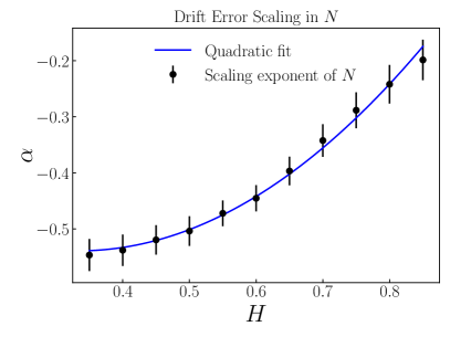
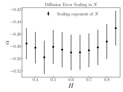
Figure 5: Toy model with double well potential and quadratic diffusion term. Error scaling in trajectory length $N$ as a function of the Hurst exponent $H$.

Appendix F Potsdam Temperature Data

In the main text, we demonstrate fOMo by reconstructing a stochastic model from daily mean temperature anomalies recorded at Potsdam Telegrafenberg weather station, Potsdam, Germany. Here, we elaborate on the procedure. We obtain the temperature anomalies by subtracting the seasonal cycle. In the main text, we state that the resulting time series is approximately stationary. In fact, there are slow-mode variations in the time series as well as a warming trend. However, these only marginally violate the stationarity of the time series. We thus abstain from subtracting an additional trend from the data besides seasonality. Furthermore, we neglect measurement errors in our analysis since they are sufficiently small compared to the dynamics.

References

- [1] Metzler R, Jeon J H, Cherstvy A G and Barkai E 2014 Phys. Chem. Chem. Phys. 16(44) 24128–24164 URL http://dx.doi.org/10.1039/C4CP03465A
- [2] Hurst H E 1951 Trans. Am. Soc. Civ. Eng. 116 770
- [3] Bunde A, Havlin S, Koscielny-Bunde E and Schellnhuber H J 2001 Physica A: Statistical Mechanics and its Applications 302 255–267 ISSN 0378-4371 URL https://www.sciencedirect.com/science/article/pii/S0378437101004691
- [4] Eichner J F, Koscielny-Bunde E, Bunde A, Havlin S and Schellnhuber H J 2003 Phys. Rev. E 68(4) 046133 URL https://link.aps.org/doi/10.1103/PhysRevE.68.046133
- [5] Bunde A, Eichner J F, Kantelhardt J W and Havlin S 2005 Phys. Rev. Lett. 94(4) 048701 URL https://link.aps.org/doi/10.1103/PhysRevLett.94.048701
- [6] Kantelhardt J W, Koscielny-Bunde E, Rybski D, Braun P, Bunde A and Havlin S 2006 J. Geophys. Res. Atmos. 111 URL https://agupubs.onlinelibrary.wiley.com/doi/abs/10.1029/2005JD005881
- [7] Voss R F 1992 Phys. Rev. Lett. 68 3805
- [8] Chatzidimitriou-Dreismann C and Larhammar D 1993 Nature 361 212–213
- [9] Höfling F and Franosch T 2013 Rep. Prog. Phys. 76 046602 ISSN 0034-4885 URL https://dx.doi.org/10.1088/0034-4885/76/4/046602
- [10] Wan K Y and Goldstein R E 2014 Phys. Rev. Lett. 113(23) 238103 URL https://link.aps.org/doi/10.1103/PhysRevLett.113.238103
- [11] Palva J M, Zhigalov A, Hirvonen J, Korhonen O, Linkenkaer-Hansen K and Palva S 2013 Proc. Natl. Acad. Sci. U.S.A. 110 3585–3590
- [12] Teka W, Marinov T M and Santamaria F 2014 PLoS Comput. Biol. 10 e1003526 ISSN 1553-7358 URL https://dx.plos.org/10.1371/journal.pcbi.1003526
- [13] Muñoz Gil G, Volpe G, Garcia-March M A, Aghion E, Argun A, Hong C B, Bland T, Bo S, Conejero J A, Firbas N, Garibo i Orts O, Gentili A, Huang Z, Jeon J H, Kabbech H, Kim Y, Kowalek P, Krapf D, Loch-Olszewska H, Lomholt M A, Masson J B, Meyer P G, Park S, Requena B, Smal I, Song T, Szwabiński J, Thapa S, Verdier H, Volpe G, Widera A, Lewenstein M, Metzler R and Manzo C 2021 Nat. Commun. 12 6253 ISSN 2041-1723 URL https://doi.org/10.1038/s41467-021-26320-w
- [14] Bzdok D, Altman N and Krzywinski M 2018 Nat. Methods 15 233–234 ISSN 1548-7105 URL https://doi.org/10.1038/nmeth.4642
- [15] Carleo G, Cirac I, Cranmer K, Daudet L, Schuld M, Tishby N, Vogt-Maranto L and Zdeborová L 2019 Rev. Mod. Phys. 91(4) 045002 URL https://doi.org/10.1103/RevModPhys.91.045002
- [16] Cichos F, Gustavsson K, Mehlig B and Volpe G 2020 Nature Machine Intelligence 2 94–103 ISSN 2522-5839 URL https://doi.org/10.1038/s42256-020-0146-9
- [17] Rao B P 2011 Statistical inference for fractional diffusion processes (Chichester, UK: John Wiley & Sons) URL https://www.wiley.com/en-gb/Statistical+Inference+for+Fractional+Diffusion+Processes-p-9780470975763
- [18] Burnecki K and Weron A 2014 J. Stat. Mech.: Theory Exp. 2014 P10036
- [19] Graves T, Gramacy R B, Franzke C L and Watkins N W 2015 Nonlinear Process Geophys 22 679–700
- [20] Kubilius K, Mishura Y and Ralchenko K 2017 Parameter Estimation in Fractional Diffusion Models (Cham, Switzerland: Springer) URL https://doi.org/10.1007/978-3-319-71030-3
- [21] Thapa S, Lomholt M A, Krog J, Cherstvy A G and Metzler R 2018 Phys. Chem. Chem. Phys. 20(46) 29018–29037 URL http://dx.doi.org/10.1039/C8CP04043E
- [22] Siegert S, Friedrich R and Peinke J 1998 Phys. Lett. A 243 275 – 280 ISSN 0375-9601 URL http://www.sciencedirect.com/science/article/pii/S0375960198002837
- [23] Ragwitz M and Kantz H 2001 Phys. Rev. Lett. 87(25) 254501 URL https://link.aps.org/doi/10.1103/PhysRevLett.87.254501
- [24] Böttcher F, Peinke J, Kleinhans D, Friedrich R, Lind P G and Haase M 2006 Phys. Rev. Lett. 97(9) 090603 URL https://link.aps.org/doi/10.1103/PhysRevLett.97.090603
- [25] Beheiry M E, Dahan M and Masson J B 2015 Nat. Methods 12 594–595 ISSN 1548-7105 URL https://doi.org/10.1038/nmeth.3441
- [26] Gouasmi A, Parish E J and Duraisamy K 2017 Proceedings of the Royal Society A: Mathematical, Physical and Engineering Sciences 473 20170385 (Preprint https://royalsocietypublishing.org/doi/pdf/10.1098/rspa.2017.0385) URL https://royalsocietypublishing.org/doi/abs/10.1098/rspa.2017.0385
- [27] Lehle B and Peinke J 2018 Phys. Rev. E 97(1) 012113 URL https://link.aps.org/doi/10.1103/PhysRevE.97.012113
- [28] Pérez García L, Donlucas Pérez J, Volpe G, V Arzola A and Volpe G 2018 Nat. Commun. 9 5166 ISSN 2041-1723 URL https://doi.org/10.1038/s41467-018-07437-x
- [29] Tabar R 2019 Analysis and data-based reconstruction of complex nonlinear dynamical systems vol 730 (Cham, Switzerland: Springer) URL https://link.springer.com/book/10.1007/978-3-030-18472-8
- [30] Brückner D B, Ronceray P and Broedersz C P 2020 Phys. Rev. Lett. 125(5) 058103 URL https://link.aps.org/doi/10.1103/PhysRevLett.125.058103
- [31] Frishman A and Ronceray P 2020 Phys. Rev. X 10(2) 021009 URL https://link.aps.org/doi/10.1103/PhysRevX.10.021009
- [32] Ferretti F, Chardès V, Mora T, Walczak A M and Giardina I 2020 Phys. Rev. X 10(3) 031018 URL https://link.aps.org/doi/10.1103/PhysRevX.10.031018
- [33] Willers C and Kamps O 2021 Eur. Phys. J. B 94 149 ISSN 1434-6036 URL https://doi.org/10.1140/epjb/s10051-021-00149-0
- [34] Weiss M 2013 Phys. Rev. E 88 010101 URL https://link.aps.org/doi/10.1103/PhysRevE.88.010101
- [35] Saelens W, Cannoodt R, Todorov H and Saeys Y 2019 Nat Biotechnol 37 547–554 ISSN 1546-1696 URL https://www.nature.com/articles/s41587-019-0071-9
- [36] Onsager L and Machlup S 1953 Phys. Rev. 91(6) 1505–1512 URL https://link.aps.org/doi/10.1103/PhysRev.91.1505
- [37] Dürr D and Bach A 1978 Commun. Math. Phys. 60 153–170 ISSN 1432-0916 URL https://doi.org/10.1007/BF01609446
- [38] Täuber U C 2014 Critical dynamics (Cambridge, UK: Cambridge University Press)
- [39] Cugliandolo L F and Lecomte V 2017 J. Phys. A Math. Theor. 50 345001 URL https://dx.doi.org/10.1088/1751-8121/aa7dd6
- [40] Pipiras V and Taqqu M S 2017 Long-Range Dependence and Self-Similarity Cambridge Series in Statistical and Probabilistic Mathematics (Cambridge University Press)
- [41] Mandelbrot B B and Van Ness J W 1968 SIAM Rev. 10 422–437
- [42] Mandelbrot B B and Wallis J R 1969 Water Resour. Res 5 321–340
- [43] Peng C K, Buldyrev S V, Havlin S, Simons M, Stanley H E and Goldberger A L 1994 Phys. Rev. E 49(2) 1685–1689 URL https://link.aps.org/doi/10.1103/PhysRevE.49.1685
- [44] Höll M, Kiyono K and Kantz H 2019 Phys. Rev. E 99(3) 033305 URL https://link.aps.org/doi/10.1103/PhysRevE.99.033305
- [45] Abry P and Veitch D 1998 IEEE Trans. Inf. Theory 44 2–15
- [46] Bo S, Schmidt F, Eichhorn R and Volpe G 2019 Phys. Rev. E 100(1) 010102 URL https://link.aps.org/doi/10.1103/PhysRevE.100.010102
- [47] Devore J L, Berk K N and Carlton M A 2021 Modern Mathematical Statistics with Applications 3rd ed Springer Texts in Statistics (Cham, Switzerland: Springer) ISBN 9781461403906,1461403901
- [48] Zinn-Justin J 2002 Quantum Field Theory and Critical Phenomena (Oxford University Press) ISBN 978-0-19-850923-3 URL https://academic.oup.com/book/11638
- [49] Horsthemke W and Bach A 1975 Z Physik B 22 189–192
- [50] Adib A B 2008 J. Phys. Chem. B 112 5910–5916
- [51] Kappler J and Adhikari R 2020 Phys. Rev. Res. 2(2) 023407 URL https://link.aps.org/doi/10.1103/PhysRevResearch.2.023407
- [52] Gladrow J, Keyser U F, Adhikari R and Kappler J 2021 Phys. Rev. X 11(3) 031022 URL https://link.aps.org/doi/10.1103/PhysRevX.11.031022
- [53] Kieninger S and Keller B G 2021 J. Chem. Phys. 154 094102
- [54] Kleinhans D 2012 Phys. Rev. E 85(2) 026705 URL https://link.aps.org/doi/10.1103/PhysRevE.85.026705
- [55] Ryabov A, Dierl M, Chvosta P, Einax M and Maass P 2013 J. Phys. A: Math. Theor. 46 075002 ISSN 1751-8121
- [56] Davies R B and Harte D S 1987 Biometrika 74 95–101 ISSN 0006-3444 URL https://doi.org/10.1093/biomet/74.1.95
- [57] Lv X G and Huang T Z 2007 Appl. Math. Lett. 20 1189–1193 ISSN 0893-9659 URL https://www.sciencedirect.com/science/article/pii/S0893965907000535
- [58] Meerschaert M M and Sabzikar F 2013 Stat. Probab. Lett 83 2269–2275 ISSN 0167-7152
- [59] Liemert A, Sandev T and Kantz H 2017 Phys. A: Stat. Mech. Appl. 466 356–369
- [60] Molina-Garcia D, Sandev T, Safdari H, Pagnini G, Chechkin A and Metzler R 2018 New J. Phys. 20 103027 URL https://iopscience.iop.org/article/10.1088/1367-2630/aae4b2/meta
- [61] Klein Tank A M G, Wijngaard J B, Können G P, Böhm R, Demarée G, Gocheva A, Mileta M, Pashiardis S, Hejkrlik L, Kern-Hansen C, Heino R, Bessemoulin P, Müller-Westermeier G, Tzanakou M, Szalai S, Pálsdóttir T, Fitzgerald D, Rubin S, Capaldo M, Maugeri M, Leitass A, Bukantis A, Aberfeld R, van Engelen A F V, Forland E, Mietus M, Coelho F, Mares C, Razuvaev V, Nieplova E, Cegnar T, Antonio López J, Dahlström B, Moberg A, Kirchhofer W, Ceylan A, Pachaliuk O, Alexander L V and Petrovic P 2002 Int. J. Climatol. 22 1441–1453 URL https://rmets.onlinelibrary.wiley.com/doi/abs/10.1002/joc.773
- [62] Besselaar E J M V D, Tank A M G K, Schrier G V D, Abass M S, Baddour O, Engelen A F V, Freire A, Hechler P, Laksono B I, Iqbal, Jilderda R, Foamouhoue A K, Kattenberg A, Leander R, Güingla R M, Mhanda A S, Nieto J J, Sunaryo, Suwondo A, Swarinoto Y S and Verver G 2015 Bull Am Meteorol Soc 96 16–21 ISSN 00030007, 15200477 URL http://www.jstor.org/stable/26219458
- [63] Bunde A and Ludescher J 2017 Long-Term Memory in Climate: Detection, Extreme Events, and Significance of Trends (Cambridge University Press) p 318–339
- [64] Massah M and Kantz H 2016 Geophys. Res. Lett. 43 9243–9249 URL https://agupubs.onlinelibrary.wiley.com/doi/abs/10.1002/2016GL069555
- [65] Király A and Jánosi I M 2002 Phys. Rev. E 65(5) 051102 URL https://link.aps.org/doi/10.1103/PhysRevE.65.051102
- [66] Kassel J A and Kantz H 2022 Phys. Rev. Research 4(1) 013206 URL https://link.aps.org/doi/10.1103/PhysRevResearch.4.013206
- [67] Deshmukh V, Bradley E, Garland J and Meiss J D 2021 Chaos: An Interdisciplinary Journal of Nonlinear Science 31 123102 URL https://doi.org/10.1063/5.0069365
- [68] Phillips E T, Höll M, Kantz H and Zhou Y 2023 Phys. Rev. E 108(3) 034301 URL https://link.aps.org/doi/10.1103/PhysRevE.108.034301
- [69] Polotzek K 2021 Modeling and analysis of non-Gaussian long-range correlated data-Extreme value theory and effective sample sizes with applications to precipitation data Ph.D. thesis Technische Universität Dresden Dresden
- [70] Massah M, Aghion E, Kassel J A and Kantz H 2023 In preparation