Criticality-enhanced Electromagnetic Field Sensor with Single Trapped Ions

Abstract

We propose and analyze a driven-dissipative quantum sensor that is continuously monitored close to a dissipative critical point. The sensor relies on the critical open Rabi model with the spin and phonon degrees of freedom of a single trapped ion to achieve criticality-enhanced sensitivity. Effective continuous monitoring of the sensor with nearly unit efficiency is realized via a co-trapped ancilla ion that switches between dark and bright internal states conditioned on a ‘jump’ of the phonon population. We demonstrate that the critical sensor achieves a scaling beyond the standard shot noise limit under realistic conditions and is robust to experimental imperfections.

Introduction – A closed quantum many-body system is highly sensitive to even small variations in the Hamiltonian parameters near quantum critical points (CPs). This sensitivity is quantified by the divergent susceptibilities of its ground state and directly leads to a divergent quantum Fisher information (QFI), a key metric that characterizes the ultimately achievable precision of a many-body sensor. This observation has motivated numerous criticality-enhanced sensing proposals  [1, 2, 3, 4, 5, 6, 7, 8, 9, 10, 11, 12, 13], offering promising alternatives towards quantum-enhanced sensitivity beyond conventional schemes that rely on the direct preparation of entangled states [14, 15, 16].

However, typical quantum sensors are intrinsically open systems both because they need to be interrogated by measurements and because they are naturally coupled to environmental noise. Hence, a natural step for criticality-enhanced sensing is to look at open critical system undergoing dissipative phase transitions [17, 18, 19, 20, 21, 22, 23]. In analogy to the case of a closed system, at a dissipative CP the susceptibilities of the steady state of the open system exhibit universal divergent scaling behavior resulting in enhanced sensing precision. Moreover, in sharp contrast to closed systems, open critical systems continuously exchange radiation quanta with their environment, making possible the sensing of unknown parameters through continuous measurement of the emission field. This approach naturally avoids the detrimental effect of critical slowing down in steady state preparation which would need to be factored into the resource budget of the metrology scheme and may lead to a considerable reduction in the achievable precision. Ultimately, the precision of the critical open quantum sensor is characterized by the global QFI of the joint system and environment state. In a previous work [10], we have established a general scaling theory of the global QFI at dissipative CPs, by relating its scaling exponents to the critical exponents of the underlying CP. However, a direct implementation of such sensing schemes requires highly efficient detection of the emission field emanated from engineered critical open systems. This is typically accomplished through the use of high finesse optical cavities, which is, however, a challenging experimental task.

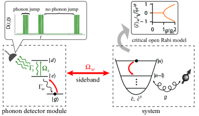
Figure 1: Schematics of the proposed criticality enhanced sensor. The sensor consists of a coupled bosonic mode and qubit system that realizes the critical open Rabi model. The emission quanta of the bosonic mode can be monitored via a phonon detector module with high efficiency. In particular, via sideband coupling to the auxiliary spin, a single boson emission $\ket{n}\to\ket{n-1}$ switches the spin from the dark state $\ket{g}$ to the bright state $\ket{e}$ measured with standard electron shelving techniques. An additional decay channel $\ket{e}\to\ket{g}$ restores the internal state of the spin, allowing for continuous phonon counting at near perfect effective efficiency.

Here we overcome this challenge with the proposal of a general cavity-free scheme for the highly efficient detection of the emission field. Our scheme is inspired by entanglement-based spectroscopy [24, 25] and is illustrated in Fig. 1 at the example of detecting the emission quanta of a bosonic mode: to detect a single emission event we correlate the phonon states with an auxiliary spin-$\frac{1}{2}$ via sideband pulses that achieve the transition $\ket{n-1}\bra{n}\otimes\ket{e}\bra{g}$ ($\ket{n}$ is the bosonic Fock state) such that the event $\ket{n}\to\ket{n-1}$ is correlated with population transfer $\ket{g}\to\ket{e}$ of the auxiliary spin. The latter can be measured via standard electron shelving techniques with nearly unit efficiency [26]. The dissipative channel $\ket{e}\to\ket{g}$ of the spin restores its internal state thus enabling continuous monitoring of the emission quanta of the bosonic mode with high efficiency, a key requirement for the implementation of criticality enhanced open sensors. As a demonstration, we apply our general scheme to the design a critical electromagnetic field sensor consisting of an open Rabi model realized with trapped ions, where the auxiliary read-out spin is realized as a co-trapped ion, and discuss its experimental performance under realistic noise and system imperfections.

Open Rabi Model – We consider a bosonic mode coupled to a qubit according to the quantum Rabi Hamiltonian (throughout this article $\hbar=1$),

$$\hat{H}_{R}=\omega\hat{c}^{\dagger}\hat{c}+\frac{\Omega}{2}\hat{\sigma}_{z}-\lambda(\hat{c}+\hat{c}^{\dagger})\hat{\sigma}_{x},$$ (1)

where $\hat{c}$ $(\hat{c}^{\dagger})$ denotes the annihilation (creation) operator of the mode, $\hat{\sigma}_{z,x}$ are the Pauli matrices of the qubit, $\omega$ is the mode’s frequency, $\Omega$ is the qubit transition frequency and $\lambda$ is the coupling strength of the qubit-mode interaction. We assume that the bosonic mode is damped by a Markovian reservoir at a dissipation rate $\kappa$, and as a result the dynamics of the open boson-qubit system can be described by a Lindblad master equation (LME) [10, 27, 5]

$$\dot{\rho}=-i[\hat{H}_{\rm R},\rho]+\kappa\left(2\hat{c}\rho\hat{c}^{\dagger}-\{\hat{c}^{\dagger}\hat{c},\rho\}\right).$$ (2)

For such a zero-dimensional model, we can introduce the frequency ratio $\eta=\Omega/\omega$ as the effective system size, with $\eta\to\infty$ corresponding to the thermodynamic limit [27]. In the limit $\eta\rightarrow\infty$, when the dimensionless coupling strength $g=2\lambda/\sqrt{\omega\Omega}$ is tuned across the critical point (CP) $g_{c}=\sqrt{1+(\kappa/\omega)^{2}}$, the steady state of Eq. (2) breaks spontaneously the ${\mathbb{Z}}_{2}$ parity symmetry ($\hat{c}\to-\hat{c},\hat{\sigma}_{x}\to-\hat{\sigma}_{x}$) of the model, therefore undergoing a continuous dissipative phase transition [27]: from a normal phase for $g<g_{c}$, as characterized by the order parameter $\langle\hat{c}\rangle_{\rm st}=0$, with $\langle\cdot\rangle_{\rm st}\equiv{\rm tr}[\rho_{\rm st}(\cdot)]$; to a superradiant phase for $g>g_{c}$, where $\langle\hat{c}\rangle_{\rm st}\neq 0$.

The CP is characterized by a few critical exponents which have been extracted via numerical finite-size scaling [10, 27], in particular $z=1$ is the dynamic and $\nu=2$ is the correlation length critical exponent. Moreover, at the CP the mean excitation of the bosonic mode, $\hat{n}:=\hat{c}^{\dagger}\hat{c}$, diverges as $\langle\hat{n}\rangle_{\rm st}\sim\eta^{1/2}$ which identifies the scaling dimension of $\hat{n}$ to be $\Delta_{\hat{n}}=-1/2$.

In [10] we had demonstrated the metrological potential of open critical systems subjected to continuous monitoring at the hand of an illustrative example of sensing the bosonic mode frequency, $\omega$, of the open Rabi model via photon counting. There, it was assumed that an annihilation of the bosonic model is associated with the emission of scattered photons all of which are directed to and counted by a photon detector with detection efficiency $\epsilon=1$. As a result, the dynamics of the joint boson-qubit system is subjected to measurement backaction conditioned on a series of photon detection events. Specifically, at any infinitesimal time step $d\tau$ there is probability $p_{1}=2\kappa\langle\hat{c}^{\dagger}\hat{c}\rangle_{c}d\tau$, with $\langle\cdots\rangle_{c}:=\langle\tilde{\psi}_{c}|\cdots|\tilde{\psi}_{c}\rangle/\langle\tilde{\psi}_{c}|\tilde{\psi}_{c}\rangle$, of photon detection, leading to the collapse of the conditional (unnormalized) state of the joint system, $|\tilde{\psi}_{c}\rangle\rightarrow\sqrt{\kappa d\tau}\hat{c}|\tilde{\psi}_{c}\rangle$. On the other hand, with probability $p_{0}=1-p_{1}$ we detect no photon and the system evolves according to the non-unitary evolution $|\tilde{\psi}_{c}\rangle\rightarrow\left(\hat{1}-d\tau(i\hat{H}_{R}+{\kappa}\hat{c}^{\dagger}\hat{c})\right)|\tilde{\psi}_{c}\rangle$ [28, 29, 30, 31]. Repeating such a stochastic evolution defines a specific quantum trajectory, $D(t,0)$, consisting of the accumulated photon detection signal up to time $t$, with probability $P[D(t,0)]=\langle\tilde{\psi}_{c}(t)|\tilde{\psi}_{c}(t)\rangle$.

Processing the continuous signal $D(t,0)$ provides an estimator of the bosonic mode frequency whose achievable precision is represented by the Fisher information (FI) of the detected signal

$$F_{\omega}(t)=\sum_{D(t,0)}P[D(t,0)]\left\{\partial_{\omega}{\rm{ln}}P[D(t,0)]\right\}^{2}.$$ (3)

Importantly, at the critical point $g=g_{c}$, the FI in Eq.(3) exhibits a transient and long-time scaling behavior which surpasses the standard quantum limit (SQL) [10]

$$F_{\omega}(t,\eta) =(\kappa t)^{2}f_{F}(\kappa t/\eta), \quad\kappa t\lesssim\eta,$$ (4)

$$F_{\omega}(t,\eta) ={\rm const.}\times\kappa t\eta, \kappa t\gg\eta.$$ (5)

where $f_{F}(\kappa t/\eta)$ is a universal scaling function reflecting the finite-size correction. The above criticality-enhanced scalings demonstrate the potential of the critical open Rabi model as a quantum sensor combined with continuous measurements of the emitted quanta.

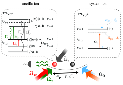
Figure 2: Implementation of the critical quantum sensor using two co-trapped ${}^{171}{\rm Yb}^{+}$ ions in a linear Paul trap which share a common vibrational (phonon) mode. The relevant energy levels are shown in the dotted boxes (not to scale). The system-ion is driven by two laser beams slightly detuned by $\delta_{\rm b}$ and $\delta_{\rm r}$ from the blue and red sideband transition respectively, realizing the Rabi Hamitonian, $\hat{H}_{R}$. The ancilla ion is also driven by two laser beams tuned to the carrier resonance and slightly detuned from the red sideband transition respectively. The annihilation of the phonon mode triggers the emission of multiple photons that are counted by a photon detector. Finally, an additional laser (of strength $\widetilde{\Omega}_{s}$) restores the internal state of the ancilla ion with a controllable rate, thereby accomplishing continuous phonon detection with near unit efficiency.

Measurement Scheme – A promising platform for the realization of our critical sensing scheme is based on the trapped-ion setup depicted in Fig. 2. We consider two trapped ions in a linear Paul trap sharing a quantized vibrational motion (phonon mode) which we assume is cooled down to the ground state. The two ions can be individually manipulated by lasers via single-ion addressability with focused laser beams [32] or via frequency space addressing with a crystal of mixed species [33]. As described in [34, 35, 36, 37], the Rabi Hamiltonian, $\hat{H}_{\rm R}$, can be implemented by driving the spin transition $\ket{\downarrow}\to\ket{\uparrow}$ of the system-ion with two travelling-wave laser beams with the same Rabi frequency, $\Omega_{0}$, and with frequencies $\omega_{I}+\omega_{\rm ph}-\delta_{\rm b}$ and $\omega_{I}-\omega_{\rm ph}-\delta_{\rm r}$; i.e, slightly detuned from the blue and red-sideband transition respectively. Here, $\omega_{I}$ is the frequency of the ionic spin transition, $\omega_{\rm ph}$ the phonon frequency and $\delta_{b(r)}\ll\omega_{\rm ph}$ is a small frequency offset. After moving to a suitable rotating-frame and performing an optical and a vibrational rotating-wave approximation (RWA), the Hamiltonian of the system-ion reads [38]

$$\hat{H}_{\rm R}=\frac{\delta_{\rm b}-\delta_{\rm r}}{2}\hat{c}^{\dagger}\hat{c}+\frac{\delta_{\rm r}+\delta_{\rm b}}{4}\hat{\sigma}_{z}+\frac{\eta_{\rm LD}\Omega_{0}}{2}\hat{\sigma}_{x}(\hat{c}+\hat{c}^{\dagger}),$$ (6)

where $\eta_{\rm LD}=k/\sqrt{2m\omega_{\rm ph}}$ is the Lamb-Dicke parameter, with $m$ the ion mass and $k$ the magnitude of the laser wavevector along the direction of the quantized oscillation. Eq. (6) has exactly the same form as the Rabi Hamiltonian in Eq. (1), with the new set of parameters $\omega=(\delta_{\rm b}-\delta_{\rm r})/2$, $\Omega=(\delta_{\rm b}+\delta_{\rm r})/2$ and $\lambda=\eta_{\rm LD}\Omega_{0}/2$. All these parameters can be adjusted experimentally and thus allow for tuning of the system to the CP.

Our sensing proposal further requires controlled dissipation of the phonon mode and efficient continuous detection of the phonons, both of which can be achieved by the means of the ancilla-ion, cf. Fig. 1. In particular, we assume that the ancilla-ion is driven by two additional laser beams: one slightly detuned from the red phonon sideband, $\Delta_{w}=-\omega_{\rm ph}-\omega$, and a second one on resonance with the carrier interaction, $\Delta_{s}=0$. The first laser drives the cooling transition $|g\rangle|n\rangle\longleftrightarrow|g\rangle|n-1\rangle$ with strength $\sqrt{n}\eta_{\rm LD}^{(2)}\Omega_{w}$, where $\eta_{\rm LD}^{(2)}$ is the Lamb-Dicke parameter of the ancilla-ion; the latter realises the strong transition $|e\rangle|n\rangle\longleftrightarrow|d\rangle|n\rangle$ with Rabi frequency $\Omega_{s}$. In the regime $\Omega_{s},\Gamma_{s}\gg\Omega_{w},\Gamma_{w}$, where $\Gamma_{s(w)}$ is the spontaneous emission rate of the strong (weak) transition $|d\rangle\rightarrow|e\rangle$ $(|e\rangle\rightarrow|g\rangle)$, a controllable dissipation rate $\kappa\approx\Gamma_{s}\Omega_{w}^{2}/\Omega_{s}^{2}$ is realized [38], where each phonon annihilation is accompanied with the emission of a significant number of photons from the strongly driven transition which in turn are collected and counted by a photon detector with efficiency $\epsilon$. This results in the efficient continuous measurement of the phonon mode characterized by the enhancement factor [38]

$$N_{\rm ph}\equiv\frac{\text{detected photon \#}}{\text{annihilated phonon \#}}\approx\epsilon\frac{\Gamma_{s}}{\Gamma_{w}}.$$ (7)

Quantitatively, the conditional dynamics of the system and ancilla ions interacting with the phonon mode can be described by a stochastic master equation [31] of the unnormalized joint state [38]

$$d\tilde{\rho}_{c}= \left(-i[\hat{H}_{R}+\hat{H}_{\rm{a}},\tilde{\rho}_{c}]\right.$$ (8)

$$\left.-\frac{\Gamma_{w}}{2}\{|e\rangle\langle e|,\tilde{\rho}_{c}\}+\Gamma_{w}|g\rangle\langle e|\tilde{\rho}_{c}|e\rangle\langle g|\right.$$

$$\left.-\frac{\Gamma_{s}}{2}\{|d\rangle\langle d|,\tilde{\rho}_{c}\}+(1-\epsilon)\Gamma_{s}|e\rangle\langle d|\tilde{\rho}_{c}|d\rangle\langle e|\right)dt$$

$$+(\epsilon\Gamma_{s}dt|e\rangle\langle d|\tilde{\rho}_{c}|d\rangle\langle d|-\tilde{\rho_{c}})dN(t),$$

where $\hat{H}_{\rm a}=\Omega_{s}(|d\rangle\langle e|+|e\rangle\langle d|)+\eta_{\rm LD}^{(2)}\Omega_{w}(|e\rangle\langle g|\hat{c}+|g\rangle\langle e|\hat{c}^{{\dagger}})$ is the Hamiltonian of the ancilla ion in the appropriate rotating-frame. Notice that although in Eq. (8) we assume that the state $|e\rangle$ relaxes directly to $|g\rangle$, cf. Fig. 1, in reality this re-initiliazation transition might be implemented through an additional excited level as shown in Fig. 2 and explained below. Here $dN(t)$ is a stochastic Poisson increment which, similar to the ideal case of perfect detection, can take two values: if there is a photon detected, $dN(t)=1$ with a modified probability $\tilde{p}_{1}=\epsilon\Gamma_{s}dt{\rm Tr}\{\rho_{c}\}$, where $\rho_{c}\equiv\tilde{\rho}_{c}/{\rm tr}(\tilde{\rho}_{c})$ is the normalized conditional density matrix, while if there is no photon detection $dN(t)=0$ with probability $\tilde{p}_{0}=1-\tilde{p}_{1}$. Taking the ensemble average over all conditional states and after elimination of the ancilla-ion leads to the definition of the joint system-ion–phonon state which evolves according to Eq. (2).

The significantly enhanced metrological precision via our measurement scheme is demonstrated in Fig. 3(a), which shows the FI for the estimation of the frequency of the phonon mode, $F_{\omega}(t)$, at various enhancement factors, $N_{\rm ph}$. As illustrated, increasing $N_{\rm ph}$ leads to larger FI and thus enhanced precision, which can in principle achieve the ideal precision for perfect photon detection. In the experimental relevant case of photon detector efficiency $\epsilon=0.01$ and $N_{\rm ph}\approx 80$, we perform a numerical finite-size scaling analysis for different experimentally accessible system sizes $\eta$ (see below), as shown in Fig. 3(c) where the perfect data collapse indicates that the $F_{\omega}(t)$ for $\epsilon_{\rm ph}<1$ follows a similar transient and long time behavior as in Eqs. (4) and (5). In the following we analyze a concrete experimental realization of our measurement scheme, shown in Fig. 1, and we examine its robustness against various experimental noise sources.

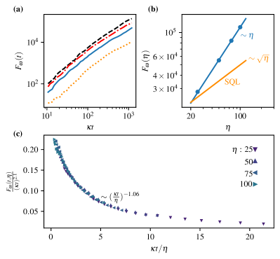
Figure 3: Fisher information for photon counting signals with imperfect photon detectors. (a) The behavior of the FI, $F_{\omega}(t)$, in comparison with the ideal case of $\epsilon=1$ (black dashed line) for $\epsilon=0.1$, $\Gamma_{s}/\Gamma_{w}=80\rightarrow N_{\rm ph}\approx 8$ (red dashed-dotted line); $\epsilon=0.01$, $\Gamma_{s}/\Gamma_{w}=80\rightarrow N_{\rm ph}\approx 0.8$ (blue solid line); $\epsilon=0.01$, $\Gamma_{s}/\Gamma_{w}=10\rightarrow N_{\rm ph}\approx 0.1$ (orange dotted line). In all curves $\Gamma_{w}=40$, $\Omega_{w}=14.3\Gamma_{w}$, $\Omega_{s}=2\Gamma_{s}$ and $\eta_{\rm LD}^{(2)}=0.07$. The above set of parameters for the ancilla-ion gives rise to a phonon dissipation rate $\kappa=1.5\times 10^{-3}\Gamma_{w}$. The system-ion is tuned to the dissipative CP and we choose $\omega=10\kappa$, $\eta=50$. (b) Long time behavior of the achieved FI with respect to the effective system size $\eta$ (blue line). For comparison we plot the scaling of FI that corresponds to SQL [10] (orange line). (c) Finite size scaling analysis of $F_{\omega}(t)$ averaged over $10^{4}$ trajectories for the case of $\epsilon=0.01$ and $\Gamma_{s}/\Gamma_{w}=80$. The remaining parameters are the same as in Fig.  3(a). Parameters for all panels are chosen from realistic experimental values (see main text).

Experimental implementation – Various ion species can be used for implementing our measurement scheme, and here, as a concrete example, we consider ${}^{171}{\rm Yb}^{+}$ as the ancilla-ion, whose internal level structure is shown in Fig. 2. We choose from the ground ${}^{2}S_{1/2}$ manifold the hyperfine states $|g\rangle\equiv|{F}=0,{m_{F}}=0\rangle$ and $|e\rangle\equiv|{F}=1,{m_{F}}=0\rangle$ to implement the phonon sideband cooling, cf. Fig. 1, with a frequency difference $\Delta_{\rm HFS}\approx 2\pi\times 12.6{\rm GHz}$, while the readout state is chosen as $|d\rangle\equiv|{F}=0,{m_{F}}=0\rangle$ from the excited ${}^{2}P_{1/2}$ manifold. The cooling transition $|g\rangle|n\rangle\rightarrow|e\rangle|n-1\rangle$ can be accomplished either by microwave in resonance with the red phonon sideband, or by stimulated Raman transition at a two-photon detuning $\Delta_{\rm HFS}-\omega_{\rm ph}$ [39]. The strong cycling transition $\ket{e}\longleftrightarrow$ $\ket{d}$, with a spontaneous emission rate $\Gamma_{s}=2\pi\times 19.6{\rm MHz}$ of the ${}^{2}P_{1/2}$ manifold, can be driven by a laser beam at $369.5{\rm nm}$ with adjustable Rabi frequency $\Omega_{s}$, cf. Fig. 2. Since the $\ket{d}\to\ket{g}$ emission channel is forbidden by dipole selection rules, an additional laser of strength $\widetilde{\Omega}_{s}$, detuned by $\Delta$ from the $\ket{e}\to\ket{m}\equiv$ ${}^{2}P_{1/2}|{F}=1,{m_{F}}=0\rangle$ transition, induces an effective decay $|e\rangle\rightarrow|g\rangle$ at an adjustable rate [40],

$$\Gamma_{w}\approx\frac{\Gamma_{s}}{2}\frac{(2\widetilde{\Omega}_{s}/\Gamma_{s})^{2}}{1+(\frac{2\widetilde{\Omega}_{s}}{\Gamma_{s}})^{2}+(\frac{2\Delta}{\Gamma_{s}})^{2}}.$$ (9)

As described in [37], the two states of the ground state manifold of a second ${}^{171}{\rm Yb}^{+}$ ion can be chosen as the qubit states, which together with the spatial motion of the ion along one of its principle axis, with frequency $\omega_{{\rm ph}}=2\pi\times 2.35{\rm MHz}$, provide the two degrees of freedom for implementing the Rabi Hamiltonian. A typical set of experimental parameters is $\omega\approx 2\pi\times 2{\rm kHz}$ and $(\eta_{\rm LD}\Omega_{0})_{\rm max}\approx 2\pi\times 20{\rm kHz}$ with $\eta_{\rm LD}=0.07$. Therefore, effective system size of $\eta\lesssim 100$ can be easily achieved. To achieve even larger $\eta>100$, a stronger Rabi frequency $\Omega_{0}$ is required to tune the system to the CP, which may ultimately break the vibrational RWA and modifies the resulting Hamiltonian of the system-ion. This can be overcome by suppressing the corresponding carrier transition, e.g, by using standing wave configuration [35] or exploiting the ac Stark shift of travelling waves [41] to implement the sideband transitions, which allows for exploring the critical physics close to the thermodynamic limit .

For the implementation of the ancilla-enhanced continuous readout, we assume that $\eta_{\rm LD}^{(2)}\Omega_{w}\approx 2\pi\times 150{\rm kHz}$ with $\eta_{\rm LD}^{(2)}=0.07$ and $\Gamma_{w}$ can be adjusted to $\Gamma_{w}=\Gamma_{s}/80=2\pi\times 245{\rm kHz}$. These realistic parameters result in a phonon dissipation rate $\kappa=2\pi\times 200{\rm Hz}$ with $N_{\rm ph}\approx 80$ [38] which, remarkably, allow for a clear demonstration of the criticality enhanced precision scaling as shown in Fig. 3(b).

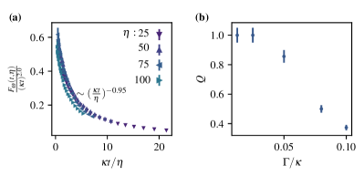
Figure 4: (a) Finite size scaling analysis of $F_{\omega}(t)$ for $\epsilon=1$ including noise with $\Gamma_{\rm dph}=\kappa/200$ and $\Gamma_{\rm m}=\Gamma_{\rm h}=\Gamma_{\rm c}=\kappa/10$. The rest of the parameters are the same as in Fig. 2. Each data point represents an average over $5\times 10^{3}$ independent trajectories. (b) The quality of data collapse, $Q$, in comparison with the noiseless scenario. For $\Gamma\leq\kappa/40$, the Fisher information, $F_{\omega}(t)$, follows the same scaling behaviour as predicted for the noiseless case

.

Effects of noise – The main experimental noise sources that may impact the performance of our sensing scheme are (i) spin decoherence of the system-ion at a rate $\Gamma_{\rm dph}$ capturing also the frequency noise of the laser, (ii) motional decoherence of the phonon mode at a rate $\Gamma_{\rm m}$, and (iii) motional diffusion of the phonon mode mainly caused by photon recoil in the strong transition of the ancila-ion which, in the side-band resolved regime, results in effective phonon heating and cooling, at a rate $\Gamma_{\rm h}$ and $\Gamma_{\rm c}$ respectively. Note that these imperfections affect neither the effective dissipation rate of the phonon mode $\kappa$ nor the highly efficient ancilla-assisted continuous phonon counting. Consequently, for the sake of numerical efficiency, we examine the effect of noise under the assumption of perfect photon detection efficiency $\epsilon=1$. In this case the SME of the unnormalised system-ion–phonon state reads

$$d\tilde{\rho}_{c}= \left(-i[\hat{H}_{R},\tilde{\rho}_{c}]+\Gamma_{\rm dph}\mathcal{L}[\hat{\sigma}_{z}]+\Gamma_{\rm m}\mathcal{L}[\hat{c}^{\dagger}\hat{c}]\right.$$ (10)

$$\left.+\Gamma_{\rm h}\mathcal{L}[\hat{c}^{\dagger}]+\Gamma_{\rm c}\mathcal{L}[\hat{c}]-\kappa\{\hat{c}^{\dagger}\hat{c},\tilde{\rho}_{c}\}\right)dt$$

$$+(2\kappa\hat{c}\tilde{\rho}_{c}\hat{c}^{\dagger}-\tilde{\rho}_{c})dN(t)$$

where $\mathcal{L}[\hat{x}]\equiv\hat{x}\tilde{\rho}_{c}\hat{x}^{\dagger}-\frac{1}{2}\{\hat{x}^{\dagger}\hat{x},\tilde{\rho}_{c}\}$. We take typical experimental numbers $\Gamma_{\rm dph}=2\pi\times 1{\rm Hz}$ and $\Gamma_{\rm m}=\Gamma_{\rm h}=\Gamma_{\rm c}=\Gamma=2\pi\times 20{\rm Hz}$ [37, 42]. Consequently, fixing $\Gamma_{\rm dph}=\kappa/200$ and $\Gamma=\kappa/10$ while keeping the rest of the parameters the same as Fig. 2, we show the resulting FI $F_{\omega}(t)$ in Fig. 4(a). The results indicate that although the various noise sources degrades the perfect data collapse, a scaling behaviour similar to the noiseless case persists. The quality of the data collapse can be quantified by the dimensionless quality factor $Q$ [43] that captures the mean relative spread among different sets of data [38]. As shown in Fig. 4(b), $Q\sim 1$ persists for small decoherence rate, indicating that the associated Fisher information follows the same scaling behaviour as the noiseless case. This demonstrates the feasibility of our sensing scheme under realistic experimental imperfections.

Conclusions – Our study proposes and analyzes an experimental implementation of a criticality-enhanced sensor using a finite-component critical open sensor with single trapped ions, and demonstrates its feasibility through continuous measurement. A key innovation of our implementation is the use of a co-trapped ancilla ion as a detection module, which provides highly efficient continuous phonon counting. Our implementation is also robust against various sources of noise, allowing for a clear demonstration of criticality-enhanced precision scaling well beyond the standard quantum limit. These results pave the way for practical applications of driven-dissipative critical systems as sensors, and hold the potential for significant advancements in sensing technology.

Acknowledgements –This work was supported by the Eu project QuMicro (Grant No. 01046911) and the ERC Synergy grant HyperQ (grant no 856432). We acknowledge support by the state of Baden-Württemberg through bwHPC and the German Research Foundation (DFG) through grant no INST 40/575-1 FUGG (JUSTUS2 cluster). Part of the numerical simulations wereperformed using the QuTiP library [44].

I Realization of the phonon detector module

In this section we discuss in detail the implementation of the phonon detector module with the help of the ancilla-ion, which has an internal ladder-type three-level structure as shown in Fig. 1. Neglecting the system-ion, the Hamiltonian for the internal transition and the external motion (i.e., the phonon mode) of the ancilla reads ($\hbar=1$)

$$\hat{H}_{\rm{a}}^{(I)}(t)=\omega_{\rm ph}\hat{c}^{\dagger}\hat{c}+\sum_{i=g,e,d}\omega_{i}|i\rangle\langle i|+\Omega_{w}(|e\rangle\langle g|+\text{h.c.})\left[e^{i(k_{w}\hat{x}-\omega_{w}t-\phi_{w})}+\text{h.c.}\right]+\Omega_{s}(|d\rangle\langle e|+\text{h.c.})\left[e^{i(k_{s}\hat{x}-\omega_{s}t-\phi_{s})}+\text{h.c.}\right],$$ (11)

where the weak (strong) laser beam is characterised by the Rabi frequency $\Omega_{w(s)}$, frequency $\omega_{w(s)}$, wavevector $k_{w(s)}$ and phase $\phi_{w(s)}$. Here $\hat{x}=x_{0}(\hat{c}+\hat{c}^{\dagger})$ is the ancilla-ion position operator, with $x_{0}=1/\sqrt{2\omega_{\rm ph}m_{\rm{a}}}$ and $m_{\rm{a}}$ the mass of the ion. We assume that the Lamb-Dicke parameter of the two lasers $\eta_{w(s)}:=k_{w(s)}x_{0}$ are the same and denote them as $\eta_{\rm LD}^{(2)}$. Moving to a frame rotating with respect to $\hat{H}_{0}=\omega_{\rm ph}\hat{c}^{\dagger}\hat{c}+(\omega_{e}-\omega_{g})|e\rangle\langle e|+(\omega_{d}-\omega_{g})|d\rangle\langle d|$, the Hamiltonian Eq. (11) takes the form

$$\hat{H}_{\rm{a}}(t) =\Omega_{w}(|e\rangle\langle g|e^{i(\omega_{e}-\omega_{g})t}+\text{h.c.})\left[e^{i(\eta_{\rm LD}^{(2)}(\hat{c}e^{-i\omega_{\rm ph}t}+\hat{c}^{\dagger}e^{i\omega_{\rm ph}t})-\omega_{w}t-\phi_{w})}+\text{h.c.}\right]$$ (12)

$$+\Omega_{s}(|d\rangle\langle e|e^{i(\omega_{d}-\omega_{e})t}+\text{h.c.})\left[e^{i(\eta_{\rm LD}^{(2)}(\hat{c}e^{-i\omega_{\rm ph}t}+\hat{c}^{\dagger}e^{i\omega_{\rm ph}t})-\omega_{s}t-\phi_{s})}+\text{h.c.}\right].$$

In the Lamb-Dicke regime $\eta\sqrt{\langle(\hat{c}+\hat{c}^{\dagger})^{2}\rangle}\ll 1$ we have

$$e^{\eta_{\rm LD}^{(2)}(\hat{c}e^{-i\omega_{\rm ph}t}+\hat{c}^{\dagger}e^{i\omega_{\rm ph}t})}\approx\mathcal{I}+\eta_{\rm LD}^{(2)}(\hat{c}e^{-i\omega_{\rm ph}t}+\hat{c}^{\dagger}e^{i\omega_{\rm ph}t}).$$ (13)

We can tune the two laser frequencies such that the weak laser drives resonantly the red phonon sideband of the $\ket{g}\to\ket{e}$ transition, $(\omega_{e}-\omega_{g})-\omega_{w}=\omega_{\rm ph}$; while the strong laser drives resonantly the carrier transition $\ket{g}\to\ket{d}$, $(\omega_{d}-\omega_{e})-\omega_{s}=0$. After choosing $\phi_{s}=\phi_{w}=0$, we perform an optical rotating-wave approximation (RWA) by neglecting terms rotating at frequency $\sim(\omega_{e}-\omega_{g})+\omega_{w}$, $\sim(\omega_{d}-\omega_{e})+\omega_{s}$ and a vibrational RWA where we neglect terms rotating at frequency $\sim\omega_{\rm ph}$. As a result, we obtain

$$\hat{H}_{\rm{a}}=\Omega_{s}(|d\rangle\langle e|+|e\rangle\langle d|)+\eta_{\rm LD}^{(2)}\Omega_{w}(|e\rangle\langle g|\hat{c}+|g\rangle\langle e|\hat{c}^{{\dagger}}).$$ (14)

for the Hamiltonian of the trapped ancilla-ion.

The quantum state of the ancilla-ion $\rho_{\rm{a}}$ (including both the internal transition and the external motion) evolves according to the LME

$$\frac{d\rho_{\rm{a}}}{dt}=-i[\hat{H}_{\rm{a}},\rho_{\rm{a}}]+\Gamma_{s}\left(|e\rangle\langle d|\rho_{\rm{a}}|d\rangle\langle e|-\frac{1}{2}\{|d\rangle\langle d|,\rho_{\rm{a}}\}\right)+\Gamma_{w}\left(|g\rangle\langle e|\rho_{\rm{a}}|e\rangle\langle g|-\frac{1}{2}\{|e\rangle\langle e|,\rho_{\rm{a}}\}\right).$$ (15)

To visualize such an evolution, in Fig. 5(a) we plot the phonon mode occupation in the appropriate parameter regime see below, which demonstrates an exponential decay with time at an effective dissipation rate $\kappa$. To acquire an understanding, let us relate the effective decay to the microscopic parameters $\Omega_{s}$, $\Gamma_{s}$, $\Gamma_{w}$. We can divide one full cooling cycle $|g\rangle|n\rangle\rightarrow|g\rangle|n-1\rangle$, where $|n\rangle$ denotes the phonon occupation number, into different elementary transitions. First, for small enough $\Gamma_{w}$, the event $|g\rangle|n\rangle\rightarrow|e\rangle|n-1\rangle$ defines the transition from the dark to the bright state of the ancilla ion at a characteristic timescale $T_{1}\approx\Omega_{s}^{2}/(\Omega_{w}^{2}\Gamma_{s})$ [28]. The inverse, undesired transition $|e\rangle|n-1\rangle\rightarrow|g\rangle|n\rangle$, with a characteristic timescale $T_{2}\approx(\Gamma_{s}^{2}+\Omega_{s}^{2})T_{1}/\Gamma_{s}^{2}$, restores the initial state of the ancilla-ion but without any phonon annihilation. As a result, to realize an effective dissipation of the phonon mode, we require that the spontaneous emission $|e\rangle|n-1\rangle\rightarrow|g\rangle|n-1\rangle$ happens at a timescale $1/\Gamma_{w}\equiv T_{3}\ll T_{2}$. The time of a complete cooling cycle is given by $1/\kappa\equiv T_{c}\approx T_{1}+T_{3}\approx T_{1}$ as we are in the regime where $\Omega_{s}\gg\Omega_{w}$. Such analytical understanding is confirmed by the numerical simulation shown in Fig. 5(b), where we plot the dependence of the effective dissipation rate $\kappa$ of the phonons with respect to the different parameters of our model.

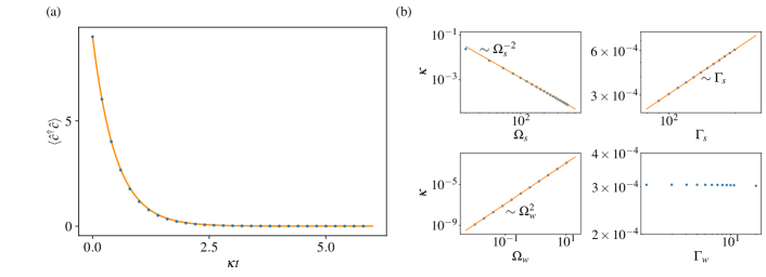
Figure 5: Induced dissipation of the bosonic mode via a three level ancilla-ion. a) Comparison of the evolution of the phonon’s excitation between an induced dissipation via an ancilla-ion with $\Gamma_{w}=40$, $\Omega_{w}=14.3\Gamma_{w}$, $\Gamma_{s}=80\Gamma_{w}$, $\Omega_{s}=2\Gamma_{s}$ and $\eta_{\rm LD}^{(2)}=0.07$ (blue dotted line) and a direct dissipation with $\kappa=1.5\times 10^{-3}\Gamma_{w}$ (orange solid line). b) Dependence of the induced dissipation rate, $\kappa$, with respect to different adjustable parameters in our system. The plots indicate that $\kappa\sim\Omega_{s}^{2}/(\Omega_{w}^{2}\Gamma_{s})$ as expected from our physical understanding.

II Trapped-ion implementation of the open Rabi model

Here, we discuss the implementation of the open Rabi model as presented schematically in Fig. 1. The system-ion is co-trapped with the ancilla-ion analyzed in Appendix I, and is driven by two travelling-wave laser beams of the same Rabi frequency, $\Omega_{0}$, and Lamd-Dicke parameter, $\eta_{\rm LD}$. As a result the Hamiltonian of the total system reads

$$\hat{H}_{\rm tot}^{(I)}(t)=\hat{H}_{\rm{a}}^{(I)}(t)+\hat{H}_{\rm{s}}^{(I)}(t),$$ (16)

where $\hat{H}_{\rm{s}}^{(I)}(t)=\frac{\omega_{I}}{2}\hat{\sigma}_{z}+\sum_{j}\frac{\Omega_{0}}{2}\hat{\sigma}_{x}\left(e^{i\eta_{\rm LD}(\hat{c}+\hat{c}^{\dagger})-\omega_{j}t-\phi_{j}}+\text{h.c.}\right)$ and $\hat{\sigma}_{z,x}$ are the Pauli matrices referring to the system-ion. In the rotating frame with respect to $\tilde{H}_{0}=\omega_{\rm ph}\hat{c}^{\dagger}\hat{c}+(\omega_{e}-\omega_{g})|e\rangle\langle e|+(\omega_{d}-\omega_{g})|d\rangle\langle d|+\frac{\omega_{I}}{2}\hat{\sigma}_{z}$, following similar approximations as before by choosing $\omega_{1}=\omega_{I}+\omega_{\rm ph}-\delta_{\rm b}$, $\omega_{2}=\omega_{I}-\omega_{\rm ph}-\delta_{\rm b}$, $\phi_{1}=\phi_{2}=3\pi/2$, $\omega_{s}=(\omega_{d}-\omega_{g})$, $(\omega_{e}-\omega_{g})-\omega_{w}=\omega_{\rm ph}+(\delta_{\rm b}-\delta_{\rm b})/2$ we arrive at

$$\hat{H}_{\rm tot}^{(I)}(t) =\Omega_{s}(|d\rangle\langle e|+|e\rangle\langle d|)+\eta_{\rm LD}^{(2)}\Omega_{w}(|e\rangle\langle g|\hat{c}e^{i\frac{\delta_{\rm b}-\delta_{\rm r}}{2}t}+|g\rangle\langle e|\hat{c}^{{\dagger}}e^{-i\frac{\delta_{\rm b}-\delta_{\rm r}}{2}t})$$

$$-\frac{\Omega_{0}\eta_{\rm LD}}{2}(\hat{\sigma}_{+}e^{i\frac{\delta_{\rm b}+\delta_{\rm r}}{2}t}+\text{h.c})(\hat{c}^{\dagger}e^{i\frac{\delta_{\rm b}-\delta_{\rm r}}{2}t}+\text{h.c}).$$ (17)

In the frame rotating with $H^{{}^{\prime}}_{0}=\frac{\delta_{\rm b}-\delta_{\rm r}}{2}\hat{c}^{\dagger}\hat{c}+\frac{\delta_{\rm r}+\delta_{\rm b}}{4}\hat{\sigma}_{z}$, the evolution of the full model is governed by the LME

$$\frac{d\rho}{dt}=-i[\hat{H}_{\rm{s}}+\hat{H}_{\rm{a}},]+\Gamma_{s}\left(|e\rangle\langle d|\rho|d\rangle\langle e|-\frac{1}{2}\{|d\rangle\langle d|,\rho\}\right)+\Gamma_{w}\left(|g\rangle\langle e|\rho|e\rangle\langle g|-\frac{1}{2}\{|e\rangle\langle e|,\rho\}\right),$$ (18)

which correctly implements the LME (2) of the open Rabi model as illustrated in Fig. 6.

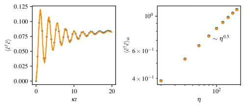
Figure 6: Trapped-ion realisation of the open Rabi model. a) Dynamics of the phonon’s excitation in the open Rabi model as implemented with the help of an ancilla-ion and evolved according to Eq. (18) (blue-dotted line) and Eq. (2) (orange solid line). Parameters: $\eta=50$, $\omega=0.6$; the rest kept the same as Fig. 5 . b) Steady state occupation of the bosonic mode with respect to different system sizes, $\eta$, as calculated from Eq.(18) (blue-dotted line) and Eq.(2) (orangle-dotted line). The excellent agreement between the two lines in both plots demonstrates the accurate implementation of the open Rabi model in our set-up.

III Enhanced Continuous Phonon Detection

In this section we discuss the highly efficient continuous measurement of the phonon mode accomplished by the use of the ancilla-ion. Adopting the physical picture developed in Appendix II, it is clear that once an event $|g\rangle|n\rangle\rightarrow|e\rangle|n-1\rangle$ occurs, the strongly driven transition $|e\rangle\leftrightarrow|d\rangle$ of the ancilla-ion leads to the emission of photons at a rate $\Gamma_{\rm ph}=\Gamma_{s}\times P_{\rm ex}\approx\frac{\Gamma_{s}}{2}\frac{(2\Omega_{s}/\Gamma_{s})^{2}}{1+(2\Omega_{s}/\Gamma_{s})^{2}}$, where $P_{\rm ex}$ is the probability to find the ancilla-ion in the $|d\rangle\langle d|$ state. The characteristic timescale for restoring the population, $|e\rangle\rightarrow|g\rangle$, is $T_{2}=1/\Gamma_{w}$. As a result, during a full cooling cycle $|g\rangle|n\rangle\rightarrow|g\rangle|n-1\rangle$ there are $N_{\rm em}=T_{2}\times\Gamma_{\rm ph}\approx\Gamma_{s}/\Gamma_{w}$ photons emitted and $N_{\rm ph}=\epsilon N_{\rm em}$ photons detected which lead to the definition of the enhancement factor as in Eq. (7) of the main text. As a simple demonstration, let us again neglect the system-ion, and consider the enhanced measurement of a single vibrational phonon mode occupying an excited Fock state. The conditional evolution of the phonon mode is given by a stochastic master equation similarly to Eq. (8) of the main text. As shown in Fig. 7, for any photon detector of efficiency, $\epsilon$, we can implement almost perfect detection of the phonon mode by appropriate engineer of the parameters for the internal transitions the ancilla.

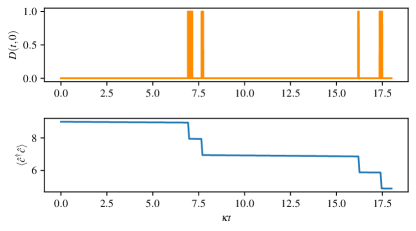
Figure 7: Conditional evolution of the damped bosonic mode of the trap as implemented with the help of an ancilla-ion where each annihilated phonon is accompanied with the emission and detection of lots of photons. Upper panel: The photon-detection signal, $D(t,0)$, of a detector with efficiency $\epsilon=0.5$; Lower panel: the conditional evolution of the damped mode as exemplified by the bosonic mode occupation $\langle\hat{c}^{\dagger}\hat{c}\rangle$. The dynamics of a single trajectory associated with the corresponding detected signal is the same as the ideal case of perfect photon detection. Parameters: $\Gamma_{w}=40$, $\Omega_{w}=14.3\Gamma_{w}$, $\Omega_{s}=2\Gamma_{s}=160\Gamma_{w}$ and $\eta_{\rm LD}^{(2)}=0.07$.

IV Quality of the Scaling Collapse

The finite-size scaling analysis is a powerful numerical method to extract the relevant exponents of continuous phase transitions. Consider a general quantity $\mathcal{A}$ dependent on two parameters $h$ and $L$ according to

$$\mathcal{A}(h,L)=h^{a}f(h/L^{b}).$$ (19)

Depending on the nature of the model system, $\mathcal{A}$, $L$ and $h$ can refer to different quantities. For example, $\mathcal{A}$ might refer to the magnetization of the Ising spin chain, with $h$ being the inverse of the transverse magnetic field and $L$ the length of the chain. In our case, $\mathcal{A}$ refers to the Fisher information $F_{\omega}(t,\eta)$, with $L$ and $h$ being the system size $\eta$ and the evolution time $t$ respectively. From Eq. (19), it is clear that if we plot $\mathcal{A}h^{-a}$ against $h/L^{b}$ for different values of $L$ and $h$, all the curves collapse onto a single. Therefore, we can determine the unknown exponents $a$ and $b$ by numerical fitting of the data to Eq. (19) and find the best scaling collapse.

We can define appropriate measure of the quality of the data collapse to remove subjectiveness of the approach. If the scaling function $f(x)$ is known, we can define the measure [43]

$$\mathcal{M}_{kn}(a,b)=\sqrt{\frac{1}{N}\sum_{ij}\left(\frac{\mathcal{A}({L_{i},h_{j}})h_{j}^{-a}-f(L_{i}^{-b}h_{j})}{f(L_{i}^{-b}h_{j})}\right)^{2}}$$ (20)

which is minimized by the optimal $a$ and $b$, with $N$ the total number of data points. Notice that in Eq. (20) the division with respect to the scaling function $f(x)$ is essential—otherwise $\mathcal{M}_{kn}$ can be minimized for small values of the numerator which not necessarily indicates a good collapse.

In the general case the scaling function $f(x)$ is not known. We can interpolate $f(x)$ via any set of data points corresponding to a specific $L$. Denoting the different sets via the subscript $p$, we can measure the quality of the data collapse by comparing the data points of pairs of sets $p_{1,2}$ in their overlapping regions and summing up all the contribution,

$$\mathcal{M}(a,b)=\sqrt{\frac{1}{N}\sum_{p}\sum_{i\neq p}\sum_{j,\rm{ov}}\left(\frac{\mathcal{A}({L_{i},h_{j}})h_{j}^{-a}-\mathcal{E}_{p}(L_{i}^{-b}h_{j})}{\mathcal{E}_{p}(L_{i}^{-b}h_{j})}\right)^{2}},$$ (21)

where $\mathcal{E}_{p}(x)$ is the interpolation function based on the basis set-$p$ and $N$ is the total number of points in all overlapping regions. Here, the innermost index $j$ runs over the overlapping region of the set-$p$ and another set-$i$. It is clear that $\mathcal{M}\geq 0$ with the zero lower bound achieved only in case of perfect data collapse. As a result, it can be used via the variational principle for an automatic and objective extrapolation of the relevant critical exponents.

For our case, in order to examine the quality of the finite-size scaling analysis for different decoherence rates, as shown in Fig. 3(b) in the main text, we introduce the quality factor

$$Q=\frac{\mathcal{M}^{F}_{\rm id}}{\mathcal{M}^{F}},$$ (22)

where $\displaystyle\mathcal{M}^{F}=\mathcal{M}(2,1)=\sqrt{\frac{1}{N}\sum_{p}\sum_{i\neq p}\sum_{j,\rm{ov}}\left(\frac{F(t_{j}\eta_{i})t_{j}^{2}-\mathcal{E}_{p}(\eta_{i}t_{j})}{\mathcal{E}_{p}(\eta_{i}t_{j})}\right)^{2}}$ is the measure of the data collapse, and $\mathcal{M}^{F}_{\rm id}$ refers to the measure of the ideal noiseless case.

References

- Zanardi et al. [2008] P. Zanardi, M. G. A. Paris, and L. Campos Venuti, Quantum criticality as a resource for quantum estimation, Phys. Rev. A 78, 042105 (2008).
- Tsang [2013] M. Tsang, Quantum transition-edge detectors, Phys. Rev. A 88, 021801 (2013).
- Rams et al. [2018] M. M. Rams, P. Sierant, O. Dutta, P. Horodecki, and J. Zakrzewski, At the limits of criticality-based quantum metrology: Apparent super-heisenberg scaling revisited, Phys. Rev. X 8, 021022 (2018).
- Fernández-Lorenzo and Porras [2017] S. Fernández-Lorenzo and D. Porras, Quantum sensing close to a dissipative phase transition: Symmetry breaking and criticality as metrological resources, Phys. Rev. A 96, 013817 (2017).
- Garbe et al. [2020] L. Garbe, M. Bina, A. Keller, M. G. A. Paris, and S. Felicetti, Critical quantum metrology with a finite-component quantum phase transition, Phys. Rev. Lett. 124, 120504 (2020).
- Candia et al. [2021] R. D. Candia, F. Minganti, K. V. Petrovnin, G. S. Paraoanu, and S. Felicetti, Critical parametric quantum sensing, (2021), arXiv:2107.04503 [quant-ph] .
- Heugel et al. [2019] T. L. Heugel, M. Biondi, O. Zilberberg, and R. Chitra, Quantum transducer using a parametric driven-dissipative phase transition, Phys. Rev. Lett. 123, 173601 (2019).
- Chu et al. [2021] Y. Chu, S. Zhang, B. Yu, and J. Cai, Dynamic framework for criticality-enhanced quantum sensing, Phys. Rev. Lett. 126, 010502 (2021).
- Salado-Mejía et al. [2021] M. Salado-Mejía, R. Román-Ancheyta, F. Soto-Eguibar, and H. M. Moya-Cessa, Spectroscopy and critical quantum thermometry in the ultrastrong coupling regime, Quantum Science and Technology 6, 025010 (2021).
- Ilias et al. [2022] T. Ilias, D. Yang, S. F. Huelga, and M. B. Plenio, Criticality-enhanced quantum sensing via continuous measurement, PRX Quantum 3, 010354 (2022).
- Garbe et al. [2022] L. Garbe, O. Abah, S. Felicetti, and R. Puebla, Exponential time-scaling of estimation precision by reaching a quantum critical point, Phys. Rev. Res. 4, 043061 (2022).
- Ding et al. [2022] D.-S. Ding, Z.-K. Liu, B.-S. Shi, G.-C. Guo, K. Mølmer, and C. S. Adams, Enhanced metrology at the critical point of a many-body rydberg atomic system, Nat. Phys. 18, 1447 (2022).
- Salvia et al. [2022] R. Salvia, M. Mehboudi, and M. Perarnau-Llobet, Critical quantum metrology assisted by real-time feedback control (2022).
- Wineland et al. [1992] D. J. Wineland, J. J. Bollinger, W. M. Itano, F. L. Moore, and D. J. Heinzen, Spin squeezing and reduced quantum noise in spectroscopy, Phys. Rev. A 46, R6797 (1992).
- Huelga et al. [1997] S. F. Huelga, C. Macchiavello, T. Pellizzari, A. K. Ekert, M. B. Plenio, and J. I. Cirac, Improvement of frequency standards with quantum entanglement, Phys. Rev. Lett. 79, 3865 (1997).
- Giovannetti et al. [2004] V. Giovannetti, S. Lloyd, and L. Maccone, Quantum-enhanced measurements: Beating the standard quantum limit, Science 306, 1330 (2004).
- Baumann et al. [2010] K. Baumann, C. Guerlin, F. Brennecke, and T. Esslinger, Dicke quantum phase transition with a superfluid gas in an optical cavity, Nature 464, 1301 (2010).
- Klinder et al. [2015] J. Klinder, H. Keßler, M. Wolke, L. Mathey, and A. Hemmerich, Dynamical phase transition in the open dicke model, Proceedings of the National Academy of Sciences 112, 3290 (2015).
- Baden et al. [2014] M. P. Baden, K. J. Arnold, A. L. Grimsmo, S. Parkins, and M. D. Barrett, Realization of the dicke model using cavity-assisted raman transitions, Phys. Rev. Lett. 113, 020408 (2014).
- Rodriguez et al. [2017] S. R. K. Rodriguez, W. Casteels, F. Storme, N. Carlon Zambon, I. Sagnes, L. Le Gratiet, E. Galopin, A. Lemaître, A. Amo, C. Ciuti, and J. Bloch, Probing a dissipative phase transition via dynamical optical hysteresis, Phys. Rev. Lett. 118, 247402 (2017).
- Fitzpatrick et al. [2017] M. Fitzpatrick, N. M. Sundaresan, A. C. Y. Li, J. Koch, and A. A. Houck, Observation of a dissipative phase transition in a one-dimensional circuit qed lattice, Phys. Rev. X 7, 011016 (2017).
- Fink et al. [2017] J. M. Fink, A. Dombi, A. Vukics, A. Wallraff, and P. Domokos, Observation of the photon-blockade breakdown phase transition, Phys. Rev. X 7, 011012 (2017).
- Cai et al. [2022] M.-L. Cai, Z.-D. Liu, Y. Jiang, Y.-K. Wu, Q.-X. Mei, W.-D. Zhao, L. He, X. Zhang, Z.-C. Zhou, and L.-M. Duan, Probing a dissipative phase transition with a trapped ion through reservoir engineering, Chinese Phys. Lett. 39, 020502 (2022).
- Hempel et al. [2013] C. Hempel, B. P. Lanyon, P. Jurcevic, R. Gerritsma, R. Blatt, and C. F. Roos, Entanglement-enhanced detection of single-photon scattering events, Nature Photon. 7, 630 (2013).
- Wan et al. [2014] Y. Wan, F. Gebert, J. B. Wübbena, N. Scharnhorst, S. Amairi, I. D. Leroux, B. Hemmerling, N. Lörch, K. Hammerer, and P. O. Schmidt, Precision spectroscopy by photon-recoil signal amplification, Nat. Commun. 5, 3096 (2014).
- Leibfried et al. [2003] D. Leibfried, R. Blatt, C. Monroe, and D. Wineland, Quantum dynamics of single trapped ions, Rev. Mod. Phys. 75, 281 (2003).
- Hwang et al. [2018] M.-J. Hwang, P. Rabl, and M. B. Plenio, Dissipative phase transition in the open quantum rabi model, Phys. Rev. A 97, 013825 (2018).
- Plenio and Knight [1998] M. B. Plenio and P. L. Knight, The quantum-jump approach to dissipative dynamics in quantum optics, Rev. Mod. Phys. 70, 101 (1998).
- Cohen-Tannoudji et al. [1998] C. Cohen-Tannoudji, J. Dupont-Roc, and G. Grynberg, Atom-Photon Interactions: Basic Processes and Applications (1998).
- Carmichael [1993] H. Carmichael, An Open Systems Approach to Quantum Optics (Springer, Berlin, 1993).
- Wiseman and Milburn [2009] H. M. Wiseman and G. J. Milburn, Quantum Measurement and Control (Cambridge University Press, 2009).
- Linke et al. [2017] N. M. Linke, D. Maslov, M. Roetteler, S. Debnath, C. Figgatt, K. A. Landsman, K. Wright, and C. Monroe, Experimental comparison of two quantum computing architectures, Proceedings of the National Academy of Sciences 114, 3305 (2017).
- Negnevitsky et al. [2018] V. Negnevitsky, M. Marinelli, K. K. Mehta, H. Y. Lo, C. Flühmann, and J. P. Home, Repeated multi-qubit readout and feedback with a mixed-species trapped-ion register, Nature 563, 527 (2018).
- Pedernales et al. [2015] J. S. Pedernales, I. Lizuain, S. Felicetti, G. Romero, L. Lamata, and E. Solano, Quantum Rabi model with trapped ions, Sci. Rep. 5, 15472 (2015).
- Puebla et al. [2017] R. Puebla, M.-J. Hwang, J. Casanova, and M. B. Plenio, Probing the dynamics of a superradiant quantum phase transition with a single trapped ion, Phys. Rev. Lett. 118, 073001 (2017).
- Lv et al. [2018] D. Lv, S. An, Z. Liu, J.-N. Zhang, J. S. Pedernales, L. Lamata, E. Solano, and K. Kim, Quantum simulation of the quantum rabi model in a trapped ion, Phys. Rev. X 8, 021027 (2018).
- Cai et al. [2021] M. L. Cai, Z. D. Liu, W. D. Zhao, Y. K. Wu, Q. X. Mei, Y. Jiang, L. He, X. Zhang, Z. C. Zhou, and L. M. Duan, Observation of a quantum phase transition in the quantum Rabi model with a single trapped ion, Nat. Commun. 12, 1126 (2021).
- [38] See Supplemental Material for details.
- Blinov et al. [2004] B. B. Blinov, D. Leibfried, C. Monroe, and D. J. Wineland, Quantum computing with trapped ion hyperfine qubits, Quantum Information Processing 3, 45 (2004).
- Noek et al. [2013] R. Noek, G. Vrijsen, D. Gaultney, E. Mount, T. Kim, P. Maunz, and J. Kim, High speed, high fidelity detection of an atomic hyperfine qubit, Opt. Lett. 38, 4735 (2013).
- Jonathan et al. [2000] D. Jonathan, M. B. Plenio, and P. L. Knight, Fast quantum gates for cold trapped ions, Phys. Rev. A 62, 042307 (2000).
- Islam et al. [2014] R. Islam, W. C. Campbell, T. Choi, S. M. Clark, C. W. S. Conover, S. Debnath, E. E. Edwards, B. Fields, D. Hayes, D. Hucul, I. V. Inlek, K. G. Johnson, S. Korenblit, A. Lee, K. W. Lee, T. A. Manning, D. N. Matsukevich, J. Mizrahi, Q. Quraishi, C. Senko, J. Smith, and C. Monroe, Beat note stabilization of mode-locked lasers for quantum information processing, Opt. Lett. 39, 3238 (2014).
- Bhattacharjee and Seno [2001] S. M. Bhattacharjee and F. Seno, A measure of data collapse for scaling, J. Phys. A: Math. Gen.l 34, 6375 (2001).
- Johansson et al. [2013] J. Johansson, P. Nation, and F. Nori, Qutip 2: A python framework for the dynamics of open quantum systems, Comp. Phys. Comm. 184, 1234 (2013).