Multi-Class Explainable Unlearning
for Image Classification via Weight Filtering

Abstract

Machine Unlearning has recently been emerging as a paradigm for selectively removing the impact of training datapoints from a network. While existing approaches have focused on unlearning either a small subset of the training data or a single class, in this paper we take a different path and devise a framework that can unlearn all classes of an image classification network in a single untraining round. Our proposed technique learns to modulate the inner components of an image classification network through memory matrices so that, after training, the same network can selectively exhibit an unlearning behavior over any of the classes. By discovering weights which are specific to each of the classes, our approach also recovers a representation of the classes which is explainable by-design. We test the proposed framework, which we name Weight Filtering network (WF-Net), on small-scale and medium-scale image classification datasets, with both CNN and Transformer-based backbones. Our work provides interesting insights in the development of explainable solutions for unlearning and could be easily extended to other vision tasks.

1 Introduction

With the growing effectiveness of Deep Learning models and the emergence of large-scale datasets collected from the web, the community has been witnessing an increasing need to preserve user privacy and defend the “right to be forgotten” [8], i.e. having private data used for training deleted.

To respond to these needs, Machine Unlearning [31] solutions have been emerging to remove the trace left by one or more datapoints from a trained model. The base idea behind these approaches [5, 20, 4] is to “untrain” the model so as to remove the impact of unwanted datapoints and, ultimately, reach a set of weights which is most similar to that of a model trained without the unwanted data.

Figure 1: Comparison between single-class unlearning and the proposed single-round multi-class unlearning setting. Our approach can unlearn any class in a single untraining round and avoids the need of storing multiple models. WF-Net requires less computational resources and supports explainability by-design.

While removing one or more datapoints is crucial for addressing specific privacy concerns, the literature has also been recently investigating the removal of entire classes from a classification network [2, 29, 30]. This setting, which is far more complex in both computational and algorithmic terms, is needed when the entire class is a source of privacy leak (e.g., in a face recognition system) but also opens up new possibilities in terms of removing portions of the knowledge learned by the model when it is detrimental or not needed for a specific application scenario. Unfortunately, existing methods are limited to unlearning a single class and can not handle the unlearning of multiple classes in a single round. When the model needs to selectively forget more than one class, therefore, we are left with the only option of repeating the unlearning procedure for each class, which inevitably leads to higher computational requirements.

In this paper, we move a step forward and tackle the task of unlearning multiple classes in a single untraining round. The resulting model, at test time, can be instructed to behave as if it has been untrained on any class, without performing a specific untraining stage and without storing separate models. In comparison with single-class unlearning (Figure 1), therefore, we avoid the need of storing multiple models and performing multiple untraining rounds. To achieve this goal, we start from the observation that there exists a mapping between inner network components (e.g., convolutional filters in a CNN [19] or attentive projection in a ViT [11]) and output classes [37], and build a Weight-Filtering layer which can selectively turn on and off those inner components to accomplish the desired unlearning behavior on a class of choice. In practice, this is done by encapsulating existing network operators into the Weight-Filtering layer, therefore without the need of altering the network structure.

As training the proposed Weight-Filtering layers amounts to discovering the relationships between inner network components and output classes, beyond being effective for unlearning our approach also offers a representation that is explainable by-design. Experimentally, we validate the proposed approach on small-scale and medium-scale image classification datasets (MNIST, CIFAR-10, and ImageNet-1k) and demonstrate its applicability to a variety of image classification architectures, including both CNNs and ViTs, and to the more challenging case of unlearning without having access to the training set.

Contributions. To sum up, the contributions of this paper are as follows:

• We introduce a framework for unlearning multiple classes of an image classification network in a single untraining round. Compared to existing approaches, this allows for a significant reduction in computational requirements both at untraining and testing stages and provides increased flexibility.

• Our approach encapsulates inner network components like convolutional filters or attentive projections into Weight-Filtering layers, which can selectively turn on and off these inner components to achieve the desired unlearning behavior.

• As an additional benefit, our method implicitly discovers the underlying relationships between convolutional filters or attentive projections and output classes and therefore allows to obtain a representation that can be employed for explainability purposes.

• We perform experiments on small-scale and large-scale datasets for image classification, and test with CNN-based and ViT-based architectures. Our results demonstrate the effectiveness of the proposed approach.

2 Related Work

Machine Unlearning. The field of machine unlearning is a novel research area that seeks to develop techniques for erasing specific or sensitive data from pre-trained models. Ideally, a machine unlearning algorithm should be able to delete data from the model without requiring a complete retraining process. In this domain, Cao et al. [5] were among the pioneers in addressing the machine unlearning problem in the context of traditional machine learning algorithms, such as naive Bayes classifiers, support vector machines, and k-means clustering. However, this approach demonstrated only minor benefits compared to retraining from scratch and therefore is not well suited for the task of unlearning in deep neural networks.

More recently, some research efforts have been dedicated to the introduction of unlearning in the context of deep learning networks. While Izzo et al. [20] introduced a technique for removing datapoints from linear models, other works [40] have employed a data grouping during the training process, enabling seamless unlearning by restricting the impact of datapoints on the model learning process. Another approach [4], instead, is that of monitoring the impact of training datapoints on model parameters, thereby minimizing the amount of retraining required when a deletion request is received. However, all the aforementioned methods lead to high storage costs. A different line of research proposed to employ efficient partitioning of training data [14, 1]. Among these works, Ginart et al. [14] introduced a method for removing points from clustering by dividing the data into separate and independent partitions, eventually using a distinct trained model for each partition [1]. Another class of works [13, 12, 18] introduced the notion of influence functions [22] to unlearn a model from an individual datapoint. However, since the influence function is based on the first-order Taylor approximation, these unlearning algorithms are only accurate when the model undergoes small changes (e.g., erasing a datapoint from a large training dataset), thus limiting their applicability in real-world scenarios.

Recent unlearning paradigms involve the removal of entire classes from a pre-trained model [2, 29, 30, 36]. For example, Golatkar et al. [16] presented a technique for removing information from the intermediate layers of deep learning networks via stochastic gradient descent, that can be also extended to the final activation of the model [17]. To reduce the computational costs of these approaches, which degrade for larger datasets, in [15] a novel approach for mixed-privacy forgetting is introduced, showing scalability across various standard vision datasets. Differently from previous works, we propose to unlearn potentially any class of a pre-trained model in a single untraining stage, thus avoiding the need of saving multiple unlearned models.

Explainability. As neural networks have grown in size and complexity, it has become increasingly challenging to provide an interpretable account of how they operate. This has made explainability a crucial concern in recent years. In the context of neural networks, the terms “black box” and “white box” are frequently used to indicate the level of transparency of a given model. A white box neural network is a model whose internal workings are transparent and therefore they are explainable by design. This means that a white box model is designed to provide a clear and interpretable explanation [27, 41] of the process it used to generate its output.

On the other hand, a black box neural network is a model that lacks transparency in its internal workings, resulting in its output being difficult or impossible to explain. Therefore, for this type of network, there is a need for an external component that can provide interpretability [28, 34, 26, 3]. Over the past few years, a large variety of saliency-based methods have been developed to summarize where highly complex neural networks focus in an image to find evidence supporting their predictions [33, 38, 6]. On a similar line, some works [41, 10] also proposed novel visualization techniques that give insight into the function of intermediate feature layers, showing which patterns from the training set activate the feature map. While not explicitly designed for explainability, our approach can discover the underlying relationships of intermediate layers and output classes, thus providing an additional source for interpreting the internal representations of pre-trained models.

3 Proposed Method

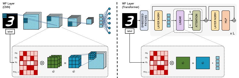
Figure 2: Application of Weighted-Filter layers for single-shot multiple class unlearning on CNN-based and ViT-based architectures.

3.1 Preliminaries

We consider a set of input data $\mathcal{D}=\{(x_{i},y_{i})\}_{i=1}^{n}$ with $n$ number of samples, where $x_{i}$ is the $i$-th sample and $y_{i}$ is the corresponding label belonging to a set of classes $\mathcal{C}$. Traditional training aims at identifying a set of weights $\hat{w}\in\mathcal{W}$ via an iterative update rule $w_{t+1}=w_{t}-g(w,x^{\prime})$, where $g(\cdot,x^{\prime})$ is a stochastic gradient of a fixed loss function. Once the model has reached convergence and given a set of datapoints $\mathcal{D}_{f}$ drawn from the same distribution of $\mathcal{D}$, machine unlearning aims at identifying an update to $\hat{w}$ in the form

$$\hat{w}_{t+1}=\hat{w}_{t}+g(z^{\prime}_{f}),\text{with }\hat{w}_{0}:=\hat{w}\text{ and }z^{\prime}_{f}\sim\mathcal{D}_{f}$$ (1)

so that $\mathcal{D}_{f}$ is to be unlearned. In other words, the final set of weights of the unlearned model should be close to a model trained from scratch on $\mathcal{D}\setminus\mathcal{D}_{f}$. Depending on the use case, $\mathcal{D}_{f}$ can be conceived as containing a single datapoint (i.e., item removal), a group of data with similar features or labels (i.e., feature removal), or an entire class (class removal) [31].

Class removal. There are many scenarios where the data to be forgotten belongs to single or multiple classes from a trained model. Under the standard class-unlearning scheme, unlearning a class requires adopting the procedure described above over all datapoints of a single class. Compared to item or feature removal, class removal is more challenging because retraining solutions can incur many unlearning passes and increase the computational cost.

Further, when unlearning different classes is required, the training procedure described in Eq. 1 must be repeated for each class as unlearning one class inevitably shifts $\hat{w}$ towards a configuration in which recovering a previously unlearnt class and then unlearning a new one becomes both cumbersome and inefficient. In the extreme case where one might want a model to selectively unlearn all the $N_{c}$ classes on which it has been trained, this requires repeating the procedure $N_{c}$ times starting from $\hat{w}$ and store as many independent checkpoints.

3.2 Single-shot multiple class unlearning

To devise an approach for unlearning multiple classes in a single shot, we take inspiration from the known association between output classes and internal network components [37]. For instance, in a CNN there is a mapping between convolutional filters and classes so that each filter contributes to the prediction of one or more classes. Analogously, one might speculate a similar association between the internal components of a Transformer-based network [11] and its output classes.

Our unlearning procedure spurs the model to recover these connections and store them in a learnable memory matrix. This is obtained by encapsulating internal network components in a Weight-Filtering (WF) layer, which allows us to forget every class orthogonally, in a single untraining procedure, ending up with just one final checkpoint of the model. At test time, one can simply select one of the $N_{c}$ classes and instruct the model to behave as if it was unlearned on the class of choice. An overview of the proposed solution is shown in Fig. 2.

Algorithm 1 General forward step of a WF model

0:  a WF Model $M$ comprising a sequence of layers $\mathcal{L}$, an input tensor $X_{\text{in}}$, a label $Y_{\text{unl}}$

0:  a predicted Label $Y_{\text{out}}\leftarrow M(X_{\text{in}},Y_{\text{unl}})$

  Initialize $X_{0}\leftarrow X_{\text{in}}$

  for $i\in\mathbb{N}_{\left|\mathcal{L}\right|}$ do

     $l\leftarrow\mathcal{L}[i]$

     $\hat{w}_{l}\leftarrow\bm{\alpha}_{l}[Y_{\text{unl}}]\odot\hat{w}_{l}$

     $X_{i+1}\leftarrow l(X_{i},\hat{w}_{l})$

  end for

  return  $\text{argmax}(X_{\left|\mathcal{L}\right|})$

Intuition and single-class scenario. To simplify the first approach to our WF-layer, we begin with the description of the single-class case, in which we suppose to restrict our method to the unlearning of one class only.

Given a model $M:\mathcal{X}\rightarrow\mathcal{Y}$, a layer $l$ and its set of learned parameters $\hat{w}_{l}$, we encapsulate $l$ into our WF-layer. The WF then incorporates the original layer $l$ and a learnable memory vector $\bm{\alpha}_{l}$ having a shape of $1\times\mathcal{K}$, where $\mathcal{K}$ is the cardinality of the original learnable weights $\hat{w}_{l}$. The memory vector is meant to mask the learned weights $\hat{w}_{l}$ and filter the information reaching the following deeper layers. The parameters of $\bm{\alpha}_{l}$ are real numbers, which are squeezed into the interval $[0,1]$ by applying a sigmoid function. For the sake of simplicity, we will assume $\bm{\alpha}_{l}$ being in $[0,1]$ in the following sections.

Crucially, $\bm{\alpha}_{l}$ modulates the contributions of the inner components of the model, thus obtaining a modified model which can have very different behavior. The modified model equals the original model when all the elements of $\bm{\alpha}_{l}$ are set to $1$. Analogously, $\bm{\alpha}_{l}$ can be trained to cancel the learned information of a class that is to be unlearned, by dropping some of the $\alpha$ scores to $0$. During this procedure, the model’s original parameters are kept frozen, meaning that only $\bm{\alpha}_{l}$ is actually trained. Recalling the dependency between inner components (e.g., convolutional filters) and classes, a good unlearning procedure should then find the minimum, yet optimal, set of $\alpha$ scores to set to $0$ to completely forget the class that is to be unlearned.

Multi-class scenario. While the above-mentioned approach can provide an alternative to classic unlearning for the single-class case, it does not solve the time and storage issues arising when dealing with more classes is required. However, as the proposed procedure does not alter the model weights and leverages exclusively the learnable memory vectors, it is trivially extensible to the multi-class case. We do this by extending the row vectors $\bm{\alpha}_{l}$ to $N_{\text{c}}\times\mathcal{K}$ matrices, in which we have each row vector memorizing the information of each class separately. At forward time, given a class label for which we want our model to exhibit an unlearning behavior, it will be sufficient to index each $\bm{\alpha}_{l}$ at the row corresponding to the class of choice (see Algorithm 1). Moreover, in conjunction with a suitable untraining protocol, this allows performing a single procedure to unlearn all classes, orthogonally.

3.3 Applications to image architectures

Thanks to its general nature, our Weight-Filtering (WF) layer is applicable to models based on very different architectures. We show applications to CNN-based and Transformer-based architectures in the following lines.

CNNs. In CNN-based architectures, we mask both the kernels and the biases of a convolutional layer, using the output channels as the masking granularity. Given a convolutional layer $l$ with kernels $\hat{w}^{c}_{l}\in\mathbb{R}^{C_{\text{out}}\times C_{\text{in}}\times kH\times kW}$ and biases $\hat{w}^{b}_{l}\in\mathbb{R}^{C_{\text{out}}}$, we apply two weighting matrices over each output channel, $\bm{\alpha}_{l}^{c}\in\mathbb{R}^{N_{\text{classes}}\times C_{\text{out}}}$ over $\hat{w}^{c}_{l}$ and $\bm{\alpha}_{l}^{b}\in\mathbb{R}^{N_{\text{classes}}\times C_{\text{out}}}$ over the biases. We then consider $\bm{\alpha}_{l}$ as the union of $\bm{\alpha}_{l}^{c}$ and $\bm{\alpha}_{l}^{b}$. This results in masking the $C_{\text{out}}$ convolutive filters, with shape $C_{\text{in}}\times kH\times kW$ and having $C_{\text{out}}$ activations, weighted by a selected row of $\bm{\alpha}_{l}^{c}$. As well, each of the $C_{\text{out}}$ biases is weighted by a selected row of $\bm{\alpha}_{l}^{b}$.

Vision Transformers. In the case of a Transformer-based network, we instead mask the linear projection generating queries, keys and values of each attentive layer. Given an attention layer $l$ to be masked, we choose to mask the weights of its linear projection layer $\hat{w}^{c}_{l}\in\mathbb{R}^{F_{\text{in}}\times F_{\text{out}}}$ and its bias $\hat{w}_{l}^{b}\in\mathbb{R}^{F_{\text{out}}}$. Again, $\bm{\alpha}_{l}$ is then the union of $\bm{\alpha}_{l}^{c}$ and $\bm{\alpha}_{l}^{b}$.

3.4 Training

Taking inspiration from the unlearning procedure proposed in [39], we employ two classification loss functions, namely an unlearning loss $L_{f}$ and a retaining loss $L_{r}$. The first one encourages the model to forget a specific class $c_{f}$, while the second one measures the capacity to retain the information about all the other classes ($c_{r}\in\mathcal{C}\setminus c_{f}$). We implement both of them as cross entropy loss functions.

Since we want the model to unlearn some classes and retain the others, the objective function should consider both these two constraints simultaneously. A straightforward approach for implementing $L_{f}$ is to invert the sign of the gradient, so to have a final loss in the form

$$L=\lambda_{0}\sum_{(x,y)\in\mathcal{D}_{r}}L_{r}\left(M(x),y\right)-\lambda_{1}\sum_{(x,y)\in\mathcal{D}_{f}}L_{f}\left(M(x),y\right),$$ (2)

being $\lambda_{0}$ and $\lambda_{1}$ two scaling factors, $y$ ground-truth labels, $\mathcal{D}_{r}$ the retaining training set, containing samples from $\mathcal{C}\setminus c_{f}$ and $\mathcal{D}_{f}$ the forgetting training set.

Algorithm 2 Unlearning protocol with Label Expansion

0:  a WF Model $M$, with weights $\hat{w}$, a batch size $B$, a dataset of mini-batches $(\bm{X},\bm{Y})$, an expansion factor ${\mathchoice{\raisebox{0.0pt}{$\displaystyle\chi$}}{\raisebox{0.0pt}{$\textstyle\chi$}}{\raisebox{0.0pt}{$\scriptstyle\chi$}}{\raisebox{0.0pt}{$\scriptscriptstyle\chi$}}}\in\mathbb{N}$, a loss function $L_{\text{cls}}$, a triplet of scaling factors $\bm{\lambda}$, a regularizer $R$

0:  a trained WF Model

  for $(\bm{X},\bm{Y})\in\mathcal{D}$ do

     $\bm{Y}_{u}\leftarrow\bm{Y}[:B/2]$

     $\bm{Y}_{r}\leftarrow\bm{Y}[B/2:]$

     $\bm{X}_{u}\leftarrow\bm{X}[:B/2]$

     $\bm{X}_{r}\leftarrow\bm{X}[B/2:]$

     $\bm{Y}_{u,\text{pred}}=M(\bm{X}_{u},\bm{Y}_{u})$

     $S_{u}=L_{\text{cls}}(\bm{Y}_{u,\text{pred}},\bm{Y}_{u})$

     $S_{r}\leftarrow[]$

     for $i\in\mathbb{N}_{\mathcal{\chi}}$ do

        $\text{IDX}_{r}\leftarrow\text{random\_labels}(B/2)$

        $\bm{Y}_{r,\text{pred}}=M(\bm{X}_{r},\text{IDX}_{r})$

        $S_{r}\text{.append}(L_{\text{cls}}(\bm{Y}_{r,\text{pred}},\bm{Y}_{r}))$

     end for

     $S_{r}=\text{AVG}(S_{r})$

     $\hat{\bm{\alpha}}=1-\bm{\alpha}$

     $L=\lambda_{0}S_{r}+\lambda_{1}\frac{1}{S_{u}}+\lambda_{2}R(\hat{\bm{\alpha}})$

     $\text{Update }\hat{w}\text{ by backpropagating }L$

  end for

  return  $\hat{w}$

To realize proper unlearning, $L$ should be minimized, thus zeroing $L_{r}(\cdot)$ and increasing $L_{f}(\cdot)$ as much as possible. This, however, involves some drawbacks. Firstly, Eq. 2 is not bounded, like standard loss functions. Further, as $L$ approaches negative infinity, we would end up having $\|L_{f}(\cdot)\|\gg\|L_{r}(\cdot)\|$, losing any numerical guarantee that $M$ will maintain information on the retaining classes.

To overcome these issues, we propose instead to minimize the following objective, in which we employ the reciprocal of the forget loss, with a positive sign:

$$L=\lambda_{0}\sum_{(x,y)\in\mathcal{D}_{r}}L_{r}\left(M(x),y\right)+\lambda_{1}\sum_{(x,y)\in\mathcal{D}_{f}}\frac{1}{L_{f}\left(M(x),y\right)}.$$ (3)

As it can be seen, Eq  3 can be minimized towards zero, imposing $L_{f}(\cdot)$ to be maximized, and $L_{r}(\cdot)$ to be minimized.

Regularization. To ensure that only few elements of $\bm{\alpha}_{l}$ are dropped to zero during untraining, we add a regularization term, enforcing the elements of $\bm{\alpha}_{l}$ to be nearly all active, except for a closed number of its parameters, which will serve as gates. We, therefore, add a regularizer $R\left(\hat{\alpha}\right)$ to the final loss function. In particular, $R\left(\hat{\alpha}\right)$ gives a measure of how active all the elements of $\bm{\alpha}_{l}$ are, and it has to be minimized to prevent them from being massively zeroed during untraining. As we expect a generic $\bm{\alpha}_{l}$ having many ones and very few zeros, $R(\cdot)$ is computed as the average of the inverted alphas, i.e. $\hat{\bm{\alpha}_{l}}=1-\bm{\alpha}_{l}$, after being averaged intra-layer and inter-layer.

Label expansion. To realize the untraining of all classes simultaneously, we do not physically split the dataset $\mathcal{D}$ into two retaining and unlearning subsets $\mathcal{D}_{r}$ and $\mathcal{D}_{f}$, as each sample of the dataset could be employed to unlearn its designated class as well as to retain all the others. Instead, given a randomly sampled mini-batch (of length $B$), we split it into two halves, to obtain $B/2$ images and labels which are employed for unlearning and $B/2$ which are employed for retaining. Samples from the first half are employed, together with their ground-truth label, as row selectors for the $\bm{\alpha}_{l}$ matrices, and used to compute the unlearning loss. The second half, instead, is paired with randomly selected rows of $\bm{\alpha}_{l}$, and employed to compute the retaining loss with its ground-truth label.

It shall be noted that during optimization, every image of class $c$ will unlearn over the same row of $\bm{\alpha}_{l}$ (e.g., class $0$ will unlearn over the $0$-th row). When retaining, every class will randomly retain on one of the other rows, thanks to the random selection in $\bm{\alpha}_{l}$. This implies that every class will have full impact over its row while having considerably less impact for the retaining rows. To compensate for this disparity, we replicate the “retaining” component of the mini-batch $\textstyle\chi$ times, pairing it with differently sampled labels, so that every retaining image has a $\textstyle\chi$-times greater impact. As a result, the retaining loss has a shape of $({\mathchoice{\raisebox{0.0pt}{$\displaystyle\chi$}}{\raisebox{0.0pt}{$\textstyle\chi$}}{\raisebox{0.0pt}{$\scriptstyle\chi$}}{\raisebox{0.0pt}{$\scriptscriptstyle\chi$}}},B/2)$, while the untraining loss has a shape of $(B/2,)$. The last step is to average both losses. Algorithm 2 presents a schematized version of our untraining protocol.

4 Experimental Evaluation

				MNIST						CIFAR-10						ImageNet-1k
				Accr[%] $\uparrow$	Accf[%] $\downarrow$	Act-Dist $\downarrow$	JS-Div $\downarrow$	ZRF[%] $\uparrow$		Accr[%] $\uparrow$	Accf[%] $\downarrow$	Act-Dist $\downarrow$	JS-Div $\downarrow$	ZRF[%] $\uparrow$		Accr[%] $\uparrow$	Accf[%] $\downarrow$	ZRF[%] $\uparrow$
		Original model		99.6	99.6	-	-	48.0		93.0	93.0	-	-	48.3		71.2	71.3	0.35
		Retrained model		99.4	0.0	-	-	48.7		89.9	0.0	-	-	50.1		-	-	-
VGG-16		WF-Net		73.2	0.0	0.46	0.22	79.2		80.2	18.3	0.33	0.15	57.4		64.1	1.89	0.53
		Original model		99.6	99.6	-	-	47.0		93.9	94.0	-	-	48.0		70.5	70.3	0.35
		Retrained model		99.4	0.0	-	-	48.7		90.5	0.0	-	-	51.4		-	-	-
ResNet-18		WF-Net		94.0	9.68	0.26	0.12	63.1		79.7	9.25	0.35	0.15	63.9		64.4	1.47	0.40
		Original model		98.9	98.9	-	-	47.2		78.0	78.0	-	-	49.8		75.6	75.5	0.34
		Retrained model		99.0	0.0	-	-	50.2		71.2	0.0	-	-	67.6		-	-	-
ViT-T		WF-Net		93.5	0.0	0.23	0.10	47.4		73.5	0.0	0.34	0.12	59.8		68.0	2.51	0.44
		Original model		99.0	98.9	-	-	47.1		85.2	85.2	-	-	53.6		82.3	82.2	0.34
		Retrained model		99.0	0.0	-	-	49.5		75.5	0.0	-	-	61.3		-	-	-
ViT-S		WF-Net		94.0	0.0	0.21	0.09	48.0		74.7	0.0	0.35	0.12	59.7		69.2	9.46	0.45

Table 1: Machine Unlearning results on MNIST, CIFAR-10 and ImageNet-1k, in comparison with original and retrained models.

4.1 Datasets

We conduct experiments on three well-known datasets for image classification, namely MNIST [24], CIFAR-10 [23], and ImageNet [9]. MNIST is composed of 60,000 training and 10,000 test images, each of them corresponding to one of the 10 different classes representing handwritten digits. CIFAR-10, instead, contains 60,000 images in 10 classes, with 6,000 images per class. Images are divided into training and test, respectively with 50,000 and 10,000 items. ImageNet includes 1.28M training images and 50k validation images, where each of them is associated to one of the 1,000 classes of the dataset. In this case, evaluation is performed on a randomly selected subset of the validation set composed of 5k images, with 5 image for each class.

4.2 Evaluation Metrics

We evaluate our solution in terms of evaluation metrics that measure the unlearning capabilities of the model and metrics that instead estimate its degree of explainability. In particular, to evaluate unlearning performance [36, 7, 31], we employ accuracy scores on the retain and forget sets, activation distance, JS-divergence, and the zero retrain forgetting score. Moreover, to quantitatively evaluate the explainability ability of our unlearned model, we propose a variant of the insertion and deletion scores.

Accuracy on retain and forget sets. We employ accuracy scores to measure the rate of correct predictions for both retain and forget sets. In principle, accuracy on the retain set should be close to the one of the original model before unlearning, while the accuracy on the forget set should be near to zero or equal to the accuracy of a model re-trained without samples of the forget class.

Activation Distance and Jensen-Shannon Divergence. They respectively measure the $\ell_{2}$ distance and the Jensen-Shannon divergence [25] between the output probabilities of the unlearned model and the model re-trained without using samples of the forget class. Lower scores for both metrics correspond to better unlearning.

Zero Retrain Forgetting score. It estimates the randomness of the unlearned model by comparing it with a randomly initialized network. In particular, this metric compares the output probabilities of the two models using a Jensen-Shannon divergence. Following [7], we compute the ZRF score as follows:

$$\text{ZRF}=1-\frac{1}{N_{f}}\sum_{i=0}^{N_{f}}JS\left(M(x_{i}),M^{*}(x_{i})\right),$$ (4)

where $M$ is the unlearned model, $M^{*}$ is its randomly initialized version, $x_{i}$ is the $i$-th sample from the forget set, and $N_{f}$ is the number of elements of the forget set. The final score lies between 0 and 1, where a score near 1 corresponds to a completely random behavior of $M$.

Insertion score. The metric has been proposed in [32] to measure the goodness of an explainability map. In particular, it starts from a baseline saliency map (usually a zero tensor) and iteratively reactivates the saliency map pixels, sorted by relevancy. For every iteration, they keep track of the confidence score of the chosen model, w.r.t. a selected class, when the input image is conditioned on the saliency map, at that iteration. The AUC of the resulting curve represents the insertion score.

In our case, the salient information about the forgotten classes lies in the $\bm{\alpha}_{l}$ matrices. Differently from [32], at each iteration we reactivate a percentage of the elements of each $\bm{\alpha}_{l}$ sorted by decreasing relevancy (from smaller to larger), then evaluate the confidence score of the network and normalize it by the confidence score of the baseline model, i.e. the corresponding model before untraining. Eventually, the average AUC score is taken. The closer the score is to $1$, the more significant the features selected by the $\bm{\alpha}_{l}$ matrices are.

Deletion score. It represents the counterpart of the insertion score. In the original formulation, the pixels of the saliency map are iteratively dropped to zero, again sorted by relevancy. A good explainability method should result in a low AUC, as the more relevant pixels are set to $0$ in the very first iterations. In our case, we again maneuver our $\bm{\alpha}$ scores to show the correlation between their values and the information about the unlearned classes. To compute the score, we start from a non-unlearned WF-Net and, iteratively, drop a percentage of them to $0$, from the most relevant to the least relevant ones. At each iteration, the confidence score of the WF-Net, w.r.t. the unlearned classes, is recorded after being normalized by the confidence score of the baseline model. At the end of this procedure, the average AUC of the resulting curve represents the final score.

				ImageNet-1k
				Accr[%] $\uparrow$	Accf[%] $\downarrow$	ZRF[%] $\uparrow$
		w/ difference loss		10.7	4.1	0.45
		w/ logits		67.1	3.8	0.50
VGG-16		WF-Net		64.1	1.9	0.53
		w/ difference loss		15.5	13.6	0.34
		w/ logits		63.4	23.2	0.53
ResNet-18		WF-Net		64.4	1.5	0.40
		w/ difference loss		19.0	0.0	0.42
		w/ logits		65.7	9.4	0.46
ViT-T		WF-Net		68.0	2.5	0.44
		w/ difference loss		13.2	0.0	0.40
		w/ logits		75.8	34.7	0.47
ViT-S		WF-Net		69.2	9.5	0.45

Table 2: Ablation study with different loss variations, on a subset of the validation images of ImageNet-1k.

4.3 Implementation and Training Details

We aim at covering different image classification architectures and assessing the capabilities of the proposed technique across different operators. Therefore, we investigate with a variety of backbones which have a model size compatible with both middle and medium-scale datasets, namely VGG-16 [35], ResNet-18 [19], and ViT [11] in its Tiny (ViT-T) and Small (ViT-S) versions.

During untraining, we initialize all $\bm{\alpha}_{l}$ to $3$, so that $\sigma(\bm{\alpha})\simeq 1$ and have a non-zero gradient during the initial stages of learning. We employ a fixed (un)learning rate of $100$, which allows us to escape from the minimum reached during the pre-training, and a fixed mini-batch size of $128$. This, in conjunction with a $16$ steps gradient accumulation, grants the procedure to effectively modify each $\bm{\alpha}_{l}$ with a sufficiently large batch. In the case of CNNs, we employ $\lambda_{0}=1$, $\lambda_{1}=10$, $\lambda_{2}=1$. In the case of ViT, instead, we use $\lambda_{0}=1$, $\lambda_{1}=100$, $\lambda_{2}=1$. The label expansion factor ${\mathchoice{\raisebox{0.0pt}{$\displaystyle\chi$}}{\raisebox{0.0pt}{$\textstyle\chi$}}{\raisebox{0.0pt}{$\scriptstyle\chi$}}{\raisebox{0.0pt}{$\scriptscriptstyle\chi$}}}=3$ in all the cases, and eventually, we early stop the untraining procedure with a patience of $10$, evaluating the validation loss $5$ times per epoch.

4.4 Experimental Results

Unlearning performance. We start by assessing the unlearning performance of our single-round multi-class unlearning approach. Table 1 reports the results when untrainnig over the training set of MNIST, CIFAR-10 and ImageNet. We compare with the performances of a model trained on the full training set from scratch (termed as “original model”), and with a collection of models trained without each of the classes. We train these models only for MNIST and CIFAR-10, due to the higher number of classes in the ImageNet dataset. The average performance of these models is termed “retrained model”.

		ImageNet-1k
		Accr[%] $\uparrow$	Accf[%] $\downarrow$	ZRF[%] $\uparrow$
VGG-16		64.0	3.0	0.53
ResNet-18		59.2	11.1	0.43
ViT-T		60.6	8.2	0.45
ViT-S		69.2	15.4	0.46

Table 3: Unlearning performance when using unlearning data sampled from the validation set of ImageNet-1k.

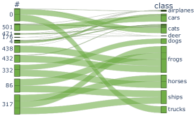
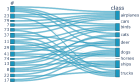
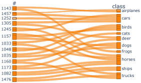
Figure 3: Application of Weighted-Filter layers for single-round multiple class unlearning on the CIFAR-10 dataset, using VGG-16 (left), ResNet-18 (middle), and ViT-S (right).

As it can be observed, WF-Net exhibits a proper unlearning behavior across all classes and models. In particular, we notice that on MNIST and CIFAR-10 it showcases a 0.0 accuracy on the forget sets when trained with VGG-16, ViT-S and ViT-T, underlying that the proposed strategy is effective in removing the knowledge of a class of choice, even without directly updating the model weights and while managing the unlearning of more classes concurrently. In terms of accuracy on the retain set, instead, we observe a restrained loss with respect to the performances of both the full model and of the retrained model. For example, on the ImageNet-1k dataset the CNN-based versions of WF-Net only lose a few accuracy points on the retain set compared to the accuracy of the original model (e.g., from 70.5 to 64.4 with ResNet-18). With Transformer-based architectures, instead, the loss in terms of retain accuracy is slightly more evident (e.g., from 82.3 to 69.2 with ViT-S).

When considering the ZRF score, computed on the unlearned classes, we can notice that the performance reached by our approach is always higher than that of the original model and generally in-line or higher than that of the retrained model, underlying again that our approach can properly unlearn. For completeness, we also report the activation distance and JS-divergence on MNIST and CIFAR-10, since both metrics require the retrained models to be computed. As it can be seen, both correlate with other scores.

Ablation study. We further assess the modeling choices behind WF-Net, by conducting an ablation study in which we compare against removing the reciprocal of the forget loss (i.e., using Eq. 2 instead of Eq. 3 as loss function, plus the regularizer), and when replacing the cross-entropy with an $\ell_{2}$ distance between the predicted logits and the logits of the original model. While the first ablation aims at validating the choice behind our final loss function, the second ablation study is motivated by the fact that output logits might carry more knowledge than labels, and might therefore be a good target for both retaining and unlearning the activations of the original network. Results are reported in Table 2 on the validation set of ImageNet-1k, and for all model architectures. We observe that the performance on both retaining and forgetting of WF-Net is superior to that exhibited by both the alternatives, highlighting the effectiveness of using the reciprocal of the forget loss, and that of using the cross-entropy with respect to ground-truth labels.

Unlearning without the training set. We then turn to the evaluation of a more complex setting, i.e. unlearning without having access to training data. Clearly, this is a more realistic scenario, as the training set might be inaccessible to the final user in several cases. Under this setting, the only option left would be to unlearn by collecting images which share approximately the same distribution of the training set. To simulate this setting, we unlearn over the 45k images of the validation set of ImageNet-1k not employed for evaluation, and evaluate over the usual evaluation set. From Table 3 we observe that the performance is reduced when unlearning without the training set, but our approach can still obtain sufficiently good performances, especially on ViT-S. Overall, this underlines that having access to the training set is still a requirement to have high-quality unlearning.

Insertion and deletion scores. In Table 4 we report the insertion and deletion scores, according to the four model architectures. The same scores are also visually depicted in Fig. 4 across different iterations. There, we compute both by considering the confidence score of the unlearned classes for images belonging to the unlearned classes (termed as “unlearned classes”) and for images belonging to other classes. As it can be seen, modifying the $\alpha$ values has an impact on the scores given to images belonging to unlearned classes, and not on images belonging to other classes. This highlights that the proposed approach can identify filters and attention weights which are responsible of the identification of each class.

Filter visualizations. Finally, in Fig. 3 we qualitatively visualize the association between filters (or attentive projections) and output classes, as discovered by the $\alpha$ values after unlearning, for randomly selected layers. To provide meaningful visualizations, we make use of the inverted version of $\alpha$ scores (i.e., $\bm{\hat{\alpha}}=1-\bm{\alpha}$). Following this, we select the top-10 filters for each class and remove the filters which do not appear in at least $r$ classes, in order to highlight filters which are shared between classes (with $r=2$ in Fig. 3). As it can be noticed, the proposed approach discovers proper relationships between filters and classes. For example, in the left visualization, we can notice how the filter #332 contributes to two different classes (i.e., dogs and horses), while in the middle graph the filter #3 contributes to the classes cats, deer, and dogs. These patterns can help to better understand the model behavior and can highlight the underlying relationships within the network.

		MNIST			CIFAR-10			ImageNet
		Insertion $\uparrow$	Deletion $\downarrow$		Insertion $\uparrow$	Deletion $\downarrow$		Insertion $\uparrow$	Deletion $\downarrow$
VGG-16		0.78	0.09		0.79	0.10		0.73	0.05
ResNet-18		0.79	0.05		0.69	0.06		0.75	0.04
ViT-T		0.90	0.07		0.88	0.05		0.60	0.04
ViT-S		0.90	0.08		0.88	0.14		0.75	0.04

Table 4: Insertion and deletion scores of the WF-Net model.

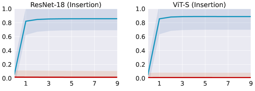
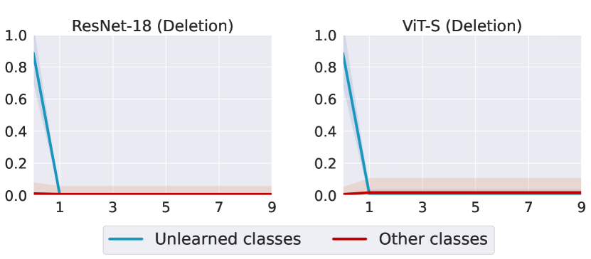
Figure 4: Insertion scores at different iterations for unlearned and retained classes.

5 Conclusion

We presented a novel approach for single-round multi-class unlearning. Given an image classification network, our approach can unlearn all classes simultaneously, in a single unlearning round. After training, the resulting network can be instructed to behave as if it has been untrained on any of the classes. Experimentally, we validated the effectiveness of the proposed framework on classical image datasets and across different architectures, also when unlearning without the training set. Our approach also discovers relationships between convolutional filters or attentive projections and output classes.

Appendix A Additional Implementation Details

Training details for original and retrained models. In our experiments, we consider the performance of original backbones, trained on the considered datasets. While for the ImageNet-1k dataset we directly employ the pre-trained models provided by the TorchVision and timm libraries (respectively for CNNs [35, 19] and ViT models [11]), we train from scratch all backbones on the training sets of MNIST and CIFAR-10. For these datasets, we also train the models without one of the available 10 classes (i.e. referred to “retrained models” in the main paper). During their training phase, we remove all samples of the left-out class from both the training and validation splits of the considered datasets. A good single-class unlearning process should aim to produce an unlearned model that behaves like these retrained models (i.e. their parameters should be drawn from the same distribution). In the main paper, we present a comparison between the retrained models and WF-Net, by averaging their overall performance.

To train the original and retrained models on MNIST and CIFAR-10, we use Adam [21] as optimizer, with a learning rate of $10^{-3}$ for the VGG-16 and ResNet-18 backbones, and $10^{-4}$ for both ViT-based models. We set a batch size of 256, and terminate training if the validation accuracy does not improve for 5 epochs. When training on the MNIST and CIFAR-10 datasets, we employ an image resolution equal to $32\times 32$, slightly upsampling images from the MNIST dataset. For the CIFAR-10 dataset, we also randomly apply random horizontal flip as data augmentation strategy. Furthermore, when training on the MNIST dataset, we adjust the input layer of all backbones, for compatibility with input gray-scale images.

WF-Net additional details. As mentioned in Section 4.3, the initialization of all the $\bm{\alpha}$ values to $3$ is necessary to guarantee that the initial performance is comparable to that of the original baseline model, and simultaneously prevents the sigmoid function from saturating. To sustain the assurance of this last eventuality, we clip all the $\bm{\alpha}$ parameters in $[-3,3]$ at every iteration.

(a) MNIST

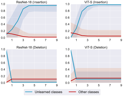
(b) CIFAR-10

Figure 5: Insertion scores at different iterations for unlearned and retained classes on MNIST (a) and CIFAR-10 (b).

Appendix B Insertion and Deletion Plots

The insertion and deletion plots depict the meaningfulness of the filters chosen by our WF-Net model. In particular, Figure 4 in the main paper and Figure 5 are generated calculating the insertion and deletion scores respectively on the ImageNet-1k (Figure 4), MNIST (Figure 5a), and CIFAR-10 (Figure 5b) datasets. For all the cases, we report the results on ResNet-18 and ViT-S backbones and also show the curve representing the values of the scores of the other classes, when the model sees images of the unlearned classes.

Insertion curve. It illustrates the rise of the model confidence score, as the most relevant $\bm{\alpha}$ values are re-activated. In all the datasets and models the insertion curve w.r.t. to the unlearned classes shows a steep growth, as expected, demonstrating the strong correlations between the lowest $\bm{\alpha}$ scores and the output classes. In contrast, since the model only sees images whose ground-truths are the unlearned labels, the curve corresponding to other classes does not benefit from the re-activation, as its scores remain close to $0$.

Deletion curve. As the counterpart of the insertion curve, it represents the drop of the model confidence score, as the most relevant $\bm{\alpha}$ values are deactivated. We start with the $\bm{\alpha}$ scores initialized to $3$ and then iteratively remove the most important filters. Again, in all the scenarios, it can be noticed how the score drops significantly at the very initial iterations. Conversely, the curve of other classes’ scores does not rise, meaning that those parameters are not significant if images whose ground-truths are the unlearned labels are input in the model. In fact, manipulating those particular $\bm{\alpha}$ values does not affect the performance of the model.

Appendix C Additional Filter Visualizations

In addition to the visualizations of the Weighted-Filter layers exhibited in the main paper, we report further qualitative illustrations for each backbone. Specifically, we show the associations between filters and output classes for different layers on both the MNIST and CIFAR-10 datasets, in Figure 6 and Figure 7 respectively.

As it can be noticed, the relationships between filters and classes are less evident in the first layers of the considered backbones. For instance, when examining ViT-S on the MNIST dataset, it can be observed that a single filter, like the filter #1072, contributes to a larger number of classes. However, as we move towards deeper layers, filters tend to specialize more on specific classes, and their corresponding $\bm{\alpha}$ values are usually lower. This is evident in the thicker associations seen in the parallel categories plots. In fact, in the final layer of ViT-S, the filters #1032 and #1038 are highly specialized towards two particular classes. These charts prove to be really useful for gaining insights into the internal functioning of a deep learning model since they present clear and unambiguous links from filters to output classes. This is one of the advantages given by our method.

Some of the highlighted relationships are directly evident: among the last-layer filters, the numbers #510 in VGG-16 and #17 in ResNet-18 for the CIFAR-10 dataset are specialized for classes that intuitively share common visual features, like dogs and cats. Other connections are less evident, at first sight, but it becomes clearer when we consider the nature of the images in the dataset. In fact, the filter #1160, in the selected intermediate layer in ViT-T, shows to be specialized for cats and horses, implying that those classes share some common characteristics.

Moreover, in the case of the filter #1033, ViT-S shows a link between cats and frogs, or between frogs and ships as in the filter #426 (intermediate layer). Some connections might be the result of the low-quality nature of the images in the CIFAR-10 dataset, given their $32\times 32$ resolution.

First Layer	Intermediate Layer	Last Layer

Figure 6: Application of Weighted-Filter layers for single-round multiple class unlearning on the MNIST dataset on different layers, using VGG-16 (first row), ResNet-18 (second row), ViT-T (third row), and ViT-S (fourth row).

First Layer	Intermediate Layer	Last Layer

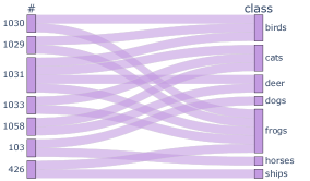
Figure 7: Application of Weighted-Filter layers for single-round multiple class unlearning on the CIFAR-10 dataset on different layers, using VGG-16 (first row), ResNet-18 (second row), ViT-T (third row), and ViT-S (fourth row).

References

- [1] Nasser Aldaghri, Hessam Mahdavifar, and Ahmad Beirami. Coded machine unlearning. IEEE Access, pages 88137–88150, 2021.
- [2] Thomas Baumhauer, Pascal Schöttle, and Matthias Zeppelzauer. Machine unlearning: Linear filtration for logit-based classifiers. Machine Learning, 111(9):3203–3226, 2022.
- [3] Alexander Binder, Grégoire Montavon, Sebastian Lapuschkin, Klaus-Robert Müller, and Wojciech Samek. Layer-wise relevance propagation for neural networks with local renormalization layers. In ICANN, 2016.
- [4] Lucas Bourtoule, Varun Chandrasekaran, Christopher A Choquette-Choo, Hengrui Jia, Adelin Travers, Baiwu Zhang, David Lie, and Nicolas Papernot. Machine unlearning. In IEEE Symposium on Security and Privacy, 2021.
- [5] Yinzhi Cao and Junfeng Yang. Towards Making Systems Forget with Machine Unlearning. In IEEE Symposium on Security and Privacy, 2015.
- [6] Aditya Chattopadhay, Anirban Sarkar, Prantik Howlader, and Vineeth N Balasubramanian. Grad-CAM++: Generalized Gradient-Based Visual Explanations for Deep Convolutional Networks. In WACV, 2018.
- [7] Vikram S Chundawat, Ayush K Tarun, Murari Mandal, and Mohan Kankanhalli. Can Bad Teaching Induce Forgetting? Unlearning in Deep Networks using an Incompetent Teacher. arXiv preprint arXiv:2205.08096, 2022.
- [8] Quang-Vinh Dang. Right to be forgotten in the age of machine learning. In International Conference on Advances in Digital Science, 2021.
- [9] Jia Deng, Wei Dong, Richard Socher, Li-Jia Li, Kai Li, and Li Fei-Fei. ImageNet: A large-scale hierarchical image database. In CVPR, 2009.
- [10] Jeff Donahue, Yangqing Jia, Oriol Vinyals, Judy Hoffman, Ning Zhang, Eric Tzeng, and Trevor Darrell. DeCAF: A Deep Convolutional Activation Feature for Generic Visual Recognition. In ICML, 2014.
- [11] Alexey Dosovitskiy, Lucas Beyer, Alexander Kolesnikov, Dirk Weissenborn, Xiaohua Zhai, Thomas Unterthiner, Mostafa Dehghani, Matthias Minderer, Georg Heigold, Sylvain Gelly, Jakob Uszkoreit, and Neil Houlsby. An Image is Worth 16x16 Words: Transformers for Image Recognition at Scale. In ICLR, 2021.
- [12] Shaopeng Fu, Fengxiang He, and Dacheng Tao. Knowledge removal in sampling-based bayesian inference. arXiv preprint arXiv:2203.12964, 2022.
- [13] Shaopeng Fu, Fengxiang He, Yue Xu, and Dacheng Tao. Bayesian inference forgetting. arXiv preprint arXiv:2101.06417, 2021.
- [14] Antonio Ginart, Melody Guan, Gregory Valiant, and James Y Zou. Making AI Forget You: Data Deletion in Machine Learning. In NeurIPS, 2019.
- [15] Aditya Golatkar, Alessandro Achille, Avinash Ravichandran, Marzia Polito, and Stefano Soatto. Mixed-privacy forgetting in deep networks. In CVPR, 2021.
- [16] Aditya Golatkar, Alessandro Achille, and Stefano Soatto. Eternal sunshine of the spotless net: Selective forgetting in deep networks. In CVPR, 2020.
- [17] Aditya Golatkar, Alessandro Achille, and Stefano Soatto. Forgetting outside the box: Scrubbing deep networks of information accessible from input-output observations. In ECCV, 2020.
- [18] Chuan Guo, Tom Goldstein, Awni Hannun, and Laurens Van Der Maaten. Certified data removal from machine learning models. arXiv preprint arXiv:1911.03030, 2019.
- [19] Kaiming He, Xiangyu Zhang, Shaoqing Ren, and Jian Sun. Deep Residual Learning for Image Recognition. In CVPR, 2016.
- [20] Zachary Izzo, Mary Anne Smart, Kamalika Chaudhuri, and James Zou. Approximate data deletion from machine learning models. In AISTATS, 2021.
- [21] Diederik P Kingma and Jimmy Ba. Adam: A Method for Stochastic Optimization. In ICLR, 2015.
- [22] Pang Wei Koh and Percy Liang. Understanding black-box predictions via influence functions. In ICML, 2017.
- [23] Alex Krizhevsky and Geoffrey Hinton. Learning multiple layers of features from tiny images. 2009.
- [24] Yann LeCun, Léon Bottou, Yoshua Bengio, and Patrick Haffner. Gradient-based learning applied to document recognition. Proceedings of the IEEE, 86(11):2278–2324, 1998.
- [25] Jianhua Lin. Divergence measures based on the Shannon entropy. IEEE Transactions on Information Theory, 37(1):145–151, 1991.
- [26] Scott M Lundberg and Su-In Lee. A unified approach to interpreting model predictions. In NeurIPS, 2017.
- [27] Emanuele Marconato, Andrea Passerini, and Stefano Teso. GlanceNets: Interpretabile, Leak-proof Concept-based Models. arXiv preprint arXiv:2205.15612, 2022.
- [28] Saumitra Mishra, Bob L Sturm, and Simon Dixon. Local interpretable model-agnostic explanations for music content analysis. In ISMIR, 2017.
- [29] Seth Neel, Aaron Roth, and Saeed Sharifi-Malvajerdi. Descent-to-delete: Gradient-based methods for machine unlearning. In International Conference on Algorithmic Learning Theory, 2021.
- [30] Quoc Phong Nguyen, Bryan Kian Hsiang Low, and Patrick Jaillet. Variational bayesian unlearning. In NeurIPS, 2020.
- [31] Thanh Tam Nguyen, Thanh Trung Huynh, Phi Le Nguyen, Alan Wee-Chung Liew, Hongzhi Yin, and Quoc Viet Hung Nguyen. A survey of machine unlearning. arXiv preprint arXiv:2209.02299, 2022.
- [32] Vitali Petsiuk, Abir Das, and Kate Saenko. RISE: Randomized Input Sampling for Explanation of Black-box Models. In BMVC, 2018.
- [33] Ramprasaath R Selvaraju, Michael Cogswell, Abhishek Das, Ramakrishna Vedantam, Devi Parikh, and Dhruv Batra. Grad-CAM: Visual Explanations From Deep Networks via Gradient-Based Localization. In ICCV, 2017.
- [34] Avanti Shrikumar, Peyton Greenside, and Anshul Kundaje. Learning important features through propagating activation differences. In ICML, 2017.
- [35] Karen Simonyan and Andrew Zisserman. Very Deep Convolutional Networks for Large-Scale Image Recognition. In ICLR, 2015.
- [36] Ayush K Tarun, Vikram S Chundawat, Murari Mandal, and Mohan Kankanhalli. Fast Yet Effective Machine Unlearning. arXiv preprint arXiv:2111.08947, 2021.
- [37] Andong Wang, Wei-Ning Lee, and Xiaojuan Qi. HINT: Hierarchical Neuron Concept Explainer. In CVPR, 2022.
- [38] Haofan Wang, Zifan Wang, Mengnan Du, Fan Yang, Zijian Zhang, Sirui Ding, Piotr Mardziel, and Xia Hu. Score-CAM: Score-weighted visual explanations for convolutional neural networks. In CVPR Workshops, 2020.
- [39] Alexander Warnecke, Lukas Pirch, Christian Wressnegger, and Konrad Rieck. Machine unlearning of features and labels. arXiv preprint arXiv:2108.11577, 2021.
- [40] Yinjun Wu, Edgar Dobriban, and Susan Davidson. Deltagrad: Rapid retraining of machine learning models. In ICML, 2020.
- [41] Matthew D Zeiler and Rob Fergus. Visualizing and understanding convolutional networks. In ECCV, 2014.