Black Box Few-Shot Adaptation for Vision-Language models

Abstract

Vision-Language (V-L) models trained with contrastive learning to align the visual and language modalities have been shown to be strong few-shot learners. Soft prompt learning is the method of choice for few-shot downstream adaptation aiming to bridge the modality gap caused by the distribution shift induced by the new domain. While parameter-efficient, prompt learning still requires access to the model weights and can be computationally infeasible for large models with billions of parameters. To address these shortcomings, in this work, we describe a black-box method for V-L few-shot adaptation that (a) operates on pre-computed image and text features and hence works without access to the model’s weights, (b) it is orders of magnitude faster at training time, (c) it is amenable to both supervised and unsupervised training, and (d) it can be even used to align image and text features computed from uni-modal models. To achieve this, we propose Linear Feature Alignment (LFA), a simple linear approach for V-L re-alignment in the target domain. LFA is initialized from a closed-form solution to a least-squares problem and then it is iteratively updated by minimizing a re-ranking loss. Despite its simplicity, our approach can even surpass soft-prompt learning methods as shown by extensive experiments on 11 image and 2 video datasets.
Code available at: https://github.com/saic-fi/LFA

1 Introduction

Large-scale Vision-Language (V-L) models [60] trained with contrastive learning currently represent the de-facto approach for few-shot visual adaptation. Their unprecedented success lies in part in the strength of the joint V-L embedding space learned by aligning the image and text modalities. However, when a V-L model is applied to a new domain, the domain shift exacerbates the V-L modality gap [48], and some sort of adaptation is required to obtain high accuracy (see Fig. 1(a)). The question that we want to address in this paper is: “can we effectively adapt a V-L model to a new domain by having access to pre-computed features only?” We call this black-box adaptation.

Similar to their NLP counterparts [60, 44], soft prompt learning has emerged as the preferred technique for adapting a V&L to new tasks. Specifically, a number of works [86, 85, 11, 87, 15, 67, 51, 36] have proposed to replace the manually designed prompts of [60] (e.g., a photo of a {cls_name}), with a sequence of learnable vectors, coined soft prompts. These are passed as input to the text encoder jointly with the class name cls_name to create the new prototypes effectively reducing the modality gap. The prompts are learned in a supervised manner using a standard cross-entropy loss given a set of labeled images.

While soft-prompt learning approaches demonstrate promising results on various downstream tasks [86, 85, 11], they suffer from two limitations: (1) They require access to the model’s weights, and (2) the training cost can be prohibitive, especially on commodity hardware and low-power devices, as computing the gradients and updating the prompts for thousands of iterations [86] is required. As the model’s size continues to grow (e.g., billion-parameter models such as CoCa [80]), and the industry transitions to models as a service (e.g., via API), the existing methods can be rendered either inapplicable or impractical.

Figure 1: Effect of Linear Feature Alignment (LFA): We use 16-shot (per class) training data for two fine-grained image classification datasets: DTD and FGVC Aircraft. In (1), we show the training set modality gap between paired image embeddings and class prototypes following the same procedure as in [48], and the obtained test set accuracy. The embeddings are visualized in 2D using PCA. (a) With CLIP features, we observe a big modality gap, resulting in low test accuracy. (b) After learning a set of soft-prompts, we obtain a better alignment and improved results. However, the modality gap is still not sufficiently reduced. (c) A simple linear transformation $\mathbf{W}$ that maps the original class prototypes (obtained using only the class names) to the ones obtained with soft-prompt learning induces a similar modality gap. (d) Motivated by (c) we propose LFA, which aligns the image embeddings with their class prototypes via linear mapping $\mathbf{W}$, obtained by solving a simple optimization problem. LFA results in better alignment and improved accuracy. In (2), we show that with LFA, the test image features are closely aligned with their corresponding class prototypes, resulting in higher cosine similarity scores compared to the ones obtained with soft prompts.

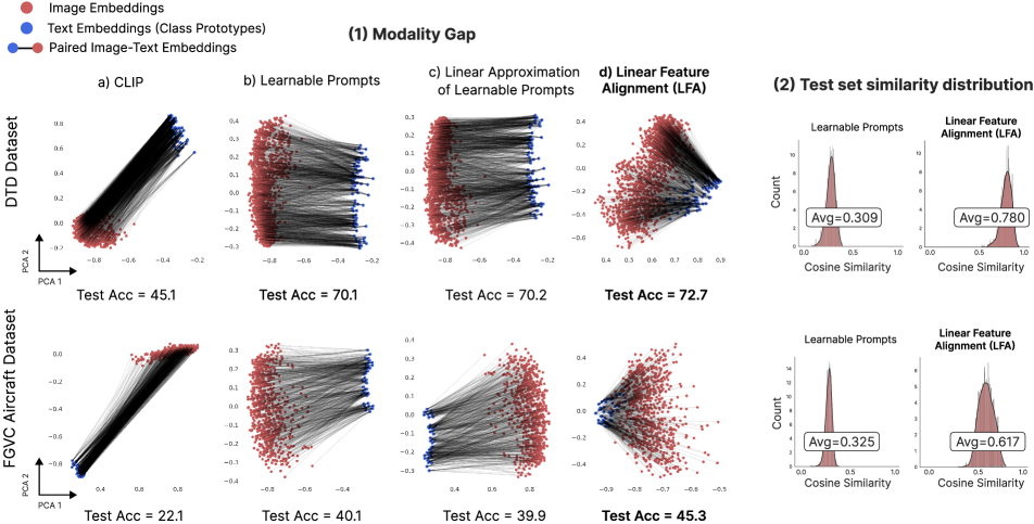
In this work, we seek to address these limitations by bridging the modality gap directly in the feature space without prompting or access to the model’s weights. We first empirically show that a simple linear transformation can approximate the alignment effect of prompt learning (e.g., see Fig. 1 and Sec. 3). Importantly, this shows that it is possible to derive a black-box method that manipulates the CLIP features directly for downstream adaptation. Then, motivated by this observation, we propose Linear Feature Alignment (LFA), a black-box method that learns a linear mapping $\mathbf{W}$, obtained by solving a simple optimization problem, which effectively aligns the image features $\mathbf{X}$ with their text class prototypes $\mathbf{Y}$, i.e., $\mathbf{X}\xrightarrow{\mathbf{W}}\mathbf{Y}$. Specifically, our contributions are:

• We propose the very first black-box method for the few-shot adaptation of V-L models.

• To this end, and motivated by the observation that prompting can be successfully approximated by a linear transformation, we propose Linear Feature Alignment (LFA), an efficient and effective adaptation method for reducing the modality gap between the image and text modalities of a V-L model. LFA is initialized by $\beta$-Procrustes, a regularized version of orthogonal Procrustes, and then minimizes a simple adaptive reranking loss adapted for V-L models.

• We propose both supervised and unsupervised formulations for LFA and moreover, a variant that works for the case of base-to-new (i.e., zero-shot) generalization.

• We demonstrate that LFA can achieve better alignment (e.g., see Fig. 1 (1d) and (2)) and improved accuracy compared to prompt learning methods while being more efficient (i.e., training takes few minutes) and practical (i.e., not requiring access to the model’s weights). Finally, we show that it can even align image and text features computed from uni-modal models.

Table 1: Training Time: train time for CoOp [86] and for the proposed LFA on ImageNet (16-shot) using ViT-B/16 as the visual encoder on a single V100 GPU.

Method	Training Time	Test Acc.
CoOp	3h 22min	71.92
LFA (Feature Extraction)	2min 37s
LFA (Procrustes Initialisation)	4s
LFA (Refinement)	28s
LFA (Total)	3min 9s	72.61

2 Related Work

Vision-Language (V-L) Models: Recently, we have witnessed an explosion of research in V-L foundation models, including CLIP [60], ALIGN [38], Florence [81], LiT [83], BASIC [59], ALBEF [46] and CoCa [80]. Such models are pre-trained on large amounts of image and text data to learn a joint multi-modal embedding space. After pre-training, they can be used on various downstream tasks in a few- or zero-shot setting. For our work, we used CLIP [60] to extract the frozen image and text features.

Learnable Prompts for V-L Models: Despite pre-training, V-L models still suffer from a modality gap [48] which is further exacerbated during downstream adaptation. To address this issue, recently, soft prompt learning methods [86, 85, 11, 87, 15, 67, 51, 36] optimize a new set of learnable (soft) prompts to reduce the gap and align the visual and text modalities. CoOp [86] was the first method to apply prompt learning methods [47, 44, 30, 66] popularized in NLP to V-L models. Subsequent works have improved upon this by incorporating image conditioning for better generalization [85], test-time adaptation [67], gradient matching [67], or by using an additional text-to-text loss [11]. In contrast to all the aforementioned methods, we propose to bridge the domain gap for a given downstream task directly in the feature space, without requiring access to the model’s weights nor expensive training procedures.

Linear Alignment: The problem of linearly aligning two sets of embeddings or high-dimensional real vectors is a well-studied problem in machine learning, with various applications in computer vision and NLP. Classical applications range from sentence classification [26, 62], to shape and motion extraction [72], registration [19] and geometrical alignment [24, 43, 49]. In vision, linear mappings are widely used for zero-shot learning [25, 1, 2, 64] for aligning the image features and their class attributes. In NLP, and after the introduction of word embeddings [53, 9], this linear alignment problem was revisited and extensively studied, and improved upon for the task of word translation [3, 27, 35, 18, 79, 54, 13, 39, 84, 68, 7, 6, 5, 4]. In this paper, we take strong inspiration from this line of work and set to adapt them for the case of V-L models.

3 Motivation: Approximating Soft Prompts with a Linear Transformation

Herein, we empirically show that the V-L alignment effect achieved by prompt learning can be approximated by finding a simple linear transformation $\mathbf{W}\in\mathbb{R}^{d\times d}$ that maps the class prototypes computed from the class names only (i.e., the class name text embeddings) to the ones obtained by soft prompt learning. To demonstrate this, let $\mathbf{Y}\in\mathbb{R}^{C\times d}$ be the class name embeddings represented in matrix form, and similarly, let $\mathbf{Y}^{\prime}\in\mathbb{R}^{C\times d}$ be the class prototypes obtained by soft prompt learning. Our objective is to learn a linear transformation $\mathbf{W}\in\mathbb{R}^{d\times d}$ that tries to approximate prompt learning, i.e., $\mathbf{Y}\xrightarrow{\mathbf{W}}\mathbf{Y}^{\prime}$, by solving the following least square problem:

$$\min_{\mathbf{W}\in\mathbb{R}^{d\times d}}\|\mathbf{Y}\mathbf{W}-\mathbf{Y}^{\prime}\|_{\mathrm{F}}^{2},$$ (1)

where $\|\cdot\|_{\mathrm{F}}$ is the Frobenius norm.

If the classification results are consistent when using either $\mathbf{Y}\mathbf{W}$ or $\mathbf{Y}^{\prime}$ as class prototypes, then we could use $\mathbf{Y}\mathbf{W}$ to approximate the V-L realignment achieved by prompt optimization. As shown in Fig. 1 (1b) and (1c), $\mathbf{W}$ can almost perfectly approximate the effects of prompt learning resulting in the same test set accuracy (i.e., same accuracy on DTD and 39.9 vs. 40.1 on FGVC Aircraft).

Note that, in practice, we want to avoid the training of the soft prompts. To this end, we can simply attempt to learn a linear transformation directly from the image features to the class name text embeddings. This is the main idea behind the proposed Linear Feature Alignment (LFA) which directly finds a linear transformation for image-text alignment.

4 Linear Feature Alignment

Our objective is to learn a linear mapping $\mathbf{W}$ for aligning the image embeddings $\mathbf{X}$ with their corresponding text class prototypes $\mathbf{Y}$, i.e., $\mathbf{X}\xrightarrow{\mathbf{W}}\mathbf{Y}$. Once $\mathbf{W}$ is learned, in order to classify a new sample $\mathbf{x}$, we obtain its $C$-way class probabilities from $\operatorname{softmax}(\mathbf{x}\mathbf{W}\cdot\mathbf{Y}^{\top}/\tau)$ with $\tau$ being the temperature parameter. To learn $\mathbf{W}$, LFA firstly uses for initialization a closed-form solution to a least-squares optimization problem, then minimizes a re-ranking loss to refine the initial solution. LFA is described in detail in the following sections.

4.1 Problem Formulation

Let $\mathbf{X}\in\mathbb{R}^{N\times d}$ be the image embeddings of $N$ examples produced by the CLIP image encoder, and let $\mathbf{Y}\in\mathbb{R}^{C\times d}$ be the $C$ class prototypes corresponding to the encoded class names using CLIP text encoder (i.e., without any prompts). Moreover, let $\mathbf{P}\in\mathcal{P}_{N\times C}$ be an assignment matrix that assigns each class prototype to its corresponding image embedding with $\mathcal{P}_{N\times C}=\{\mathbf{P}\in\{0,1\}^{N\times C},\ \mathbf{P}\mathbf{1}_{C}=\mathbf{1}_{N}\}$ as the set of binary permutation matrices that map each one of the $N$ rows to one of the $C$ columns, i.e., the input images to their corresponding classes. In a supervised setting where we are provided with $N$ (image-class) pairs, $\mathbf{P}$ is the stacked $N$ $C$-dimensional one-hot vectors.

Our objective is to find an optimal linear mapping that bridges the modality gap and aligns each image embedding with its text class prototype. To this end, the linear mapping can be learned by solving the following least squares:

$$\underset{\mathbf{W}\in\mathbb{R}^{d\times d}}{\operatorname{argmin}}\|\mathbf{X}\mathbf{W}-\mathbf{P}\mathbf{Y}\|_{\mathrm{F}}^{2}.$$ (2)

This is the standard Procrustes analysis formulation that aims to find a linear transformation between two sets of points $\mathbf{X}$ and $\mathbf{PY}$.

4.2 Orthogonal Procrustes

It is common to impose further constraints on the mapping $\mathbf{W}$ to adapt it to the task at hand. Of particular interest is the orthogonality constraint that has been shown empirically to be well-suited for mappings between different word embeddings and to result in improved alignment [79]. By enforcing the orthogonality constraint on $\mathbf{W}$, Eq. 2 becomes an Orthogonal Procrustes (OP) analysis optimization problem:

$$\mathbf{W}_{\mathrm{op}}=\underset{\mathbf{W}\in\mathcal{O}_{d}}{\operatorname{argmin}}\|\mathbf{X}\mathbf{W}-\mathbf{P}\mathbf{Y}\|_{\mathrm{F}}^{2},$$ (3)

with $\mathcal{O}_{d}=\{\mathbf{W}\in\mathbb{R}^{d\times d},\ \mathbf{W}^{\top}\mathbf{W}=\mathbf{I}_{d}\}$ as the set of orthogonal matrices and $\mathbf{I}_{d}$ as the $d$-dimensional identity matrix. As shown in [65], under this constraint, Eq. 3 admits a closed-form solution from the singular value decomposition (SVD) of $\mathbf{X}^{\top}\mathbf{P}\mathbf{Y}$:

$$\mathbf{W}_{\mathrm{op}} =\underset{\mathbf{W}\in\mathcal{O}_{d}}{\operatorname{argmin}}\|\mathbf{X}\mathbf{W}-\mathbf{P}\mathbf{Y}\|_{\mathrm{F}}^{2}=\mathbf{U}\mathbf{V}^{\top},$$ (4)

$$\text{with}\ \operatorname{SVD}(\mathbf{X}^{\top}\mathbf{P}\mathbf{Y})=\mathbf{U\Sigma}\mathbf{V}^{\top}.$$

Moreover, under the orthogonality constraint, the obtained mapping preserves the vector dot product and their $\ell_{2}$ distances, thus making it suitable for V-L models trained with a contrastive loss.

4.3 $\beta$-Procrustes

Figure 2: Effect of $\beta$-Procrustes: By pushing the orthogonal Procrustes solution of Eq. 4 towards an identity mapping via the update rule in Eq. 5, we avoid the overfitting exhibited using the original solution and obtain better alignment (i.e. as suggested by the observed class prototypes-image embeddings cross-interference). Here, each class prototype and its image embeddings share the same color and the embeddings shown are from 50 randomly sampled ImageNet classes.

Table 2: $\beta$-Procrustes: Top-1 acc. for 16-shot per class to obtain $\mathbf{W}$.

Method	ImageNet	Aircraft	DTD	Food101	Caltech101
CLIP ViT-B/16	62.8	22.1	45.1	83.9	88.0
Procrustes	52.5	27.9	63.4	78.8	93.4
$\beta$-Procrustes	64.8	29.1	65.8	85.5	94.7

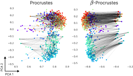
The orthogonal Procrustes solution is efficient and easy to compute, however, it suffers from extreme overfitting, especially if the initial modality gap is small. On ImageNet, for instance, and as shown in Fig. 2 and Tab. 2, the orthogonal Procrustes solution results in overly entangled class prototypes and a lower test accuracy than the original CLIP features (i.e., 62.8 $\rightarrow$ 52.5). To solve this, we propose $\beta$-Procrustes, a regularized Procrustes solution that is pushed to be close to an identity mapping via the following update:

$$\mathbf{W}_{\beta}\leftarrow\mathbf{W}_{\mathrm{op}}-\beta(\mathbf{W}_{\mathrm{op}}-\mathbf{I}_{d}),$$ (5)

where $\beta\in[0,1]$ is an interpolation hyperparameter between an identity mapping ($\beta=1$) and the orthogonal solution of Eq. 4 ($\beta=0$). This update is equivalent to a single gradient descent step of the regularization term $R_{\beta}(\mathbf{W}_{\mathrm{op}})=\frac{\beta}{2}\|\mathbf{W}_{\mathrm{op}}-\mathbf{I}_{d}\|_{\mathrm{F}}^{2}$, i.e. $\nabla_{\mathbf{W}_{\mathrm{op}}}R_{\beta}(\mathbf{W}_{\mathrm{op}})=\beta(\mathbf{W}_{\mathrm{op}}-\mathbf{I}_{d})$. As shown in Fig. 2 and Tab. 2, this simple update results in better alignment and improved test accuracy. For the choice of the hyperparameter $\beta$, it can be found via cross-validation on the training set or set to a fixed value with $\beta\in[0.6,0.9]$ without a significant impact on the results. The hyperparameter $\beta$ can be determined through cross-validation on the training set or set to a fixed value $\beta\in[0.6,0.9]$ without significantly impacting the results.

4.4 Mapping Refinement

Figure 3: Hubness: We show the rank of the ground-truth class prototypes of different training examples. We see that even after the $\beta$-Procrustes alignment step, the embedding space still contains a high number of hubs. After a refinement step, we reduce the hubness and obtain better image-class prototype alignment than soft-prompts.

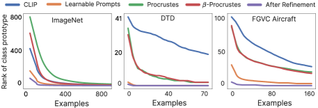
While $\beta$-Procrustes improves the results, they are still not on par with those obtained with the soft prompts. To investigate why, in Fig. 3, we show the rank of the ground-truth class prototype for different training examples, and we observe that even after the alignment with $\beta$-Procrustes, many examples have high ranks, i.e., they are closer to many other class prototypes than their own. At inference, this will result in many misclassifications. This is a known problem in many retrieval cases [8, 37], and is often caused by the hubness problem [61, 22, 18, 39]. Hubs are points (e.g., class prototypes) in the high dimensional vector space that are the nearest neighbors of many other points (e.g., image embeddings), and as a result, they greatly influence the classification probabilities (and thus the accuracy at test time).

To mitigate this effect, and inspired by popular metric learning losses [29, 70, 75, 76, 12], we propose to refine the mapping $\mathbf{W}$ by optimizing an Adaptive Reranking (ARerank) loss designed specifically to reduce the hubness problem, and defined as follows:

$$\mathcal{L}_{\mathrm{ARerank}}(\mathbf{x}_{i}\mathbf{W},\mathbf{Y}) =\frac{1}{k}\sum_{\mathbf{y}_{j}\in\mathcal{N}_{k}(\mathbf{x}_{i}\mathbf{W})}\ell_{ij}$$ (6)

$$\text{where}\ \ \ell_{ij} =\max\{d_{ii}-d_{ij}+m_{ij},0\},$$

where $d_{ii}=\|\mathbf{x}_{i}\mathbf{W}-\mathbf{y}_{c_{i}}\|_{2}$ is the $\ell_{2}$ distance between the aligned image embedding $\mathbf{x}_{i}\mathbf{W}$ and its class prototype $\mathbf{y}_{c_{i}}$, and similarly, $d_{ij}=\|\mathbf{x}_{i}\mathbf{W}-\mathbf{y}_{j}\|_{2}$ the $\ell_{2}$ distance between the aligned image embedding and each of its $k$ nearest class prototypes $\mathbf{y}_{j}\in\mathcal{N}_{k}(\mathbf{x}_{i}\mathbf{W})$, and $m_{ij}$ the margin. Empirically, we found that $k=3$ works well for most datasets.

To make the re-ranking dynamic and avoid having multiple hyperparameters, we opt for an adaptive margin selection approach similar to [45]. Specifically, the margin between image $i$ and a given class prototype $j$ is defined based on the cosine similarity between its class prototype $\mathbf{y}_{c_{i}}$ and the $j$-th class prototype, i.e., $m_{ij}=(1.0-\mathbf{y}_{c_{i}}^{\top}\mathbf{y}_{j})/s$, where $s$ is a scalar set to 4 for all experiments. By doing so, we ensure that each image embedding is pushed away from nearby incorrect class prototypes with an adaptive margin, while the distance to its class prototype is kept unchanged, thus mitigating the hubness problem and avoiding learning a degenerate mapping. As shown in Tab. 3, ARerank loss outperforms standard embedding optimization losses, and also demonstrates better results than the CSLS criterion proposed by [18] used to reduce hubness for word translation. Finally, as shown in Tab. 4, the coupling of $\beta$-Procrustes and ARerank-based refinement results in better accuracy.

Table 3: Refinement Loss: Top-1 acc. for 16-shot per class.

Refinement Loss	ImageNet	Aircraft	DTD	Food101	Caltech101
CLIP ViT-B/16	62.8	22.1	45.1	83.9	88.0
$\beta$-Procrustes	64.8	29.1	65.8	85.5	94.7
Contrastive	65.5	40.1	71.5	85.7	92.2
Triplet with margin	70.7	43.5	72.6	86.9	95.9
CSLS	71.1	40.9	72.2	86.8	95.9
ARerank	71.7	45.1	72.7	87.5	95.9

Table 4: $\beta$-Procrustes & Mapping Refinement: Top-1 acc. for 16-shot per class.

Method	ImageNet	Aircraft	DTD	Food101	Caltech101
CLIP $\rightarrow$ Refine	71.6	43.4	72.6	87.2	95.9
CLIP $\rightarrow$ Proc. $\rightarrow$ Refine	70.7	44.8	72.4	85.3	95.7
CLIP $\rightarrow$ $\beta$-Proc. $\rightarrow$ Refine	71.7	45.1	72.7	87.5	95.9

Algorithm 1 Linear Feature Alignment (LFA)

⬇

def LFA(img_feats, cls_prototypes, labels, beta, test_img_features):

"""

␣␣␣␣img_feats:␣[N,␣d]

␣␣␣␣cls_prototypes:␣[C,␣d]

␣␣␣␣labels:␣[N]

␣␣␣␣test_img_features:␣[M,␣d]

␣␣␣␣#␣N:␣number␣of␣training␣image␣features

␣␣␣␣#␣C:␣number␣of␣classes

␣␣␣␣#␣d:␣features␣dimensionality

␣␣␣␣#␣M:␣number␣of␣test␣image␣features

␣␣␣␣"""

# One-to-one matchings

text_feats = cls_prototypes[labels]

# Orthogonal Procrustes

u, _, v = torch.svd(img_feats.T @ text_feats)

W_op = u @ v.T

# Beta-Procrustes

identity = torch.eye(d)

W_beta = W_op - (W_op - identity) * beta

# Refine

W = adaptive_rerank_refine(W_beta)

test_logits = (test_img_features @ W) @ cls_prototypes.T

test_preds = test_logits.argmax(-1)

return test_preds

4.5 Overall LFA algorithm

Herein, we define the overall algorithm obtained by combining the steps defined in the previous sections. We consider two cases: supervised learning, where labeled data is provided, and unsupervised learning, where only unlabeled images are available.

Supervised Alignment: In a supervised setting, we can directly construct the assignment matrix $\mathbf{P}$ between the image embeddings $\mathbf{X}$ and class prototypes $\mathbf{Y}$ using the ground-truth data. The overall algorithm can be then defined as (see also Alg. 1):

1. $\mathbf{W}_{\mathrm{op}}\leftarrow$ Orthogonal Procrustes [$\mathbf{X},\mathbf{P}\mathbf{Y}$] (Eq. 4).

2. $\mathbf{W}_{\beta}\leftarrow$ $\beta$-Procrustes[$\mathbf{W}_{\mathrm{op}}$] (Eq. 5).

3. $\mathbf{W}\leftarrow$ Refine [$\mathbf{W}_{\beta}$, $\mathbf{X},\mathbf{P}\mathbf{Y}$] (Eq. 6).

Unsupervised Alignment: In an unsupervised setting, the correspondences between the image embeddings and their class prototypes are not known a priori. Thus the assignment matrix $\mathbf{P}$ must be estimated jointly with learning the mapping $\mathbf{W}$. By keeping the orthogonality constraint over $\mathbf{W}$ and solving for both $\mathbf{P}$ and $\mathbf{W}$, the resulting optimization problem, often referred to as the Wasserstein-Procrustes [84, 27] problem takes the following form:

$$\mathbf{W}^{\star},\mathbf{P}^{\star}=\underset{\mathbf{W}\in\mathcal{O}_{d},\mathbf{P}\in\mathcal{P}_{N\times C}}{\operatorname{argmin}}\|\mathbf{X}\mathbf{W}-\mathbf{P}\mathbf{Y}\|_{\mathrm{F}}^{2}.$$ (7)

As neither of the two sets $\mathcal{O}_{d}$ and $\mathcal{P}_{N\times C}$ are convex, this optimization problem is not convex either. To solve it, in practice, we follow a simple heuristic by alternating between finding the assignments $\mathbf{P}$ using the efficient Sinkhorn algorithm [20] and refining the mapping following Eq. 6. Given this, Unsupervised LFA (U-LFA) takes the following form:

1. $\mathbf{P}\leftarrow$ Sinkhorn [$\mathbf{X},\mathbf{Y}$].

2. $\mathbf{W}_{\mathrm{op}}\leftarrow$ Orthogonal Procrustes [$\mathbf{X},\mathbf{P}\mathbf{Y}$].

3. $\mathbf{W}\leftarrow$ $\beta$-Procrustes[$\mathbf{W}_{\mathrm{op}}$].

4. Repeat for $n$ iterations:

   1. $\mathbf{P}\leftarrow$ Sinkhorn [$\mathbf{X}\mathbf{W},\mathbf{Y}$].

   2. $\mathbf{W}\leftarrow$ Refine [$\mathbf{W}$, $\mathbf{X},\mathbf{P}\mathbf{Y}$].

Table 5: U-LFA: Top-1 acc. for 16-shot per class (without labels):

Refinement Loss	ImageNet	Aircraft	DTD	Food101	Caltech101
CLIP ViT-B/16	62.8	22.1	45.1	83.9	88.0
U-LFA ($n=1$)	66.9	24.5	48.0	86.7	94.4
U-LFA ($n=5$)	68.6	24.2	47.5	86.1	95.1
with template: a photo of a {cls name}.
CLIP ViT-B/16	66.8	23.3	43.9	85.8	92.9
U-LFA ($n=1$)	69.1	27.9	50.2	87.4	95.3
U-LFA ($n=5$)	70.3	28.0	49.0	86.6	95.5

Table 6: LFA analysis under distribution shift: Top-1 acc. for 16 shots per class on the Base (B) and New (N) sets and two IN variants. IN refers to ImageNet.

Method	Language Shift							Image Shift
	ImageNet		Aircraft		DTD
	B	N	B	N	B	N		IN-A	IN-R
LFA	76.9	67.1	41.5	30.7	81.6	54.9		49.7	74.5
LFA (average)	76.8	68.6	40.7	31.8	81.6	59.7		50.6	75.5
LFA (two mappings)	76.9	69.4	41.5	32.3	81.6	60.6		51.5	76.1

4.6 LFA for Base-to-New (Zero-Shot) Recognition

Table 7: Augmentations: average Top-1 acc. for 16-shot per class on 11 datasets using 5 crops per image, with and without a prompt template.

Backbone	RN50	RN101	ViT-B/32	ViT-B/16
LFA	74.20	76.83	76.69	80.54
LFA + 5 crops	74.49	77.05	76.95	80.88
LFA + 5 crops + template	74.75	77.14	77.17	81.21

Table 8: Few-shot Classification: Top-1 acc. for 16-shot per class when using CLIP, CoOp [86] and LFA, with either RN50, RN101, ViT-B/32 or ViT-B/16 as the vision encoder.

Method	Pets	Flowers102	Aircraft	DTD	EuroSAT	Cars	Food101	SUN397	Caltech101	UCF101	ImageNet	Avg.	$\Delta$
CLIP RN50	85.77	66.14	17.28	42.32	37.56	55.61	77.31	58.52	86.29	61.46	58.18	58.77
CoOp	86.16	94.80	32.29	63.16	83.55	73.27	74.46	69.12	91.62	75.29	63.08	73.35
LFA	86.75	94.56	35.86	66.35	84.13	73.58	76.32	71.32	92.68	77.00	63.65	74.75	+1.40
CLIP RN101	86.75	64.03	18.42	38.59	32.59	66.23	80.53	58.96	89.78	60.96	61.62	59.86
CoOp	88.57	95.19	34.76	65.47	83.54	79.74	79.08	71.19	93.42	77.95	66.60	75.96
LFA	88.80	93.11	39.62	68.95	83.43	79.45	81.57	72.69	94.53	79.28	67.16	77.14	+1.18
CLIP ViT-B/32	87.49	66.95	19.23	43.97	45.19	60.55	80.50	61.91	90.87	62.01	62.05	61.88
CoOp	88.68	94.97	33.22	65.37	83.43	76.08	78.45	72.38	94.62	78.66	66.85	75.70
LFA	88.62	93.84	38.01	68.87	83.88	76.72	81.31	74.12	95.10	80.81	67.63	77.17	+1.47
CLIP ViT-B/16	89.21	71.34	24.72	44.39	47.60	65.32	86.06	62.50	92.94	66.75	66.73	65.23
CoOp	92.53	96.47	42.91	68.50	80.87	83.09	87.21	75.29	95.77	82.24	71.92	79.71
LFA	92.41	96.82	46.01	71.89	87.31	82.23	87.14	76.65	96.24	83.99	72.61	81.21	+1.50

Table 9: Out-of-Domain Generalization: the obtained average Top-1 acc. on various ImageNet variants after training on ImageNet (i.e., source) using 16-shot training data per class and using RN50 as the visual encoder. We show the results for the baseline CLIP [60], CoOp [86], CoCoOp [85], and the proposed LFA on each dataset, their average and the Out-of-Distribution (OOD) average (i.e., over the target datasets).

	Source		Target
Method	ImageNet		ImageNet-A	ImageNet-V2.	ImageNet-R.	ImageNet-Sketch	Avg.	OOD Avg.	$\Delta$
CLIP-RN50	58.16		21.83	51.41	56.15	33.37	44.18	40.69
CoOp	63.33		23.06	55.40	56.60	34.67	46.61	42.43
CoCoOp	62.81		23.32	55.72	57.74	34.48	46.81	42.82
LFA	63.88		24.31	55.79	58.13	34.37	47.29	43.15	+0.32
CLIP-ViT-B/16	66.73		47.87	60.86	73.98	46.09	59.11	57.2
CoOp	71.51		49.71	64.20	75.21	47.99	61.72	59.28
CoCoOp	71.02		50.63	64.07	76.18	48.75	62.13	59.91
LFA	72.65		51.50	64.72	76.09	48.01	62.59	60.08	+0.17

Table 10: Few-shot Action Recognition: Top-1 acc. for 8 and 16-shot per class. We compare against our implementation of Video Prompting [40], which is trained either with mean over the per-frame features (i.e., Temporal: ✗) or a single Transformer layer (i.e., Temporal: ✓).

N-shot	Method	Soft-Prompt	Temporal	UCF-101	HMDB51	Avg.	$\Delta$
	CLIP [60, 40]	hand-craft	✗	64.7	40.1	52.40
8	Video Prompting	✓	✗	73.37	49.72	61.54
	Video Prompting	✓	✓	86.21	60.52	73.36
	LFA	✗	✗	87.60	60.74	74.17	+0.81
16	Video Prompting	✓	✗	76.22	53.90	65.06
	Video Prompting	✓	✓	89.43	65.05	77.24
	LFA	✗	✗	89.47	65.08	77.27	+0.03

Table 11: Action Recognition: the obtained Top-1 acc. on the test sets of UCF101 and HMDB51 using the full training sets. Video Prompting [40] is trained with two Transformer layers (i.e., Temporal: ✓) on top of the frozen per-frame CLIP features to model the temporal information in the input video segment. All results are obtained with ViT-B/16 as the visual encoder.

Method	Soft-Prompt	Temporal	UCF-101	HMDB51	Avg.	$\Delta$
I3D [14]			74.3	95.1	84.7
S3D-G [78]			75.9	96.8	86.3
R(2+1)D [73]			74.5	96.8	85.6
R3D-50 [31]			66.0	92.0	79.0
Video Prompting	✓	✓	66.4	93.6	80.0
LFA	✗	✗	69.2	91.8	80.5	+0.5

An important property of large-scale V-L models that recent few-shot adaptation methods seek to preserve is their zero-shot generalization ability, i.e., generalization from seen (base) classes to unseen (new) classes. Training LFA in this setting, i.e., on the base set, may result in a mapping that fails to generalise to the new set due to the distribution shift in between the two.

To address this, starting from a task-specific mapping $\mathbf{W}$, during the iterative refinement step, we initialize a second $\mathbf{W}_{\mathrm{tt}}$ as an identity map $\mathbf{I}_{d}$. At each optimization step $t$ of the refinement procedure, we then update $\mathbf{W}_{\mathrm{tt}}$ using $\mathbf{W}$ with an exponential moving average as follows:

$$\mathbf{W}_{\mathrm{tt}}(t)\leftarrow\alpha(t)\mathbf{W}_{\mathrm{tt}}(t)+(1-\alpha(t))\mathbf{W}(t)$$ (8)

with $\alpha(t)\in[0,1]$ as the momentum parameter, which is initialized as 0.9, and is increased to 1.0 following a log schedule during the first half of the optimization. This way, we only incorporate the first refinement updates into $\mathbf{W}_{\mathrm{tt}}$, while the later ones, which tend to be more task-specific and may hinder generalization are largely ignored. At test time, $\mathbf{W}$ can be used on the base classes, while $\mathbf{W}_{\mathrm{tt}}$ for the new classes. As shown in Tab. 6, this maintains the good accuracy on the base training domain, while demonstrating good generalization when a distribution shift occurs (i.e., on novel classes). Additionally, using a single mapping, obtained by taking the average of $\mathbf{W}$ and $\mathbf{W}_{\mathrm{tt}}$ also achieves good results (see Tab. 6).

5 Experiments

Datasets & Evaluation settings: For image classification, we consider the following evaluation protocols and settings: (1) standard few-shot classification, as in [86], (2) generalisation from base-to-new classes, where the model is trained in a few-shot manner on the base classes and tested on a disjoint set of new classes, as in [85], and finally, (3) domain generalisation, where the model is trained on training set of ImageNet and is then tested on one of the four ImageNet variants with some form of distribution shift, as in [85, 86]. For standard few-shot evaluation and generalisation from base-to-new classes, we report results on the 11 datasets used in CoOp [86]: ImageNet [21], Caltech101 [23], OxfordPets [57], StanfordCars [41], Flowers102 [56], Food101 [10], FGVCAircraft [52], SUN397 [77], UCF101 [69], DTD [17] and EuroSAT [32]. For domain generalisation, we follow previous work [86, 85] and report the classification results on four ImageNet variants: ImageNetV2 [63], ImageNet-Sketch [74], ImageNet-A [34] and ImageNet-R [33].

For action recognition, we align our setting with [40] and consider both standard (i.e. using the full training set for adaptation) and few-shot classification settings and on two datasets, HMDB51 [42] and UCF101 [69]. To get the video features to be aligned their class prototypes, we take the max aggregate on the per-frame CLIP features.

Implementation Details: Unless stated otherwise, we base our experiments on a pre-trained CLIP model [60]. For each experiment, we pre-compute and save the image features alongside the class prototypes and follow the adaptation procedure as described in Section 4.5. The class prototypes are formed by inserting the class name in the standard templates [86] (e.g., “a photo of a {cls name}” for image tasks and “a video frame of a person {action type}” for videos). As it is common practice to augment the images for prompting [85, 86], for each training image, we construct $c=5$ random cropped views, noting that a large $c$ is not crucial, as LFA still performs well without them (i.e., $c=1$), as shown in Tab. 7.

Training Details: For standard image few-shot experiments, we set $\beta$ based on cross-validation on the training set, while for the rest, we fix it to $\beta=0.9$. For the refinement step, we set $k=3$ for the ARerank loss, and finetune the mappings using AdamW [50] for 50-200 iterations using a learning rate of 5e-4, a weight decay of 5e-4, and a cosine scheduler. During refinement, we inject a small amount of Gaussian noise (i.e., std of 3.5e-2) and apply dropout (i.e., 2.5e-2) to the image embeddings to stabilize training. For few-shot experiments, we follow standard practices and report the average Top-1 accuracy over 3 runs. For additional details, refer the supplementary material.

5.1 Comparisons with State-of-the-Art

Standard Few-shot Image Classification: As show in Tab. 8, LFA outperforms CoOp [86] by 1% on average over the 11 datasets and with various visual backbones, with the biggest gains observed on datasets with larger domain gaps, i.e., $\approx 7\%$ on EuroSAT.

Base-to-New Generalisation: Using 2 mappings, and as shown in Tab. 12, LFA improves the prior best result of ProDA by $2.18\%$ in terms of harmonic mean, with similar improvements for both base and new classes. Again, the largest gains are observed for datasets with larger domain gaps, such as UCF101 and EuroSAT.

Table 12: Base-to-New generalization: Top-1 acc. for 16-shot per base class.

Dataset	Set	CLIP	CoOp	CoCoOp	ProDA	LFA	$\Delta$
ImageNet	Base	72.43	76.47	75.98	75.40	76.89
	New	68.14	67.88	70.43	70.23	69.36
	H	70.22	71.92	73.10	72.72	72.93	-0.17
Caltech101	Base	96.84	98.0	97.96	98.27	98.41
	New	94.00	89.91	93.81	93.23	93.93
	H	95.40	93.73	95.84	95.86	96.13	+0.27
Pets	Base	91.17	93.67	95.20	95.43	95.13
	New	97.26	95.29	97.69	97.83	96.23
	H	94.12	94.47	96.43	96.62	95.68	-0.94
Cars	Base	63.37	78.12	70.49	74.70	76.32
	New	74.89	60.40	73.59	71.20	74.88
	H	68.85	68.13	72.01	72.91	75.59	+2.68
Flowers102	Base	72.08	97.60	94.87	97.70	97.34
	New	77.80	59.67	71.75	68.68	75.44
	H	74.83	74.06	81.71	80.66	85.00	+3.29
Food101	Base	90.10	88.33	90.70	90.30	90.52
	New	91.22	82.26	91.29	88.57	91.48
	H	90.66	85.19	90.99	89.43	91.00	+0.0
Aircraft	Base	27.19	40.44	33.41	36.90	41.48
	New	36.29	22.3	23.71	34.13	32.29
	H	31.09	28.75	27.74	35.46	36.31	+0.85
SUN397	Base	69.36	80.6	79.74	78.67	82.13
	New	75.35	65.89	76.86	76.93	77.20
	H	72.23	72.51	78.27	77.79	79.59	+1.78
DTD	Base	53.24	79.44	77.01	80.67	81.29
	New	59.9	41.18	56.0	56.48	60.63
	H	56.37	54.24	64.85	66.44	69.46	+3.02
EuroSAT	Base	56.48	92.19	87.49	83.90	93.40
	New	64.05	54.74	60.04	66.0	71.24
	H	60.03	68.9	71.21	73.88	80.83	+6.95
UCF101	Base	70.53	84.69	82.33	85.23	86.97
	New	77.50	56.05	73.45	71.97	77.48
	H	73.85	67.46	77.64	78.04	81.95	+3.90
Average	Base	69.34	82.69	80.47	81.56	83.62
	New	74.22	63.22	71.69	72.30	74.56
	H	71.70	71.66	75.83	76.65	78.83	+2.18

Domain Generalisation: As in base-to-new generalisation, we report the results obtained with two mappings as detailed in Section 4.6. As shown in Tab. 9, LFA outperforms CoOp [86] on the source domain, while also outperforming CoCoOp [85] on the target domains, These results further demonstrate the flexibility of LFA, which can be used to adapt to different domains and settings, and even under a test-time distribution shift, either on the language or the image side.

Standard Action Recognition: Tab. 11 shows the obtained action recognition results when using the full-training set for video-text alignment. LFA slightly outperforms the video soft-prompting method of [40] on average, and by a notable margin on HMDB51. However, and different from [40] that trains two transformer layers on top of the frozen per-frame CLIP features to model the temporal information in addition to the soft-prompt, LFA matches performances of [40] without any temporal modeling.

Few-shot Action Recognition: similar to the standard setup, and as shown in Tab. 10, LFA largely matches or outperforms the performances of [40] with no temporal modeling.

Table 13: Aligning Disjoint Modalities for Few-shot Classification: Top-1 acc. for 16-shot per class after aligning the visual and language features of separate (i.e. uni-modal) vision and language encoders. We use 3 self-supervised RN50 vision encoders and the OpenAI embeddings API to access the cpt-text encoder [55] and generate the class prototypes. kNN classifier and linear probe results are obtained by training on the visual features.

Visual Enc.	Text Enc.	Method	Pets	Flowers102	Aircraft	DTD	EuroSAT	Cars	Food101	SUN397	Caltech101	UCF101	ImageNet	Avg.	$\Delta$
BYOL [28]	OpenAI Emb.	kNN	69.24	75.84	11.63	54.77	80.58	10.88	30.13	42.04	85.89	51.12	44.57	50.61
		Linear Probe	76.08	82.70	13.80	62.07	87.06	14.87	37.01	47.50	90.04	59.59	48.91	56.33
		LFA	79.84	92.81	32.03	63.83	88.82	36.98	45.78	53.72	92.2	66.82	54.04	64.26	+7.93
BarlowTwins [82]	OpenAI Emb.	kNN	68.73	79.87	14.79	54.73	81.66	12.01	30.71	41.35	84.07	49.07	41.44	50.77
		Linear Probe	75.78	85.14	16.92	62.53	87.92	15.89	37.4	45.94	88.93	56.6	45.01	56.19
		LFA	79.39	93.24	35.02	63.71	89.65	41.29	46.02	52.66	91.70	64.95	51.34	64.45	+8.26
MoCo v3 [16]	OpenAI Emb.	kNN	78.13	80.63	18.66	54.39	81.74	14.56	32.10	44.23	91.13	55.36	50.10	54.64
		Linear Probe	83.81	86.97	20.59	61.94	88.61	18.83	39.47	49.24	93.52	63.34	53.55	59.99
		LFA	85.18	93.36	39.75	62.71	89.13	45.36	46.15	54.22	94.25	68.21	57.57	66.90	+6.91

5.2 Ablation studies

In this section, we (1) ablate the impact of the proposed closed-form relaxed initialisation, (2) compare the new re-ranking loss with a series of baselines, and (3) analyse the effect of the number of image crops and of template-based text prompting for class prototyping. Moreover, to showcase the generalisability of our approach, (4) we explore our method’s behaviour on disjoint models, where the vision and text encoder are trained from separate sources, (5) the effectiveness of LFA with V-L models other than CLIP, (6) the results sensitivity to the choice of $\beta$. Finally, (7) we report results for the unsupervised variant of our method. See supplementary material for some additional ablations.

Effect of closed-form initialisation and refinement: The proposed $\beta$-Procrustes regularization significantly reduces overfitting (Tab. 2) and provides a notably better starting point for the refinement process (Tab. 4) across all datasets.

ARerank vs other losses: In Tab. 3 we compare the proposed ARerank loss with a series of baselines, out of with the CSLS loss is the closest conceptually to ours. As the results show, we outperform CSLS across all datasets by up to $4\%$. Moreover, we improve between 1.6% (for Imagenet) and $5\%$ (for FGVC) on top of the standard contrastive loss.

Effect of the number of image crops and prototype templating: As show in Tab. 7, LFA is largely invariant to the exact number of crops per image used for training, showing strong results with a single crop (Tab. 7). Additionally, and similar to [11, 85], the results show that the usage of prompting templates for constructing the class prototypes to be beneficial.

Table 14: LFA and Soft-Prompts: Top-1 acc. on ImageNet for 16-shot per class when using trained soft-prompts (e.g., CoOp [86]) to generate the class prototypes.

Backbone	RN50	RN101	ViT-B/32	ViT-B/16
CoOp	62.62	66.45	66.41	71.62
LFA	63.65	67.16	67.63	72.61
LFA + CoOp	63.78	67.72	67.85	73.10

LFA and soft-prompts: To further show the complementarity and flexibility of LFA, we use a set of pre-trained soft-prompts (i.e., CoOp [86]) to obtain the class prototypes. Then we proceed with the LFA procedure. As shown in Tab. 14, LFA can also be coupled with soft-prompts for additional improvements.

Other V-L models: Given the black-box nature of LFA, it can be used as is with other V-L models and with similar gains in performance as CLIP. Tab. 15 shows the results obtained with LFA when using other V-L models further confirming the generality and flexibility of LFA.

Table 15: LFA with various V-L models: Top-1 acc. on ImageNet for 16-shot per class when using features from V-L models other than CLIP.

Method	ALIGN [38]	FLAVA [38]	AltCLIP [38]
Zero-shot	64.4	54.6	73.5
LFA (ImageNet 16-shot)	69.8 (+5.4)	61.1 (+6.5)	79.1 (+5.6)

Sensitivity to the choice of $\beta$: While it is beneficial to tune $\beta$ for each dataset using cross-validation, Tab. 16 shows that the final results remain robust to the choice of $\beta$, and setting $\beta\in[0.6,0.9]$ results in similar performances.

Table 16: Sensitivity to $\beta$: Top-1 acc. on ImageNet for 16-shot per class with different $\beta$ values.

$\beta$	0.0	0.1	0.2	0.3	0.4	0.5	0.6	0.7	0.8	0.9
LFA	71.04	71.39	71.67	71.87	72.08	72.26	72.45	72.54	72.56	72.54

Performance analysis for disjoint modalities: Our approach is modality, domain, and architecture agnostic. Moreover, it doesn’t require access to the weights, only to the produced features. To showcase this, we introduce a new evaluation setting in which the visual and text features are produced by disjoint models, that never interacted during training. Either one or both modalities can be sourced from behind-the-wall (i.e., blackbox) models. For this experiment, we consider 3 RN50 pre-trained visual backbones: BYOL, BarlowTwins and MoCo v3. As we do not require access to the model, we use the OpenAI embeddings API to get the text embeddings from the cpt-text encoder [55] and generate the class prototypes. After an initial random projection to project the image features into the 1536-d space and match the dimensionality of text features, we proceed with the supervised LFA procedure as with CLIP experiments. In a few-shot setting, alongside our method, we consider 2 baselines that also operate the frozen visual features: kNN and linear eval (see supplementary material for the hyper-parameters used). As the results from Tab. 13 show, our method (1) reaches performance comparable with that of aligned models (i.e., CLIP) and (2) outperforms both kNN and linear eval by a large margin.

Unsupervised LFA: As presented in Section 4.5, LFA can be adapted for label-free training. Tab. 5 shows that U-LFA improves by up to 7% on top of zero-shot CLIP.

6 Conclusions

In this work we proposed LFA, the first black box few-shot adaptation method for V-L models, that uses pre-computed image and text features without accessing the model’s weights. Other advantages of LFA include fast training, applicability to both supervised and unsupervised setting, and even application for aligning image and text features computed from uni-modal models. Thanks to the use of precomputed features, we hope that LFA will enable few-shot adaptation of very large V-L foundation models that would otherwise be impossible to adapt or even deploy.

Appendix A Appendix

Table 17: Few-shot Classification: the obtained average Top-1 test acc. on 11 classification datasets with CoOp [86], Linear Probe, and the proposed LFA, with either 4, 8 or 16-shot per class and with RN50 as the visual encoder.

N-shot	Method	Pets	Flowers102	Aircraft	DTD	EuroSAT	Cars	Food101	SUN397	Caltech101	UCF101	ImageNet	Avg.	$\Delta$
	CLIP RN50	85.77	66.14	17.28	42.32	37.56	55.61	77.31	58.52	86.29	61.46	58.18	58.77
4	Linear Probe	56.35	84.80	23.57	50.06	68.27	48.42	55.15	54.59	84.34	62.23	41.29	57.19
	CoOp	86.06	86.52	22.02	52.72	70.93	61.62	72.64	63.67	88.53	67.06	59.96	66.52
	LFA	82.21	88.28	24.15	54.51	68.76	60.69	71.81	65.50	88.88	69.25	58.36	66.58	+0.06
8	Linear Probe	65.94	92.00	29.55	56.56	76.93	60.82	63.82	62.17	87.78	69.64	49.55	64.98
	CoOp	83.58	91.81	28.18	59.14	77.65	67.32	72.04	65.64	90.33	72.74	62.04	70.04
	LFA	84.93	92.62	30.17	60.54	77.36	67.60	74.47	68.54	91.33	73.33	61.36	71.10	+1.06
16	Linear Probe	76.42	94.95	36.39	63.97	82.76	70.08	70.17	67.15	90.63	73.72	55.87	71.10
	CoOp	86.16	94.80	32.29	63.16	83.55	73.27	74.46	69.12	91.62	75.29	63.08	73.35
	LFA	86.75	94.56	35.86	66.35	84.13	73.58	76.32	71.32	92.68	77.00	63.65	74.75	+1.40

Table 18: Aligning Disjoint Modalities: we show the obtained average Top-1 acc. on 11 image classification datasets for 8- and 16-shot per class and with either a single center crop or five crops as data augmentation.

			BYOL					BarlowTwins					MoCo v3
N-shot	Crops		kNN	Lin. Probe	LFA	$\Delta$		kNN	Lin. Probe	LFA	$\Delta$		kNN	Lin. Probe	LFA	$\Delta$
16	1		50.61	56.33	64.26	+7.93		50.77	56.19	64.45	+8.26		54.64	59.99	66.90	+6.91
16	5		51.69	61.24	64.48	+3.24		51.64	61.49	64.91	+3.41		55.7	64.79	67.23	+2.44
8	1		44.27	51.09	58.15	+7.05		43.86	50.70	58.08	+7.37		48.04	54.77	60.93	+6.15
8	5		47.07	55.69	58.31	+2.62		47.02	55.71	58.52	+2.81		51.11	59.16	61.00	+1.84

A.1 Additional Ablations

Few-shot Image Classification Tab. 17 shows the obtained results with different numbers of support examples per class, i.e. 4, 8 and 16-shot training data per-class. Similar to the results presented in Section 5, LFA either matches (i.e. for 4-shot) or outperforms (i.e. for 8 and 4-shot) soft-prompting.

Aligning Uni-modal Models: In Tab. 13, we reported the results when aligning self-supervised vision models (i.e., BYOL, BarlowTwins, and MoCo v3) and the cpt-text encoder accessed via OpenAI’s embeddings API for 16-shot per class and with a single center crop. In Tab. 18, we show the obtained average accuracy on the 11 image datasets for 8- and 16-shot per class, and with either a single center crop or five crops. Overall, LFA outperforms kNN and linear probe classifiers, and by a wide margin when the labeled data is scarce (i.e., a single crop). Note that another benefit of LFA is the possibility of using data augmentation in the language domain, e.g., prompt ensembling, instead of a single standard prompt, i.e., “a photo of a {cls name}”, which can further boost the performances.

A.2 Experimental Details

Overall, the training procedure of LFA remains as detailed in Algorithm 1. After the $\beta$-Procrustes initialisation of the mapping $\mathbf{W}$, we refine it using ARerank loss for given number of iteration (i.e. to be detailed on a per-dataset basis) using AdamW with a learning rate of 5e-4, a weight decay of 5e-4 and a cosine scheduler that decreases the learning rate to 1e-7 by the end of training. For most experiments, and unless noted otherwise, we add a small amount of Gaussian noise (i.e. std of 3.5e-2) and apply dropout (i.e. probability of 2.5e-2) to the image embeddings to avoid overfitting and make the training robust to the choice of the number of refinement steps. Next, we will present the different experimental details on a per-setting basis. For each experiment, the class prototypes are generated by inserting the class name in the standard templates [86] e.g., “a photo of a {cls name}” for image tasks and “a video frame of a person {action type}”, in order to give a better initialisation of the prototypes and facilitate the image-text alignment. For all few-shot results, we report the average accuracy over 3 runs.

A.2.1 Standard Few-shot Image Classification

In this setting, we set $\beta$ based on a 3-fold cross validation on the training set with a 20-70 validation-train split. We select the $\beta$ with the highest average validation accuracy across the 3-folds and from a set of values in the range [0.0, 1.0] with a step of 0.05. We generate 5 crops for each training image of size 224x224, i.e. four corner crops and a central crop, and use their features for training. While the training is robust to the number of refinement steps, we noticed that the better the orthogonal and $\beta$-Procrustes initialisation results, and less number of steps needed to obtain the optimal mapping. Tab. 19 shows the number of refinement for each image classification dataset.

A.2.2 Base-to-New (Zero-Shot) Recognition

For base-to-new experiments, we found that $\beta=0.9$ performs well on most dataset without requiring a cross-validation step. Similar to the standard few-shot setting, we train with 5 crops and refine the mapping for up to 100 iterations. See Tab. 20 for the number of refinement steps for each dataset.

A.2.3 Domain Generalisation:

For domain generalisation experiments, we set $\beta=0.9$ and train with 5 crops for 200 refinement iterations.

A.2.4 Action Recognition:

For few-shot action recognition experiments, we set $\beta=0.9$ and train with a single center crop. For UCF101, no dropout is used and the Gaussian noise is reduced to 2.5e-2, and we conduct 300 refinement steps. For HMDB51, conduct 100 refinement steps. When using the whole training set for alignment, we use the same setup as the few-shot setting, but we conduct 500 refinement steps for UCF101 and 300 for HMDB51.

A.2.5 Aligning Disjoint Modalities

For the alignment of the features of uni-modal models, we use 3 self-supervised RN50 visual encoders: BYOL, BarlowTwins and MoCo v3, in addition to the cpt-text encoder as our language encoder. After extracting the features, we first conduct a Gaussian random projection implemented using scikit-learn [58] to reduce the dimensionality of the visual features from 2048 to 1536 to match those of the text encoder. Then we proceed as in the standard few-shot classification setup, by first finding $\beta$ with cross-validation, initializing the mapping with $\beta$-Procrustes, then refining it for 700-800 iterations using 5 crops.

In terms of the kNN and linear probe baselines, we follow the practical recommendations of [71], and train the classifiers on the $\ell_{2}$ normalized and forzen visual features (i.e. the original 2048-d features). For the kNN classification, we use 16 neighbors for training, as for the linear probe, we follow [71] and use the multinomial logistic regression implementations of scikit-learn, and train with an $\ell_{2}$ penalty and the LBFGS solver. Similar to LFA, all baselines were trained with 5 crops.

Table 19: Refinement Steps for Standard Few-shot Classification: we specify the number of refinement steps on a per-dataset basis.

Datasets	Nbr. refinement steps
Cars	2000
Caltech101, DTD, Aircraft	1000
EuroSAT, Food101, ImageNet, UCF101	200
Flowers, SUN397	100
Pets	30

Table 20: Refinement Steps for Base-to-New (Zero-Shot) Recognition: we specify the number of refinement steps on a per-dataset basis.

Datasets	Nbr. refinement steps
Caltech101, DTD, UCF101, ImageNet	100
EuroSAT, Food101, Flowers, Cars, SUN397	50
Caltech101	40
Pets	10

References

- [1] Zeynep Akata, Florent Perronnin, Zaid Harchaoui, and Cordelia Schmid. Label-embedding for attribute-based classification. In Proceedings of the IEEE conference on computer vision and pattern recognition, pages 819–826, 2013.
- [2] Zeynep Akata, Scott Reed, Daniel Walter, Honglak Lee, and Bernt Schiele. Evaluation of output embeddings for fine-grained image classification. In Proceedings of the IEEE conference on computer vision and pattern recognition, pages 2927–2936, 2015.
- [3] Mikel Artetxe, Gorka Labaka, and Eneko Agirre. Learning principled bilingual mappings of word embeddings while preserving monolingual invariance. In Proceedings of the 2016 conference on empirical methods in natural language processing, pages 2289–2294, 2016.
- [4] Mikel Artetxe, Gorka Labaka, and Eneko Agirre. Learning principled bilingual mappings of word embeddings while preserving monolingual invariance. In Proceedings of the 2016 Conference on Empirical Methods in Natural Language Processing, pages 2289–2294, 2016.
- [5] Mikel Artetxe, Gorka Labaka, and Eneko Agirre. Learning bilingual word embeddings with (almost) no bilingual data. In Proceedings of the 55th Annual Meeting of the Association for Computational Linguistics (Volume 1: Long Papers), pages 451–462, 2017.
- [6] Mikel Artetxe, Gorka Labaka, and Eneko Agirre. Generalizing and improving bilingual word embedding mappings with a multi-step framework of linear transformations. In Proceedings of the Thirty-Second AAAI Conference on Artificial Intelligence, pages 5012–5019, 2018.
- [7] Mikel Artetxe, Gorka Labaka, and Eneko Agirre. A robust self-learning method for fully unsupervised cross-lingual mappings of word embeddings. In Proceedings of the 56th Annual Meeting of the Association for Computational Linguistics (Volume 1: Long Papers), pages 789–798, 2018.
- [8] Jean-Julien Aucouturier and Francois Pachet. A scale-free distribution of false positives for a large class of audio similarity measures. Pattern recognition, 41(1):272–284, 2008.
- [9] Piotr Bojanowski, Edouard Grave, Armand Joulin, and Tomas Mikolov. Enriching word vectors with subword information. Transactions of the association for computational linguistics, 5:135–146, 2017.
- [10] Lukas Bossard, Matthieu Guillaumin, and Luc Van Gool. Food-101–mining discriminative components with random forests. In ECCV, 2014.
- [11] Adrian Bulat and Georgios Tzimiropoulos. Language-aware soft prompting for vision & language foundation models. arXiv preprint arXiv:2210.01115, 2022.
- [12] Fatih Cakir, Kun He, Xide Xia, Brian Kulis, and Stan Sclaroff. Deep metric learning to rank. In Proceedings of the IEEE/CVF conference on computer vision and pattern recognition, pages 1861–1870, 2019.
- [13] Hailong Cao, Tiejun Zhao, Shu Zhang, and Yao Meng. A distribution-based model to learn bilingual word embeddings. In Proceedings of COLING 2016, the 26th International Conference on Computational Linguistics: Technical Papers, pages 1818–1827, 2016.
- [14] Joao Carreira and Andrew Zisserman. Quo vadis, action recognition? a new model and the kinetics dataset. In Proceedings of the IEEE Conference on Computer Vision and Pattern Recognition, 2017.
- [15] Guangyi Chen, Weiran Yao, Xiangchen Song, Xinyue Li, Yongming Rao, and Kun Zhang. Prompt learning with optimal transport for vision-language models. arXiv preprint arXiv:2210.01253, 2022.
- [16] Xinlei Chen, Saining Xie, and Kaiming He. An empirical study of training self-supervised vision transformers. In Proceedings of the IEEE/CVF International Conference on Computer Vision, pages 9640–9649, 2021.
- [17] Mircea Cimpoi, Subhransu Maji, Iasonas Kokkinos, Sammy Mohamed, and Andrea Vedaldi. Describing textures in the wild. In CVPR, 2014.
- [18] Alexis Conneau, Guillaume Lample, Marc’Aurelio Ranzato, Ludovic Denoyer, and Hervé Jégou. Word translation without parallel data. arXiv preprint arXiv:1710.04087, 2017.
- [19] Timothy F Cootes, Christopher J Taylor, David H Cooper, and Jim Graham. Active shape models-their training and application. Computer vision and image understanding, 61(1):38–59, 1995.
- [20] Marco Cuturi. Sinkhorn distances: Lightspeed computation of optimal transport. Advances in neural information processing systems, 26, 2013.
- [21] Jia Deng, Wei Dong, Richard Socher, Li-Jia Li, Kai Li, and Li Fei-Fei. Imagenet: A large-scale hierarchical image database. In CVPR, 2009.
- [22] Georgiana Dinu, Angeliki Lazaridou, and Marco Baroni. Improving zero-shot learning by mitigating the hubness problem. arXiv preprint arXiv:1412.6568, 2014.
- [23] Li Fei-Fei, Rob Fergus, and Pietro Perona. Learning generative visual models from few training examples: An incremental bayesian approach tested on 101 object categories. In CVPR-W, 2004.
- [24] Martin A Fischler and Robert C Bolles. Random sample consensus: a paradigm for model fitting with applications to image analysis and automated cartography. Communications of the ACM, 24(6):381–395, 1981.
- [25] Andrea Frome, Greg S Corrado, Jon Shlens, Samy Bengio, Jeff Dean, Marc’Aurelio Ranzato, and Tomas Mikolov. Devise: A deep visual-semantic embedding model. Advances in neural information processing systems, 26, 2013.
- [26] Pascale Fung. Compiling bilingual lexicon entries from a non-parallel english-chinese corpus. In Third Workshop on Very Large Corpora, 1995.
- [27] Edouard Grave, Armand Joulin, and Quentin Berthet. Unsupervised alignment of embeddings with wasserstein procrustes. In The 22nd International Conference on Artificial Intelligence and Statistics, pages 1880–1890. PMLR, 2019.
- [28] Jean-Bastien Grill, Florian Strub, Florent Altché, Corentin Tallec, Pierre Richemond, Elena Buchatskaya, Carl Doersch, Bernardo Avila Pires, Zhaohan Guo, Mohammad Gheshlaghi Azar, et al. Bootstrap your own latent-a new approach to self-supervised learning. Advances in neural information processing systems, 33:21271–21284, 2020.
- [29] Raia Hadsell, Sumit Chopra, and Yann LeCun. Dimensionality reduction by learning an invariant mapping. In 2006 IEEE Computer Society Conference on Computer Vision and Pattern Recognition (CVPR’06), volume 2, pages 1735–1742. IEEE, 2006.
- [30] Xu Han, Weilin Zhao, Ning Ding, Zhiyuan Liu, and Maosong Sun. Ptr: Prompt tuning with rules for text classification. AI Open, 3:182–192, 2022.
- [31] Kensho Hara, Hirokatsu Kataoka, and Yutaka Satoh. Can spatiotemporal 3d cnns retrace the history of 2d cnns and imagenet? In Proceedings of the IEEE Conference on Computer Vision and Pattern Recognition, 2018.
- [32] Patrick Helber, Benjamin Bischke, Andreas Dengel, and Damian Borth. Eurosat: A novel dataset and deep learning benchmark for land use and land cover classification. IEEE Journal of Selected Topics in Applied Earth Observations and Remote Sensing, 2019.
- [33] Dan Hendrycks, Steven Basart, Norman Mu, Saurav Kadavath, Frank Wang, Evan Dorundo, Rahul Desai, Tyler Zhu, Samyak Parajuli, Mike Guo, et al. The many faces of robustness: A critical analysis of out-of-distribution generalization. In Proceedings of the IEEE/CVF International Conference on Computer Vision, pages 8340–8349, 2021.
- [34] Dan Hendrycks, Kevin Zhao, Steven Basart, Jacob Steinhardt, and Dawn Song. Natural adversarial examples. In Proceedings of the IEEE/CVF Conference on Computer Vision and Pattern Recognition, pages 15262–15271, 2021.
- [35] Yedid Hoshen and Lior Wolf. Non-adversarial unsupervised word translation. arXiv preprint arXiv:1801.06126, 2018.
- [36] Tony Huang, Jack Chu, and Fangyun Wei. Unsupervised prompt learning for vision-language models. arXiv preprint arXiv:2204.03649, 2022.
- [37] Herve Jegou, Cordelia Schmid, Hedi Harzallah, and Jakob Verbeek. Accurate image search using the contextual dissimilarity measure. IEEE Transactions on Pattern Analysis and Machine Intelligence, 32(1):2–11, 2008.
- [38] Chao Jia, Yinfei Yang, Ye Xia, Yi-Ting Chen, Zarana Parekh, Hieu Pham, Quoc Le, Yun-Hsuan Sung, Zhen Li, and Tom Duerig. Scaling up visual and vision-language representation learning with noisy text supervision. In International Conference on Machine Learning, pages 4904–4916. PMLR, 2021.
- [39] Armand Joulin, Piotr Bojanowski, Tomas Mikolov, Hervé Jégou, and Edouard Grave. Loss in translation: Learning bilingual word mapping with a retrieval criterion. In Proceedings of the 2018 Conference on Empirical Methods in Natural Language Processing, 2018.
- [40] Chen Ju, Tengda Han, Kunhao Zheng, Ya Zhang, and Weidi Xie. Prompting visual-language models for efficient video understanding. In Computer Vision–ECCV 2022: 17th European Conference, Tel Aviv, Israel, October 23–27, 2022, Proceedings, Part XXXV, pages 105–124. Springer, 2022.
- [41] Jonathan Krause, Michael Stark, Jia Deng, and Li Fei-Fei. 3d object representations for fine-grained categorization. In ICCV-W, 2013.
- [42] Hildegard Kuehne, Hueihan Jhuang, Estíbaliz Garrote, Tomaso Poggio, and Thomas Serre. Hmdb: a large video database for human motion recognition. In 2011 International conference on computer vision, pages 2556–2563. IEEE, 2011.
- [43] Marius Leordeanu and Martial Hebert. A spectral technique for correspondence problems using pairwise constraints. In Tenth IEEE International Conference on Computer Vision (ICCV’05) Volume 1, volume 2, pages 1482–1489. IEEE, 2005.
- [44] Brian Lester, Rami Al-Rfou, and Noah Constant. The power of scale for parameter-efficient prompt tuning. arXiv preprint arXiv:2104.08691, 2021.
- [45] Aoxue Li, Weiran Huang, Xu Lan, Jiashi Feng, Zhenguo Li, and Liwei Wang. Boosting few-shot learning with adaptive margin loss. In Proceedings of the IEEE/CVF conference on computer vision and pattern recognition, pages 12576–12584, 2020.
- [46] Junnan Li, Ramprasaath Selvaraju, Akhilesh Gotmare, Shafiq Joty, Caiming Xiong, and Steven Chu Hong Hoi. Align before fuse: Vision and language representation learning with momentum distillation. Advances in neural information processing systems, 34:9694–9705, 2021.
- [47] Xiang Lisa Li and Percy Liang. Prefix-tuning: Optimizing continuous prompts for generation. arXiv preprint arXiv:2101.00190, 2021.
- [48] Weixin Liang, Yuhui Zhang, Yongchan Kwon, Serena Yeung, and James Zou. Mind the gap: Understanding the modality gap in multi-modal contrastive representation learning. In Alice H. Oh, Alekh Agarwal, Danielle Belgrave, and Kyunghyun Cho, editors, Advances in Neural Information Processing Systems, 2022.
- [49] Ce Liu, Jenny Yuen, Antonio Torralba, Josef Sivic, and William T Freeman. Sift flow: Dense correspondence across different scenes. In Computer Vision–ECCV 2008: 10th European Conference on Computer Vision, Marseille, France, October 12-18, 2008, Proceedings, Part III 10, pages 28–42. Springer, 2008.
- [50] Ilya Loshchilov and Frank Hutter. Decoupled weight decay regularization. arXiv preprint arXiv:1711.05101, 2017.
- [51] Yuning Lu, Jianzhuang Liu, Yonggang Zhang, Yajing Liu, and Xinmei Tian. Prompt distribution learning. In Proceedings of the IEEE/CVF Conference on Computer Vision and Pattern Recognition, pages 5206–5215, 2022.
- [52] Subhransu Maji, Esa Rahtu, Juho Kannala, Matthew Blaschko, and Andrea Vedaldi. Fine-grained visual classification of aircraft. arXiv preprint arXiv:1306.5151, 2013.
- [53] Tomas Mikolov, Kai Chen, Greg Corrado, and Jeffrey Dean. Efficient estimation of word representations in vector space. arXiv preprint arXiv:1301.3781, 2013.
- [54] Tomas Mikolov, Quoc V Le, and Ilya Sutskever. Exploiting similarities among languages for machine translation. arXiv preprint arXiv:1309.4168, 2013.
- [55] Arvind Neelakantan, Tao Xu, Raul Puri, Alec Radford, Jesse Michael Han, Jerry Tworek, Qiming Yuan, Nikolas Tezak, Jong Wook Kim, Chris Hallacy, et al. Text and code embeddings by contrastive pre-training. arXiv preprint arXiv:2201.10005, 2022.
- [56] Maria-Elena Nilsback and Andrew Zisserman. Automated flower classification over a large number of classes. In ICVGIP, 2008.
- [57] Omkar M Parkhi, Andrea Vedaldi, Andrew Zisserman, and CV Jawahar. Cats and dogs. In CVPR, 2012.
- [58] Fabian Pedregosa, Gaël Varoquaux, Alexandre Gramfort, Vincent Michel, Bertrand Thirion, Olivier Grisel, Mathieu Blondel, Peter Prettenhofer, Ron Weiss, Vincent Dubourg, et al. Scikit-learn: Machine learning in python. the Journal of machine Learning research, 12:2825–2830, 2011.
- [59] Hieu Pham, Zihang Dai, Golnaz Ghiasi, Kenji Kawaguchi, Hanxiao Liu, Adams Wei Yu, Jiahui Yu, Yi-Ting Chen, Minh-Thang Luong, Yonghui Wu, et al. Combined scaling for open-vocabulary image classification. arXiv e-prints, pages arXiv–2111, 2021.
- [60] Alec Radford, Jong Wook Kim, Chris Hallacy, Aditya Ramesh, Gabriel Goh, Sandhini Agarwal, Girish Sastry, Amanda Askell, Pamela Mishkin, Jack Clark, et al. Learning transferable visual models from natural language supervision. In International conference on machine learning, pages 8748–8763. PMLR, 2021.
- [61] Milos Radovanovic, Alexandros Nanopoulos, and Mirjana Ivanovic. Hubs in space: Popular nearest neighbors in high-dimensional data. Journal of Machine Learning Research, 11(sept):2487–2531, 2010.
- [62] Reinhard Rapp. Identifying word translations in non-parallel texts. arXiv preprint cmp-lg/9505037, 1995.
- [63] Benjamin Recht, Rebecca Roelofs, Ludwig Schmidt, and Vaishaal Shankar. Do imagenet classifiers generalize to imagenet? In International conference on machine learning, pages 5389–5400. PMLR, 2019.
- [64] Bernardino Romera-Paredes and Philip Torr. An embarrassingly simple approach to zero-shot learning. In International conference on machine learning, pages 2152–2161. PMLR, 2015.
- [65] Peter H Schönemann. A generalized solution of the orthogonal procrustes problem. Psychometrika, 31(1):1–10, 1966.
- [66] Taylor Shin, Yasaman Razeghi, Robert L Logan IV, Eric Wallace, and Sameer Singh. Autoprompt: Eliciting knowledge from language models with automatically generated prompts. arXiv preprint arXiv:2010.15980, 2020.
- [67] Manli Shu, Weili Nie, De-An Huang, Zhiding Yu, Tom Goldstein, Anima Anandkumar, and Chaowei Xiao. Test-time prompt tuning for zero-shot generalization in vision-language models. arXiv preprint arXiv:2209.07511, 2022.
- [68] Samuel L Smith, David HP Turban, Steven Hamblin, and Nils Y Hammerla. Offline bilingual word vectors, orthogonal transformations and the inverted softmax. arXiv preprint arXiv:1702.03859, 2017.
- [69] Khurram Soomro, Amir Roshan Zamir, and Mubarak Shah. Ucf101: A dataset of 101 human actions classes from videos in the wild. arXiv preprint arXiv:1212.0402, 2012.
- [70] Yifan Sun, Changmao Cheng, Yuhan Zhang, Chi Zhang, Liang Zheng, Zhongdao Wang, and Yichen Wei. Circle loss: A unified perspective of pair similarity optimization. In Proceedings of the IEEE/CVF conference on computer vision and pattern recognition, pages 6398–6407, 2020.
- [71] Yonglong Tian, Yue Wang, Dilip Krishnan, Joshua B Tenenbaum, and Phillip Isola. Rethinking few-shot image classification: a good embedding is all you need? In Computer Vision–ECCV 2020: 16th European Conference, Glasgow, UK, August 23–28, 2020, Proceedings, Part XIV 16, pages 266–282. Springer, 2020.
- [72] Carlo Tomasi and Takeo Kanade. Shape and motion from image streams: a factorization method. International journal of computer vision, 9(2):137–154, 1992.
- [73] Du Tran, Heng Wang, Lorenzo Torresani, Jamie Ray, Yann LeCun, and Manohar Paluri. A closer look at spatiotemporal convolutions for action recognition. In Proceedings of the IEEE Conference on Computer Vision and Pattern Recognition, 2018.
- [74] Haohan Wang, Songwei Ge, Zachary Lipton, and Eric P Xing. Learning robust global representations by penalizing local predictive power. Advances in Neural Information Processing Systems, 32, 2019.
- [75] Hao Wang, Yitong Wang, Zheng Zhou, Xing Ji, Dihong Gong, Jingchao Zhou, Zhifeng Li, and Wei Liu. Cosface: Large margin cosine loss for deep face recognition. In Proceedings of the IEEE conference on computer vision and pattern recognition, pages 5265–5274, 2018.
- [76] Jian Wang, Feng Zhou, Shilei Wen, Xiao Liu, and Yuanqing Lin. Deep metric learning with angular loss. In Proceedings of the IEEE international conference on computer vision, pages 2593–2601, 2017.
- [77] Jianxiong Xiao, James Hays, Krista A Ehinger, Aude Oliva, and Antonio Torralba. Sun database: Large-scale scene recognition from abbey to zoo. In CVPR, 2010.
- [78] Saining Xie, Chen Sun, Jonathan Huang, Zhuowen Tu, and Kevin Murphy. Rethinking spatiotemporal feature learning for video understanding. In Proceedings of the European Conference on Computer Vision, 2018.
- [79] Chao Xing, Dong Wang, Chao Liu, and Yiye Lin. Normalized word embedding and orthogonal transform for bilingual word translation. In Proceedings of the 2015 conference of the North American chapter of the association for computational linguistics: human language technologies, pages 1006–1011, 2015.
- [80] Jiahui Yu, Zirui Wang, Vijay Vasudevan, Legg Yeung, Mojtaba Seyedhosseini, and Yonghui Wu. Coca: Contrastive captioners are image-text foundation models. arXiv preprint arXiv:2205.01917, 2022.
- [81] Lu Yuan, Dongdong Chen, Yi-Ling Chen, Noel Codella, Xiyang Dai, Jianfeng Gao, Houdong Hu, Xuedong Huang, Boxin Li, Chunyuan Li, et al. Florence: A new foundation model for computer vision. arXiv preprint arXiv:2111.11432, 2021.
- [82] Jure Zbontar, Li Jing, Ishan Misra, Yann LeCun, and Stéphane Deny. Barlow twins: Self-supervised learning via redundancy reduction. In International Conference on Machine Learning, pages 12310–12320. PMLR, 2021.
- [83] Xiaohua Zhai, Xiao Wang, Basil Mustafa, Andreas Steiner, Daniel Keysers, Alexander Kolesnikov, and Lucas Beyer. Lit: Zero-shot transfer with locked-image text tuning. In Proceedings of the IEEE/CVF Conference on Computer Vision and Pattern Recognition, pages 18123–18133, 2022.
- [84] Meng Zhang, Yang Liu, Huanbo Luan, and Maosong Sun. Earth mover’s distance minimization for unsupervised bilingual lexicon induction. In Proceedings of the 2017 Conference on Empirical Methods in Natural Language Processing, pages 1934–1945, 2017.
- [85] Kaiyang Zhou, Jingkang Yang, Chen Change Loy, and Ziwei Liu. Conditional prompt learning for vision-language models. In Proceedings of the IEEE/CVF Conference on Computer Vision and Pattern Recognition, pages 16816–16825, 2022.
- [86] Kaiyang Zhou, Jingkang Yang, Chen Change Loy, and Ziwei Liu. Learning to prompt for vision-language models. International Journal of Computer Vision, 130(9):2337–2348, 2022.
- [87] Beier Zhu, Yulei Niu, Yucheng Han, Yue Wu, and Hanwang Zhang. Prompt-aligned gradient for prompt tuning. arXiv preprint arXiv:2205.14865, 2022.