Tensor-Network Simulations of Noisy Quantum Computers

Abstract

Quantum computers are a rapidly developing technology with the ultimate goal of outperforming their classical counterparts in a wide range of computational tasks. Several types of quantum computers already operate with more than a hundred qubits. However, their performance is hampered by interactions with their environments, which destroy the fragile quantum information and thereby prevent a significant speed-up over classical devices. For these reasons, it is now important to explore the execution of quantum algorithms on noisy quantum processors to better understand the limitations and prospects of realizing near-term quantum computations. To this end, we here simulate the execution of three quantum algorithms on noisy quantum computers using matrix product states as a special class of tensor networks. Matrix product states are characterized by their maximum bond dimension, which limits the amount of entanglement they can describe, and which thereby can mimic the generic loss of entanglement in a quantum computer. We analyze the fidelity of the quantum Fourier transform, Grover’s algorithm, and the quantum counting algorithm as a function of the bond dimension, and we map out the entanglement that is generated during the execution of these algorithms. For all three algorithms, we find that they can be executed with high fidelity even at a moderate loss of entanglement. We also identify the dependence of the fidelity on the number of qubits, which is specific to each algorithm. Our approach provides a general method for simulating noisy quantum computers, and it can be applied to a wide range of algorithms.

I Introduction

The most recent noisy intermediate-scale quantum (NISQ) processors Preskill (2018); Cheng et al. (2023) operate with up to several hundred qubits IBM (2022a), and quantum chips with more than a thousand qubits are expected in the coming years IBM (2022b); Goo (2023). However, NISQ computers are limited by decoherence effects and loss of entanglement, and many more qubits are needed to implement error-correcting quantum circuits for the execution of quantum algorithms such as Shor’s factoring algorithm Shor , Grover’s search algorithm Grover (1996), and the quantum Fourier transform Coppersmith (2002). In addition, recent developments of quantum algorithms cover a wide span of promising applications, ranging from the solution of linear systems of equations in applied mathematics Harrow et al. (2009) to the evaluation of partition functions in statistical physics Francis et al. (2021); Krishnan et al. (2019) and the determination of Berry phases Murta et al. (2020) and chiral topological dynamics Koh et al. (2022) in condensed matter physics. Given the limitations of current NISQ hardware, an important and timely question is how well quantum algorithms can be executed on noisy quantum computers, where the entanglement between qubits may be lost Bharti et al. (2022); Huang et al. (2022); Bouland et al. (2022); Lee et al. (2022). Such investigations can provide crucial insights about how those algorithms can compete with and even outperform their classical counterparts already on NISQ hardware.

Figure 1: Tensor-network simulations of noisy quantum computers. (a) Illustrative example of a quantum circuit that can be simulated. (b) The quantum circuit is converted into an equivalent representation based on matrix product states and operators. (c) The matrix product states are characterized by their bond dimension, $\chi$, which quantifies the amount of entanglement they can describe. (d) In our simulations, we reduce the bond dimension so that unexplored parts of the Hilbert space are removed (green region). We then further reduce the bond dimension, so that relevant entangled states (red region) are removed, which mimics the generic loss of entanglement in an actual noisy quantum computer. We can thereby analyze the fidelity of quantum algorithms that are executed on quantum computers with a loss of entanglement.

There are several strategies for simulating the loss of entanglement in a noisy quantum computer. Tensor networks, and in particular matrix product states Baxter (1968); Fannes et al. (1992); Vidal (2004); Schollwoeck (2011); Biamonte and Bergholm (2017); Okunishi et al. (2022), have been shown to be well-suited for simulations of noisy quantum circuits Zhou et al. (2020); Ayral et al. (2022); Cheng et al. (2021); Noh et al. (2020); Brennan et al. (2021); McCaskey et al. (2018); Zhao et al. (2021); Zhang et al. (2022); Seitz et al. (2022); Pan and Zhang (2022); Pan et al. (2022); Huang et al. (2020); Oh et al. (2021); Pang et al. (2020); Luchnikov et al. (2021); Schutski et al. (2020); Wang et al. (2017); Woolfe et al. (2014); Stoudenmire and Waintal (2023). By controlling the bond dimension of the matrix product states, an upper limit on the entanglement in the circuit can be enforced, which mimics the generic loss of entanglement in an actual NISQ computer Zhou et al. (2020). In this context, tensor-network simulations of quantum circuits have found gate fidelities that are similar to those observed in experiments Zhou et al. (2020). Connections between limited entanglement and classical simulations of quantum computers have also been explored with tensor networks Terhal and DiVincenzo (2002); Yoran (2008); Jozsa (2006); Markov and Shi (2008); Gelß et al. (2022); Wahl and Strelchuk (2022), and low-rank approximations of the quantum Fourier transform Chen et al. (2022) and Grover’s algorithm Ma and Yang (2022); Stoudenmire and Waintal (2023) have put these ideas into practice.

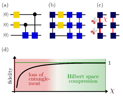
In this work, we use matrix product states to simulate the execution of quantum algorithms on NISQ devices. The idea is illustrated in Fig. 1, showing how the quantum circuit in Fig. 1a is represented by the matrix product states and operators in Fig. 1b. By reducing the bond dimension of the matrix product states, Fig. 1c, we can simulate the generic loss of entanglement and thereby evaluate the fidelity of the quantum algorithms in a noisy quantum circuit. In particular, as illustrated in Fig. 1d, we first reduce the bond dimension, so that unexplored parts of the Hilbert space are removed (green region) without changing the results of our calculations. This reduction of the Hilbert space provides a significant speed-up of our simulations and forms the basis of most calculations based on matrix product states. However, we then further reduce the bond dimension, which not only provides an additional speed-up, but it also removes relevant entangled states (red region), and it thereby mimics the generic loss of entanglement in an actual noisy quantum computer. Using this approach, we evaluate the fidelity of the quantum Fourier transform, Grover’s search algorithm, and the quantum counting algorithm Brassard et al. (1998) with increasing loss of entanglement. The quantum Fourier transform is an important building block for other quantum algorithms such as Shor’s algorithm, while the quantum counting algorithm is a useful application of the more general quantum phase estimation algorithm Kitaev (1995); Nielsen and Chuang (2010). We also investigate the fidelity of the approximate quantum Fourier transform, where small qubit rotations in the exact quantum Fourier transform are omitted Barenco et al. (1996). From a computational point of view, our simulations are efficient, since the quantum algorithms only explore a tiny fraction ($1/10^{4}$) of the Hilbert space, allowing us to work with a low bond dimension, which is then further reduced to describe the generic loss of entanglement. For each algorithm, we map up the entanglement that is generated in the circuit, and we find that all three algorithms can be executed with a high fidelity even at a moderate loss of entanglement.

The paper is organized as follows. In Sec. II, we briefly review the theory of matrix product states and matrix product operators, and we show how they can be used to simulate the execution of quantum algorithms on NISQ computers. In Sec. III, we simulate the execution of the quantum Fourier transform, Grover’s search algorithm, and the quantum counting algorithm on NISQ computers, and we analyze their fidelity as a function of the bond dimension to mimic the loss of entanglement. Finally, in Sec. IV, we provide our conclusions together with an outlook on possible directions for the future. Some technical details are described in two appendixes.

II Tensor-network simulations

Figure 2: Single- and multi-qubit gates. (a) If a single-qubit gate is applied, it is sufficient only to update the tensor for the corresponding qubit. (b) The application of a multi-qubit gate leads to a higher bond dimension, which is then truncated to the largest allowed value. The value of the bond dimension is indicated by the thickness of the connecting lines.

We employ matrix product states to represent the state of a quantum computer as it executes a quantum algorithm Vidal (2004); Schollwoeck (2011). A generic quantum state can be expressed in the computational basis $\{|\bm{\sigma}\rangle=\ket{\sigma_{1},\sigma_{2},...,\sigma_{N}}\}$, where $\sigma_{i}=0,1$ is the value of qubit number $i=1,\ldots,N$. We can then write the state of the quantum computer as

$$\ket{\Psi}=\sum_{\bm{\sigma}}C^{\bm{\sigma}}|\bm{\sigma}\rangle,$$ (1)

where $C^{\bm{\sigma}}$ are the expansion coefficients. Importantly, the expansion coefficients $C^{\bm{\sigma}}$ can be decomposed as a chain of $N$ tensors $A_{i}$, reading

$$C^{\bm{\sigma}}=\sum_{{\bm{\chi}}}[A_{1}]_{\chi_{1}}^{\sigma_{1}}[A_{2}]_{\chi_{1}\chi_{2}}^{\sigma_{2}}...[A_{N}]_{\chi_{N-1}}^{\sigma_{N}},$$ (2)

where the vector $\bm{\chi}=(\chi_{1},\chi_{2},\ldots,\chi_{N-1})$ contains the bond dimensions of each tensor. This representation becomes exact if the bond dimensions $\chi_{i}$ are chosen exponentially large in the system size. In particular, the description of highly-entangled states requires large bond dimensions. For lower bond dimensions, with all bond dimensions bounded from above as $\chi_{j}\leq\chi_{\text{max}}$, highly entangled states are effectively excluded. Thus, in the following, we first reduce the bond dimension so that unexplored parts of the Hilbert space are removed. We then further reduce the bond dimension to mimic the loss of entanglement in an actual noisy quantum computer. All of our calculations are performed with the ITensors package ITe ; Fishman et al. (2022); Niedermeier (2023) and take less than a few hours of computing time on a single-core node. Before proceeding to our simulations, we first briefly discuss the implementation of single- and multi-qubit gates in the framework of matrix product states.

Figure 3: Quantum circuit for the quantum Fourier transform. (a) The quantum Fourier transform, here with $N=4$ qubits, is constructed from Hadamard gates, controlled rotations, and SWAP gates at the end. (b) In the approximate quantum Fourier transform, rotations below a certain angle are omitted so that only nearest-neighbor control is required in this example.

We first consider the application of a (non-entangling) single-qubit gate $M$ to a quantum state $\ket{\Psi}$. Since the gate only acts on a single tensor in the matrix product state, it is sufficient to update this tensor and replace the original tensor $A$ by the updated one $A^{\prime}$ as

$$[A_{i}]_{\chi_{i-1}\chi_{i}}^{\sigma_{i}}\rightarrow\sum_{\sigma_{i}}M^{\sigma_{i}^{\prime}\sigma_{i}}[A_{i}]_{\chi_{i-1}\chi_{i}}^{\sigma_{i}}\equiv[A_{i}^{\prime}]_{\chi_{i-1}\chi_{i}}^{\sigma_{i}^{\prime}}.$$ (3)

Multi-qubit gates are constructed as matrix product operators, which define a parametrization of an operator as

$$O=\sum_{\bm{\sigma},\bm{\sigma^{\prime}}}O^{\bm{\sigma},\bm{\sigma^{\prime}}}\!\ket{\bm{\sigma}}\!\bra{\bm{\sigma^{\prime}}}$$ (4)

in terms of a collection of tensors $W_{i}$, so that

$$O^{\bm{\sigma},\bm{\sigma^{\prime}}}=\sum_{\bm{\chi}}[W_{1}]_{\chi_{1}}^{\sigma_{1},\sigma_{1}^{\prime}}[W_{2}]_{\chi_{1}\chi_{2}}^{\sigma_{2},\sigma_{2}^{\prime}}...[W_{N}]_{\chi_{N-1}}^{\sigma_{N},\sigma_{N}^{\prime}}.$$ (5)

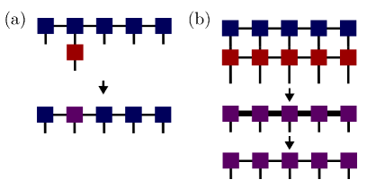
This construction ensures that the structure of the matrix product state is maintained if a matrix product operator is applied. The construction of single- and multi-qubit gates is illustrated in Fig. 2.

In the following, we represent every multi-qubit gate as a matrix product operator, even though gates that act on neighboring qubits could also be represented as rank-$4$ tensors Zhou et al. (2020). However, with this design choice, we can implement multi-qubit controlled gates in a unified manner, which is independent of the separation between the control and the target qubit. When applying a multi-qubit gate, we employ a variational algorithm to find the best approximation of the quantum state for a given maximal bond dimension Schollwoeck (2011); Ayral et al. (2022); Paeckel et al. (2019). The explicit construction of the relevant quantum gates in terms of matrix product operators is described in detail in Appendix A.

Figure 4: Entanglement in the quantum Fourier transform. (a) Quantum circuit for evaluating the fidelity of the quantum Fourier transform. The first gate, $U_{\mathrm{rand}}$, generates a random input state for the quantum Fourier transform (QFT), which is subsequently reversed. The fidelity is given in terms of the overlap between the random input state and the output of the circuit. (b-d) Evolution of the entanglement entropy throughout the circuit with increasing bond dimension, $\chi=25,100,250$.

We can sample from a matrix product state without performing a full contraction to recover the exact state vector Ferris and Vidal (2012); Fishman et al. (2022). Instead, we construct the density matrix $\rho_{i}$ for each qubit, represented by the tensor $A_{i}$, as

$$\left[\rho_{i}\right]^{\sigma_{i},\sigma_{i}^{\prime}}=\sum_{\chi_{i-1},\chi_{i}}[A_{i}]_{\chi_{i-1}\chi_{i}}^{\sigma_{i}}[A_{i}^{\dagger}]_{\chi_{i-1}\chi_{i}}^{\sigma_{i}^{\prime}},$$ (6)

by performing a sweep through the matrix product state representing the final quantum state in the circuit. For each density matrix $\rho_{i}$, we then randomly pick a bit, $r_{i}=0,1$, according to the probabilities defined by the diagonal elements of $\rho_{i}$, corresponding to a single-qubit measurement in the computational basis. Measurement statistics are obtained by repeating this procedure many times and constructing a histogram of the outputs.

Below, we consider the quantum Fourier transform, Grover’s search algorithm, and the quantum counting algorithm. In each case, we briefly review the algorithm before simulating its execution on a NISQ device.

III Quantum Algorithms

III.1 Quantum Fourier transform

The quantum Fourier transform extends the classical discrete Fourier transform to the quantum realm. As its input, it takes a quantum state with $N$ qubits,

$$\ket{\Psi}=\sum_{\bm{\sigma}}C^{\bm{\sigma}}|\bm{\sigma}\rangle=\sum_{l=0}^{2^{N}-1}C_{l}\ket{l},$$ (7)

where we have associated each state in the computational basis with an equivalent decimal number, $\{|\bm{\sigma}\rangle\}=\{\ket{l},|l=0,...,2^{N}-1\}$. The quantum Fourier transform of each basis state is now defined as

$$\mathrm{QFT}\ket{l}=\frac{1}{\sqrt{2^{N}}}\sum_{m=0}^{2^{N}-1}e^{\frac{2\pi i}{2^{N}}lm}\ket{m},$$ (8)

and the transformation of the general state becomes

$$\mathrm{QFT}\ket{\Psi}=\frac{1}{\sqrt{2^{N}}}\sum_{l,m=0}^{2^{N}-1}C_{l}e^{\frac{2\pi i}{2^{N}}lm}\ket{m}.$$ (9)

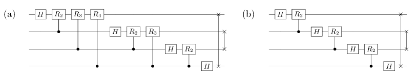
Figure 3a illustrates the circuit representation of the quantum Fourier transform with $N=4$ qubits. The circuit is constructed from controlled rotations of target qubits along the $z$-axis of the Bloch sphere as

$$R_{k}=\begin{bmatrix}1&0\\ 0&e^{\frac{2\pi i}{2^{k}}}\end{bmatrix}$$ (10)

together with SWAP gates at the end that reverse the order of the qubits. For large values of $k$, the rotations are small, and they can, to a good approximation, be neglected Coppersmith (2002); Barenco et al. (1996). That procedure defines the approximate quantum Fourier transform, whose circuit is depicted in Fig. 3b, where controlled rotations with $k>2$ have been omitted. In the following, we first simulate the execution of the quantum Fourier transform on a NISQ device before considering the approximate transformation.

For the classical Fourier transform, one is often interested in a one-to-one mapping between the time domain and the frequency domain, for example, to construct the entire frequency spectrum of an input signal. By contrast, in the context of quantum phase estimation and similar algorithms, the quantum Fourier transform is used to extract a single or a narrow range of frequencies. Approximating a phase with a maximum error of $\epsilon$ requires about $-\lceil\log_{2}(\epsilon)\rceil$ qubits. For instance, a maximum error of $\epsilon=10^{-9}$ requires $30$ qubits, and we will therefore limit our simulation to this number of qubits.

Figure 5: Fidelity of the quantum Fourier transform. (a) The fidelity as a function of the bond dimension for different numbers of qubits. The results are averaged over $10$ random initial states with the standard deviations indicated by error ribbons. (b) The required bond dimension to reach a given fidelity for different numbers of qubits.

It has been observed that the quantum Fourier transform does not rely on a high degree of entanglement Aharonov et al. (2006); Yoran and Short (2007); Woolfe et al. (2014); Chen et al. (2022). The main exception is the use of SWAP gates at the end of the circuit to reorder the qubits. However, if the quantum Fourier transform is performed at the end of an algorithm, one may simply reverse the order in which the qubits are read out by classical means. In the present work, we consider the worst-case scenario, where the input state is random and may have a non-trivial and highly entangled structure. We then define the fidelity as

$$f=|\innerproduct{\Psi_{0}^{\prime}}{\Psi_{0}}|^{2},$$ (11)

where $\ket{\Psi_{0}}$ is the random input state, and

$$\ket{\Psi_{0}^{\prime}}=\mathrm{QFT}^{-1}\mathrm{QFT}\ket{\Psi_{0}}$$ (12)

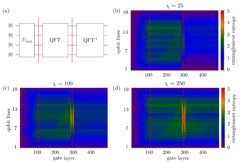
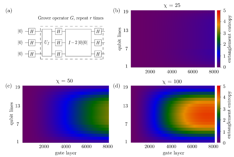
is the state after the quantum Fourier transform has been applied and reversed. In an ideal quantum computer, the fidelity would be one, whereas noise is expected to reduce the fidelity. Figure 4a shows the quantum circuit for obtaining $\ket{\Psi_{0}^{\prime}}$ and finding the fidelity. We initialize the random circuit with $20$ layers of alternating single-qubit gates and CNOT gates Zhou et al. (2020). We keep track of the total number of multi-site gates, such that the generation of the random 20-qubit state in Fig. 4a requires $105$ gate layers. We then average over 10 random states and evaluate the mean and standard deviation of the fidelity.

Before discussing the fidelity, we investigate how the entanglement entropy evolves throughout the quantum circuit. The entanglement entropy is defined as

$$\mathcal{S}_{L}=-\mathrm{Tr}\{\rho_{L}\ln\rho_{L}\},$$ (13)

where $\rho_{L}$ is the reduced density of the first $L$ qubits in the circuit, obtained by tracing out the remaining $N-L$ qubits. The entanglement entropy vanishes for product states, while it has the maximum value of $\mathcal{S}^{\mathrm{max}}_{L}=L\ln{2}$ for highly entangled states of $L\leq N/2$ qubits. For $L>N/2$, the maximum entanglement entropy is $\mathcal{S}^{\mathrm{max}}_{L}=(N-L)\ln{2}$. In Figs. 4b,c,d, we consider a circuit with $N=20$ qubits that we describe using three different bond dimensions. The vertical axis indicates the value of $L$ at which we partition the circuit. We can clearly distinguish three regions, indicated by dashed vertical lines, corresponding to the generation of the random state, the quantum Fourier transform, and its inverse. To begin with, the entanglement grows as an initial state is randomly generated for each panel. The entanglement continues to grow as the quantum Fourier transform is applied, and it reaches its maximum around the SWAP gates. The maximum, however, is only clearly resolved, if the bond dimension is high enough. Only for the highest bond dimension, the entanglement is fully accounted for. Thus, if a quantum Fourier transform is performed on a NISQ device, one can expect a loss of fidelity around the SWAP gates, where the entanglement is concentrated.

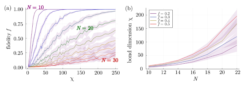
Figure 5 displays the fidelity of the quantum Fourier transform. In Fig. 5a, we show it as a function of the bond dimension for different numbers of qubits. With a small number of qubits, the fidelity quickly approaches one, indicating that it can be carried out on a NISQ device. By contrast, with more qubits, a much higher bond dimension is required, meaning that a low-loss quantum device would be needed. In Fig. 5b, we show the required bond dimension to reach a given fidelity as a function of the qubit number. Importantly, this figure demonstrates that the required bond dimension grows faster than linearly with the number of qubits. Thus, in a quantum computer, it becomes increasingly more demanding to perform a quantum Fourier transform as the circuit size grows.

Figure 6: Controlled rotations. We show the distance between a rotated two-qubit state $\ket{\Psi^{\prime}}=CR_{k}\ket{\Psi}$ and the original state $\ket{\Psi}$ as a function of $k$, which controls the rotation angle. We show the maximum distance for all possible two-qubit states together with the mean and median values, see Appendix B.

Figure 7: Fidelity of the approximate quantum Fourier transform. (a) The fidelity as a function of the bond dimension for $N=20$ qubits and different cut-offs $l$ of the rotations. The results are averaged over 10 random initial states with the standard deviations indicated by error ribbons. (b) The required bond dimension to reach a given fidelity as a function of the cut-off.

To circumvent this issue, we now consider the approximate quantum Fourier transform, where small qubit rotations are neglected. To this end, we first analyze a controlled qubit rotation for different values of $k$. We can write the controlled rotation as

$$CR_{k}=\ket{0}\!\bra{0}\otimes 1+\ket{1}\!\bra{1}\otimes R_{k},$$ (14)

where $R_{k}$ is defined in Eq. (10). A general two-qubit input state can be written as

$$\ket{\Psi}=c_{00}\ket{00}+c_{01}\ket{01}+c_{10}\ket{10}+c_{11}\ket{11},$$ (15)

where the complex coefficients $c_{ij}$ ensure that the state is normalized. To understand the effects of a controlled rotation, we evaluate the distance between the initial state $\ket{\Psi}$ and the rotated state $\ket{\Psi^{\prime}}=CR_{k}\ket{\Psi}$, defined as

$$\delta=1-|\bra{\Psi^{\prime}}\!\Psi\rangle|^{2}.$$ (16)

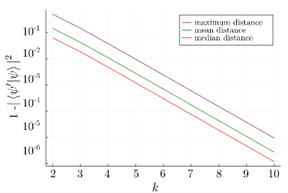
In Fig. 6, we show this distance as a function of the rotation angle, averaged over all possible two-qubit states. The figure shows us that to resolve rotations with $k>4$, one needs a gate fidelity of at least $99\%$. Consequently, with lower gate fidelities, one might as well exclude rotations with $k\geq 5$. Leaving out those gates in a quantum Fourier transform leads to a shallower quantum circuit compared to the full quantum Fourier transform.

In Fig. 7, we show the fidelity of the approximate quantum Fourier transform, which we define as

$$f_{l}=|\innerproduct{\Psi^{\prime}_{0,l}}{\Psi_{0}}|^{2},$$ (17)

where $\ket{\Psi_{0}}$ is the random input state, and

$$\ket{\Psi^{\prime}_{0,l}}=\mathrm{AQFT}_{l}^{-1}\mathrm{QFT}\ket{\Psi_{0}}$$ (18)

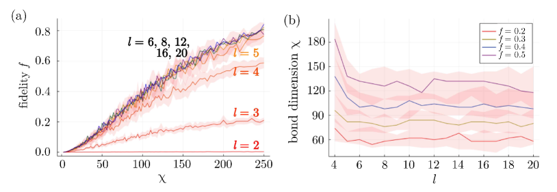
is the state after the quantum Fourier transform and the inverse approximate quantum Fourier transform with $k\leq l$ have been applied. For $l=2$, only controlled nearest-neighbor rotations are included, while $l=N$ corresponds to the exact quantum Fourier transform for a circuit with $N$ qubits. In Fig. 7, we have used $N=20$ qubits, and we see that the fidelity does not approve much as $l$ is increased beyond $l=5$. Thus, in a noisy environment, where entanglement is lost, it makes sense to truncate the rotations and apply the approximate quantum Fourier transform instead of the exact transform.

In Fig. 7b, we show lines of constant fidelity as a function of the cut-off of the rotations. Again, we see that the fidelity of the approximate quantum Fourier transform is roughly constant if the cut-off $l$ is larger than five, noting that the fluctuations are due to different random initial states. In combination, our results demonstrate how the fidelity of the transformation decreases with increasing noise levels. In particular, the entanglement resources required to maintain the fidelity grows super-linearly with the number of qubits. Furthermore, we find that the fidelity of the approximate quantum Fourier transform is similar to the exact transformation if implemented on a noisy quantum computer with loss of entanglement.

Figure 8: Entanglement in Grover’s search algorithm. (a) Quantum circuit for Grover’s algorithm. After the initial state is prepared in an equal superposition, the Grover oracle $U_{f}$ and the Grover diffuser are applied $r$ times to increase the probability of measuring the marked items in the database. We use the optimal number of iterations, which is approximately given by $r\simeq\sqrt{n/m}$ for $m$ marked items in a database with $n$ items. (b,c,d) Evolution of the entanglement entropy throughout the circuit with increasing bond dimension for $m=100$ marked items in a database with $n=2^{20}$ items encoded in $N=20$ qubits.

III.2 Grover’s search algorithm

Grover’s algorithm provides a quadratic speed-up for the task of searching an unsorted database Grover (1996). In the following, we let $n$ denote the number of items in the database and $m$ the number of marked items that we are searching for. A circuit with $N$ qubits can store $n=2^{N}$ items, and the unsorted database is described by the state $\ket{s}=H^{\otimes N}\ket{0}$, which is an equal superposition of all items, and $H$ is the Hadamard gate. We now decompose the state of the database as

$$\ket{s}=\cos(\alpha)\ket{\omega}+\sin(\alpha)\ket{\bar{\omega}},$$ (19)

where we have introduced the angle $\alpha$, so that $\cos(\alpha)=\sqrt{m/n}$ and $\sin(\alpha)=\sqrt{(n-m)/n}$, and $\ket{\omega}$ is an even and normalized superposition of all marked items,

$$\ket{\omega}=\frac{1}{\sqrt{m}}\sum_{i}^{m}\ket{\omega_{i}}.$$ (20)

Similarly, all unmarked items are contained in $\ket{\bar{\omega}}$. To find the marked items, the amplitude of $\ket{\omega}$ must be brought close to one. This amplitude amplification is achieved in two steps Brassard et al. (2000). First, a Grover oracle $U_{f}$ flips the signs of all marked items. Second, a Grover diffuser is applied, which implements a reflection about the equal superposition state as $G_{\mathrm{diff}}=1-2\ket{s}\!\bra{s}=H^{\otimes N}(1-2\ket{0}\!\bra{0})H^{\otimes N}$. The Grover operator $G=G_{\mathrm{diff}}U_{f}$ is now applied to the database $r$ times as depicted in Fig. 8a. This procedure increases the probability of measuring the marked items. The optimal number of Grover iterations depends on the size of the database and the number of marked items and is approximately given by $\sqrt{n/m}$ Grover (1996); Nielsen and Chuang (2010). Thus, the search for a single item requires about $\sqrt{n}$ iterations as compared to a classical algorithm, where $n/2$ iterations are needed on average.

Figure 9: Fidelity of Grover’s algorithm. (a) The fidelity as a function of the bond dimension for different numbers of marked items among a total of $n=2^{20}$ items encoded in $N=20$ qubits. (b) Lines of constant fidelity as functions of the number of marked elements. (c,d) Similar plots as in panels a and b, however, for different numbers of qubits with $m=100$ marked items.

We are now interested in the overlap between the marked items $\ket{\omega_{i}}$ and the state of the circuit after $r$ Grover iterations. Hence, we define the fidelity as

$$f_{r}=\frac{1}{m}\sum_{i}^{m}|\innerproduct{\omega_{i}}{\Psi_{r}}|^{2},$$ (21)

where $\ket{\Psi_{r}}=G^{r}\ket{s}$. If the state $\ket{\Psi_{r}}$ is an even superposition of all marked elements, the fidelity is one. By contrast, it may be reduced below one, if the number of Grover rotations is not optimal, or if the algorithm is executed in a noisy environment with loss of entanglement. In the following, we use the optimal number of iterations, so that the fidelity is close to one for an ideal quantum computer. We then examine how the fidelity is reduced if Grover’s algorithm is executed on a NISQ device.

Before discussing the fidelity, we first consider the entanglement in Grover’s algorithm for different bond dimensions as shown in Figs. 8b,c,d. Figure 8d corresponds to the largest bond dimension, and one clearly sees how the entanglement in the circuit builds up as the number of Grover iterations approaches the optimal value. Thus, right before the state of the system is read out, the entanglement reaches its maximum, which is given by the entanglement in the superposition of all marked items. In the other panels, the bond dimension is lower, and the entanglement is partially lost. As such, we expect a significant reduction of the corresponding fidelity.

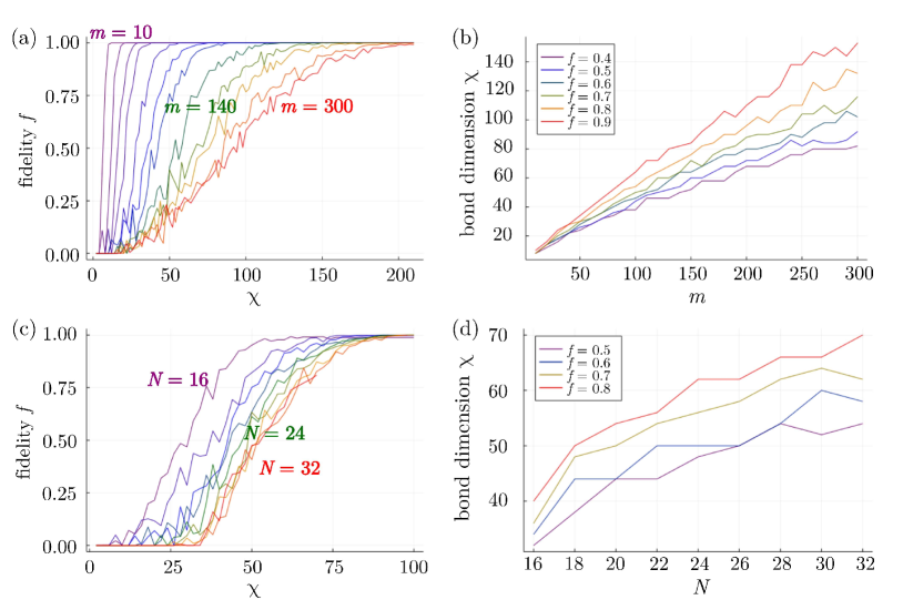
Figure 9 shows the fidelity of Grover’s algorithm in a noisy environment. In Fig. 9a, we show the fidelity as a function of the bond dimension for different numbers of marked items, which are drawn randomly at the beginning of each simulation Figgatt et al. (2017); Mermin (2007). For different numbers of marked items, we average the results over $10$ random draws. The fluctuations in the results stem from two effects. First, since the marked items are generally different, the Grover operator will also be constructed in different ways. Therefore, it will be affected slightly differently by the truncation procedure to reduce the bond dimension. Second, the optimal number of rotations $r_{\text{opt}}$ is only defined up to an integer, and the final state in Grover’s algorithm may not have complete overlap with the marked items in the state $\ket{\omega}$.

Figure 10: Entanglement in the quantum counting algorithm. (a) Quantum circuit for the quantum counting algorithm, which is equivalent to a quantum phase estimation applied to the Grover operator. The initial state is rotated into an equal superposition of all items in the database, which is the sum of two eigenstates of the Grover operator. (b,c,d) Entanglement entropy in the circuit for different bond dimensions with $N=20$ qubits and $m=30$ marked items of a total of $n=2^{10}=1024$ items.

With a low number of marked items, the fidelity abruptly approaches one beyond a certain threshold, which can even be remarkably low. By contrast, for larger numbers of marked items, the fidelity increases more slowly with the bond dimension. Figure 9b illustrates how the required bond dimension to achieve a certain fidelity grows approximately linearly with the number of marked items. This behavior can be contrasted with that of the quantum Fourier transform, where a super-linear growth of the bond dimension with increasing system size is observed. Figures 9c,d show the dependence of the fidelity on the bond dimension for different numbers of qubits and a fixed number of marked items. Also, in this case, we observe that Grover’s algorithm can be executed with high fidelity for low bond dimensions. We note that the required bond dimension to achieve a given fidelity depends roughly linearly on the number of qubits, indicating that Grover’s algorithm is more resilient to noise as compared to the quantum Fourier transform, where the dependence is stronger. Furthermore, increasing the size of the search space (even considerably) requires only a very modest increase in the bond dimension in order to achieve the same fidelity, as shown explicitly in Fig. 9d. Upon increasing the dimension of the search space from $2^{16}\simeq 6\times 10^{4}$ to $2^{32}\simeq 4\times 10^{9}$, an increase of only $20$-$30$ in the bond dimension is required to maintain a high fidelity. Altogether, this indicates that Grover’s algorithm is considerably more resilient to an increase in the total search space size than to an increase in the number of elements that one seeks to identify. In both cases, however, results with high fidelity have been obtained for comparatively low bond dimensions. The quantum advantage in Grover’s algorithm is therefore rather rooted in the efficient use of quantum superpositions than in exploiting entanglement resources. Regarding the computational costs of our simulations, it is worth mentioning that a bond dimension of $\chi=100$ implies that only a tiny part of the Hilbert space is explored by the quantum algorithm, and, in the case of 32 qubits, this fraction can be estimated to be

$$\text{fraction of Hilbert space}=\frac{2\times 32\times\chi^{2}}{2^{32}}\simeq 10^{-4}.$$ (22)

In our simulation, the bond dimension is further reduced below $\chi=100$ to simulate the generic loss of entanglement in a quantum computer.

To summarize, Grover’s algorithm can be executed with high fidelity using a rather low bond dimension, in particular for a small number of marked items. As the number of marked items and the size of the database grow, the required bond dimension to achieve a given fidelity only increases linearly. For this reason, Grover’s algorithm appears to be less sensitive to the loss of entanglement as compared to the quantum Fourier transform.

III.3 Quantum counting algorithm

Figure 11: Output of the quantum counting algorithm. (a,b,c) For illustration, we consider a database with 30 out of 128 items marked. In the Fourier register, 4 out of 5 qubits are measured, so that the phases can be determined with up to 4 binary digits corresponding to a precision of $1/2^{4}\simeq 0.06$. The correct phases are marked in red. The panels correspond to different bond dimensions.

Figure 12: Accuracy of the quantum counting algorithm. (a,b) The number of marked items as determined by the quantum counting algorithm compared to the actual number as a function of the bond dimension. The lines correspond to different numbers of qubits in the quantum Fourier transform, while the Grover operator in each case is applied to 10 qubits. We consider $m=20$ and $m=40$ marked items in the two panels. (c,d) In these panels, we use the approximate quantum Fourier transform instead of the exact one, and we show results for different values of the truncation number $l$.

The problem of determining the number of marked items in a database, given a Grover operator, is solved by the quantum counting algorithm. It may also be applied to more general problems that can be recast as search problems Brassard et al. (1998); Nielsen and Chuang (2010). The quantum counting algorithm is an application of the quantum phase estimation algorithm, which can determine the eigenvalues of a unitary operator given the corresponding eigenstates. In the following, the operator whose eigenvalues we seek is the Grover operator. In the subspace spanned by $\ket{\omega}$ and $\ket{\bar{\omega}}$, the Grover operator can be represented by the matrix

$$G=\begin{bmatrix}\cos(2\alpha)&-\sin(2\alpha)\\ \sin(2\alpha)&\cos(2\alpha)\end{bmatrix}$$ (23)

with eigenvalues $\lambda_{\pm}=e^{\pm 2\alpha i}$ and corresponding eigenvectors $\ket{\pm}=(\pm\ket{\omega}+i\ket{\bar{\omega}})/\sqrt{2}$. The state of the database can be expressed as a superposition of these eigenstates,

$$\ket{s}=(e^{-i\alpha}\ket{+}-e^{i\alpha}\ket{-})/\sqrt{2},$$ (24)

which is the starting point for the quantum phase estimation algorithm to find the two eigenvalues. Once we have determined the phases of the eigenvalues, $\pm 2\alpha$, we obtain the number of marked items as Brassard et al. (1998); Nielsen and Chuang (2010)

$$m=n\sin^{2}(\alpha),$$ (25)

and the optimal number of iterations follows as

$$r_{\text{opt}}=\Bigg{\lceil}\frac{\pi}{4}\sqrt{\frac{n}{m}}\Bigg{\rceil}.$$ (26)

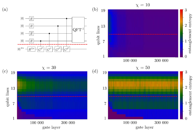
Figure 10a shows the circuit for the quantum counting algorithm. The quantum phase estimation is implemented as described in Ref. Nielsen and Chuang (2010). The dashed red line separates an upper register, where the phases of the eigenvalues get encoded, and a lower one, where the Grover operator is applied. The phases are read out after the inverse quantum Fourier transform by measuring the first $N_{\mathrm{read}}$ qubits of the top register, which yields the phases with up to $N_{\mathrm{read}}$ binary digits. The output state has to be measured several times to construct a histogram of the outcomes, which will be peaked around the two phases. If the phases should be found with a probability of at least $1-\epsilon$, one has to construct the top register with

$$N_{\mathrm{aux}}=\lceil\log_{2}(2+1/2\epsilon)\rceil$$ (27)

auxiliary qubits, which are not measured at the end of the quantum phase estimation routine. The uncertainty in the number of marked items can be estimated as

$$\Delta m=\left(\sqrt{2mn}+n/2^{N_{\mathrm{read}}+1}\right)/2^{N_{\mathrm{read}}},$$ (28)

which decreases with the number of qubits measured in the top register. By contrast, the success probability increases with the number of auxiliary qubits, which are not measured, according to Eq. (27). For the following, we take $N_{\mathrm{aux}}=2$ corresponding to $\epsilon\simeq 0.09$.

In Figs. 10b,c,d, we show how the entanglement evolves throughout the circuit for different bond dimensions. Starting with the highest bond dimension in Fig. 10d, we see that the entanglement is concentrated in the upper register, which is conditioned on applications of the Grover operator in the lower register. In practice, this observation implies that the qubits with the highest fidelity should be used for the upper register since less entanglement is needed in the lower one. In Fig. 10b,c, the bond dimension is further reduced, leading to a loss of entanglement in the circuit as we see.

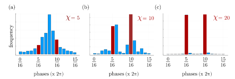
In the quantum counting algorithm, the state of the upper register is measured and converted into an approximation of the two phases, $\pm 2\alpha$. The algorithm is executed several times, and a histogram as shown in Fig. 11 is generated. To determine the phases, we use a randomized method instead of simply selecting the two most probable values in the histogram. Instead, we randomly pick a value in the histogram based on its probability, and we then average over a large number of independent draws from the distribution. This method has the advantage of better dealing with statistical fluctuations for low bond dimensions, where the histogram might not be clearly peaked around the correct phases. With a high enough bond dimension, the method is effectively equivalent to simply selecting the two most probable phases.

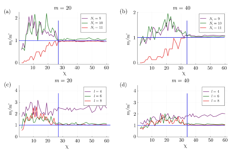
The main outcome of the quantum counting algorithm is the number of marked items, and we now investigate how it depends on the bond dimension. To this end, we consider a $10$-qubit Grover register, corresponding to a database with $n=2^{10}=1024$ items, together with $m=20$ or $40$ marked items. Between $6$ and $11$ qubits are used for the quantum Fourier transform with the last two of them not being measured as it increases the overall success probability. In Fig. 12, we show the number of marked items determined by the quantum counting algorithm over the actual number of marked items as a function of the bond dimension. In Figs. 12a,b, we consider $m=20$ and $m=40$ marked items in the database, respectively. The different lines correspond to varying numbers of qubits in the top register, which are used for the inverse quantum Fourier transform at the end of the algorithm. For large bond dimensions, the algorithm predicts the correct number of marked items, and the lines converge to one. This behavior depends only weakly on the number of qubits $N_{t}$ in the quantum Fourier register. We note that the small fluctuations are due to the inherent quantum fluctuations and the probabilistic nature of the algorithm Brassard et al. (1998); Nielsen and Chuang (2010). While our simulations in principle are deterministic, there are fluctuations because of simulated measurements at the end of the circuit.

In Figs. 12c,d, we show similar results, but this time using the approximate quantum Fourier transform instead of the full quantum Fourier transform. We use a quantum Fourier register with $N_{t}=10$ qubits and vary the truncation number of the approximate quantum Fourier transform between. With a truncation number of $l=6,8$, the results are similar to those obtained with the exact quantum Fourier transform. By contrast, for $l=4$, the algorithm does not identify the correct number of marked items because of the limited fidelity of the approximate quantum Fourier transform. Thus, we find that the quantum Fourier transform may be truncated to a gate fidelity of $99\%$ ($l=6$) and still yield the correct eigenvalues.

IV Conclusions

We have simulated the execution of three quantum algorithms on NISQ devices using matrix product states with a finite bond dimension to mimic the loss of entanglement in an actual quantum computer. Specifically, we have considered the quantum Fourier transform, Grover’s search algorithm, and the quantum counting algorithm. In all three cases, we have found that the algorithms can be executed with high fidelity even at a moderate loss of entanglement. Our simulations also make it possible to map out the entanglement that is generated throughout the execution of an algorithm, allowing us to identify the regions of a circuit with the largest entanglement. For the quantum Fourier transform and Grover’s algorithm, we have found that the fidelities decrease with the loss of entanglement. However, for the quantum Fourier transform, the relationship is not linear in the system size. Larger systems require more entanglement to reach the same fidelity. For the quantum counting algorithm, we have investigated how the prediction of the number of marked items depends on the loss of entanglement. Here we have found that the exact number can be predicted even with rather low bond dimensions. This observation suggests that algorithms that are based on the quantum phase estimation can be executed even with a moderate loss of entanglement. We have also found that one may replace the quantum Fourier transform with its approximate version and still reliably determine the phases in the quantum counting algorithm. In addition to mimicking the loss of entanglement in a NISQ device, the reduced bond dimension also made our simulations numerically feasible, and most of them were performed on a single-core node in a few hours of computing time.

Our work shows how the execution of quantum algorithms on NISQ devices can be emulated using matrix product states. In the future, it can be extended in several directions. While a reduced bond dimension may describe the generic loss of entanglement in a noisy quantum computer, more refined descriptions could be developed where the loss of entanglement is attributed to specific microscopic processes in a particular type of quantum computer. Also, while the reduced bond dimension only describes the loss of entanglement, it may be interesting to include the decoherence of superposition states that are not entangled such as the initial state of Grover’s algorithm. Having implemented two of the most basic quantum subroutines, namely the quantum Fourier transform and the quantum phase estimation, an obvious next step would be to investigate the performance of more complex algorithms that are built on these subroutines, for example, Shor’s algorithm or the HHL algorithm to solve systems of linear equations Harrow et al. (2009). Moreover, it would be important to analyze hybrid quantum-classical algorithms such as the variational quantum eigensolver Peruzzo et al. (2014); Endo et al. (2021); Xu et al. (2022), as this would provide a crucial stepping stone for assessing the feasibility of quantum many-body calculations on NISQ hardware.

V Acknowledgments

We acknowledge the computational resources provided by the Aalto Science-IT project as well as the financial support from InstituteQ, the Jane and Aatos Erkko Foundation, and the Academy of Finland through the Finnish Centre of Excellence in Quantum Technology (project numbers 352925 and 336810) and grant numbers 331342, 336243, and 308515.

Appendix A Controlled quantum gates

Here we provide a construction of single-qubit gates that are controlled by a number of other qubits. In particular, we show that they can be represented by a matrix product operator with a bond dimension of three. We note that bond dimensions of two have been achieved for similar matrix product operators, but we will not pursue this approach here Gelß et al. (2022).

To construct the matrix product operator, we consider a gate $U_{j}$ that acts on qubit $j$ and is controlled by $L$ other qubits that we label as $i_{1},i_{2},...,i_{L}$. The gate is applied if all of the control qubits are in the state $\ket{1}$. The controlled operator can be written as

$$\begin{split}C_{i_{1},i_{2},...,i_{L}}U_{j}&=I_{1}\otimes\cdots I_{i_{1}}\cdots I_{j}\cdots I_{i_{L}}\cdots\otimes I_{N}\\ -&I_{1}\otimes\cdots\ket{1}\!\bra{1}_{i_{1}}\cdots I_{j}\cdots\ket{1}\bra{1}_{i_{L}}\cdots\otimes I_{N}\\ +&I_{1}\otimes\cdots\ket{1}\!\bra{1}_{i_{1}}\cdots U_{j}\cdots\ket{1}\!\bra{1}_{i_{L}}\cdots\otimes I_{N},\\ \end{split}$$ (29)

where the first line expresses that the operator generally acts trivially on the qubits. Only if all control qubits are in the state $\ket{1}$, the gate $U_{j}$ is applied to the target qubit instead of $I_{j}$ as expressed by the two other lines.

Similar to the conversion of a locally interacting Hamiltonian into the form of a matrix product operator Hubig et al. (2017), we can now find the abstract tensors in matrix form, which can be multiplied to obtain the three terms in the expression above. For the sake of concreteness, we show the construction for the five-qubit operator $C_{1,4,5}\,X_{3}$,

$$\underset{\text{control}}{\begin{bmatrix}I_{1}\\ -P_{1}\\ P_{1}\\ \end{bmatrix}^{T}}\underset{\text{spectator}}{\begin{bmatrix}I_{2}&&\\ &I_{2}&\\ &&I_{2}\\ \end{bmatrix}}\underset{\text{target}}{\begin{bmatrix}I_{3}&&\\ &I_{3}&\\ &&X_{3}\\ \end{bmatrix}}\underset{\text{control}}{\begin{bmatrix}I_{4}&&\\ &P_{1}&\\ &&P_{1}\\ \end{bmatrix}}\underset{\text{control}}{\begin{bmatrix}I_{5}\\ P_{1}\\ P_{1}\\ \end{bmatrix}},$$ (30)

where $P_{1}=\ket{1}\!\bra{1}$ is a projector, the second qubit is just a spectator qubit, and the multiplication of individual entries should be understood as tensor products.

Evaluating these matrix products indeed yields the correct form of the operator. A generalization to more control qubits as well as qubit registers of different sizes is straightforward by inserting the corresponding matrices for the control and the spectator qubits. Furthermore, this construction can be extended to several controlled single-qubit operators by replacing a spectator tensor with an additional target tensor as

$$\underset{\text{spectator}}{\begin{bmatrix}I_{i}&&\\ &I_{i}&\\ &&I_{i}\\ \end{bmatrix}}\rightarrow\underset{\text{target}}{\begin{bmatrix}I_{i}&&\\ &I_{i}&\\ &&U_{i}\\ \end{bmatrix}}.$$ (31)

With this approach, one can construct any controlled gate as a matrix product operator of bond dimension three (since the matrices above are of rank three). Hence, we can implement all the operators that we need for quantum computations, namely single-qubit gates and controlled gates, with relatively low computational costs.

Appendix B General two-qubit state

Here we provide additional details of our calculations in Fig. 6. By imposing that the two-qubit state in Eq. (15) is normalized and invariant under global phase shifts, we may write the expansion coefficients as

$$\begin{split}c_{00}&=\cos{\phi_{1}},\\ c_{01}&=\sin{\phi_{1}}\cos{\phi_{2}}e^{i\Phi_{1}},\\ c_{10}&=\sin{\phi_{1}}\sin{\phi_{2}}\cos{\phi_{3}}e^{i\Phi_{2}},\\ c_{11}&=\sin{\phi_{1}}\sin{\phi_{2}}\sin{\phi_{3}}e^{i\Phi_{3}}\end{split}$$ (32)

where the parameters $\phi_{1},\phi_{2}$ run in the interval $[0,\pi]$, and $\phi_{3},\Phi_{1},\Phi_{2},\Phi_{3}$ in the interval $[0,2\pi)$. This parametrization can be obtained by representing each coefficient $c_{ij}$ in polar form as $r_{ij}\exp(i\phi_{ij})$, with both $r_{ij}$ and $\phi_{ij}$ being real numbers. Since $\sum_{ij}|r_{ij}|^{2}=1$, we may represent the $r$-coordinates as spherical coordinates on a $4$-sphere, which yields the explicit dependence on the sine- and cosine functions. Factoring out a global phase factor, e.g. $\exp(i\phi_{00})$, and redefining the other phase angles accordingly, we arrive at the parametrization above.

We may then calculate the overlap between any initial state $\ket{\Psi}$ and the rotated state $\ket{\Psi^{\prime}}=CR_{k}\ket{\Psi}$, and we find

$$\begin{split}|\bra{\Psi^{\prime}}\!\Psi\rangle|^{2}=\Bigg{[}\cos^{2}(\phi_{1})+\sin^{2}(\phi_{1})\cos^{2}(\phi_{2})&+\sin^{2}(\phi_{1})\sin^{2}(\phi_{2})\cos^{2}(\phi_{3})+\sin^{2}(\phi_{1})\sin^{2}(\phi_{2})\sin^{2}(\phi_{3})\cos(\frac{2\pi}{2^{k}})\Bigg{]}^{2}\\ &+\Bigg{[}\sin^{2}(\phi_{1})\sin^{2}(\phi_{2})\sin^{2}(\phi_{3})\sin(\frac{2\pi}{2^{k}})\Bigg{]}^{2},\end{split}$$ (33)

which turns out to be independent of the phases $\Phi_{1},\Phi_{2}$ and $\Phi_{3}$. Using this expression, we can calculate the maximum distance and the mean and median values shown in Fig. 6.

References

- Preskill (2018) J. Preskill, Quantum computing in the NISQ era and beyond, Quantum 2, 79 (2018).
- Cheng et al. (2023) B. Cheng, X.-H. Deng, X. Gu, Y. He, G. Hu, P. Huang, J. Li, B.-C. Lin, D. Lu, Y. Lu, C. Qiu, H. Wang, T. Xin, S. Yu, M.-H. Yung, J. Zeng, S. Zhang, Y. Zhong, X. Peng, F. Nori, and D. Yu, Noisy intermediate-scale quantum computers, Front. Phys. 18, 21308 (2023).
- IBM (2022a) IBM unveils 400 qubit-plus quantum processor and next-generation IBM Quantum System two (2022a), accessed: 2022-11-23.
- IBM (2022b) IBM Quantum Computing: Roadmap (2022b), accessed: 2022-11-23.
- Goo (2023) Unveiling our new quantum ai campus (2023), accessed: 2023-1-4.
- (6) P. Shor, Algorithms for quantum computation: discrete logarithms and factoring, in Proceedings 35th Annual Symposium on Foundations of Computer Science (IEEE Comput. Soc. Press).
- Grover (1996) L. K. Grover, A fast quantum mechanical algorithm for database search, in Proceedings of the twenty-eighth annual ACM symposium on Theory of computing - STOC '96 (ACM Press, 1996).
- Coppersmith (2002) D. Coppersmith, An approximate Fourier transform useful in quantum factoring (2002), arXiv:quant-ph/0201067 [quant-ph] .
- Harrow et al. (2009) A. W. Harrow, A. Hassidim, and S. Lloyd, Quantum Algorithm for Linear Systems of Equations, Phys. Rev. Lett. 103, 150502 (2009).
- Francis et al. (2021) A. Francis, D. Zhu, C. H. Alderete, S. Johri, X. Xiao, J. K. Freericks, C. Monroe, N. M. Linke, and A. F. Kemper, Many-body thermodynamics on quantum computers via partition function zeros, Sci. Adv. 7, 10.1126/sciadv.abf2447 (2021).
- Krishnan et al. (2019) A. Krishnan, M. Schmitt, R. Moessner, and M. Heyl, Measuring complex-partition-function zeros of Ising models in quantum simulators, Phys. Rev. A 100, 022125 (2019).
- Murta et al. (2020) B. Murta, G. Catarina, and J. Fernández-Rossier, Berry phase estimation in gate-based adiabatic quantum simulation, Phys. Rev. A 101, 020302 (2020).
- Koh et al. (2022) J. M. Koh, T. Tai, and C. H. Lee, Simulation of Interaction-Induced Chiral Topological Dynamics on a Digital Quantum Computer, Phys. Rev. Lett. 129, 140502 (2022).
- Bharti et al. (2022) K. Bharti, A. Cervera-Lierta, T. H. Kyaw, T. Haug, S. Alperin-Lea, A. Anand, M. Degroote, H. Heimonen, J. S. Kottmann, T. Menke, W.-K. Mok, S. Sim, L.-C. Kwek, and A. Aspuru-Guzik, Noisy intermediate-scale quantum algorithms, Rev. Mod. Phys. 94, 015004 (2022).
- Huang et al. (2022) H.-L. Huang, X.-Y. Xu, C. Guo, G. Tian, S.-J. Wei, X. Sun, W.-S. Bao, and G.-L. Long, Near-Term Quantum Computing Techniques: Variational Quantum Algorithms, Error Mitigation, Circuit Compilation, Benchmarking and Classical Simulation (2022), arXiv:2211.08737 [quant-ph] .
- Bouland et al. (2022) A. Bouland, B. Fefferman, Z. Landau, and Y. Liu, Noise and the frontier of quantum supremacy, in 2021 IEEE 62nd Annual Symposium on Foundations of Computer Science (FOCS) (2022) pp. 1308–1317.
- Lee et al. (2022) S. Lee, J. Lee, H. Zhai, Y. Tong, A. M. Dalzell, A. Kumar, P. Helms, J. Gray, Z.-H. Cui, W. Liu, M. Kastoryano, R. Babbush, J. Preskill, D. R. Reichman, E. T. Campbell, E. F. Valeev, L. Lin, and G. Kin-Lic Chan, Is there evidence for exponential quantum advantage in quantum chemistry? (2022), arXiv:2208.02199 [physics.chem-ph] .
- Baxter (1968) R. J. Baxter, Dimers on a Rectangular Lattice, J. Math. Phys. 9, 650 (1968).
- Fannes et al. (1992) M. Fannes, B. Nachtergaele, and R. F. Werner, Finitely correlated states on quantum spin chains, Commun. Math. Phys. 144, 443 (1992).
- Vidal (2004) G. Vidal, Efficient Simulation of One-Dimensional Quantum Many-Body Systems, Phys. Rev. Lett. 93, 040502 (2004).
- Schollwoeck (2011) U. Schollwoeck, The density-matrix renormalization group in the age of matrix product states, Ann. Phys. 326, 96 (2011).
- Biamonte and Bergholm (2017) J. Biamonte and V. Bergholm, Tensor Networks in a Nutshell (2017), arXiv:1708.00006 [quant-ph] .
- Okunishi et al. (2022) K. Okunishi, T. Nishino, and H. Ueda, Developments in the Tensor Network — from Statistical Mechanics to Quantum Entanglement, J. Phys. Soc. Jpn. 91, 062001 (2022).
- Zhou et al. (2020) Y. Zhou, E. M. Stoudenmire, and X. Waintal, What Limits the Simulation of Quantum Computers?, Phys. Rev. X 10, 041038 (2020).
- Ayral et al. (2022) T. Ayral, T. Louvet, Y. Zhou, C. Lambert, E. Miles Stoudenmire, and X. Waintal, A density-matrix renormalization group algorithm for simulating quantum circuits with a finite fidelity (2022), arXiv:2207.05612 [quant-ph] .
- Cheng et al. (2021) S. Cheng, C. Cao, C. Zhang, Y. Liu, S.-Y. Hou, P. Xu, and B. Zeng, Simulating noisy quantum circuits with matrix product density operators, Phys. Rev. Res. 3, 023005 (2021).
- Noh et al. (2020) K. Noh, L. Jiang, and B. Fefferman, Efficient classical simulation of noisy random quantum circuits in one dimension, Quantum 4, 318 (2020).
- Brennan et al. (2021) J. Brennan, M. Allalen, D. Brayford, K. Hanley, L. Iapichino, L. J. O'Riordan, M. Doyle, and N. Moran, Tensor network circuit simulation at exascale, in 2021 IEEE/ACM Second International Workshop on Quantum Computing Software (QCS) (IEEE, 2021).
- McCaskey et al. (2018) A. McCaskey, E. Dumitrescu, M. Chen, D. Lyakh, and T. Humble, Validating quantum-classical programming models with tensor network simulations, PLOS ONE 13, e0206704 (2018).
- Zhao et al. (2021) Y.-Q. Zhao, R.-G. Li, J.-Z. Jiang, C. Li, H.-Z. Li, E.-D. Wang, W.-F. Gong, X. Zhang, and Z.-Q. Wei, Simulation of quantum computing on classical supercomputers with tensor-network edge cutting, Phys. Rev. A 104, 032603 (2021).
- Zhang et al. (2022) S.-X. Zhang, J. Allcock, Z.-Q. Wan, S. Liu, J. Sun, H. Yu, X.-H. Yang, J. Qiu, Z. Ye, Y.-Q. Chen, C.-K. Lee, Y.-C. Zheng, S.-K. Jian, H. Yao, C.-Y. Hsieh, and S. Zhang, TensorCircuit: a Quantum Software Framework for the NISQ Era (2022), arXiv:2205.10091 [quant-ph] .
- Seitz et al. (2022) P. Seitz, I. Medina, E. Cruz, Q. Huang, and C. B. Mendl, Simulating quantum circuits using tree tensor networks (2022), arXiv:2206.01000 [quant-ph] .
- Pan and Zhang (2022) F. Pan and P. Zhang, Simulation of Quantum Circuits Using the Big-Batch Tensor Network Method, Phys. Rev. Lett. 128, 030501 (2022).
- Pan et al. (2022) F. Pan, K. Chen, and P. Zhang, Solving the Sampling Problem of the Sycamore Quantum Circuits, Phys. Rev. Lett. 129, 090502 (2022).
- Huang et al. (2020) C. Huang, F. Zhang, M. Newman, J. Cai, X. Gao, Z. Tian, J. Wu, H. Xu, H. Yu, B. Yuan, M. Szegedy, Y. Shi, and J. Chen, Classical Simulation of Quantum Supremacy Circuits (2020), arXiv:2005.06787 [quant-ph] .
- Oh et al. (2021) C. Oh, K. Noh, B. Fefferman, and L. Jiang, Classical simulation of lossy boson sampling using matrix product operators, Phys. Rev. A 104, 022407 (2021).
- Pang et al. (2020) Y. Pang, T. Hao, A. Dugad, Y. Zhou, and E. Solomonik, Efficient 2d tensor network simulation of quantum systems, in SC20: International Conference for High Performance Computing, Networking, Storage and Analysis (2020) pp. 1–14.
- Luchnikov et al. (2021) I. A. Luchnikov, A. V. Berezutskii, and A. K. Fedorov, Simulating quantum circuits using the multi-scale entanglement renormalization ansatz (2021), arXiv:2112.14046 [quant-ph] .
- Schutski et al. (2020) R. Schutski, T. Khakhulin, I. Oseledets, and D. Kolmakov, Simple heuristics for efficient parallel tensor contraction and quantum circuit simulation, Phys. Rev. A 102, 062614 (2020).
- Wang et al. (2017) D. S. Wang, C. D. Hill, and L. C. L. Hollenberg, Simulations of Shor’s algorithm using matrix product states, Quantum Inf. Process. 16, 10.1007/s11128-017-1587-x (2017).
- Woolfe et al. (2014) K. J. Woolfe, C. D. Hill, and L. C. L. Hollenberg, Scale invariance and efficient classical simulation of the quantum Fourier transform (2014), arXiv:1406.0931 [quant-ph] .
- Stoudenmire and Waintal (2023) E. M. Stoudenmire and X. Waintal, Grover’s Algorithm Offers No Quantum Advantage (2023), arXiv:2303.11317 [quant-ph] .
- Terhal and DiVincenzo (2002) B. M. Terhal and D. P. DiVincenzo, Adaptive Quantum Computation, Constant Depth Quantum Circuits and Arthur-Merlin Games (2002), arXiv:quant-ph/0205133 [quant-ph] .
- Yoran (2008) N. Yoran, Efficiently contractable quantum circuits cannot produce much entanglement (2008), arXiv:0802.1156 [quant-ph] .
- Jozsa (2006) R. Jozsa, On the simulation of quantum circuits (2006), arXiv:quant-ph/0603163 [quant-ph] .
- Markov and Shi (2008) I. L. Markov and Y. Shi, Simulating quantum computation by contracting tensor networks, SIAM Journal on Computing 38, 963 (2008).
- Gelß et al. (2022) P. Gelß, S. Klus, Z. Shakibaei, and S. Pokutta, Low-rank tensor decompositions of quantum circuits (2022), arXiv:2205.09882 [quant-ph] .
- Wahl and Strelchuk (2022) T. B. Wahl and S. Strelchuk, Simulating quantum circuits using efficient tensor network contraction algorithms with subexponential upper bound (2022), arXiv:2208.01498 [quant-ph] .
- Chen et al. (2022) J. Chen, E. M. Stoudenmire, and S. R. White, The Quantum Fourier Transform Has Small Entanglement (2022), arXiv:2210.08468 [quant-ph] .
- Ma and Yang (2022) L. Ma and C. Yang, Low rank approximation in simulations of quantum algorithms, J. Comp. Sci 59, 101561 (2022).
- Brassard et al. (1998) G. Brassard, P. Høyer, and A. Tapp, Quantum counting, in Automata, Languages and Programming (Springer Berlin Heidelberg, 1998) pp. 820–831.
- Kitaev (1995) A. Y. Kitaev, Quantum measurements and the Abelian Stabilizer Problem (1995), arXiv:quant-ph/9511026 [quant-ph] .
- Nielsen and Chuang (2010) M. A. Nielsen and I. L. Chuang, Quantum Computation and Quantum Information: 10th Anniversary Edition (Cambridge University Press, 2010).
- Barenco et al. (1996) A. Barenco, A. Ekert, K.-A. Suominen, and P. Törmä, Approximate quantum Fourier transform and decoherence, Phys. Rev. A 54, 139 (1996).
- (55) ITensor Library .
- Fishman et al. (2022) M. Fishman, S. R. White, and E. M. Stoudenmire, The ITensor Software Library for Tensor Network Calculations, SciPost Phys. Codebases , 4 (2022).
- Niedermeier (2023) M. Niedermeier, Mps quantum simulation package (2023), accessed: 2023-03-06.
- Paeckel et al. (2019) S. Paeckel, T. Köhler, A. Swoboda, S. R. Manmana, U. Schollwöck, and C. Hubig, Time-evolution methods for matrix-product states, Ann. Phys. 411, 167998 (2019).
- Ferris and Vidal (2012) A. J. Ferris and G. Vidal, Perfect sampling with unitary tensor networks, Phys. Rev. B 85, 165146 (2012).
- Aharonov et al. (2006) D. Aharonov, Z. Landau, and J. Makowsky, The quantum FFT can be classically simulated (2006), arXiv:quant-ph/0611156 [quant-ph] .
- Yoran and Short (2007) N. Yoran and A. J. Short, Efficient classical simulation of the approximate quantum Fourier transform, Phys. Rev. A 76, 042321 (2007).
- Brassard et al. (2000) G. Brassard, P. Hoyer, M. Mosca, and A. Tapp, Quantum Amplitude Amplification and Estimation (2000), arXiv:quant-ph/0005055 [quant-ph] .
- Figgatt et al. (2017) C. Figgatt, D. Maslov, K. A. Landsman, N. M. Linke, S. Debnath, and C. Monroe, Complete 3-qubit grover search on a programmable quantum computer, Nature Commun. 8, 10.1038/s41467-017-01904-7 (2017).
- Mermin (2007) N. D. Mermin, Quantum Computer Science (Cambridge University Press, 2007).
- Peruzzo et al. (2014) A. Peruzzo, J. McClean, P. Shadbolt, M.-H. Yung, X.-Q. Zhou, P. J. Love, A. Aspuru-Guzik, and J. L. O’Brien, A variational eigenvalue solver on a photonic quantum processor, Nature Commun. 5, 10.1038/ncomms5213 (2014).
- Endo et al. (2021) S. Endo, Z. Cai, S. C. Benjamin, and X. Yuan, Hybrid Quantum-Classical Algorithms and Quantum Error Mitigation, J. Phys. Soc. Jpn. 90, 032001 (2021).
- Xu et al. (2022) Z. Xu, Y. Fan, H. Shang, and C. Guo, Differentiable matrix product states for simulating variational quantum computational chemistry (2022), arXiv:2211.07983 [quant-ph] .
- Hubig et al. (2017) C. Hubig, I. P. McCulloch, and U. Schollwöck, Generic construction of efficient matrix product operators, Phys. Rev. B 95, 035129 (2017).