On Mitigating the Utility-Loss in Differentially Private Learning: A New Perspective by a Geometrically Inspired Kernel Approach

Abstract

Privacy-utility tradeoff remains as one of the fundamental issues of differentially private machine learning. This paper introduces a geometrically inspired kernel-based approach to mitigate the accuracy-loss issue in classification. In this approach, a representation of the affine hull of given data points is learned in Reproducing Kernel Hilbert Spaces (RKHS). This leads to a novel distance measure that hides privacy-sensitive information about individual data points and improves the privacy-utility tradeoff via significantly reducing the risk of membership inference attacks. The effectiveness of the approach is demonstrated through experiments on MNIST dataset, Freiburg groceries dataset, and a real biomedical dataset. It is verified that the approach remains computationally practical. The application of the approach to federated learning is considered and it is observed that the accuracy-loss due to data being distributed is either marginal or not significantly high.

1 Introduction

Privacy-preserving machine learning is the central topic of this study. Differential privacy (?) is a standard framework to quantify the degree to which the data privacy of each individual in the dataset is preserved while releasing the output of any statistical analysis algorithm. Differential privacy, being a property of an algorithm’s data access mechanism, automatically provides protection against arbitrary privacy-leakage risks. The goal of protecting sensitive information (that is embedded in training data) from any leakage through machine learning models has been addressed within the framework of differential privacy (?, ?). The classical approach for designing differentially private algorithms is output perturbation, where the idea is to perturb the function output via adding noise calibrated to the global sensitivity of the function (?). A common form of output perturbation is the Gaussian mechanism, where Gaussian noise calibrated to the $L2$ sensitivity is added. Differential privacy has been defined for functions and functional data (?). Specifically for functions in RKHS generated by the covariance kernel of the Gaussian process, the correct noise level is established by the sensitivity of the function in the RKHS norm (?). The iterative nature of machine learning algorithms causes a high cumulative privacy loss and thus a high amount of noise need to be added to compensate for the privacy loss. A moments accountant method (?), based on the properties of a privacy loss random variable, has been suggested to keep track of the privacy loss incurred by successive iterations for composition analysis. The moments accountant method can be combined with the use of privacy amplification effect of subsampling to deal with the iterative algorithms (?).

An obvious effect of adding noise into an algorithm for preserving differential privacy is the loss in algorithm’s accuracy. As differential privacy remains immune to any post-processing of released output, the output data can be denoised using statistical estimation theory (?). It is not surprising that efforts have been made to optimize the privacy-accuracy tradeoff (?, ?, ?, ?, ?, ?, ?). Previously, the studies (?, ?) have derived the probability density function of noise that minimizes the expected noise magnitude together with satisfying the sufficient conditions for $(\epsilon,\delta)-$differential privacy. Given $N$ number of $p-$variate data points (represented by a matrix $Y\in\mathbb{R}^{N\times p}$), any computational algorithm operating on the data matrix $Y$ can be represented by a mapping, $alg:\mathbb{R}^{N\times p}\rightarrow Range(alg)$. The input perturbation method achieves the $(\epsilon,\delta)-$differential privacy of $alg$ via adding a random noise matrix $V\in\mathbb{R}^{N\times p}$ to $Y$ such that the following inequality holds good: rCl Pr{ alg(Y+V) ∈O } & ≤ exp(ϵ) Pr{ alg(Y^′ + V) ∈O } + δ for any measurable set $\mathcal{O}\subseteq\{alg(Y+\mathrm{V})\;|\;Y\in\mathbb{R}^{N\times p},\mathrm{V}\in\mathbb{R}^{N\times p}\}$ and for neighboring matrices pair $(Y,Y^{\prime})$. Previously, the noise distribution (from which each element of noise matrix $V$ is independently sampled), that achieves differential privacy inequality (1) with the minimum possible noise magnitude, has been derived (?) using an entropy based approach. The optimal expected noise magnitude is given as (?): rCl E_f_v_j^i^*[|v|] & = (1-δ) dϵ, where $d\in\mathbb{R}_{+}$ is a scalar defining the adjacency between $Y$ and $Y^{\prime}$, and $\mathrm{v}_{j}^{i}$ is the $(i,j)-$th element of noise matrix $V$ with its probability density function as $f_{\mathrm{v}_{j}^{i}}(v)$. It follows from (1) that despite an optimization, a low value of privacy-loss bound $\epsilon$ requires a large amount of noise leading to a considerable loss in the accuracy of a subsequent machine learning algorithm operating on the noise added data.

To mitigate the effect of noise, the flexibility of defining computational algorithm $alg$ in (1) can be leveraged without compromising on the privacy-loss bound $\epsilon$. Specifically, a model of the geometric structure induced by noise added data points can be integrated in the definition of $alg$ for a smoothing. The $alg$ can be defined as a composition of a smoothing and the machine learning algorithm: rCl alg & := machine_learning ∘smoothing. Here, the $smoothing$ is based on a model (that represents the geometric structure induced by the noise added data points) ensuring that the smoothing leads to the fabrication of new data points which are not only differentially private but also their geometric modeling error does not exceed that of original data points. Fig. 1 provides an example of the data fabrication by means of such a geometric model.

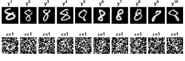
(a) original data samples and corresponding differentially private approximations using optimal noise adding mechanism ($\epsilon=1$)

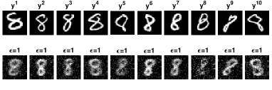
(b) original data samples and corresponding differentially private fabricated data samples ($\epsilon=1$)

Figure 1: An example of the data fabrication by means of a geometric model ensuring the geometric modeling error of fabricated data samples not to exceed that of original data samples without compromising on the value of privacy-loss bound $\epsilon$.

The central problem of this study is stated in the following:

Problem 1 (Central Problem).

To mitigate the accuracy-loss issue of differential privacy, the post-processing property of differential privacy is leveraged for fabricating new data samples by means of a geometric model ensuring the geometric modeling error of fabricated data samples not to be larger than that of original data samples while simultaneously achieving the privacy-loss bound.

Remark 1 (Motivation).

To our best knowledge, the state-of-the-art does not address Problem 1. It requires an approach to learn the representation of geometric structure induced by a finite set of data points. Encouraged by the fact that kernel-based solutions can be computed analytically and analyzed using a broad range of mathematical techniques, the approach opted in this study to address Problem 1 is of learning in Reproducing Kernel Hilbert Spaces (RKHS) the representation of data points to design a geometrically inspired model such that the model output range defines a bounded geometric structure in the affine hull of given data samples.

Kernels have been widely used in machine learning (?, ?) and can be scaled up for their applicability in large scale scenarios (?). Not only the parallels between the properties of deep neural networks and kernel methods have been established (?), but also deep kernel machines have been introduced (?, ?). Kernel autoencoders are effective models for representation learning. The kernel formulation of an autoencoder has been considered in (?) from a hashing perspective. A deep autoencoder, that aligns the latent code with a user-defined kernel matrix to learn similarity-preserving data representations, has been suggested (?). Further, a kernel autoencoder based on the composition of mappings from vector-valued reproducing kernel Hilbert spaces has been studied (?). Recently, a fuzzy theoretic approach to kernel based wide and conditionally deep autoencoders has been introduced (?, ?, ?, ?, ?, ?, ?, ?), wherein analytical solutions are derived for the learning of models using variational optimization technique. This approach has been further extended to privacy-preserving learning under a differential privacy framework (?, ?, ?). As an alternative to the SVM, the idea of affine hull large margin classifier has been investigated (?). Although kernel methods have been studied (?, ?, ?) under differential privacy, no previous study has considered geometrically inspired kernel methods to mitigate the accuracy-loss issue of differential privacy. State of the art lacks geometrically inspired kernel machines for scalable learning solutions that remain accurate even after providing differential privacy guarantee.

This study solves Problem 1 via making the following contributions (C1-C7):

Kernel Affine Hull Machines (C1):

For given distinct data points $(y^{i})_{i=1,\ldots,N}$ in some vector space we study the sets of the affine form rCl L & = {y = (w^1/∑_i=1^N w^i) y^1+ ⋯+ (w^N/∑_i=1^N w^i) y^N   ∣  w^i ∈R }, and ask for reasonable conditions on the real-valued scalars $(w^{i})_{i}$ to serve our purpose of representing the geometric structure induced by data points. First of all, in our approach $(w^{i})_{i}$ are considered to be functions in a RKHS. By postulating that indicator functions (specifically, their RKHS approximations) define scalar-valued functions $(w^{i})_{i}$, the set $\mathcal{L}$ actually can be identified by functions defining a subset in RKHS that represents our data points. This way we introduce the concept of Kernel Affine Hull Machine (KAHM) to learn kernel-based representation of multivariate scattered data as in the following:

Let $n,p,N$ be the positive integers and $\mathcal{X}\subset\mathbb{R}^{n}$ be a region. Let $\mathcal{H}_{k}(\mathcal{X})$ be the reproducing kernel Hilbert space of functions from $\mathcal{X}$ to $\mathbb{R}$ for a reproducing kernel $k:\mathcal{X}\times\mathcal{X}\rightarrow\mathbb{R}$. For a finite set of ordered pairs $\{(x^{i},y^{i})\in\mathcal{X}\times\mathbb{R}^{p}\;\mid\;i\in\{1,\cdots,N\}\}$ such that $\{x^{1},\cdots,x^{N}\}$ are pairwise distinct points, a point $y^{i}$ can be represented using indicator functions as rCl y^i & = 1_{x^1}(x^i)   y^1 + ⋯+ 1_{x^N}(x^i)  y^N, where $\mathbbm{1}_{\{x^{i}\}}$ is the indicator function of the set $\{x^{i}\}$. We approximate the indicator function $\mathbbm{1}_{\{x^{i}\}}$ through a function in $\mathcal{H}_{k}(\mathcal{X})$ that fits to the ordered pairs $\{\left(x^{j},\mathbbm{1}_{\{x^{i}\}}(x^{j})\right)\;\mid\;j\in\{1,\cdots,N\}\}$. The function in RKHS approximating $\mathbbm{1}_{\{x^{i}\}}$ is given as the solution of the following kernel regularized least squares problem: rCl h^i & = arg  min_f ∈H_k(X)   ( ∑_j=1^N |1_{x^i}(x^j) - f(x^j) |^2 + λ∥ f ∥^2_H_k(X) ),  λ∈R_+, where $\left\|f\right\|_{\mathcal{H}_{k}(\mathcal{X})}:=\sqrt{\left<f,f\right>_{\mathcal{H}_{k}(\mathcal{X})}}$ is the norm induced by the inner product on $\mathcal{H}_{k}(\mathcal{X})$. The fact that $h^{i}$ is an approximation of $\mathbbm{1}_{\{x^{i}\}}$ (i.e. the value $h^{i}(x)$ represents kernel-smoothed “membership” of $x$ to the set $\{x^{i}\}$) allows introducing a model based on the affine combination of $y^{1},\cdots,y^{N}$ as in the following: rCl A(x) & = h1(x)∑i=1Nhi(x) y^1 + ⋯+ hN(x)∑i=1Nhi(x)  y^N. Let $\mathrm{aff}(\{y^{1},\cdots,y^{N}\})$ denote the affine hull of $\{y^{1},\cdots,y^{N}\}$. The function $A:\mathcal{X}\rightarrow\mathrm{aff}(\{y^{1},\cdots,y^{N}\})$ is referred to as kernel affine hull machine, since it maps a point $x\in\mathcal{X}$ onto the affine hull of $\{y^{1},\cdots,y^{N}\}$ via learning representation of $x^{1},\cdots,x^{N}$ through functions in reproducing kernel Hilbert space. The image of $A$, rCCCl A[X] & := { A(x)   ∣  x ∈X } ⊂ aff({y^1,⋯,y^N }), defines a geometric structure in $\mathrm{aff}(\{y^{1},\cdots,y^{N}\})$. Fig. 2 displays a few examples of 3-dimensional samples and geometric structures defined by KAHMs’ images.

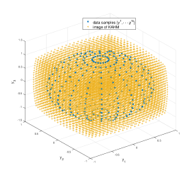
(a) first example

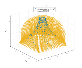
(b) second example

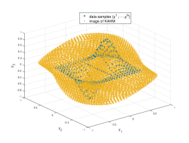
(c) third example

Figure 2: A few examples of 3-dimensional samples $\{y^{1},\cdots,y^{N}\}$ and geometric structures in $\mathrm{aff}(\{y^{1},\cdots,y^{N}\})$ defined by the images of corresponding KAHMs.

Regularization Parameter for Kernel Regularized Least Squares (C2):

Since indicator functions are approximated via solving a regularized least squares problem, the kernel regularized least squares problem is revisited in a deterministic setting with focus on the determination of regularization parameter. A reasonable choice for regularization parameter is to set it larger than the mean-squared-error on training samples. With this choice, the problem of determining regularization parameter can be reduced to an equivalent problem of finding the unique fixed point of a real-valued positive function. An iterative scheme, together with the mathematical proof of convergence, is provided to find the fixed point and thus to determine the regularization parameter.

Boundedness of KAHM and Distance Function (C3):

The KAHM mapping is a bounded function and thus the image of KAHM defines a bounded region in the affine hull of data samples. The boundedness of KAHM on data space is proven via deriving upper bounds on the Euclidean norm of KAHM output. The KAHM induces a function on data space, referred to as distance function, which is defined on a data point as equal to the distance between that point and its image under KAHM. The distance of an arbitrary point from its image (by the KAHM onto the affine hull of given data samples) is a measure of the distance between that arbitrary point and the given data samples. This is proven via deriving upper bounds on the ratio of these two distances.

KAHM Compositions for Data Representation Learning and Classification (C4):

The KAHM could serve as the building block for deep models. A nested composition of KAHMs, referred to as Conditionally Deep Kernel Affine Hull Machine, is considered for data representation learning. The conditionally deep KAHM discovers layers of increasingly abstract data representation with lowest-level data features being modeled by first layer and the highest-level by end layer. Further, a parallel composition of conditionally deep KAHMs, referred to as Wide Conditionally Deep Kernel Affine Hull Machine, is considered to efficiently learn the representation of big data. Similarly to the KAHM, both conditional deep KAHM and wide conditionally deep KAHM induce the distance function with value on a point indicating the distance of the point from data samples. This property of the distance function is leveraged to build a KAHM based classifier via modeling the region of each class through a separate KAHM based composition.

Membership-Inference Score for KAHM Based Classifier (C5):

Since the KAHM based classifier assigns a class-label to a data point based on the closeness of the point to the training data samples of that class, there is a possibility of an inference of the membership of a data point to the set of training data samples. To evaluate the potential of KAHM induced distance function in inferring the membership of a data point to the training dataset, a score, referred to as membership-inference score, is defined for evaluating the risk of membership inference attack. The membership-inference score is defined as the $L2$ distance between density of probability distribution on values of the distance function at training data points and the density of probability distribution on distance function values at test data points.

Differentially Private Data Fabrication for Classification (C6):

To ensure that KAHM based classifier keeps the privacy of training data protected, an optimal differentially private noise adding mechanism (?) is applied on training data samples. The noise added training data samples are smoothed through a transformation such that the error in KAHM modeling of smoothed data is not larger than the error in KAHM modeling of original data. It is shown that the error in KAHM modeling of smoothed data can be reduced to an arbitrary low value. The smoothed data samples, guaranteeing not only the differential privacy but also the geometric modeling error not to be larger than that of original data samples, serve as the fabricated data. The fabricated data samples are finally used to build the KAHM based differentially private classifier. The advantage of using fabricated data for classification is that fabricated data leads to a considerable reduction in the risk of membership inference attack with relatively much smaller loss of accuracy. Hence, the accuracy-loss issue of differential privacy is mitigated. Fig. 3 provides an example of differentially private classifier built with a 2-dimensional fabricated dataset with 3 classes.

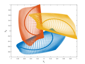
(a) data samples and images of corresponding KAHMs

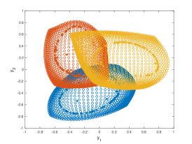
(b) differentially private fabricated data samples and images of corresponding KAHMs

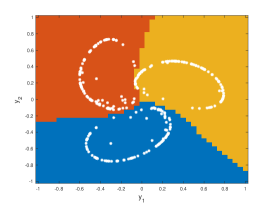
(c) decision boundaries determined by KAHM based differentially private classifier with fabricated data

Figure 3: An example of differentially private classifier built with a 2-dimensional fabricated dataset with 3 classes.

Application to Differentially Private Federated Learning (C7):

The different KAHMs built independently using different datasets can be combined together using the KAHM induced distance function. This allows introducing a federated learning scheme that combines together the local privacy-preserving KAHM based classifiers to build a global classifier. A significant feature of the scheme is that the evaluation of global classifier requires only locally computed distance measures.

The relation of the current study with previous works is confined to the following three points: 1) The wide and conditionally deep architecture consisting of the composition of kernel based models follows from (?, ?, ?, ?, ?), wherein a kernel based variational fuzzy model (motivated by measure theoretic basis (?)) is used. In contrast, the current study explores geometrically inspired kernel affine hull machines. 2) The input perturbation method (where noise is added to original data to achieve $(\epsilon,\delta)-$differential privacy of any subsequent computational algorithm) was earlier considered in (?, ?, ?). However, the current study complements the input perturbation method with a transformation to mitigate the accuracy-loss issue of differential privacy. 3) The current study follows the federated learning architecture of (?, ?, ?) with the difference that instead of fuzzy attributes, the KAHM induced distance measures are applied to aggregate the distributed local models for federated learning.

The significance and novelties of the contributions have been highlighted in Table 1 and Table 2 respectively.

Table 1: The significance of the contributions.

	Significance
C1	Representations learning in RKHS for defining a geometric structure in the affine hull of data samples
C2	Determination of the regularization parameter for kernel regularized least squares
C3	$\begin{array}[]{l}\mbox{Because of the boundedness of KAHM, the distance of an arbitrary point from its KAHM image}\\ \mbox{is a measure of the distance between that arbitrary point and the given data samples}\end{array}$
C4	$\begin{array}[]{l}\mbox{KAHM compositions learn geometrically inspired representations at varying abstraction level}\\ \mbox{facilitating classification via modeling the region of each class through a separate composition}\end{array}$
C5	Evaluation of the risk of membership inference attack on KAHM based classifier
C6	$\begin{array}[]{l}\mbox{Differentially private data fabrication to mitigate the accuracy-loss issue associated with}\\ \mbox{the differentially private classifier}\end{array}$
C7	Application to differentially private federated learning

Table 2: The novelties in the contributions.

	Novelty
C1	The concept of KAHM (Definition LABEL:def_affine_hull_model) is novel.
C2	$\begin{array}[]{l}\mbox{Determination of the regularization parameter as the unique fixed point of a}\\ \mbox{function (Theorem~{}\ref{result_definition_mse_function}) is novel.}\end{array}$
C3	$\begin{array}[]{l}\mbox{The idea of using bounded geometric structure (Theorem~{}\ref{result_kahm_bounded_function}) to define a measure of the distance}\\ \mbox{from given data samples (Theorem~{}\ref{result_ratio_distances}) is novel.}\end{array}$
C4	$\begin{array}[]{l}\mbox{Geometrically inspired representations learning at varying abstraction level and corresponding}\\ \mbox{induced measure of the distance from given data samples (Theorem~{}\ref{result_ratio_distances_cond_deep_KAHM}, Theorem~{}\ref{result_ratio_distances_wide_cond_deep_KAHM}) is novel.}\end{array}$
C5	$\begin{array}[]{l}\mbox{Quantification of membership inference attack risk as $L2$ distance between density of distance}\\ \mbox{from training data samples and density of distance from test data samples (Eq. (\ref{eq_270220231128})) is novel.}\end{array}$
C6	$\begin{array}[]{l}\mbox{Data fabrication via transforming differentially private data samples to reduce}\\ \mbox{geometric modeling error (Definition~{}\ref{def_transformation}, Theorem~{}\ref{result_transformation}, Definition~{}\ref{def_fabricated_data}) is novel.}\end{array}$
C7	$\begin{array}[]{l}\mbox{The feature of the federated learning that the evaluation of global classifier requires only}\\ \mbox{locally computed KAHM induced distance measures (Fig.~{}\ref{fig_KAHM_distributed_classifier}) is novel.}\end{array}$

The paper is organized into the following sections. The mathematical notation used throughout the paper is provided in Section 2. Section 3 introduces the concept of KAHM. KAHM based wide and deep models are presented in Section LABEL:sec_kahm_compositions for data representation learning. Differentially private classification application is considered in Section LABEL:sec_privacy followed by experimentation in Section LABEL:sec_experiments. Finally, the concluding remarks are presented in Section LABEL:sec_conclusion.

2 Notations

The following notations are introduced:

• Let $N,n,p,M,S,C\in\mathbb{Z}_{+}$ be the positive integers.

• Let $\mu_{max}(K)$ and $\mu_{min}(K)$ denote the maximum eigenvalue and minimum eigenvalue respectively of a square matrix $K$.

• Let $\sigma_{max}(K)$ and $\sigma_{min}(K)$ denote the maximum singular value and minimum singular value of a matrix $K$.

• Let $\mathrm{aff}(\mathbf{Y})$ denote the affine hull of a set $\mathbf{Y}\subset\mathbb{R}^{p}$.

• For a vector $y\in\mathbb{R}^{p}$, $\|y\|$ denotes the Euclidean norm of $y$.

• For a matrix $Y\in\mathbb{R}^{N\times p}$, $\|Y\|_{2}$ denotes the spectral norm, $\|Y\|_{F}$ denotes the Frobenius norm, $\|Y\|_{1}$ denotes the 1-norm, $\|Y\|_{\mathrm{max}}$ denotes the max norm, $(Y)_{i,:}$ denotes the $i-$th row, $(Y)_{:,j}$ denotes the $j-$th column, and $(Y)_{i,j}$ denotes the $(i,j)-$th element of $Y$.

• Let $\circ$ denote the Hadamard product.

• Let $I_{N}$ denote the identity matrix of the size $N$ and $\mathbf{1}_{N}$ denotes the $N\times 1$ vector of ones.

• Let $\mathbbm{1}_{\mathbf{Y}}$ denote the indicator function of the set $\mathbf{Y}$.

• Let $\mathcal{X}\subset\mathbb{R}^{n}$ be a region.

• $K\succ 0$ denotes that a symmetric matrix $K$ is positive definite.

• A Reproducing Kernel Hilbert Space (RKHS), $\mathcal{H}_{k}(\mathcal{X})$, is a Hilbert space of functions $f:\mathcal{X}\rightarrow\mathbb{R}$ on a non-empty set $\mathcal{X}$ with a reproducing kernel $k:\mathcal{X}\times\mathcal{X}\rightarrow\mathbb{R}$ satisfying $\forall x\in\mathcal{X}$ and $\forall f\in\mathcal{H}$,

  • $k(\cdot,x)\in\mathcal{H}_{k}(\mathcal{X})$,

  • $\left<f,k(\cdot,x)\right>_{\mathcal{H}_{k}(\mathcal{X})}=f(x)$,

  where $\left<\cdot,\cdot\right>_{\mathcal{H}_{k}(\mathcal{X})}:\mathcal{H}_{k}(\mathcal{X})\times\mathcal{H}_{k}(\mathcal{X})\rightarrow\mathbb{R}$ is an inner product on $\mathcal{H}_{k}(\mathcal{X})$.

• Let $\left\|f\right\|_{\mathcal{H}_{k}(\mathcal{X})}:=\sqrt{\left<f,f\right>_{\mathcal{H}_{k}(\mathcal{X})}}$ denote the norm induced by the inner product on $\mathcal{H}_{k}(\mathcal{X})$.

3 Kernel Affine Hull Machines

The computation of KAHM requires solving a kernel regularized least squares problem. Therefore the kernel regularized problem is revisited (in Section 3.1) with focus on the determination of regularization parameter (in Section LABEL:sec_regularization_parameter). The obtained solution is applied (in Section LABEL:sec_learning_representation) to learn data representation in RKHS facilitating the definition of KAHM (in Section LABEL:sec_an_affine_hull_machine).

3.1 Kernel Regularized Least Squares

Given a training data set $\left\{(x^{i},y^{i})\in\mathcal{X}\times\mathbb{R}^{p}\;\mid\;i\in\{1,\cdots,N\}\right\}$ such that $\{x^{1},\cdots,x^{N}\}$ are pairwise distinct points, consider a positive-definite real-valued kernel $k:\mathcal{X}\times\mathcal{X}\rightarrow\mathbb{R}$ on $\mathcal{X}$ with a corresponding RKHS $\mathcal{H}_{k}(\mathcal{X})$. Assuming that $\mathcal{X}\subset\mathbb{R}^{n}$, real-valued matrices $X\in\mathbb{R}^{N\times n}$ and $Y\in\mathbb{R}^{N\times p}$ are defined as rCl X & = [[][c],c/c/c, x^1 ⋯ x^N ]^T
Y = [[][c],c/c/c, y^1 ⋯ y^N ]^T. Let $(Y)_{:,j}$ denote the $j-$th column of $Y$, i.e., rCl (Y)_:,j & = [[][c],c/c/c, y^1_j ⋯ y^N_j ]^T, where $j\in\{1,\cdots,p\}$ and $y^{i}_{j}$ is the $j-$th element of $i-$th output sample $y^{i}$. The solution of the following regularized least squares problem: rCl f^*_k,X,(Y)_:,j,λ & = arg  min_f ∈H_k(X)   ( ∑_i=1^N |y^i_j - f(x^i) |^2 + λ∥ f ∥^2_H_k(X) ),  λ∈R_+, using the representer theorem (?), can be written as rCl f^*_k,X,(Y)_:,j,λ(x) & = [[][c],c/c/c, k(x,x^1) ⋯ k(x,x^N) ] (K_X + λI_N )^-1 (Y)