Abstract

We use the PyNeb 1.1.16 Python package to evaluate the atomic datasets available for the spectral modeling of [Fe ii] and [Fe iii], which list level energies, $A$-values, and effective collision strengths. Most datasets are reconstructed from the sources, and new ones are incorporated to be compared with observed and measured benchmarks. For [Fe iii], we arrive at conclusive results that allow us to select the default datasets, while for [Fe ii], the conspicuous temperature dependency on the collisional data becomes a deterrent. This dependency is mainly due to the singularly low critical density of the $\mathrm{3d^{7}\ a\,^{4}F_{9/2}}$ metastable level that strongly depends on both the radiative and collisional data, although the level populating by fluorescence pumping from the stellar continuum cannot be ruled out. A new version of PyNeb (1.1.17) is released containing the evaluated datasets.

1 1 0 Academic Editor: Alexander Kramida 6 February 2023 14 March 2023 23 March 2023 https://doi.org/ Atomic Data Assessment with PyNeb: Radiative and Electron Impact Excitation Rates for [Fe ii] and [Fe iii] Atomic Data Assessment with PyNeb: Radiative and Electron Impact Excitation Rates for [Fe ii] and [Fe iii] Claudio Mendoza ^1,*, José E. Méndez-Delgado ², Manuel Bautista ³, Jorge García-Rojas ^4,5 and Christophe Morisset ⁶ Claudio Mendoza, José E. Méndez-Delgado, Manuel Bautista, Jorge García-Rojas and Christophe Morisset Mendoza, C.; Méndez-Delgado, J. E.; Bautista, M.; García-Rojas, J.; Morisset, C. Correspondence: claudiom07@gmail.com; Tel.: +1-269-370-8465

1 Introduction

PyNebhttp://research.iac.es/proyecto/PyNeb/ Luridiana et al. (2012, 2015) is a widely used Python tool for the analysis of emission lines in nebular plasmas to determine the temperature, density, and chemical abundances Peimbert et al. (2017). It essentially solves the equations of statistical equilibrium by addressing an extensive atomic database of radiative and collisional rates; therefore, PyNeb’s diagnostic potential relies directly on the accuracy of this database. In this respect, its data curation strategy is based on the selection of recommended default datasets and keeping access to a historical archive of radiative and collisional files rather than discarding them. This singular scheme allows modelers to estimate the uncertainties of the plasma diagnostics and chemical abundances due to the scatter of the atomic parameters. It also provides a versatile environment for atomic data assessment, which has been previously used productively to benchmark the accuracy of the radiative rates in N- and P-like ions and effective collision strengths in C-like ions Morisset et al. (2020) and to determine the atomic-data impact on density diagnostics Juan de Dios and Rodríguez (2021).

As a follow-up to Morisset et al. (2020), we apply PyNeb’s capabilities to assess the radiative and collisional rates associated with the transition arrays of [Fe ii] and [Fe iii]. These ions give rise to forbidden lines in the optical and infrared spectra of H ii regions, planetary nebulae, and quasars that are used to determine plasma conditions and iron abundance, the latter particularly in the context of depletion factors in the life cycle of dust grains Perinotto et al. (1999); Delgado Inglada et al. (2009); Delgado-Inglada et al. (2016). These iron transition arrays are also useful for studying the shocked plasma caused by outflows from newborn stars that form bright Herbig–Haro (HH) objects perturbing stellar accretion Mesa-Delgado et al. (2009); Méndez-Delgado et al. (2021a, b). The high-resolution spectra of such HH objects—e.g., HH 202S Mesa-Delgado et al. (2009) and HH 204 Méndez-Delgado et al. (2021b) in the Orion Nebula—taken with the Ultraviolet Visual Echelle Spectrograph (range 3100–10,400 Å) D’Odorico et al. (2000) present an observational opportunity to benchmark the Fe ii and Fe iii atomic data. The optical emission spectra of these two HH objects are dominated by photoionization from $\theta^{1}$ Ori C, the main ionization source of the Orion Nebula, and can therefore be treated as small-scale H ii regions Méndez-Delgado et al. (2021a).

Due to the astrophysical importance of Fe ii, the computation of radiative and collisional rates for the spectral modeling of this system has received considerable attention since the early semi-empirical computations of $A$-values (radiative transition probabilities) for the forbidden Garstang (1962) and dipole-allowed Kurucz and Peytremann (1975) transitions and electron-impact collision strengths with the distorted wave method Nussbaumer and Storey (1980); Nussbaumer et al. (1981). Our intention here is not to evaluate this vast body of data but to concentrate on complete and accurate datasets to model the spectra of [Fe ii] and [Fe iii] observed in nebular plasmas.

A landmark systematic effort to compute radiative and collisional data for the fine-structure spectral modeling of Fe ions was undertaken by the Iron Projecthttp://cdsweb.u-strasbg.fr/topbase/testop/TheIP.html using the $R$-matrix method Hummer et al. (1993) and relativistic multi-configuration structure codes such as superstructure Eissner et al. (1974), civ3 Hibbert (1975), and hfr  Cowan (1981). For Fe ii and Fe iii, $A$-values were computed for both allowed and forbidden lines Nahar (1995); Nahar and Pradhan (1996); Quinet et al. (1996) and electron-impact effective collision strengths (ECS) for infrared, optical, and ultraviolet transitions Zhang and Pradhan (1995); Zhang (1996); Bautista and Pradhan (1996). Although these $R$-matrix calculations were originally performed in $LS$ coupling followed by algebraic transformations to intermediate coupling, more recent scattering calculations for these ionic species Bautista et al. (2010); Badnell and Ballance (2014); Bautista et al. (2015); Tayal and Zatsarinny (2018); Smyth et al. (2019) have relied on $R$-matrix implementations based on the Breit–Pauli Hamiltonian (bprm Berrington et al. (1995), bsr Zatsarinny (2006)) and Dirac–Fock Hamiltonian (darc Ait-Tahar et al. (1996)). In some cases, e.g., the collisional excitation of levels within the Fe⁺ ground configuration, low-temperature ECS have been computed with several $R$-matrix implementations—intermediate coupling frame transformation (icft, Griffin et al. (1998)), bprm, and darc—to obtain uncertainty estimates Wan et al. (2019).

Extensive multi-configuration Breit–Pauli (mcbp) calculations of $gf$-values (weighted oscillator strengths) and $A$-values for allowed and forbidden transitions in Fe ii and Fe iii Deb and Hibbert (2008, 2009a, 2009b, 2010a, 2010b, 2011, 2014) with the code civ3 have shown that fine-tuning corrections to the Hamiltonian matrix by fitting to the experimental level energies lead to more accurate configuration expansions. However, significant $A$-value differences (greater than 20–30%) are found for some transitions computed with comparable multi-configuration methods that also implement fine-tuning corrections (e.g., Quinet (1996); Quinet et al. (1996); Fivet et al. (2016)), which are caused by strong configuration mixing, double-excitation representations, and subtle core–valence correlation involving the closed 3p⁶ and open 3dⁿ subshells.

Since the Fe ii radiative data display a large scatter, experimentalists and astronomical observers have been enticed to measure accurate radiative parameters such as lifetimes and branching fractions to determine $A$- and $gf$-values; however, most of them address allowed transitions involving odd-parity states. Lifetimes have been measured for 21 Fe ii levels with a time-resolved nonlinear laser-induced fluorescence technique to an accuracy of 2–3%, and by means of branching fractions, absolute $A$-values were reported to be within 6% and 26% for the strong and weak transitions, respectively Schnabel et al. (2004). Accurate $gf$-values for 142 Fe ii lines were determined from laboratory and solar spectroscopic multiplets and theoretical fine-structure ratios, assuring that oscillator-strength error no longer hinders stellar abundance studies Meléndez and Barbuy (2009). Branching fractions have been measured for 121 ultraviolet Fe ii lines (2250–3280 Å), and through published lifetimes, $gf$-values have been derived and applied to iron abundance determinations in the Sun and the metal-poor star HD 84937 Den Hartog et al. (2019). Good agreement is obtained with the Fe standard solar abundance. On the other hand, the only lifetime measurements of [Fe ii] even-parity metastable states to derive transition probabilities have been carried out by the Ferrum Project using a laser probing technique on a stored ion beam, the branching fractions being derived from astrophysical spectra Rostohar et al. (2001); Hartman et al. (2003); Gurell et al. (2009). Consistent differences between the observed intensity ratios and theoretical branching fractions have suggested that the [Fe ii] lines might be used to determine reddening.

In the present data assessment, we revise the Fe ii and Fe iii atomic datasets—namely, energy levels, $A$-values, and ECS—available in PyNeb 1.1.16. In most cases, we reconstruct the atomic models from the sources by mapping the rates to the NIST level structure. We renormalize the number of levels to a predefined value to enable one-to-one comparisons among the theoretical datasets and benchmarks with the HH 202S and HH 204 spectra and the aforementioned experimental data. We also extend the PyNeb database with additional new datasets, the main objective being the default selection for a new version: PyNeb 1.1.17.

We give a brief description of PyNeb’s file structure and methods in Section 2, and carry out the data assessments and discussions of Fe iii and Fe ii in Sections 3 and 4 followed by the conclusions in Section 5.

2 PyNeb

A brief description of the PyNeb package is given in Morisset et al. (2020), in particular of its object-oriented architecture. The ion object is thereby represented by the Atom class, offering a set of methods through the atomicData manager. Regarding energy levels, $A$-values, and ECS, PyNeb has three file types:

• $xxx\_$levels.dat: lists NIST energy levels for ionic species $xxx$;

• $xxx\_$atom_ref.dat: lists $A$-values for transitions between energy levels of ion $xxx$ contained in the ref dataset;

• $xxx\_$coll_ref.dat: lists ECS for transitions between energy levels of ion $xxx$ contained in the ref dataset.

A printout of the NIST energy levels for a specific ion, Fe iii say, may be obtained with the function getLevelsNIST():

     # Call thePyNeb Python module  import pyneb as pn  # List NIST energy levels for Fe III  levels = pn.getLevelsNIST(’Fe3’)  print(levels)     and a list of all the Fe iii atom and coll files is currently available with:

     pn.atomicData.getAllAvailableFiles(’Fe3’)     

[’* fe_iii_atom_Q96_J00.dat’, ’* fe_iii_coll_Z96.dat’, ’fe_iii_atom_BBQ10.dat’, ’fe_iii_atom_NP96.dat’, ’fe_iii_coll_BB14.dat’, ’fe_iii_coll_BBQ10.dat’]where the recommended default files are prefixed with an asterisk. Alternative files may be easily accessed by the user to replace the default files with the function

     pn.atomicData.setDataFile(’fe_iii_atom_BBQ10.dat’)  pn.atomicData.setDataFile(’fe_iii_coll_BBQ10.dat’)     

We can now instantiate the Fe iii ion with the new atomic datasets

     pn.atomicData.getDataFile(’Fe3’)  Fe3=pn.Atom(’Fe’,3,NLevels=34)     and apply a series of methods to determine some of its plasma properties:

     # Emissivity for transition 2-1 at T = 1.0e4 K and n_e = 1.0e4 cm-3  Fe3.getEmissivity(tem=1.0e4,den=1.0e4,lev_i=2,lev_j=1)  # Emissivity for transition with wavelength 4658.17 A at T = 1.0e4 K  # and n_e = 1.0e4 cm-3  Fe3.getEmissivity(tem=1.0e4,den=1.0e4,wave=4658.17)  # Level critical densities at T = 1.0e4 K  Fe3.getCritDensity(1.0e4)  # Level populations at T = 1.0e4 K and n_e = 1.0e4 cm-3  Fe3.getPopulations(tem=1.0e4, den=1.0e4)     In the ion instantiating command above, the option NLevels specifies the number of levels of the atomic model, which can be the total (default) or a reduced set.

A complete list of methods is included in the PyNeb manual. The Atom class also addresses the ion atomic properties, e.g., the ECS at a selected temperature

     # Collision strength for transition 2-1 at T = 1.0e4 K  Fe3.getOmega(1.0e4,2,1)     This function is useful as it returns the interpolated value at the prescribed input temperature allowing comparisons between different ECS datasets with tabulations on diverse temperature ranges. The original temperature and ECS arrays may be listed with the commands

     # Temperature and collision strength original arrays  Fe3.getTemArray()  Fe3.getOmegaArray()     

3 Fe iii

3.1 Fe iii Atomic Datasets in PyNeb

Fe iii atomic models in PyNeb 1.1.16 comprise 34 fine-structure levels (energy $E<60,000$ cm^-1) from the $\mathrm{3d^{6}}$ and $\mathrm{3d^{5}4s}$ electron configurations, whose attributes were obtained from the NIST server (April 2017). Levels $\mathrm{3d^{6}}$ $\mathrm{b\,^{1}D_{2}}$ and $\mathrm{b\,^{1}S_{0}}$ at $E>77,000$ cm^-1 are therefore not taken into account, and from the $\mathrm{3d^{5}4s}$ configuration, only the lowly lying $\mathrm{{}^{7}S_{3}}$ and $\mathrm{{}^{5}S_{2}}$ are included. Transitions among the levels of these two even-parity configurations are electric dipole (E1) forbidden and thus occur via electric quadrupole (E2) and magnetic dipole (M1) operators. Shortcomings in the spectral fits resulting from the number of levels in the atomic models, 34 levels in this case, will be examined by comparing with extended models of 144 levels (see Section 3.2).

Two fundamental interactions in the computation of accurate radiative ($A$-values) and collisional (ECS) rates for atomic ions are electron correlation (configuration interaction, CI) and relativistic coupling. We give below brief descriptions of the numerical methods and approximations that were used to compute the datasets available in PyNeb 1.1.16.

atom_NP96

—Contains $A$-values for E2 and M1 transitions computed in an extensive CI framework with the multi-configuration Breit–Pauli (mcbp) code superstructure Nahar and Pradhan (1996).

coll_Z96

—ECS were calculated in an 83-term non-relativistic $R$-matrix calculation including the $\mathrm{3d^{6}}$, $\mathrm{3d^{5}4s}$, and $\mathrm{3d^{5}4p}$ configurations. ECS for 219 fine-structure levels were then obtained through algebraic recoupling Zhang (1996).

atom_Q96_J00

—The Pauli Hartree–Fock hfr code was used to compute $A$-values for the radiative transitions within the $\mathrm{3d^{6}}$ configuration Quinet (1996). Wave functions were generated with CI expansions adjusting the electrostatic and spin–orbit integrals to fit the spectroscopic level energies. $A$-values for the $\mathrm{3d^{5}4s\ ^{7}S_{3}}$ and $\mathrm{{}^{5}S_{2}}$ levels were obtained independently with hfr using empirically adjusted Slater parameters Johansson et al. (2000).

atom_BBQ10, coll_BBQ10

—A 36-configuration CI expansion including pseudo-orbitals ($\overline{4f}$, $\overline{5s}$, $\overline{5p}$, and $\overline{5d}$) was used to compute $A$-values with the mcbp autostructure atomic structure code Bautista et al. (2010); Badnell (2011). Term-energy corrections were introduced to fine-tune the wave functions. ECS were computed with the Dirac–Coulomb $R$-matrix package (darc) based on a 3-configuration target constructed with the grasp92 multi-configuration Dirac–Hartree–Fock structure code Parpia et al. (1996) under the extended average level approximation.

coll_BB14

—ECS were computed with the icft $R$-matrix method using a 136-term (322 fine-structure levels) target representation Badnell and Ballance (2014). This mcbp 3-configuration target was generated with autostructure using a Thomas–Fermi–Dirac–Amaldi model potential.

3.2 Fe iii Revised and New Atomic Datasets

The present work intends to revise the datasets currently available in PyNeb, incorporate new ones, and implement procedures for data evaluation. For such purposes, we have collected the data from the original sources, verified consistency, and implemented new atom and coll files. To begin with, we have introduced a new level file, fe_iii_levels.dat, with updated spectroscopic measurements (improved accuracy and new levels such as $\mathrm{3d^{6}\ b\,^{1}D_{2}}$) from the NIST database (July 2022) Kramida et al. (2021). We list below the revised and new atomic datasets with brief descriptions; the suffix “$\_n$” is now appended to the dataset label, where $n$ is the number of levels in the atomic model. For data comparisons, we have normalized all Fe iii datasets to 34 levels, but to estimate model convergence, we have extended some models to 144 levels.

An important issue is how to deal with missing energy levels in both the theoretical and spectroscopic reports since the PyNeb energy-level files are based on the NIST database, which is incomplete at the higher energies. In spectrum modeling, levels with zero decay rates may lead to numerical problems; we have, therefore, limited the number of levels in the atomic models to those that have been both computed and measured. From the user’s point of view, modeling turnaround time is also an important issue; therefore, the number of levels in the atomic models must take this point into consideration.

atom_Q96_34

—The main differences with the atom_Q96_J00 dataset described in Section 3.1 are the $A$-values for transitions involving the $\mathrm{3d^{5}4s\ ^{7}S_{3}}$ and $\mathrm{{}^{5}S_{2}}$ levels. The radiative rates in atom_Q96_J00 for transitions decaying from the $\mathrm{{}^{7}S_{3}}$ upper level are set to $A=0.0$, while those from $\mathrm{{}^{5}S_{2}}$ were calculated with hfr with empirically adjusted Slater parameters Johansson et al. (2000). In this dataset, radiative rates for transitions involving these levels have been updated with $A$-values from atom_BB14_34. This choice is to a certain extent arbitrary as inferred from the wide $A$-value scatter shown for the transitions $\mathrm{{}^{5}S_{2}}-\mathrm{{}^{5}D}_{J}$ in Table 1. We include in this comparison $A$-values computed with extensive CI using both hfr and autostructure (atom_FBQh16 and atom_FBQa16) Fivet et al. (2016); however, these datasets lack the completeness required to model collisionally excited nebular lines and, consequently, will not be further considered in the present data assessment.

Table 1: $A$-value comparison for the $\mathrm{3d^{5}4s\ ^{5}S_{2}}-\mathrm{3d^{6}\ {}^{5}D}_{J}$ transitions in [Fe iii]. $A$-values in J00 were calculated with the semi-relativistic hfr code using empirical Slater parameters Johansson et al. (2000) and included in the atom_Q96_J00 dataset (see Section 3.1). The methods used to compute the radiative data in atom_BBQ10_34 and atom_BB14_34 are described below. $A$-values in atom_FBQh16 and atom_FBQa16 were, respectively, computed with hfr and autostructure with extensive CI Fivet et al. (2016).

$J$	$\lambda_{\mathrm{air}}$ (Å)	$A$-Value (s-1)
		J00	BBQ10_34	BB14_34	FBQh16	FBQa16
4	2438.28	22.2	25.7	38.4	32.0	31.6
3	2464.48	16.0	18.7	28.0	23.3	23.1
2	2483.01	11.0	12.8	19.1	15.9	15.8
1	2495.01	6.4	7.43	11.1	9.29	9.22
0	2500.93	2.0	2.44	3.66

coll_Z96_34

—ECS listed in the supplementary data associated with the original publication Zhang (1996) were downloaded directly from the CDS to build a new file (see Section 3.1 for details of the calculation).

coll_Z96_144

—The coll_Z96_34 dataset was extended to include 144 levels from the $\mathrm{3d^{6}}$, $\mathrm{3d^{5}4s}$, and $\mathrm{3d^{5}4p}$ configurations with $E<121,500$ cm^-1. For higher energies, inconsistencies in the reported list of measured and computed levels begin to appear. Although this model extension is not expected to contribute to the collisionally excited nebular lines, it may be relevant if the populations of the $\mathrm{3d^{5}4p}$ levels generate E1 arrays.

atom_DH09_34

—$A$-values for the E2 and M1 transitions between levels of the $\mathrm{3d^{6}}$ configuration have been computed with the mcbp code civ3 Hibbert (1975); Hibbert et al. (1991) in a CI scheme spanning single and double excitations Deb and Hibbert (2009a). To improve accuracy, the diagonal elements of the Hamiltonian matrix were fine-tuned to fit the experimental energies. Similarly to atom_Q96_34, $A$-values for transitions involving the $\mathrm{3d^{5}4s\ ^{7}S_{3}}$ and $\mathrm{{}^{5}S_{2}}$ levels are taken from atom_BB14_34.

atom_BBQ10_34, coll_BBQ10_34

—$A$-values and ECS were downloaded from the xstar database Mendoza et al. (2021), and the PyNeb atom and coll files were rebuilt.

atom_BB14_34, coll_BB14_34

—Computed $A$-values and ECS were obtained from the
crlike_nrb13#fe2.dat adf04 file downloaded from the open-adashttps://open.adas.ac.uk/ database. Details of the ECS computation Badnell and Ballance (2014) are described in Section 3.1. No information is given in the adf04 file on the provenance of the radiative data; thus, we assume they are coproducts of the target calculation.

atom_BB14_144, coll_BB14_144

—The BB14_34 model has been extended to include 144 levels from the $\mathrm{3d^{6}}$, $\mathrm{3d^{5}4s}$, and $\mathrm{3d^{5}4p}$ configurations with $E<121,500$ cm^-1.

3.3 Fe iii Observational Benchmarks

3.3.1 $A$-Value Ratio Benchmark

It is well known that the intensity ratio of two spectral lines arising from a common upper level can be expressed as

$$\frac{I(j,i)}{I(j,i^{\prime})}=\frac{A(j,i)}{A(j,i^{\prime})}\times\frac{\lambda(j,i^{\prime})}{\lambda(j,i)}$$ (1)

enabling an observational benchmark of the theoretical $A$-value ratio $A(j,i)/A(j,i^{\prime})$. This measure provides indications of the accuracy of both the observed intensities and computed radiative rates, signposting unreliable lines to be excluded from the spectrum fits.

In Tables 2 and 3, we compare the observed line-intensity ratios from HH 202S and HH 204  Mesa-Delgado et al. (2009); Méndez-Delgado et al. (2021b) with the $A$-value ratios from the BBQ10_34, BB14_34, DH09_34, and Q96_34 atom files. The relative uncertainties in the observed intensity ratios from HH 202S are, in general, larger than those from HH 204. Although both spectra are of comparable quality, HH 204 was observed under photometric conditions whereby the absolute calibration error is slightly smaller; moreover, the HH 204 integrated emission comprised twice the area of HH 202S with longer exposure times.

For both sources, the observed intensity ratios for transitions arising from levels $\mathrm{3d^{6}\ a\,^{3}F}_{J}$ or lower and ending up at a level within the ground configuration $\mathrm{3d^{6}\ a\,^{5}D}$ with wavelengths $\lambda>4600$ Å are generally more accurate (better than 15%). For transitions arising from higher levels, uncertainties as large as 70% have been listed. On the other hand, most theoretical ratios agree to within 10% except for significantly discrepant cases in atom_BBQ10_34: $I(\lambda 3286)/I(\lambda 8729)$; $I(\lambda 3366)/I(\lambda 9960)$; and $I(\lambda 3357)/I(\lambda 8838)$. As a whole, the theoretical ratios lie within the observed ratio error bars except for some questionable lines in HH 202S ($\lambda 8729$, affected by telluric absorptions) and in HH 204 ($\lambda\lambda 4080,4097$ blended with O ii lines and $\lambda\lambda 7078,7088,9204$ being misidentifications).

Table 2: Comparison of observed [Fe iii] line intensity ratios in HH 202S (Obs) for transitions sharing a common upper level with those estimated from the $A$-values in the BBQ10_34, BB14_34, DH09_34, and Q96_34 atom files. The error of the least significant figure of the observed intensity ratio is indicated in brackets.

Line 1			Line 2		Obs	BBQ10_34	BB14_34	DH09_34	Q96_34
Upper	Lower	$\lambda_{\mathrm{air}}$(Å)	Lower	$\lambda_{\mathrm{air}}$(Å)	Line Intensity Ratio
$\mathrm{3d^{6}\ {}^{3}D_{3}}$	$\mathrm{3d^{6}\ {}^{5}D_{4}}$	3239.79	$\mathrm{3d^{6}\ {}^{5}D_{3}}$	3286.24	4(1)	3.58	3.59	3.28	3.60
$\mathrm{3d^{6}\ {}^{3}D_{3}}$	$\mathrm{3d^{6}\ {}^{5}D_{3}}$	3286.24	$\mathrm{3d^{6}\ a\,^{3}P_{2}}$	8728.84	2.0(5)	4.88	3.12	3.80	3.29
$\mathrm{3d^{6}\ {}^{3}D_{1}}$	$\mathrm{3d^{6}\ {}^{5}D_{1}}$	3355.50	$\mathrm{3d^{6}\ {}^{5}D_{0}}$	3366.22	1.6(8)	1.13	1.12	1.16	1.14
$\mathrm{3d^{6}\ {}^{3}D_{1}}$	$\mathrm{3d^{6}\ {}^{5}D_{0}}$	3366.22	$\mathrm{3d^{6}\ a\,^{3}P_{1}}$	9959.85	5(4)	9.07	5.42	6.37	5.54
$\mathrm{3d^{6}\ {}^{3}D_{2}}$	$\mathrm{3d^{6}\ {}^{5}D_{2}}$	3334.95	$\mathrm{3d^{6}\ {}^{5}D_{1}}$	3356.59	1.2(2)	1.14	1.15	1.20	1.18
$\mathrm{3d^{6}\ {}^{3}D_{2}}$	$\mathrm{3d^{6}\ {}^{5}D_{1}}$	3356.59	$\mathrm{3d^{6}\ a\,^{3}P_{2}}$	8838.14	4.1(8)	6.01	4.28	4.39	4.19
$\mathrm{3d^{5}4s\ ^{7}S_{3}}$	$\mathrm{3d^{6}\ {}^{5}D_{4}}$	3322.47	$\mathrm{3d^{6}\ {}^{5}D_{3}}$	3371.35	1.4(3)	1.38	1.37
$\mathrm{3d^{5}4s\ ^{7}S_{3}}$	$\mathrm{3d^{6}\ {}^{5}D_{3}}$	3371.35	$\mathrm{3d^{6}\ {}^{5}D_{2}}$	3406.11	2.2(5)	2.33	2.31
$\mathrm{3d^{6}\ {}^{3}G_{3}}$	$\mathrm{3d^{6}\ {}^{5}D_{3}}$	4046.49	$\mathrm{3d^{6}\ {}^{5}D_{2}}$	4096.68	2.3(8)	2.27	2.45	2.56	2.53
$\mathrm{3d^{6}\ {}^{3}G_{4}}$	$\mathrm{3d^{6}\ {}^{5}D_{4}}$	4008.34	$\mathrm{3d^{6}\ {}^{5}D_{3}}$	4079.69	3.8(7)	3.15	3.63	3.62	3.92
$\mathrm{3d^{6}\ a\,^{3}F_{2}}$	$\mathrm{3d^{6}\ {}^{5}D_{3}}$	4667.11	$\mathrm{3d^{6}\ {}^{5}D_{2}}$	4734.00	0.29(4)	0.28	0.28	0.29	0.28
$\mathrm{3d^{6}\ a\,^{3}F_{2}}$	$\mathrm{3d^{6}\ {}^{5}D_{2}}$	4734.00	$\mathrm{3d^{6}\ {}^{5}D_{1}}$	4777.70	2.0(3)	2.06	2.07	2.09	2.08
$\mathrm{3d^{6}\ a\,^{3}F_{3}}$	$\mathrm{3d^{6}\ {}^{5}D_{4}}$	4607.12	$\mathrm{3d^{6}\ {}^{5}D_{3}}$	4701.64	0.19(3)	0.18	0.18	0.19	0.17
$\mathrm{3d^{6}\ a\,^{3}F_{3}}$	$\mathrm{3d^{6}\ {}^{5}D_{3}}$	4701.64	$\mathrm{3d^{6}\ {}^{5}D_{2}}$	4769.53	2.8(3)	2.89	2.90	2.93	2.94
$\mathrm{3d^{6}\ a\,^{3}F_{4}}$	$\mathrm{3d^{6}\ {}^{5}D_{4}}$	4658.17	$\mathrm{3d^{6}\ {}^{5}D_{3}}$	4754.81	5.3(6)	5.28	5.40	5.32	5.49
$\mathrm{3d^{6}\ a\,^{3}P_{1}}$	$\mathrm{3d^{6}\ {}^{5}D_{2}}$	5011.41	$\mathrm{3d^{6}\ {}^{5}D_{0}}$	5084.85	5.9(9)	5.72	6.12	5.97	5.95
$\mathrm{3d^{6}\ {}^{3}H_{4}}$	$\mathrm{3d^{6}\ {}^{5}D_{4}}$	4881.07	$\mathrm{3d^{6}\ {}^{5}D_{3}}$	4987.29	5.4(7)	4.99	5.33	5.50	5.76
$\mathrm{3d^{6}\ a\,^{3}P_{2}}$	$\mathrm{3d^{6}\ {}^{5}D_{3}}$	5270.57	$\mathrm{3d^{6}\ {}^{5}D_{1}}$	5412.06	11(2)	10.2	11.4	11.4	11.0

Table 3: Comparison of observed [Fe iii] line intensity ratios in HH 204 (Obs) for transitions sharing a common upper level with those estimated from $A$-values in the BBQ10_34, BB14_34, DH09_34, and Q96_34 atom files. The error of the least significant figure of the observed intensity ratio is indicated in brackets.

Line 1			Line 2		Obs	BBQ10_34	BB14_34	DH09_34	Q96_34
Upper	Lower	$\lambda_{\mathrm{air}}$(Å)	Lower	$\lambda_{\mathrm{air}}$(Å)	Line Intensity Ratio
$\mathrm{3d^{6}\ {}^{3}D_{3}}$	$\mathrm{3d^{6}\ {}^{5}D_{4}}$	3239.79	$\mathrm{3d^{6}\ {}^{5}D_{3}}$	3286.24	3.6(9)	3.58	3.59	3.28	3.60
$\mathrm{3d^{6}\ {}^{3}D_{3}}$	$\mathrm{3d^{6}\ {}^{5}D_{3}}$	3286.24	$\mathrm{3d^{6}\ {}^{5}D_{2}}$	3319.27	1.0(4)	1.35	1.36	1.47	1.41
$\mathrm{3d^{6}\ {}^{3}D_{3}}$	$\mathrm{3d^{6}\ {}^{5}D_{2}}$	3319.27	$\mathrm{3d^{6}\ a\,^{3}P_{2}}$	8728.84	3.1(8)	3.62	2.30	2.59	2.35
$\mathrm{3d^{6}\ {}^{3}D_{1}}$	$\mathrm{3d^{6}\ {}^{5}D_{1}}$	3355.50	$\mathrm{3d^{6}\ {}^{5}D_{0}}$	3366.22	1.5(3)	1.13	1.12	1.16	1.14
$\mathrm{3d^{6}\ {}^{3}D_{2}}$	$\mathrm{3d^{6}\ {}^{5}D_{2}}$	3334.95	$\mathrm{3d^{6}\ {}^{5}D_{1}}$	3356.59	1.2(3)	1.14	1.15	1.20	1.18
$\mathrm{3d^{6}\ {}^{3}D_{2}}$	$\mathrm{3d^{6}\ {}^{5}D_{1}}$	3356.59	$\mathrm{3d^{6}\ a\,^{3}P_{2}}$	8838.14	5.3(7)	6.01	4.28	4.39	4.19
$\mathrm{3d^{6}\ {}^{1}I_{6}}$	$\mathrm{3d^{6}\ {}^{3}H_{6}}$	9701.87	$\mathrm{3d^{6}\ {}^{3}H_{5}}$	9942.38	1.4(2)	1.58	1.54	1.56	1.55
$\mathrm{3d^{5}4s\ ^{7}S_{3}}$	$\mathrm{3d^{6}\ {}^{5}D_{4}}$	3322.47	$\mathrm{3d^{6}\ {}^{5}D_{3}}$	3371.35	1.5(2)	1.38	1.37
$\mathrm{3d^{5}4s\ ^{7}S_{3}}$	$\mathrm{3d^{6}\ {}^{5}D_{3}}$	3371.35	$\mathrm{3d^{6}\ {}^{5}D_{2}}$	3406.11	1.7(2)	2.33	2.31
$\mathrm{3d^{6}\ {}^{3}G_{3}}$	$\mathrm{3d^{6}\ {}^{5}D_{3}}$	4046.49	$\mathrm{3d^{6}\ {}^{5}D_{2}}$	4096.68	3.4(9)	2.27	2.45	2.56	2.53
$\mathrm{3d^{6}\ {}^{3}G_{4}}$	$\mathrm{3d^{6}\ {}^{5}D_{4}}$	4008.34	$\mathrm{3d^{6}\ {}^{5}D_{3}}$	4079.69	4.4(4)	3.15	3.63	3.62	3.92
$\mathrm{3d^{6}\ a\,^{3}F_{2}}$	$\mathrm{3d^{6}\ {}^{5}D_{3}}$	4667.11	$\mathrm{3d^{6}\ {}^{5}D_{2}}$	4734.00	0.29(1)	0.28	0.28	0.29	0.28
$\mathrm{3d^{6}\ a\,^{3}F_{2}}$	$\mathrm{3d^{6}\ {}^{5}D_{2}}$	4734.00	$\mathrm{3d^{6}\ {}^{5}D_{1}}$	4777.70	2.1(1)	2.06	2.07	2.09	2.08
$\mathrm{3d^{6}\ a\,^{3}F_{3}}$	$\mathrm{3d^{6}\ {}^{5}D_{4}}$	4607.12	$\mathrm{3d^{6}\ {}^{5}D_{3}}$	4701.64	0.18(1)	0.18	0.18	0.19	0.17
$\mathrm{3d^{6}\ a\,^{3}F_{3}}$	$\mathrm{3d^{6}\ {}^{5}D_{3}}$	4701.64	$\mathrm{3d^{6}\ {}^{5}D_{2}}$	4769.53	2.9(1)	2.89	2.90	2.93	2.94
$\mathrm{3d^{6}\ a\,^{3}F_{4}}$	$\mathrm{3d^{6}\ {}^{5}D_{4}}$	4658.17	$\mathrm{3d^{6}\ {}^{5}D_{3}}$	4754.81	5.3(2)	5.28	5.40	5.32	5.49
$\mathrm{3d^{6}\ a\,^{3}P_{1}}$	$\mathrm{3d^{6}\ {}^{5}D_{2}}$	5011.41	$\mathrm{3d^{6}\ {}^{5}D_{0}}$	5084.85	5.9(4)	5.72	6.12	5.97	5.95
$\mathrm{3d^{6}\ {}^{3}H_{4}}$	$\mathrm{3d^{6}\ {}^{5}D_{4}}$	4881.07	$\mathrm{3d^{6}\ {}^{5}D_{3}}$	4987.29	6.1(2)	4.99	5.33	5.50	5.76
$\mathrm{3d^{6}\ a\,^{3}P_{2}}$	$\mathrm{3d^{6}\ {}^{5}D_{3}}$	5270.57	$\mathrm{3d^{6}\ {}^{5}D_{1}}$	5412.06	10.8(5)	10.2	11.4	11.4	11.0

3.3.2 [Fe iii] Spectrum Fits

Following Morisset et al. (2020), we take advantage of PyNeb’s methods for emission-line modeling to implement a further observational benchmark to assess the accuracy of the atomic datasets described in Sections 3.1 and 3.2. For this purpose, we again use the high-resolution spectra of the bright HH 202S and HH 204 sources.

The electron temperature and density of the HH object are obtained by a least-squares fit of all the reliable spectral lines as proposed by Storey and Sochi (2013). The theoretical emissivity and observed intensity of each line are respectively normalized with respect to the emissivity and intensity sums of the transition array. The fit measure is given in terms of

$$\chi^{2}=\sum_{i=1}^{N}\,\frac{(I_{i}-\epsilon_{i})^{2}}{N\sigma_{I_{i}}^{2}}\ ,$$ (2)

where $N$ is the number of spectral lines, $I_{i}$ and $\epsilon_{i}$ are the normalized intensity and emissivity, respectively, and $\sigma_{I_{i}}^{2}$ is the variance of the normalized intensity Sochi (2012). No explicit error is considered in the theoretical emissivities. The least-squares minimization is carried out with the Python function scipy.optimize.minimize finding no degeneracies in the $\chi^{2}$ convergence.

PyNeb provides two methods to compute the emissivity of a spectral line (e.g., $\lambda 5270.57$ between levels $i=6$ and $j=2$ of Fe iii) at $(T_{e},n_{e})$ by addressing, say, the datasets atom_Q96_J00 and coll_Z96. The Python commands to run these two methods (e1 and e2) are as follows:

     # Call the PyNeb Python module  import pyneb as pn  # Select the radiative and collisional datasets  pn.atomicData.setDataFile(’fe_iii_atom_Q96_J00.dat’)  pn.atomicData.setDataFile(’fe_iii_coll_Z96.dat’)  # Instantiate Fe III  Fe3=pn.Atom(’Fe’,3)  # Check the datafiles  print(Fe3)  # Determine and print the two emissivities  e1=Fe3.getEmissivity(tem=1.e4,den=1.0e4,wave=5270.57)  e2=Fe3.getEmissivity(tem=1.e4,den=1.0e4,lev_i=6,lev_j=2)  print(e1,e2)     

In the present work, consistency between e1 and e2 for the whole spectrum was tested to avoid incorrect line identifications, but we found that e2 avoided the problem of transitions with the same wavelength in atomic models with a large number of levels.

In the spectrum fits of HH 202S and HH 204, a handful of lines are excluded due to the following problems:

• Misidentifications: $\lambda\lambda 7078,7088$, 9204

• Line blending or telluric contamination Mesa-Delgado et al. (2009): $\lambda\lambda 4080,4097,4925$, 4931, 4987, 8729, 8838

• Small $A$-values ($\lesssim 10^{-3}$ s^-1): $\lambda\lambda 4008$, 4047.

We first examine in Table 4 the spectral fits with the atomic datasets available in PyNeb 1.1.16 (see Section 3.1). For each coll dataset BBQ10, BB14, and Z96, we run the fits in turn with three atom datasets: BBQ10, NP96, and Q96_J00. For HH 202S, we obtain an average temperature and density of $T_{e}=(7\pm 1)\times 10^{3}$ K and $n_{e}=(6\pm 5)\times 10^{4}$ cm^-3, which indicate large uncertainties due to the atomic data. In particular, coll_BB14 gives, on average, a questionable low temperature ($5.4\times 10^{3}$ K) and high density ($1.3\times 10^{5}$ cm^-3). The quality of the fits is generally poor, the best being atom_BBQ10–coll_Z96 with $\chi^{2}=1.74$. The fits for HH 204 are as unimpressive: $T_{e}=(8\pm 2)\times 10^{3}$ K) and $n_{e}=(5\pm 4)\times 10^{4}$ cm^-3, the best ($\chi^{2}=16.9$) being with the file pair atom_BBQ10–coll_Z96.

Table 4: Temperature and density fits of the [Fe iii] observed spectra of HH 202S and HH 204 with the radiative (atom) and collisional (coll) datasets available in PyNeb 1.1.16.

Datasets		HH 202S			HH 204
Atom	Coll	$T_{e}(10^{3}\,\textrm{K})$	$n_{e}(10^{4}$ cm${}^{-3})$	$\chi^{2}$	$T_{e}(10^{3}\,\textrm{K})$	$n_{e}(10^{4}$ cm-3)	$\chi^{2}$
BBQ10	BBQ10	7.99	1.92	12.0	9.77	1.53	66.9
NP96	BBQ10	8.37	3.79	13.9	10.5	2.24	57.2
Q96_J00	BBQ10	7.80	1.96	14.4	9.60	1.36	58.1
BBQ10	BB14	5.26	13.1	14.9	5.95	11.3	88.7
NP96	BB14	5.54	16.8	15.3	6.15	10.5	60.2
Q96_J00	BB14	5.26	8.54	15.8	5.95	5.51	60.4
BBQ10	Z96	7.34	2.52	1.74	8.53	1.70	16.9
NP96	Z96	7.44	7.09	15.2	9.54	4.20	69.9
Q96_J00	Z96	7.35	2.55	12.0	8.79	1.68	37.7

In a similar fashion, we proceed to benchmark the revised and new datasets described in Section 3.2 by running a grid of fits with different atom--coll file pairs: four radiative and three collisional datasets (see Table 5). The improvement is considerable; the average temperature and density for HH 202S is now $T_{e}=(7.9\pm 0.3)\times 10^{3}$ K and $n_{e}=(2.1\pm 0.3)\times 10^{4}$ cm^-3 and for HH 204 $T_{e}=(8.9\pm 0.6)\times 10^{3}$ K and $n_{e}=(1.5\pm 0.3)\times 10^{4}$ cm^-3. Outstanding fits for HH 202S are obtained with the atom_DH09_34–coll_Z96_34 and atom_Q96_34–coll_Z96_34 dataset pairs, and the revised coll_BB14_34 ECS dataset now gives more reasonable temperatures ($\sim 8\times 10^{3}$ K) and densities ($\sim 2\times 10^{4}$ cm^-3). We find questionable ECS differences between coll_BB14 and coll_BB14_34 for transitions involving levels $\mathrm{a\,^{3}P_{J}}$, $\mathrm{a\,^{3}F_{J}}$, and $\mathrm{a\,^{1}G_{4}}$; furthermore, for levels with $E>43,000$ cm^-1, the ECS in coll_BB14 are $\Upsilon(j,i)=0.0$. We also found ECS differences for transitions to level $\mathrm{3d^{5}4s\ ^{7}S_{3}}$ in coll_BBQ10 and coll_BBQ10_34 due to improvements performed by Bautista et al. (2010) after publication. On the other hand, the extended datasets atom_BB14_144, coll_BB14_144, and coll_Z96_144, as expected, make no difference in these plasma conditions.

The temperature and density scatters are now within 6% and 20%, respectively, and our average values compare satisfactorily with those adopted in the observational papers Mesa-Delgado et al. (2009); Méndez-Delgado et al. (2021b): $T_{e}=(8.760\pm 0.180)\times 10^{3}$ K and $n_{e}=(1.354\pm 0.121)\times 10^{4}$ cm^-3 for HH 204 and $n_{e}=(1.743\pm 0.236)\times 10^{4}$ cm^-3 for HH 202S. No adopted temperature is quoted for the latter, but our average value compares well with their $T_{e}(\mathrm{[S\,II]})=(8.25\pm 0.54)\times 10^{3}$ K, $T_{e}(\mathrm{[Ar\,III]})=(8.26\pm 0.41)\times 10^{3}$ K, and $T_{e}(\mathrm{He\,I})=(7.95\pm 0.20)\times 10^{3}$ K.

Table 5: Temperature and density fits of the [Fe iii] observed spectra in HH 202S and HH 204 with the improved or new radiative (atom) and collisional (coll) datasets.

Datasets		HH 202S			HH 204
Atom	Coll	$T_{e}(10^{3}\,\textrm{K})$	$n_{e}(10^{4}$ cm${}^{-3})$	$\chi^{2}$	$T_{e}(10^{3}\,\textrm{K})$	$n_{e}(10^{4}$ cm-3)	$\chi^{2}$
BBQ10_34	BBQ10_34	7.68	1.94	6.31	9.49	1.51	47.6
BB14_34	BBQ10_34	8.24	1.80	3.84	9.91	1.44	28.1
DH09_34	BBQ10_34	7.94	1.31	2.24	9.25	0.82	21.8
Q96_34	BBQ10_34	7.97	1.66	3.54	9.39	1.19	35.6
BBQ10_34	BB14_34	7.83	2.17	5.57	9.01	2.16	50.0
BB14_34	BB14_34	8.47	2.14	4.56	9.03	1.49	33.2
DH09_34	BB14_34	8.18	1.78	3.23	9.00	1.16	9.95
Q96_34	BB14_34	8.12	1.91	3.97	8.97	1.49	11.9
BBQ10_34	Z96_34	7.34	2.51	1.74	8.53	1.71	16.9
BB14_34	Z96_34	7.94	2.32	2.54	8.23	1.61	28.5
DH09_34	Z96_34	7.71	1.97	0.68	8.34	1.30	4.36
Q96_34	Z96_34	7.68	2.24	1.00	8.11	1.73	4.62
BB14_144	BB14_144	8.47	2.12	4.57	9.03	1.49	33.2
BB14_144	Z96_144	7.94	2.33	2.54	8.24	1.61	28.5

3.3.3 Line-Ratio Diagnostics

Line-ratio diagnostics are widely used in nebular astrophysics to determine the plasma thermodynamic properties (temperature, density, and ionic abundances). They are based on the assumption that the observed line-intensity ratio is equivalent to the theoretical emissivity ratio

$$\frac{I(j,i)}{I(j,i^{\prime})}=\frac{\epsilon(j,i)}{\epsilon(j,i^{\prime})}\ .$$ (3)

Using our benchmarked atomic datasets for [Fe iii], we investigate the impact of the atomic data scatter on the line-ratio temperature and density behaviors.

A common [Fe iii] emissivity ratio to determine the plasma density in the range $3\leq\log n_{e}\leq 6$ is $I(\lambda 4658)/I(\lambda 4702)$ (see, for instance, Méndez-Delgado et al. (2021a, b)). In Figure 1, we show its dependency on the atomic data. In the left panel, we select dataset atom_DH09_34 and plot $I(\lambda 4658)/I(\lambda 4702)$ as a function of density for three coll datasets: BBQ10_34, BB14_34, and Z96_34. Large discrepancies are found in the low-density regime ($\log n_{e}<4$), particularly in coll_BBQ10_34 (40% lower than coll_Z96_34 at $\log n_{e}<3$). In the right panel, we select dataset coll_Z96_34 and plot the emissivity ratio for four atom datasets: DH09_34, BBQ10_34, BB14_34, and Q96_34. Differences are not as large, atom_BBQ10_34 being the more discordant ($\sim 15\%$ lower at $\log n_{e}<3$).

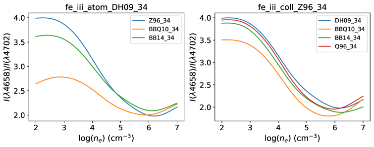
Figure 1: Density behavior of the [Fe iii] $I(\lambda 4658)/I(\lambda 4702)$ emissivity ratio at $T_{e}=7.9\times 10^{3}$ K for different atomic datasets. Left panel: atom_DH09_34 dataset with three coll datasets ( Z96_34, BBQ10_34, and BB14_34). Right panel: coll_Z96_34 dataset with four atom datasets (DH09_34, BBQ10_34, BB14_34, and Q96_34).

For $\log n_{e}\leq 3$, the emissivity ratio $I(\lambda 4658)/I(\lambda 4702)$ is practically density insensitive, being mostly dependent on the ECS of the involved atomic levels. To discern a reliable magnitude in this regime in the light of the discrepancies due to the collisional datasets, we select from the DESIRED database (Méndez-Delgado et al., unpublished) the following low-density sources: 30 Doradus Peimbert (2003); Sh 2-311 García-Rojas et al. (2005); M20 García-Rojas et al. (2006); M17 García-Rojas et al. (2007); HII-1, HII-2, UV-1 López-Sánchez et al. (2007); K932, NGC 5461, NGC 604, NGC 2363, NGC 4861, NGC 1741-C, NGC 5447, VS44, H1013 Esteban et al. (2009); NGC 3125, POX 4, TOL 1924-416, TOL 1457-262, NGC 6822 (HV), NGC 5408 Esteban et al. (2014); Sh 2-100, Sh 2-288 Esteban et al. (2017); NGC 5471, NGC 5455  Esteban et al. (2020), Sh 2-152 Esteban and García-Rojas (2018); and N44C, N11B, N66A, NGC 1714, IC 2111, N81 Domínguez-Guzmán et al. (2022). We then plot the observed line-intensity ratios in Figure 2 as a function of the [S ii] density. In spite of the scatter, there is a definite trend for $I(\lambda 4658)/I(\lambda 4702)>3.5$, which would reinforce the validity of the coll_BB14_34 and coll_Z96_34 datasets.

Regarding a useful [Fe iii] temperature diagnostic, we choose $I(\lambda 4658)/I(\lambda 3240)$ due to its small variations in density and atomic data. In Figure 3, we plot this emissivity ratio as a function of temperature for the same atom–coll grid used in the density diagnostic. The curves show only a weak dependency on the choice of the collisional and radiative datasets.

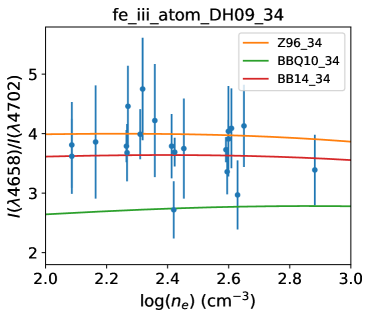
Figure 2: Observed [Fe iii] $I(\lambda 4658)/I(\lambda 4702)$ line-intensity ratio from several low-density sources as a function of the [S ii] density. The theoretical emissivity ratios determined by PyNeb with dataset atom_DH09_34 and three coll datasets (BBQ10_34, BB14_34, and Z96_34) are also depicted.

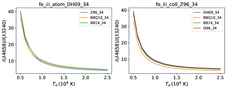
Figure 3: Temperature behavior of the [Fe iii] $I(\lambda 4658)/I(\lambda 3240)$ emissivity ratio at $n_{e}=2.1\times 10^{4}$ cm^-3 for different atomic datasets. Left panel: dataset atom_DH09_34 with three coll datasets (Z96_34, BBQ10_34, and BB14_34). Right panel: dataset coll_Z96_34 with four atom datasets (DH09_34, BBQ10_34, BB14_34, and Q96_34).

A relevant question is whether the density and temperature estimates obtained from the $I(\lambda 4658)/I(\lambda 4702)$ and $I(\lambda 4658)/I(\lambda 3240)$ line ratios, respectively, compare with those obtained from the spectral fits described in Section 3.3.2. For HH 202S, as an example, the observed $I(\lambda 4658)/I(\lambda 4702)=2.81$ and $I(\lambda 4658)/I(\lambda 3240)=13.6$. In the density diagnostic, we set the temperature at $T_{e}=7.9\times 10^{3}$ K and obtain $n_{e}=2.34\times 10^{4}$ cm^-3 for the pair atom_DH09_34–coll_Z96_34 and $n_{e}=1.86\times 10^{4}$ cm^-3 for atom_DH09_34–coll_BB14_34, values that are fairly close to those obtained from the fits, respectively $n_{e}=1.97\times 10^{4}$ cm^-3 and $n_{e}=1.78\times 10^{4}$ cm^-3. However, if we designate the pair atom_DH09_34–coll_BBQ10_34, the theoretical $I(\lambda 4658)/I(\lambda 4702)<2.78$ impairs a density reading for HH 202S. Furthermore, if we set the density at $n_{e}=2.1\times 10^{4}$ cm^-3, we obtain from the temperature diagnostic $7.89\times 10^{3}$ K, $7.95\times 10^{3}$ K, and $8.33\times 10^{3}$ K for the atom–coll pairs DH09_34–Z96_34, DH09_34–BBQ10_34, and DH09_34–BB14_34, respectively, which compare well with $7.71\times 10^{3}$ K, $7.94\times 10^{3}$ K, and $8.18\times 10^{3}$ K from the spectral fits.

3.4 Radiative Lifetimes of $\mathrm{3d^{6}}$ and $\mathrm{3d^{5}4s}$ Levels

As previously mentioned, the [Fe iii] nebular spectrum displays transitions between levels of the $\mathrm{3d^{6}}$ and $\mathrm{3d^{5}4s}$ configurations. The PyNeb Fe iii atomic models are based on the lower 34 levels with $E<60,000$ cm^-1; that is, the cut is imposed just before the onset of the $\mathrm{3d^{5}4s}$ level array. As a result, in the present lifetime analysis, we obviate the $\mathrm{3d^{6}\ b^{1}D_{2}}$ level at 77,044.67 cm^-1 and the unobserved $\mathrm{3d^{6}\ {}^{1}S_{0}}$ estimated theoretically at $E>99,000$ cm^-1. From $\mathrm{3d^{5}4s}$, only the lowly lying $\mathrm{{}^{7}S_{3}}$ and $\mathrm{{}^{5}S_{2}}$ levels are taken into account.

Radiative lifetimes derived from the $A$-values in the atom datasets BB14_34, BBQ10_34, DH09_34, and Q96_34 are compared in Figure 4. For each level, we determine the lifetime differences of these four datasets with respect to the average value. Such differences are, in general, within 0.1 dex except for five levels in atom_BB14_34, nine in atom_BBQ10_34, and two in each atom_DH09_34 and atom_Q96_34. Notably large discrepancies (as large as $\sim 0.8$ dex) are found for the $\mathrm{3d^{6}\,{}^{3}H}_{J}$ levels, which would affect the physical conditions and Fe²⁺ abundance derived from the $\lambda\lambda$4881, 4987, 4924, 5032, 4986 line intensities. Furthermore, the $\mathrm{3d^{6}\ b\,^{3}P}_{J}$ levels in atom_BB14_34 and $\mathrm{3d^{6}\ a\,^{3}P_{2}}$ and $\mathrm{a\,^{1}G_{4}}$ in atom_BBQ10_34 have lifetimes almost 0.2 dex lower. Significant differences also stand out for the $\mathrm{3d^{5}4s\,^{7}S_{3}}$ and $\mathrm{{}^{5}S_{2}}$ levels between these two datasets. A reassuring outcome is the agreement between the atom_DH09_34 and atom_Q96_34 lifetimes: within 20% except for the problematic $\mathrm{{}^{3}H}_{J}$ levels. Most of the conclusions from this comparison are in line with Bautista et al. (2010).

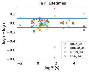
Figure 4: Comparison of Fe iii radiative lifetimes computed from the $A$-values in the atom datasets BB14_34, BBQ10_34, DH09_34, and Q96_34 atom files. For each level, lifetime differences for these datasets with respect to the average value are plotted as a function of the average value.

3.5 Radiative Lifetimes of $\mathrm{3d^{5}4p}$ Levels

Apart from even-parity levels, dataset atom_BB14_144 contains 44 odd-parity levels belonging to the $\mathrm{3d^{5}4p}$ configuration. Their radiative lifetimes can be compared with those derived from the $A$-values computed with extensive CI (single and double excitations up to $n\leq 5$, $\ell\leq 3$, and 6p as well as selective promotions from the 3s and 3p subshells) with the mcbp code civ3  Deb and Hibbert (2009b). As shown in Figure 5, the atom_BB14_144 lifetimes are on average 0.15 dex shorter. The larger differences are found for levels belonging to the $\mathrm{3d^{5}(^{4}P)4p\ ^{3}P^{o}}$, $\mathrm{3d^{5}(^{4}P)4p\ ^{5}P^{o}}$, and $\mathrm{3d^{5}(^{4}D)4p\ ^{5}F^{o}}$ spectroscopic terms.

3.6 Effective Collision Strengths

As shown in Table 5, we have three revised coll datasets containing ECS for the 34-level atomic model of [Fe iii]: Z96_34, BBQ10_34, and BB14_34. We compare these data at $T=10^{4}$ K in Figure 6 using the latter as the reference. In general, there is a reasonable agreement for most transitions, but for several others, huge differences are encountered. Transitions involving the $\mathrm{3d^{5}(^{6}S)4s\ ^{7}S_{3}}$ level are problematic. For instance, in Figure 6 (right panel), we have excluded from coll_Z96_34 transitions of the type $\mathrm{3d^{5}(^{6}S)4s\ ^{7}S_{3}}-\mathrm{3d^{6}}\ ^{1}L_{J}$ as they appear with $\Upsilon=0.0$; furthermore, coll_Z96_34 transitions with $\Delta S=3/2$ have abnormally small ECS ($\log\Upsilon<-4$). These shortcomings may be due to the non-relativistic method used in Zhang (1996). On the other hand, as discussed in Badnell and Ballance (2014), the main differences between the ECS in coll_BBQ10_34 and coll_BB14_34 are due to a mixup by the former in the assignments of the $\mathrm{3d^{5}(^{6}S)4s\ ^{7}S_{3}}$ and $\mathrm{3d^{6}\ {}^{3}G_{3}}$ adjacent levels. Large discrepancies are also found in transitions of the type $\mathrm{3d^{6}\ a\,^{3}P}_{J}-\mathrm{3d^{6}\ {}^{3}H}_{J^{\prime}}$ and $\mathrm{3d^{6}\ b\,^{1}G_{4}}-\mathrm{3d^{6}\ {}^{5}D}_{J}$.

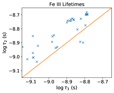
Figure 5: Comparison of radiative lifetimes for 44 levels of the $\mathrm{3d^{5}4p}$ configuration in Fe iii derived from the $A$-values from atom_BB14_144 ($\tau_{1}$) and Ref. Deb and Hibbert (2009b) ($\tau_{2}$).

Figure 6: Comparison of [Fe iii] ECS at $T=10^{4}$ K in the coll_BBQ10_34 and coll_Z96_34 datasets with respect to those in coll_BB14_34.

3.7 Fe iii Discussion

Our initial step in the present atomic data assessment was the comparison of observed line-intensity ratios with the corresponding theoretical $A$-value ratios for transitions arising from a common upper level (see Section 3.3.1). This procedure readily yields a first exposure of observational line misidentifications, blending, and contamination (e.g., telluric or instrumental) and of inherent computational difficulties such as strong valence–core correlation, double-excitation couplings, and strong CI mixing. Therefore, the agreement between theoretical ratios, on the one hand, and between observed and theoretical ratios, on the other hand, are both revealing.

Although the spectra of HH 202S and HH 204 are of comparable quality, the reported observational errors of the former are on average larger (36%) than the latter (12%). Comparisons among theoretical $A$-value ratios and with the observed counterparts lead to an overall accuracy level for the theoretical ratios of around 20–30%, except for odd theoretical outliers pinpointed in Section 3.3.1 believed to be caused by the aforementioned computational difficulties.

The spectrum fits performed in Section 3.3.2 bring to the fore a frequent drawback in modeling codes: the error-prone mapping of radiative or collisional datasets onto an atomic model with different level numbering as illustrated with dataset coll_BB14 that led to file deprecation. The four revised atom datasets (BBQ10_34, BB14_34, DH09_34, Q96_34) and three coll datasets (BBQ10_34, BB14_34, Z96_34) appear to give comparable temperatures and densities within error bands of 6% and 20%, respectively, which also match satisfactorily estimates obtained from [Fe iii] line-ratio diagnostics such as $I(\lambda 4658)/I(\lambda 4702)$ and $I(\lambda 4658)/I(\lambda 3240)$ (see Section 3.3.3) and from alternative ionic diagnostics reported in Mesa-Delgado et al. (2009); Méndez-Delgado et al. (2021b). However, the density-sensitive ratio $I(\lambda 4658)/I(\lambda 4702)$ computed with coll_BBQ10_34 does not match the ratios observed in low-density ($\log n_{e}\lesssim 3$) nebular sources (see Figure 2).

As shown in Section 3.4, radiative lifetimes for levels of the $\mathrm{3d^{6}}$ and $\mathrm{3d^{5}4s}$ configurations computed with $A$-values from the BBQ10_34, BB14_34, DH09_34, and Q96_34 atom datasets agree to within $\sim 0.1$ dex except for $\mathrm{3d^{6}\ {}^{3}H_{J}}$ and $\mathrm{3d^{5}4s\ ^{7}S_{J},^{5}S_{2}}$. However, the best agreement ($\sim 20\%$) is found between $A$-values from structure calculations, namely atom_DH09_34 and atom_Q96_34, rather than those associated with scattering targets. This may be due to the convergence and accuracy of the CI expansions implemented in each calculation type. In structure calculations of radiative lifetimes for transitions involving levels of the $\mathrm{3d^{6}}$ and $\mathrm{3d^{5}4s}$ configurations in Fe iii, for instance, there is no need to include odd-parity configurations, while in a Fe iii scattering target, a reduced set of configurations of both parity types must be considered. A similar argument may be applied to the lifetimes of $\mathrm{3d^{5}4p}$ levels (see Section 3.5), where the atom_BB14_144 lifetimes are on average shorter than those from a lengthy mcbp structure calculation Deb and Hibbert (2009b).

The main finding of the ECS comparison in Section 3.6 is the large discrepancies displayed by coll_Z96_34 ECS with respect to coll_BB14_34 for some transitions with $\log\Upsilon<-1$ (see Figure 6), which may be due to the non-relativistic $R$-matrix method used by Zhang (1996) in the computation of the former dataset. The larger ECS differences between coll_BBQ10_34 and coll_BB14_34 are mainly due to level misassignments.

Analyzing results from these data comparisons and spectral fits, we select as the [Fe iii] default datasets in PyNeb 1.1.17 the atom_BB14_144 and coll_BB14_144 files, while files coll_BBQ10 and coll_BB14 are deprecated. Deprecated files are still available with the command
pn.atomicData.includeDeprecatedPath(). Files atom_BBQ10 and coll_Z96 remain active, and files coll_BBQ10_34, atom_BB14_144, atom_DH09_34, and atom_Q96_34 are incorporated.

4 Fe ii

Similarly to the Fe iii atomic data assessment, we implement observational benchmarks to evaluate the atomic datasets for Fe ii  available in PyNeb 1.1.16, transcribing them directly from the source and implementing new models. NIST energy levels in this version of PyNeb are the same as those listed in the database of July 2022 Kramida et al. (2021).

4.1 Fe ii Atomic Datasets in PyNeb

The following datasets are available for Fe ii in PyNeb 1.1.16:

atom_VVKFHF99, coll_VVKFHF99

—These datasets list radiative and collisional rates for transitions among 80 levels with energies $E<44,760$ cm^-1 compiled from different sources Verner et al. (1999). $A$-values for the dipole allowed and forbidden transitions are from Nahar (1995) and Quinet et al. (1996), respectively. ECS are mainly from Zhang and Pradhan (1995); however, the source data are not available and $A$-values and ECS for transitions with spin change $\Delta S=2$ have been obviated.

atom_B15, coll_B15

—$A$-values and ECS for transitions among 52 levels belonging to the $\mathrm{3d^{7}}$, $\mathrm{3d^{6}4s}$, and $\mathrm{3d^{5}4s^{2}}$ configurations ($E<31,500$ cm^-1) Bautista et al. (2015). $A$-values were computed with the mcbp atomic structure code autostructure using different expansions and orbital optimization strategies and a dipole correction to the Thomas–Fermi–Dirac–Amaldi potential. Fine-tuning was carried out by means of term-energy corrections adjusted by fitting to the experimental term energies. ECS were computed with the Dirac–Coulomb $R$-matrix package darc Ait-Tahar et al. (1996) using a target generated with the fully relativistic atomic structure code grasp0 Parpia et al. (1996) using a six-configuration expansion comprising 329 levels.

atom_SRKFB19, coll_SRKFB19

—$A$-values and ECS for 250 levels from the $\mathrm{3d^{7}}$, $\mathrm{3d^{6}4s}$, $\mathrm{3d^{5}4s^{2}}$, $\mathrm{3d^{6}4p}$, and $\mathrm{3d^{5}4s4p}$ configurations Smyth et al. (2019). $A$-values were computed with grasp0 in a 20-configuration expansion and ECS with darc using a 716-level target representation.

4.2 Fe ii Revised and New Atomic Datasets

For comparison purposes, models were normalized to 52 levels ($E<31,500$ cm^-1), i.e., the number of levels considered in atom_B15 that includes the last even quartet term before the appearance of the $\mathrm{3d^{6}4p}$ level array. Two datasets have been extended to comprise 173 levels ($E<66,100$ cm^-1), a cut before the onset of unmeasured levels in the NIST level list, and 225 levels ($E<73,800$ cm^-1) to discuss some assignment inconsistencies. Although ECS from Zhang and Pradhan (1995) are included in VVKFHF99, we have not considered their dataset individually as it excludes the doublet terms in their atomic model.

atom_QDZa96, atom_QDZh96

—E2 and M1 $A$-values calculated for transitions among the 63 levels of the configurations $\mathrm{3d^{6}4s}$, $\mathrm{3d^{7}}$, and $\mathrm{3d^{5}4s^{2}}$ Quinet et al. (1996). Extensive CI expansion was used with the Breit–Pauli superstructure Eissner et al. (1974) (QDZa96) and Pauli hfr Cowan (1981) (QDZh96) atomic structure codes. These datasets are not complete enough to be used in PyNeb spectral modeling as they obviate transitions such as $\mathrm{a\,^{4}F-a\,^{6}D}$ and $\mathrm{a\,^{2}P-a\,^{6}D}$; therefore, they will only be used in radiative data comparisons.

atom_VVKFHF99_52, coll_VVKFHF99_52

—The VVKFHF99 datasets containing $A$-values and ECS described in Section 4.1 are reduced to 52 levels from even-parity configurations.

atom_DH11_52

—E2 and M1 $A$-values for transitions between levels of the $\mathrm{3d^{6}4s}$, $\mathrm{3d^{7}}$, and $\mathrm{3d^{5}4s^{2}}$ configurations were computed in a large-scale CI framework with the mcbp structure code civ3 Deb and Hibbert (2011). Wave functions were fine-tuned to fit the experimental energies.

atom_B15_52, coll_B15_52

—Data ($A$-values and ECS) from the B15 calculation described in Section 4.1 were downloaded directly from the CDS, and the datasets were reconstructed.

atom_TZ18_52, coll_TZ18_52

—$A$-values and ECS were computed with the close-coupling $B$-spline Breit–Pauli $R$-matrix method for 340 levels of the $\mathrm{3d^{6}4s}$, $\mathrm{3d^{7}}$, $\mathrm{3d^{5}4s^{2}}$, $\mathrm{3d^{6}4p}$, and $\mathrm{3d^{5}4s4p}$ configurations Tayal and Zatsarinny (2018). The CI target representation was constructed with a Hartree–Fock method. Semi-empirical fine-tuning in the structure and scattering calculations was introduced by fitting tothe experimental energies. The final Hamiltonian of the scattering calculation contains the spin–orbit term.

atom_SRKFB19_52, coll_SRKFB19_52

—Radiative and collisional data from the SRKFB19 calculation were described in Section 4.1. New files were constructed with data extracted from the adf04_DARC716_2.10.18 file (Cathy Ramsbottom, private communication) and reduced to 52 levels.

atom_SRKFB19_173, coll_SRKFB19_173, atom_TZ18_173, coll_TZ18_173

—The SRKFB19 and TZ18 datasets have been extended to 173 levels ($E<66,100$ cm^-1) to test model convergence.

atom_SRKFB19_225, atom_TZ18_225

—The theoretical SRKFB19 and TZ18 datasets have been extended to 225 levels ($E<73,800$ cm^-1) to bring out term assignment inconsistencies involving levels with total orbital angular momentum quantum number $L=5$ (see Table 6). With respect to NIST and other theoretical datasets, the term assignments of levels at $21,430.36$ and $21,581.62$ cm^-1 ($\mathrm{a\,^{4}H}$) and $26,170.18$ and $26,352.77$ cm^-1 ($\mathrm{b\,^{2}H}$) have been interchanged in atom_SRKFB19_225. Since the total angular momentum quantum number $J$ of each level coincides in the different datasets, the incongruent term labeling would be inconsequential if the $A$-values for the transitions involving these levels were comparable. As shown in Table 7, this is not the case, as discrepancies as large as an order of magnitude were encountered. A similar mixup was found with the odd-parity $\mathrm{z\,^{4}H^{o}}$ and $\mathrm{y\,^{2}H^{o}}$ levels, which in this case are even energetically misplaced (see Table 6). Assignment discrepancies of this sort could be due to strong CI admixture in terms with high orbital angular momentum ($L>4$ say) in lowly ionized systems that the grasp0 multi-configuration Dirac–Hartree–Fock structure code has problems resolving.

Table 6: Comparison of NIST energies (cm^-1) for levels in Fe ii displaying a total orbital angular momentum quantum number $L=5$ with those listed in different atom datasets (see Section 4.2). Questionable level assignments are found in atom_SRKFB19_225.

Level	NIST	SRKFB19_225	TZ18_225	DH11_52	B15_52	QDZh96
$\mathrm{3d^{7}\ a\,^{2}H_{11/2}}$	20,340.25	20,340.25	20,327.91	20,340.30	20,340.30	20,340
$\mathrm{3d^{7}\ a\,^{2}H_{9/2}}$	20,805.76	20,805.76	20,824.99	20,805.77	20,805.77	20,806
$\mathrm{3d^{6}(^{3}H)4s\ a\,^{4}H_{13/2}}$	21,251.58	21,251.58	21,283.52	21,251.61	21,251.61	21,252
$\mathrm{3d^{6}(^{3}H)4s\ a\,^{4}H_{11/2}}$	21,430.36	26,170.17	21,433.70	21,430.36	21,430.36	21,430
$\mathrm{3d^{6}(^{3}H)4s\ a\,^{4}H_{9/2}}$	21,581.62	26,352.77	21,560.17	21,581.64	21,581.64	21,582
$\mathrm{3d^{6}(^{3}H)4s\ a\,^{4}H_{7/2}}$	21,711.90	21,711.90	21,671.63	21,711.92	21,711.92	21,712
$\mathrm{3d^{6}(^{3}H)4s\ b\,^{2}H_{11/2}}$	26,170.18	21,430.36	26,186.48	26,170.18	26,170.18	26,170
$\mathrm{3d^{6}(^{3}H)4s\ b\,^{2}H_{9/2}}$	26,352.77	21,581.61	26,331.50	26,352.77	26,352.77	26,353
$\mathrm{3d^{6}(^{3}H)4p\ z\,^{4}H^{o}_{13/2}}$	60,837.56	60,837.55	60,832.43
$\mathrm{3d^{6}(^{3}H)4p\ z\,^{4}H^{o}_{11/2}}$	60,887.61		60,880.58
$\mathrm{3d^{6}(^{3}H)4p\ z\,^{4}H^{o}_{9/2}}$	60,989.44		61,012.21
$\mathrm{3d^{6}(^{3}H)4p\ z\,^{4}H^{o}_{7/2}}$	61,156.83	61,156.82	61,178.84
$\mathrm{3d^{6}(^{3}H)4p\ z\,^{2}H^{o}_{11/2}}$	65,363.61	65,363.60	65,333.65
$\mathrm{3d^{6}(^{3}H)4p\ z\,^{2}H^{o}_{9/2}}$	65,556.27	65,556.26	65,551.82
$\mathrm{3d^{6}(^{3}G)4p\ y\,^{4}H^{o}_{13/2}}$	66,411.71	66,411.70	66,306.76
$\mathrm{3d^{6}(^{3}G)4p\ y\,^{4}H^{o}_{11/2}}$	66,463.54	66,463.54	66,602.84
$\mathrm{3d^{6}(^{3}G)4p\ y\,^{4}H^{o}_{9/2}}$	66,589.04	66,589.03	66,733.10
$\mathrm{3d^{6}(^{3}G)4p\ y\,^{4}H^{o}_{7/2}}$	66,672.34	66,672.32	66,705.11
$\mathrm{3d^{6}(^{3}G)4p\ y\,^{2}H^{o}_{11/2}}$	67,516.33	67,516.32	67,942.69
$\mathrm{3d^{6}(^{3}G)4p\ y\,^{2}H^{o}_{11/2}}$		67,709.96
$\mathrm{3d^{6}(^{3}G)4p\ y\,^{2}H^{o}_{9/2}}$	68,000.79	68,000.77	67,609.99
$\mathrm{3d^{6}(^{3}G)4p\ y\,^{2}H^{o}_{9/2}}$		68,201.16
$\mathrm{3d^{6}(^{1}G2)4p\ x\,^{2}H^{o}_{9/2}}$	72,130.38	72,130.36	72,407.94
$\mathrm{3d^{6}(^{1}G2)4p\ x\,^{2}H^{o}_{11/2}}$	72,261.74	72,261.73	71,962.96
$\mathrm{3d^{6}(^{1}I)4p\ w\,^{2}H^{o}_{11/2}}$	73,603.54	73,603.53	73,435.97
$\mathrm{3d^{6}(^{1}I)4p\ w\,^{2}H^{o}_{9/2}}$	73,751.28	73,751.27	73,868.28

Table 7: $A$-values for transitions arising from the $\mathrm{3d^{6}4s\ a\,^{4}H_{J}}$ and $\mathrm{3d^{6}4s\ b\,^{2}H_{J}}$ levels ($J=9/2$ and $11/2$) upper levels of [Fe ii] listed in different atom datasets, which show the large discrepancies in atom_SRKFB19_225.

$\lambda_{\mathrm{air}}$ (Å)	$A$-Value (s-1)
	SRKFB19_225	TZ18_225	DH11_52	B15_52	QDZa96	QDZh96
4114.48	$1.52\times 10^{-2}$	$1.44\times 10^{-1}$	$1.61\times 10^{-1}$	$1.05\times 10^{-1}$	$7.80\times 10^{-2}$	$1.03\times 10^{-1}$
4178.96	$7.45\times 10^{-4}$	$3.26\times 10^{-2}$	$2.02\times 10^{-2}$	$1.89\times 10^{-2}$	$9.95\times 10^{-3}$	$1.56\times 10^{-2}$
4211.11	$1.81\times 10^{-2}$	$5.40\times 10^{-2}$	$5.93\times 10^{-2}$	$3.15\times 10^{-2}$	$3.37\times 10^{-2}$	$4.44\times 10^{-2}$
4251.45	$6.12\times 10^{-3}$	$2.86\times 10^{-2}$	$1.96\times 10^{-2}$	$1.33\times 10^{-2}$	$1.28\times 10^{-2}$	$1.87\times 10^{-2}$
5111.64	$4.68\times 10^{-1}$	$1.01\times 10^{-1}$	$1.07\times 10^{-1}$	$1.19\times 10^{-1}$	$1.20\times 10^{-1}$	$1.31\times 10^{-1}$
5220.08	$8.90\times 10^{-2}$	$1.09\times 10^{-1}$	$1.11\times 10^{-1}$	$1.32\times 10^{-1}$	$1.34\times 10^{-1}$	$1.44\times 10^{-1}$
5261.63	$1.62\times 10^{+0}$	$3.25\times 10^{-1}$	$3.39\times 10^{-1}$	$3.95\times 10^{-1}$	$4.01\times 10^{-1}$	$4.29\times 10^{-1}$
5333.66	$8.85\times 10^{-1}$	$2.68\times 10^{-1}$	$2.78\times 10^{-1}$	$3.23\times 10^{-1}$	$3.32\times 10^{-1}$	$3.51\times 10^{-1}$

4.3 Observational and Spectroscopic Benchmarks

Due to the wide astrophysical interest in Fe ii, this ion presents interesting possibilities for implementing observational and spectroscopic benchmarks. There is interest not only in the forbidden-line spectrum but also in the allowed transition arrays involving levels from the odd-parity configurations $\mathrm{3d^{6}4p}$ and $\mathrm{3d^{5}4s4p}$, which may be populated by fluorescence pumping from the stellar continuum Rodríguez (1999); Verner et al. (2000); Hartman (2013). Fe ii ultraviolet emission in active galactic nuclei is not fully understood, impeding quasar classification schemes and Fe abundance estimates Sarkar et al. (2021).

4.3.1 $A$-Value Ratio Benchmark

In Tables 8 and 9, we compare the observed line-intensity ratios in the spectra of HH 202S and HH 204 involving transitions from a common upper level with the corresponding $A$-value ratios (see Equation (1)) from atom datasets B15_52, DH11_52, TZ18_52, SRKFB19_52, QDZa96, and QDZh96. In this comparison, we must point out the worrisome discrepancies displayed by some $A$-value ratios from atom_SRKFB19_52 with both the observed and other theoretical values; thus, the integrity of this radiative dataset is questionable.

Table 8: Comparison of [Fe ii] line-intensity ratios for transitions arising from a common upper level in the HH 202S spectrum (Obs) with those estimated from $A$-values in the following atom datasets: B15_52 (T1); DH11_52 (T2); TZ18_52 (T3); SRKFB19_52 (T4); QDZa96 (T5); QDZh96 (T6). The error of the least significant figure of the observed intensity ratio is indicated in brackets.

Line 1			Line 2		Obs	T1	T2	T3	T4	T5	T6
Upper	Lower	$\lambda_{\mathrm{air}}$(Å)	Lower	$\lambda_{\mathrm{air}}$(Å)	Line Intensity Ratio
$\mathrm{b\ ^{2}H_{9/2}}$	$\mathrm{a\ ^{4}F_{7/2}}$	4178.96	$\mathrm{a\ ^{4}F_{5/2}}$	4251.45	1.3(9)	1.44	1.05	1.16	0.12	0.79	0.85
$\mathrm{b\ ^{2}H_{11/2}}$	$\mathrm{a\ ^{4}F_{9/2}}$	4114.48	$\mathrm{a\ ^{4}F_{7/2}}$	4211.11	2.4(8)	3.42	2.78	2.73	0.86	2.37	2.37
$\mathrm{a\ ^{4}G_{7/2}}$	$\mathrm{a\ ^{4}F_{5/2}}$	4319.62	$\mathrm{a\ ^{4}F_{3/2}}$	4372.43	2.4(8)	2.00	1.95	1.97	1.88	1.98	1.96
$\mathrm{a\ ^{4}G_{9/2}}$	$\mathrm{a\ ^{4}F_{9/2}}$	4177.20	$\mathrm{a\ ^{4}F_{7/2}}$	4276.84	0.28(8)	0.24	0.21	0.23	0.29	0.25	0.24
$\mathrm{a\ ^{4}G_{9/2}}$	$\mathrm{a\ ^{4}F_{7/2}}$	4276.84	$\mathrm{a\ ^{4}F_{5/2}}$	4352.78	2.1(6)	2.16	2.15	2.24	2.07	2.21	2.19
$\mathrm{a\ ^{4}G_{11/2}}$	$\mathrm{a\ ^{4}F_{9/2}}$	4243.97	$\mathrm{a\ ^{4}F_{7/2}}$	4346.86	5(1)	4.40	4.54	4.67	4.24	4.60	4.59
$\mathrm{a\ ^{6}S_{5/2}}$	$\mathrm{a\ ^{6}D_{9/2}}$	4287.39	$\mathrm{a\ ^{6}D_{7/2}}$	4359.33	1.3(3)	1.37	1.37	1.38	1.35	1.37	1.38
$\mathrm{a\ ^{6}S_{5/2}}$	$\mathrm{a\ ^{6}D_{7/2}}$	4359.33	$\mathrm{a\ ^{6}D_{5/2}}$	4413.78	1.4(3)	1.44	1.43	1.44	1.42	1.42	1.44
$\mathrm{a\ ^{6}S_{5/2}}$	$\mathrm{a\ ^{6}D_{5/2}}$	4413.78	$\mathrm{a\ ^{6}D_{3/2}}$	4452.10	1.6(4)	1.58	1.57	1.58	1.56	1.57	1.58
$\mathrm{a\ ^{6}S_{5/2}}$	$\mathrm{a\ ^{6}D_{3/2}}$	4452.10	$\mathrm{a\ ^{6}D_{1/2}}$	4474.90	2.2(7)	2.07	2.06	2.06	2.05	2.06	2.06
$\mathrm{b\ ^{4}F_{3/2}}$	$\mathrm{a\ ^{6}D_{3/2}}$	4509.61	$\mathrm{a\ ^{4}F_{5/2}}$	4950.76	0.4(2)	0.31	0.40	0.38	0.11	0.28	0.28
$\mathrm{b\ ^{4}F_{3/2}}$	$\mathrm{a\ ^{4}F_{5/2}}$	4950.76	$\mathrm{a\ ^{4}F_{3/2}}$	5020.24	0.9(4)	0.96	0.97	0.98	0.95	0.97	0.97
$\mathrm{b\ ^{4}F_{5/2}}$	$\mathrm{a\ ^{6}D_{7/2}}$	4432.45	$\mathrm{a\ ^{6}D_{5/2}}$	4488.75	0.6(3)	0.36	0.36	0.36	0.36	0.37	0.36
$\mathrm{b\ ^{4}F_{5/2}}$	$\mathrm{a\ ^{6}D_{5/2}}$	4488.75	$\mathrm{a\ ^{6}D_{3/2}}$	4528.38	3(2)	3.44	3.44	3.43	3.38	3.42	3.45
$\mathrm{b\ ^{4}F_{5/2}}$	$\mathrm{a\ ^{6}D_{3/2}}$	4528.38	$\mathrm{a\ ^{4}F_{7/2}}$	4874.50	0.3(2)	0.23	0.30	0.28	0.09	0.22	0.21
$\mathrm{b\ ^{4}F_{5/2}}$	$\mathrm{a\ ^{4}F_{7/2}}$	4874.50	$\mathrm{a\ ^{4}F_{5/2}}$	4973.40	1.3(5)	1.25	1.24	1.27	1.26	1.26	1.24
$\mathrm{b\ ^{4}F_{5/2}}$	$\mathrm{a\ ^{4}F_{5/2}}$	4973.40	$\mathrm{a\ ^{4}F_{3/2}}$	5043.53	1.5(7)	2.01	2.07	1.99	1.61	1.93	1.97
$\mathrm{b\ ^{4}F_{7/2}}$	$\mathrm{a\ ^{6}D_{7/2}}$	4457.95	$\mathrm{a\ ^{6}D_{5/2}}$	4514.90	4(2)	4.30	4.35	4.32	4.22	4.30	4.34
$\mathrm{b\ ^{4}F_{7/2}}$	$\mathrm{a\ ^{6}D_{5/2}}$	4514.90	$\mathrm{a\ ^{4}F_{9/2}}$	4774.73	0.6(3)	0.46	0.60	0.56	0.19	0.44	0.42
$\mathrm{b\ ^{4}F_{7/2}}$	$\mathrm{a\ ^{4}F_{9/2}}$	4774.73	$\mathrm{a\ ^{4}F_{7/2}}$	4905.35	0.6(2)	0.58	0.58	0.60	0.72	0.59	0.59
$\mathrm{b\ ^{4}F_{9/2}}$	$\mathrm{a\ ^{6}D_{9/2}}$	4416.27	$\mathrm{a\ ^{6}D_{7/2}}$	4492.64	7(2)	7.61	7.54	7.70	7.41	7.60	7.74
$\mathrm{b\ ^{4}F_{9/2}}$	$\mathrm{a\ ^{6}D_{7/2}}$	4492.64	$\mathrm{a\ ^{4}F_{9/2}}$	4814.54	0.15(5)	0.14	0.19	0.17	0.07	0.13	0.12
$\mathrm{b\ ^{4}F_{9/2}}$	$\mathrm{a\ ^{4}F_{9/2}}$	4814.54	$\mathrm{a\ ^{4}F_{7/2}}$	4947.39	7(2)	7.57	6.35	7.00	0.88	7.09	7.17
$\mathrm{b\ ^{4}F_{9/2}}$	$\mathrm{a\ ^{4}F_{7/2}}$	4947.39	$\mathrm{a\ ^{4}D_{7/2}}$	6809.24	4(2)	3.49	3.22	3.07	70.2	3.98	4.16
$\mathrm{b\ ^{4}P_{3/2}}$	$\mathrm{a\ ^{6}D_{5/2}}$	4728.07	$\mathrm{a\ ^{4}F_{7/2}}$	5158.01	0.9(3)	1.23	1.83	2.00	0.57	1.29	1.19
$\mathrm{b\ ^{4}P_{3/2}}$	$\mathrm{a\ ^{4}F_{7/2}}$	5158.01	$\mathrm{a\ ^{4}F_{5/2}}$	5268.89	3(1)	1.57	1.56	1.57	1.48	1.57	1.56
$\mathrm{a\ ^{4}H_{7/2}}$	$\mathrm{a\ ^{4}F_{5/2}}$	5296.84	$\mathrm{a\ ^{4}F_{3/2}}$	5376.47	0.3(1)	0.32	0.34	0.34	0.13	0.34	0.34
$\mathrm{a\ ^{4}H_{9/2}}$	$\mathrm{a\ ^{4}F_{7/2}}$	5220.08	$\mathrm{a\ ^{4}F_{5/2}}$	5333.66	0.4(1)	0.42	0.41	0.42	0.10	0.41	0.42
$\mathrm{a\ ^{4}H_{11/2}}$	$\mathrm{a\ ^{4}F_{9/2}}$	5111.64	$\mathrm{a\ ^{4}F_{7/2}}$	5261.63	0.32(6)	0.31	0.32	0.32	0.30	0.31	0.31
$\mathrm{a\ ^{2}D2_{3/2}}$	$\mathrm{a\ ^{6}D_{3/2}}$	4889.71	$\mathrm{a\ ^{4}F_{5/2}}$	5412.68	3(1)	0.00	0.00	0.00	0.00	0.00	0.00
$\mathrm{a\ ^{2}D2_{3/2}}$	$\mathrm{a\ ^{4}F_{5/2}}$	5412.68	$\mathrm{a\ ^{4}F_{3/2}}$	5495.84	2(1)	1.89	1.91	1.90	1.89	1.89	1.90
$\mathrm{b\ ^{4}P_{5/2}}$	$\mathrm{a\ ^{4}F_{9/2}}$	5273.36	$\mathrm{a\ ^{4}F_{7/2}}$	5433.15	3(1)	3.32	2.88	3.19	3.27	3.28	3.26
$\mathrm{a\ ^{2}D2_{5/2}}$	$\mathrm{a\ ^{4}F_{7/2}}$	5527.35	$\mathrm{a\ ^{4}F_{5/2}}$	5654.87	10(4)	9.26	9.09	9.19	9.12	9.06	8.98
$\mathrm{a\ ^{2}G_{7/2}}$	$\mathrm{a\ ^{4}F_{7/2}}$	7172.00	$\mathrm{a\ ^{4}F_{5/2}}$	7388.17	1.4(3)	1.35	1.35	1.36	1.32	1.35	1.35
$\mathrm{a\ ^{2}G_{9/2}}$	$\mathrm{a\ ^{4}F_{9/2}}$	7155.17	$\mathrm{a\ ^{4}F_{7/2}}$	7452.56	3.1(5)	3.17	3.22	3.23	3.10	3.19	3.24
$\mathrm{a\ ^{4}P_{1/2}}$	$\mathrm{a\ ^{4}F_{5/2}}$	9033.49	$\mathrm{a\ ^{4}F_{3/2}}$	9267.55	0.8(2)	0.77	0.78	0.78	0.50	0.78	0.78
$\mathrm{a\ ^{4}P_{3/2}}$	$\mathrm{a\ ^{6}D_{5/2}}$	7686.93	$\mathrm{a\ ^{4}F_{7/2}}$	8891.93	0.27(7)	0.26	0.83	0.44	0.40	0.36	0.44
$\mathrm{a\ ^{4}P_{3/2}}$	$\mathrm{a\ ^{4}F_{7/2}}$	8891.93	$\mathrm{a\ ^{4}F_{5/2}}$	9226.63	1.7(3)	1.76	1.79	1.78	0.88	1.78	1.80
$\mathrm{a\ ^{4}P_{5/2}}$	$\mathrm{a\ ^{6}D_{7/2}}$	7637.52	$\mathrm{a\ ^{4}F_{7/2}}$	9051.95	0.5(1)	0.59	1.96	1.08	0.18	0.89	1.15
$\mathrm{a\ ^{4}P_{5/2}}$	$\mathrm{a\ ^{4}F_{7/2}}$	9051.95	$\mathrm{a\ ^{4}F_{5/2}}$	9399.04	7(2)	5.13	5.32	5.21	2.64	5.46	5.67

Table 9: Comparison of [Fe ii] line-intensity ratios for transitions arising from a common upper level in the HH 204 spectrum (Obs) with those estimated from $A$-values in the following atom datasets: B15_52 (T1); DH11_52 (T2); TZ18_52 (T3); SRKFB19_52 (T4); QDZa96 (T5); QDZh96 (T6). The error of the least significant figure of the observed intensity ratio is indicated in brackets.

Line 1			Line 2		Obs	T1	T2	T3	T4	T5	T6
Upper	Lower	$\lambda_{\mathrm{air}}$(Å)	Lower	$\lambda_{\mathrm{air}}$(Å)	Line Intensity Ratio
$\mathrm{a\ ^{2}F_{7/2}}$	$\mathrm{a\ ^{4}D_{7/2}}$	5163.96	$\mathrm{a\ ^{2}G_{9/2}}$	8715.80	9(2)	7.50	10.5	11.1	2.81	6.73	7.48
$\mathrm{b\ ^{2}H_{9/2}}$	$\mathrm{a\ ^{4}F_{7/2}}$	4178.96	$\mathrm{a\ ^{4}F_{5/2}}$	4251.45	1.2(2)	1.44	1.05	1.16	0.12	0.79	0.85
$\mathrm{b\ ^{2}H_{11/2}}$	$\mathrm{a\ ^{4}F_{9/2}}$	4114.48	$\mathrm{a\ ^{4}F_{7/2}}$	4211.11	2.6(2)	3.42	2.78	2.73	0.86	2.37	2.37
$\mathrm{a\ ^{4}G_{5/2}}$	$\mathrm{a\ ^{6}D_{3/2}}$	3968.27	$\mathrm{a\ ^{4}F_{5/2}}$	4305.90	7(1)	0.00	0.00	0.00	0.00	0.00	0.00
$\mathrm{a\ ^{4}G_{5/2}}$	$\mathrm{a\ ^{4}F_{5/2}}$	4305.90	$\mathrm{a\ ^{4}F_{3/2}}$	4358.37	0.56(8)	0.44	0.42	0.44	0.48	0.46	0.45
$\mathrm{a\ ^{4}G_{7/2}}$	$\mathrm{a\ ^{4}F_{5/2}}$	4319.62	$\mathrm{a\ ^{4}F_{3/2}}$	4372.43	2.0(2)	2.00	1.95	1.97	1.88	1.98	1.96
$\mathrm{a\ ^{4}G_{9/2}}$	$\mathrm{a\ ^{4}F_{9/2}}$	4177.20	$\mathrm{a\ ^{4}F_{7/2}}$	4276.84	0.25(2)	0.24	0.21	0.23	0.29	0.25	0.24
$\mathrm{a\ ^{4}G_{9/2}}$	$\mathrm{a\ ^{4}F_{7/2}}$	4276.84	$\mathrm{a\ ^{4}F_{5/2}}$	4352.78	2.1(1)	2.16	2.15	2.24	2.07	2.21	2.19
$\mathrm{a\ ^{4}G_{11/2}}$	$\mathrm{a\ ^{4}F_{9/2}}$	4243.97	$\mathrm{a\ ^{4}F_{7/2}}$	4346.86	4.9(2)	4.40	4.54	4.67	4.24	4.60	4.59
$\mathrm{a\ ^{6}S_{5/2}}$	$\mathrm{a\ ^{6}D_{9/2}}$	4287.39	$\mathrm{a\ ^{6}D_{7/2}}$	4359.33	1.39(6)	1.37	1.37	1.38	1.35	1.37	1.38
$\mathrm{a\ ^{6}S_{5/2}}$	$\mathrm{a\ ^{6}D_{7/2}}$	4359.33	$\mathrm{a\ ^{6}D_{5/2}}$	4413.78	1.42(6)	1.44	1.43	1.44	1.42	1.42	1.44
$\mathrm{a\ ^{6}S_{5/2}}$	$\mathrm{a\ ^{6}D_{5/2}}$	4413.78	$\mathrm{a\ ^{6}D_{3/2}}$	4452.10	1.55(6)	1.58	1.57	1.58	1.57	1.57	1.58
$\mathrm{a\ ^{6}S_{5/2}}$	$\mathrm{a\ ^{6}D_{3/2}}$	4452.10	$\mathrm{a\ ^{6}D_{1/2}}$	4474.90	2.0(1)	2.07	2.06	2.06	2.05	2.06	2.06
$\mathrm{b\ ^{4}F_{3/2}}$	$\mathrm{a\ ^{6}D_{3/2}}$	4509.61	$\mathrm{a\ ^{4}F_{5/2}}$	4950.76	0.42(9)	0.31	0.40	0.38	0.11	0.28	0.28
$\mathrm{b\ ^{4}F_{3/2}}$	$\mathrm{a\ ^{4}F_{5/2}}$	4950.76	$\mathrm{a\ ^{4}F_{3/2}}$	5020.24	1.4(3)	0.96	0.97	0.98	0.95	0.97	0.97
$\mathrm{b\ ^{4}F_{5/2}}$	$\mathrm{a\ ^{6}D_{7/2}}$	4432.45	$\mathrm{a\ ^{6}D_{5/2}}$	4488.75	0.49(7)	0.36	0.36	0.36	0.36	0.37	0.36
$\mathrm{b\ ^{4}F_{5/2}}$	$\mathrm{a\ ^{6}D_{5/2}}$	4488.75	$\mathrm{a\ ^{6}D_{3/2}}$	4528.38	3.6(7)	3.44	3.44	3.43	3.38	3.42	3.45
$\mathrm{b\ ^{4}F_{5/2}}$	$\mathrm{a\ ^{6}D_{3/2}}$	4528.38	$\mathrm{a\ ^{4}F_{7/2}}$	4874.50	0.25(5)	0.23	0.30	0.28	0.09	0.22	0.21
$\mathrm{b\ ^{4}F_{5/2}}$	$\mathrm{a\ ^{4}F_{7/2}}$	4874.50	$\mathrm{a\ ^{4}F_{5/2}}$	4973.40	1.4(1)	1.25	1.24	1.27	1.26	1.26	1.24
$\mathrm{b\ ^{4}F_{5/2}}$	$\mathrm{a\ ^{4}F_{5/2}}$	4973.40	$\mathrm{a\ ^{4}F_{3/2}}$	5043.53	1.9(3)	2.01	2.07	1.99	1.61	1.93	1.97
$\mathrm{b\ ^{4}F_{7/2}}$	$\mathrm{a\ ^{6}D_{9/2}}$	4382.74	$\mathrm{a\ ^{6}D_{7/2}}$	4457.95	0.19(2)	0.20	0.21	0.20	0.20	0.21	0.20
$\mathrm{b\ ^{4}F_{7/2}}$	$\mathrm{a\ ^{6}D_{7/2}}$	4457.95	$\mathrm{a\ ^{6}D_{5/2}}$	4514.90	4.3(4)	4.30	4.35	4.32	4.22	4.30	4.34
$\mathrm{b\ ^{4}F_{7/2}}$	$\mathrm{a\ ^{6}D_{5/2}}$	4514.90	$\mathrm{a\ ^{4}F_{9/2}}$	4774.73	0.56(6)	0.46	0.60	0.56	0.19	0.44	0.42
$\mathrm{b\ ^{4}F_{7/2}}$	$\mathrm{a\ ^{4}F_{9/2}}$	4774.73	$\mathrm{a\ ^{4}F_{7/2}}$	4905.35	0.57(4)	0.58	0.58	0.60	0.72	0.59	0.59
$\mathrm{b\ ^{4}F_{9/2}}$	$\mathrm{a\ ^{6}D_{9/2}}$	4416.27	$\mathrm{a\ ^{6}D_{7/2}}$	4492.64	7.7(5)	7.61	7.54	7.70	7.41	7.60	7.74
$\mathrm{b\ ^{4}F_{9/2}}$	$\mathrm{a\ ^{6}D_{7/2}}$	4492.64	$\mathrm{a\ ^{4}F_{9/2}}$	4814.54	0.15(1)	0.14	0.19	0.17	0.07	0.13	0.12
$\mathrm{b\ ^{4}F_{9/2}}$	$\mathrm{a\ ^{4}F_{9/2}}$	4814.54	$\mathrm{a\ ^{4}F_{7/2}}$	4947.39	7.8(5)	7.57	6.35	7.00	0.88	7.09	7.17
$\mathrm{b\ ^{4}F_{9/2}}$	$\mathrm{a\ ^{4}F_{7/2}}$	4947.39	$\mathrm{a\ ^{4}D_{7/2}}$	6809.24	3.2(4)	3.49	3.22	3.07	70.21	3.98	4.16
$\mathrm{b\ ^{4}P_{3/2}}$	$\mathrm{a\ ^{6}D_{5/2}}$	4728.07	$\mathrm{a\ ^{4}F_{5/2}}$	5268.89	2.3(4)	1.93	2.85	3.14	0.84	2.02	1.85
$\mathrm{a\ ^{4}H_{7/2}}$	$\mathrm{a\ ^{4}F_{5/2}}$	5296.84	$\mathrm{a\ ^{4}F_{3/2}}$	5376.47	0.36(5)	0.32	0.34	0.34	0.13	0.34	0.34
$\mathrm{a\ ^{4}H_{9/2}}$	$\mathrm{a\ ^{4}F_{7/2}}$	5220.08	$\mathrm{a\ ^{4}F_{5/2}}$	5333.66	0.44(5)	0.42	0.41	0.42	0.10	0.41	0.42
$\mathrm{a\ ^{4}H_{11/2}}$	$\mathrm{a\ ^{4}F_{9/2}}$	5111.64	$\mathrm{a\ ^{4}F_{7/2}}$	5261.63	0.34(3)	0.31	0.32	0.32	0.30	0.31	0.31
$\mathrm{a\ ^{2}D2_{3/2}}$	$\mathrm{a\ ^{6}D_{3/2}}$	4889.71	$\mathrm{a\ ^{4}F_{3/2}}$	5495.84	12(2)	0.00	0.00	0.00	0.00	0.00	0.00
$\mathrm{b\ ^{4}P_{5/2}}$	$\mathrm{a\ ^{4}F_{9/2}}$	5273.36	$\mathrm{a\ ^{4}F_{7/2}}$	5433.15	2.7(2)	3.32	2.88	3.19	3.27	3.28	3.26
$\mathrm{b\ ^{4}P_{5/2}}$	$\mathrm{a\ ^{4}F_{7/2}}$	5433.15	$\mathrm{a\ ^{4}D_{7/2}}$	7764.71	7(1)	7.22	5.64	4.88	22.63	7.01	7.42
$\mathrm{a\ ^{2}G_{7/2}}$	$\mathrm{a\ ^{4}F_{9/2}}$	6896.17	$\mathrm{a\ ^{4}F_{7/2}}$	7172.00	0.10(1)	0.10	0.09	0.09	0.09	0.10	0.09
$\mathrm{a\ ^{2}G_{7/2}}$	$\mathrm{a\ ^{4}F_{7/2}}$	7172.00	$\mathrm{a\ ^{4}F_{5/2}}$	7388.17	1.34(9)	1.35	1.35	1.36	1.32	1.35	1.35
$\mathrm{a\ ^{2}G_{9/2}}$	$\mathrm{a\ ^{4}F_{9/2}}$	7155.17	$\mathrm{a\ ^{4}F_{7/2}}$	7452.56	3.2(2)	3.17	3.22	3.23	3.10	3.19	3.24
$\mathrm{a\ ^{4}P_{1/2}}$	$\mathrm{a\ ^{6}D_{3/2}}$	7665.28	$\mathrm{a\ ^{6}D_{1/2}}$	7733.13	2.8(7)	3.26	3.31	3.28	4.44	3.26	3.28
$\mathrm{a\ ^{4}P_{1/2}}$	$\mathrm{a\ ^{6}D_{1/2}}$	7733.13	$\mathrm{a\ ^{4}F_{5/2}}$	9033.49	0.11(2)	0.10	0.32	0.17	0.10	0.14	0.17
$\mathrm{a\ ^{4}P_{1/2}}$	$\mathrm{a\ ^{4}F_{5/2}}$	9033.49	$\mathrm{a\ ^{4}F_{3/2}}$	9267.55	0.75(7)	0.77	0.78	0.78	0.50	0.78	0.78
$\mathrm{a\ ^{4}P_{3/2}}$	$\mathrm{a\ ^{6}D_{5/2}}$	7686.93	$\mathrm{a\ ^{6}D_{1/2}}$	7874.23	7(1)	7.06	7.31	7.05	11.24
$\mathrm{a\ ^{4}P_{3/2}}$	$\mathrm{a\ ^{6}D_{1/2}}$	7874.23	$\mathrm{a\ ^{4}F_{7/2}}$	8891.93	0.03(1)	0.04	0.11	0.06	0.04
$\mathrm{a\ ^{4}P_{3/2}}$	$\mathrm{a\ ^{4}F_{7/2}}$	8891.93	$\mathrm{a\ ^{4}F_{5/2}}$	9226.63	1.7(2)	1.76	1.79	1.78	0.88	1.78	1.80
$\mathrm{a\ ^{4}P_{5/2}}$	$\mathrm{a\ ^{6}D_{3/2}}$	7926.88	$\mathrm{a\ ^{4}F_{7/2}}$	9051.95	0.05(1)	0.04	0.14	0.08	0.00
$\mathrm{a\ ^{4}P_{5/2}}$	$\mathrm{a\ ^{4}F_{7/2}}$	9051.95	$\mathrm{a\ ^{4}F_{5/2}}$	9399.04	5.4(6)	5.13	5.32	5.21	2.64	5.46	5.67

For two cases, the observed line-intensity ratios are very different from the corresponding theoretical values: $I(\lambda 3968.27)/I(\lambda 4305.90)$ and $I(\lambda 4889.71)/I(\lambda 5412.68)$, which are caused by the misidentification of the stronger [Fe ii] $\lambda\lambda 3968.66$, 4889.62 lines with the weaker [Fe ii] $\lambda\lambda 3968.27,4889.71$, which are emitted from different atomic transitions.

Excluding atom_SRKFB19_52, the $A$-value ratios in Tables 8 and 9 agree to $\sim 20{-}25\%$ except for two cases in HH 202S, $I(\lambda 7637.52)/I(\lambda 9051.95)$ and $I(\lambda 7686.93)/I(\lambda 8891.93)$, and one in HH 204, $I(\lambda 7733.13)/I(\lambda 9033.49)$, which are caused by lines with $A$-values of order $\lesssim 10^{-3}$ subject to large numerical uncertainties. Most theoretical ratios are within the estimated observational error bars except for those involving $A$-values strongly affected by level mixing effects that are frequent in Fe ii Deb and Hibbert (2010a).

4.3.2 [Fe ii] Spectrum Fits

In a similar manner to [Fe iii] (see Section 3.3.2), we fit the reliable [Fe ii] lines of the high-resolution spectra of the bright objects HH 202S and HH 204 with PyNeb theoretical emissivities optimized through a least-square procedure in terms of the electron temperature and density. The theoretical emissivity and observed intensity of each line are, respectively, normalized to the sum of the emissivities and the sum of intensities.

In the spectrum fit of HH 202S and HH 204, a selection of lines were excluded mainly due to observational problems Mesa-Delgado et al. (2009); Méndez-Delgado et al. (2021b): $\lambda\lambda$4413.78, 4416.27, 4452.10, 4509.61, 4514.90, 4528.38, 4889.71, and 4905.35 in addition to $\lambda\lambda$4276.84, 4319.62, 4359.33, 4452.10, 7665.28, 9399.04, and 9997.49 in the latter source. The line $\lambda$4382.74 is also questionable due to an incorrect identification.

We show in Table 10 the results of the spectral fits with the atomic datasets available in PyNeb 1.1.16. In contrast to [Fe iii] (see Section 3.3.2), the optimization procedure does not always converge to the desired accuracy (e.g., SRKFB19 for HH 204), and the density variation may not show a minimum or may depend on the initial input value. The temperature scatter is worrisome, and the HH 204 fits, in particular, show large values of $\chi^{2}$.

Table 10: Temperature and density fits of the [Fe ii] observed spectra of HH 202S and HH 204 with the radiative (atom) and collisional (coll) datasets currently available in PyNeb 1.1.16.

Datasets		HH 202S			HH 204
Atom	Coll	$T_{e}(10^{3}\,\textrm{K})$	$n_{e}(10^{4}$ cm${}^{-3})$	$\chi^{2}$	$T_{e}(10^{3}\,\textrm{K})$	$n_{e}(10^{4}$ cm-3)	$\chi^{2}$
B15	B15	13.0	6.43	4.40	24.6	3.92	90.8
VVKFHF99	VVKFHF99	9.87	1.52	7.80	12.8	0.98	105.
SRKFB19	SRKFB19	18.8	2.67	19.6

The revised and new Fe ii atomic models comprise four radiative (atom) and four collisional (coll) files normalized to 52 levels. The spectral fits for HH 202S and HH 204 are shown in Table 11, where each collisional dataset appears to lead to a diverse temperature and density pair $(T_{e},n_{e})$. For HH 202S in units of $10^{3}$ K and $10^{4}$ cm^-3, respectively,

coll_B15_52:

$(12.0\pm 0.1,6.3\pm 0.6)$

coll_TZ18_52:

$(8.3\pm 0.4,3.9\pm 0.5)$

coll_SRKFB19_52:

$(10.3\pm 0.6,2.4\pm 0.3)$

coll_VVKFHF99_52:

$(10.2\pm 0.7,1.6\pm 0.2)$

where the scatter in both temperature and density due to the atomic data is surprisingly broad, and only the temperature from coll_TZ18_52, $T_{e}=(8.3\pm 0.4)\times 10^{3}$ K, agrees with that determined from the [Fe iii] fit, $T_{e}=(7.9\pm 0.3)\times 10^{3}$ K (see Section 3.3.2). On the other hand, the density $n_{e}=(2.1\pm 0.3)\times 10^{4}$ cm^-3 obtained in the [Fe iii] fit matches the values by coll_SRKFB19_52, $(2.4\pm 0.3)\times 10^{4}$ cm^-3, and coll_VVKFHF99_52, $(1.6\pm 0.2)\times 10^{4}$ cm^-3.

For HH 204,

coll_B15_52:

$(18.4\pm 0.3,3.8\pm 0.2)$

coll_TZ18_52:

$(11.9\pm 0.1,3.3\pm 0.6)$

coll_SRKFB19_52:

$(15.7\pm 0.1,1.0\pm 0.2)$

coll_VVKFHF99_52:

$(13.6\pm 0.2,0.85\pm 0.07)$

whereby the temperatures are significantly higher than the [Fe iii] value $T_{e}=(8.9\pm 0.6)\times 10^{3}$ K, while the [Fe iii] density, $n_{e}=(1.5\pm 0.3)\times 10^{4}$ cm^-3, favors coll_SRKFB19_52.

Table 11: Temperature and density fits of the [Fe ii] observed spectra in HH 202S and HH 204 with the improved and new radiative (atom) and collisional (coll) datasets.

Datasets		HH 202S			HH 204
Atom	Coll	$T_{e}(10^{3}\,\textrm{K})$	$n_{e}(10^{4}$ cm${}^{-3})$	$\chi^{2}$	$T_{e}(10^{3}\,\textrm{K})$	$n_{e}(10^{4}$ cm-3)	$\chi^{2}$
B15_52	B15_52	11.6	5.99	1.51	16.5	3.90	67.0
DH11_52	B15_52	13.4	6.00	4.60	22.7	4.00	94.7
TZ18_52	B15_52	11.4	5.98	1.94	17.1	3.69	70.1
VVKFHF99_52	B15_52	11.7	7.12	2.10	17.4	3.52	75.5
TZ18_52	TZ18_52	7.94	3.29	7.90	11.2	2.63	154.
B15_52	TZ18_52	8.14	4.10	7.37	11.5	3.62	145.
DH11_52	TZ18_52	8.92	3.95	9.06	13.1	3.02	160.
VVKFHF99_52	TZ18_52	8.09	4.43	7.37	11.8	3.95	147.
B15_52	SRKFB19_52	10.0	2.05	2.20	14.5	0.89	85.8
DH11_52	SRKFB19_52	11.1	2.58	4.77	17.3	0.89	96.3
TZ18_52	SRKFB19_52	9.91	2.21	2.75	15.2	1.15	84.7
VVKFHF99_52	SRKFB19_52	10.1	2.73	2.71	15.6	1.24	90.4
VVKFHF99_52	VVKFHF99_52	9.92	1.66	7.79	12.7	0.89	106.
B15_52	VVKFHF99_52	9.85	1.43	7.19	12.1	0.81	88.3
DH11_52	VVKFHF99_52	11.2	1.75	12.5	16.7	0.93	164.
TZ18_52	VVKFHF99_52	9.94	1.47	7.70	13.0	0.79	101.
TZ18_173	TZ18_173	7.81	3.29	7.91	10.4	1.51	40.2
TZ18_173	SRKFB19_173	9.75	2.32	2.84	15.5	1.19	64.2

This confusing situation may lead to different analyses. For instance, in Figure 7, we plot for lines in HH 202S the ratio of the normalized theoretical emissivity to the normalized observed intensity as a function of the upper-level energy of the transition. In the left panel, the spectrum was fitted with datasets on atom_TZ18_52 and coll_TZ18_52, resulting in the low-temperature $T_{e}=7.94\times 10^{3}$ K and density $n_{e}=3.29\times 10^{4}$ cm^-3. For transitions with upper-level energies $E<2\times 10^{4}$ cm^-1, the number of ratios above and below 1.0 is roughly equal, while at the higher energies, the number of ratios above 1.0 progressively diminishes. This behavior is similar to that depicted in Figure 4 of Verner et al. (2000), interpreted as a signature of missing fluorescence pumping by the stellar continuum in the plasma model.

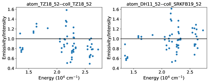
Figure 7: Ratio of the normalized theoretical emissivity and observed intensity for lines in HH 202S as a function of the upper-level energy of the transition. Left panel: spectral fit with datasets atom_TZ18_52 and coll_TZ18_52 at $T_{e}=7.94\times 10^{3}$ K and $n_{e}=3.29\times 10^{4}$ cm^-3. Right panel: spectral fit with datasets atom_DH11_52 and coll_SRKFB19_52 at $T_{e}=11.1\times 10^{3}$ K and $n_{e}=2.58\times 10^{4}$ cm^-3.

In the right panel, the spectral fit was performed with datasets atom_DH11_52 and coll_SRKFB19_52, resulting in a higher temperature $T_{e}=11.1\times 10^{3}$ K and comparable density $n_{e}=2.58\times 10^{4}$ cm^-3; however, the missing continuum-pumping signature is not present. The diverse, high temperatures of Table 11 might thus be interpreted as attempts to fit the spectra without accounting for all the level-populating mechanisms.

A second reading is to look at the critical densities of the levels. In Figure 8, we plot the critical densities at $T_{e}=10^{4}$ K for the lower 52 levels of [Fe ii] computed with dataset atom_TZ18_52 and three coll files: B15_52, SRKFB19_52, and TZ18_52. For levels with index $i>10$, critical densities by coll_B15_52 are a factor of two higher, and for $i>35$, they are all significantly different from each other. A key feature is the low critical density ($\log\rho_{\mathrm{crit}}<2.6$) of the $\mathrm{3d^{7}\ a\,^{4}F_{9/2}}$ metastable level (level $i=6$). For an electron density $n_{e}=2\times 10^{4}$ cm^-3, the population of this level may be larger than that of the ground level for temperatures as low as $T_{e}\approx 7\times 10^{3}$ K; therefore, this level plays a dominant role in the spectral formation of [Fe ii].

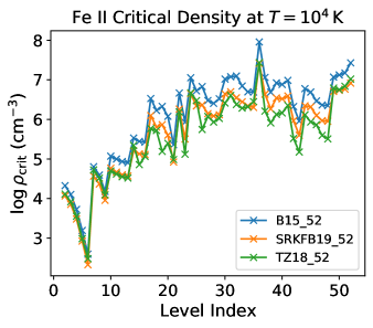
Figure 8: Critical densities for the lower 52 levels of [Fe ii] predicted at $T=10^{4}$ K by using ECS from the coll datasets B15_52, SRKFB19_52, and TZ18_52 and $A$-values from atom_TZ18_52.

Moreover, in Figure 9, we plot the critical density of level $\mathrm{3d^{7}\ a\,^{4}F_{9/2}}$ as a function of temperature using different atomic datasets. In the right panel, we show results computed with the dataset coll_TZ18_52 and three atom files (TZ18_52, B15_52, and DH11_52). Although the sensitivity to the radiative data is extreme, for $T_{e}>5\times 10^{3}$ K, it is approximately temperature independent. In the left panel, the critical density is computed with the atom_TZ18_52 and three coll datasets (B15_52, SRKFB19_52, and TZ18_52). The dependency on the collisional data is not as marked as on the radiative data, but it is temperature dependent.

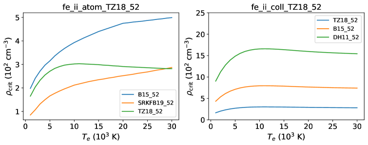
Figure 9: Critical density of level $\mathrm{3d^{7}\ a\,^{4}F_{9/2}}$ of [Fe ii] as a function of temperature computed with different atomic datasets. Left panel: atom_TZ18_52 file and three coll files: B15_52, SRKFB19_52, and TZ18_52. Right panel: coll_TZ18_52 file and three atom files: TZ18_52, B15_52, and DH11_52.

In Table 11, we also list the fit results using the extended dataset pairs atom_TZ18_173–coll_TZ18_173 and atom_TZ18_173–coll_SRKFB19_173. For the HH 202S spectrum, the resulting temperature (in $10^{3}$ K units), density (in $10^{4}$ cm^-3 units), and $\chi^{2}$ values $(T_{e},n_{e},\chi^{2})=(7.81,3.29,7.91)$ and $(T_{e},n_{e},\chi^{2})=(9.75,2.32,2.84)$, respectively, are, as expected, close to those from the atom_TZ18_52–coll_TZ18_52 and atom_TZ18_52–coll_SRKFB19_52 pairs: $(T_{e},n_{e},\chi^{2})=(7.94,3.29,7.90)$ and $(T_{e},n_{e},\chi^{2})=(9.91,2.21,2.75)$. However, for HH 204, the smaller $\chi^{2}$ values in atom_TZ18_173–coll_TZ18_173 and atom_TZ18_173–SRKFB19_173 indicate improved fits: $\chi^{2}=40.2.$ and 64.2 as compared to $\chi^{2}=154.$ and 84.7 in the pairs atom_TZ18_52–coll_TZ18_52 and atom_TZ18_52–coll_SRKFB19_52, respectively. Moreover, although the temperatures and densities with coll_SRKFB19_52 and coll_SRKFB19_173 are close, the densities with coll_TZ18_52 and coll_TZ18_173 differ substantially: 2.63 and 1.51, respectively.

4.3.3 Line-Ratio Diagnostics

An extensive discussion of [Fe ii] line-ratio diagnostics in the infrared, near-infrared, and optical is given in Bautista et al. (2015). Using lines from the HH 202S and HH 204 spectra, we have examined several line ratios to be used as density diagnostics involving “safe” low-energy levels to avoid predicted fluorescence effects Verner et al. (2000). Since temperature diagnostics inherently rely on levels at higher energies, we have refrained from their treatment in the present atomic data comparisons.

We have selected as a showcase in Figure 10 the emissivity ratio $I(\lambda 8892)/I(\lambda 9267)$ that is density sensitive in the range $3\leq\log n_{e}\leq 5$ cm^-3. In the left panel, we plot the emissivity ratio computed with the atom_TZ18_52 radiative dataset and several coll ECS files highlighting its dependency on the collisional datasets. We do not show its behavior below $\log n_{e}=3$ as it becomes more complicated, manifesting divergences also due to the radiative data. We also include in Figure 10 the observed intensity ratio in HH 202S, $I(\lambda 8892)/I(\lambda 9267)=2.36\pm 0.42$, which, except for the curve computed with coll_TZ18_52 ECS, seems to degrade the diagnostic potential of this ratio for $\log n_{e}\gtrapprox 4.5$ since the density variations lie within its error band. On the other hand, the temperature dependency of the ratio above $T_{e}\approx 10^{4}$ K is generally weak, as shown in the right panel.

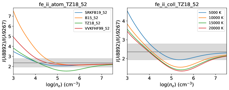
Figure 10: Density behavior of the [Fe ii] $I(\lambda 8892)/I(\lambda 9267)$ emissivity ratio using different atomic datasets. The observed ratio in HH 202S is $2.36\pm 0.42$, which is depicted as a gray band. Left panel: atom_TZ18_52 radiative dataset with four coll datasets (SRKFB19_52, B15_52, TZ18_52, VVKFHF99_52) at $T_{e}=10^{4}$ K. Right panel: atom_TZ18_52 and coll_TZ18_52 datasets at four electron temperatures.

If this observed line-intensity ratio in HH 202S is used to determine the density, we obtain $7.94\times 10^{4}$, $1.32\times 10^{4}$, $1.41\times 10^{4}$, and $3.55\times 10^{4}$ cm^-3 for the coll datasets B15_52, TZ18_52, SRKFB19_52, and VVKFHF99_52, respectively, which compare poorly with estimates from the spectrum fits of Section 4.3.2: respectively, $5.98\times 10^{4}$, $3.29\times 10^{4}$, $2.21\times 10^{4}$, and  $1.47\times 10^{4}$ cm^-3. Nonetheless, if we take into consideration the gross uncertainties brought about by the collisional datasets, on average, both methods coincide on a similar poor density diagnostic: $(4\pm 3)\times 10^{4}$ cm^-3.

4.4 Radiative Lifetimes of the $\mathrm{3d^{6}4s}$, $\mathrm{3d^{7}}$, and $\mathrm{3d^{5}4s^{2}}$ Levels

To compare the lifetimes of levels belonging to the $\mathrm{3d^{6}4s}$, $\mathrm{3d^{7}}$, and $\mathrm{3d^{5}4s^{2}}$ configurations predicted by the atom datasets B15_52, DH11_52, TZ18_52, SRKFB19_52, QDZa96, and QDZh96, we again determine an average lifetime for each level by comparing the respective differences for each dataset (see Figure 11). A problematic and identifiable case in this plot is the lowest level of the first excited configuration, $\mathrm{3d^{7}\ a\,^{4}F_{9/2}}$, with the longest lifetime ($\log\overline{\tau}=4.22$ s) and large discrepant values ($\sim 0.4$ dex). This is an important metastable level inasmuch as being dominant in the plasma radiative and collisional equilibrium and in opening the routes to continuum pumping. In general, the scatter is $\sim 0.1$ dex, except for lifetimes derived from the $A$-values of the questionable atom_SRKB19_52 dataset.

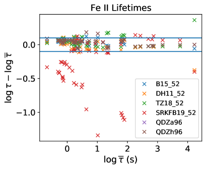
Figure 11: [Fe ii] radiative lifetimes for levels within the $\mathrm{3d^{6}4s}$, $\mathrm{3d^{7}}$, and $\mathrm{3d^{5}4s^{2}}$ configurations computed from the $A$-values in the atom datasets B15_52, DH11_52, TZ18_52, SRKFB19_52, QDZa96, and QDZh96. For each level, the lifetime differences for these datasets with respect to the average value are plotted as a function of the average value.

Lifetimes for a handful of metastable levels of [Fe ii] have been measured with a laser probing technique, and $A$-values were derived using branching fractions from the spectra of the Eta Carinae ejecta taken with the Hubble Space Telescope Rostohar et al. (2001); Hartman et al. (2003); Gurell et al. (2009). A comparison between the experimental lifetimes and those derived from the PyNeb atom datasets is given in Table 12. Lifetimes from atom_SRKFB19_52 are markedly discrepant from both the measured and other theoretical values and are thus excluded from this table. The theoretical lifetime of the $\mathrm{3d^{6}4s\ b\,^{2}H_{11/2}}$ level shows a large scatter. Although there is good agreement between theory and experiment for the $\mathrm{3d^{5}4s^{2}\ a\,^{6}S_{5/2}}$ level, the rest of the lifetimes from B15_52, DH11_52, and TZ18_52 are generally longer (as long as 33%) than experiment. The best overall agreement with the experiment ($\lesssim 7\%$) is displayed by atom_QDZh96. In Table 13, we compare experimental and theoretical $A$-values. QDZh96 values are within the experimental error bars except for $A(\mathrm{a\,^{4}G_{9/2},a\,^{4}F_{9/2}})$ and $A(\mathrm{b\,^{4}D_{7/2},a\,^{4}F_{7/2}})$ for which the theoretical $A$-values agree to within 12%. The average agreement between the experiment and the rest of the theoretical data is around 20%.

4.5 Radiative Lifetimes of the $\mathrm{3d^{6}(^{5}D)4p}$ Odd-Parity Levels

Radiative lifetimes of the Fe ii odd-parity levels $\mathrm{3d^{6}(^{5}D)4p}$ have been measured with a time-resolved non-linear laser-induced fluorescence technique, whereby an improved signal-to-noise ratio reduces uncertainties to 2–3% Schnabel et al. (2004). In Table 14, we compare these measurements with lifetimes derived from $A$-values from atom_TZ18_173 and atom_RKFB19_173. Theoretical lifetimes agree to $\sim 30\%$ but are, on average, around 14% shorter than measurements and well outside the aforementioned error bars.

Table 12: Comparison of [Fe ii] experimental lifetimes (in s) with those derived from the revised PyNeb atom datasets. The error of the least significant figure of the observed lifetime is indicated in brackets.

	Experiment			Theory
Level	Ref. Rostohar et al. (2001)	Ref. Hartman et al. (2003)	Ref. Gurell et al. (2009)	B15_52	DH11_52	TZ18_52	QDZa96	QDZh96
$\mathrm{3d^{5}4s^{2}\ a\,^{6}S_{5/2}}$	0.23(3)			0.241	0.233	0.225	0.262	0.220
$\mathrm{3d^{6}4s\ a\,^{4}G_{11/2}}$			0.75(10)	0.909	0.960	0.934	0.774	0.706
$\mathrm{3d^{6}4s\ a\,^{4}G_{9/2}}$		0.65(2)		0.849	0.862	0.876	0.755	0.694
$\mathrm{3d^{6}4s\ b\,^{2}H_{11/2}}$		3.8(3)		5.31	3.71	4.18	6.59	5.20
$\mathrm{3d^{6}4s\ b\,^{4}D_{1/2}}$			0.54(3)	0.592	0.627	0.632	0.616	0.550
$\mathrm{3d^{6}4s\ b\,^{4}D_{7/2}}$	0.53(3)			0.548	0.578	0.575	0.568	0.501

Table 13: Comparison of experimental $A$-values (s^-1) for transitions in [Fe ii] with those listed in the revised PyNeb atom datasets. The error of the least significant figure of the observed $A$-value is indicated in brackets.

			Experiment		Theory
Upper	Lower	$\lambda_{\mathrm{air}}$ (Å)	Ref. Hartman et al. (2003)	Ref. Gurell et al. (2009)	B15_52	DH11_52	TZ18_52	QDZa96	QDZh96
$\mathrm{a\,^{4}G_{9/2}}$	$\mathrm{a\,^{4}F_{9/2}}$	4177.20	0.29(5)		0.16	0.14	0.14	0.18	0.19
	$\mathrm{a\,^{4}F_{7/2}}$	4276.84	0.83(7)		0.66	0.65	0.65	0.75	0.82
	$\mathrm{a\,^{4}F_{5/2}}$	4352.78	0.36(4)		0.31	0.31	0.29	0.35	0.38
$\mathrm{a\,^{6}S_{5/2}}$	$\mathrm{a\,^{6}D_{9/2}}$	4287.39	1.53(22)		1.50	1.55	1.62	1.37	1.65
	$\mathrm{a\,^{6}D_{7/2}}$	4359.33	1.19(21)		1.11	1.15	1.19	1.02	1.22
	$\mathrm{a\,^{6}D_{5/2}}$	4413.78	0.84(13)		0.78	0.81	0.84	0.73	0.86
	$\mathrm{a\,^{6}D_{3/2}}$	4452.10	0.53(8)		0.50	0.52	0.54	0.47	0.55
	$\mathrm{a\,^{6}D_{1/2}}$	4474.90	0.26(4)		0.24	0.25	0.26	0.23	0.27
$\mathrm{b\,^{4}D_{7/2}}$	$\mathrm{a\,^{6}D_{9/2}}$	3175.38	0.23(3)		0.21	0.24	0.21	0.19	0.21
	$\mathrm{a\,^{4}F_{9/2}}$	3376.20	0.96(10)		0.88	0.77	0.81	0.85	0.98
	$\mathrm{a\,^{4}F_{7/2}}$	3440.99	0.23(3)		0.30	0.27	0.28	0.29	0.33
	$\mathrm{a\,^{4}P_{5/2}}$	5551.31	0.18(4)		0.15	0.14	0.14	0.15	0.18
	$\mathrm{a\,^{4}P_{3/2}}$	5613.27	0.10(3)		0.078	0.069	0.075	0.081	0.093
$\mathrm{a\,^{4}G_{11/2}}$	$\mathrm{a\,^{4}F_{9/2}}$	4243.97		1.05(15)	0.85	0.81	0.84	1.02	1.12
	$\mathrm{a\,^{4}F_{7/2}}$	4346.85		0.25(5)	0.20	0.18	0.18	0.23	0.25

Experimental E1 $A$-values were reported using the lifetimes in Table 14 and branching fractions determined with a Fourier transform spectrometer and a high-resolution grating spectrometer to precisions of 6% and 26% for the strong and weak transitions, respectively Schnabel et al. (2004). We compare these measurements with $A$-values from atom_TZ18_173 and atom_SRKFB19_173 in Figure 12. $A$-values from the former dataset with $\log A>6$ agree with the experiment to within 0.3 dex, while large discrepancies (as large as 3 dex) are displayed by the latter.

4.6 Fe ii $gf$-Values

Oscillator strengths ($gf$-values) for 142 Fe ii lines ($\lambda\lambda 4000{-}8000$) have been derived from both laboratory and computed data and benchmarked with accurate spectra from the Sun and metal-poor stars Meléndez and Barbuy (2009). These $gf$-values have been compared with data computed with extensive CI using the mcbp code civ3, including fine-tuning Deb and Hibbert (2014). This calculation included 262 fine-structure levels from the $\mathrm{3d^{6}4s}$, $\mathrm{3d^{7}}$, $\mathrm{3d^{5}4s^{2}}$, $\mathrm{3d^{6}4p}$, and $\mathrm{3d^{5}4s4p}$ configurations. In general, good agreement was found except for a few ill-behaved transitions susceptible to effects difficult to constrain computationally such as severe cancellation due to CI mixing.

Table 14: Comparison of experimental lifetimes (in ns) of the $\mathrm{3d^{6}(^{5}D)4p}$ levels of Fe ii with those derived from $A$-values listed in the revised PyNeb atom datasets. The error of the least significant figure of the observed lifetime is indicated in brackets.

	Experiment	Theory
Level	Ref. Schnabel et al. (2004)	TZ18_173	SRKFB19_173
$\mathrm{z\,^{6}D^{o}_{9/2}}$	3.68(7)	3.17	3.39
$\mathrm{z\,^{6}D^{o}_{7/2}}$	3.67(9)	3.19	3.43
$\mathrm{z\,^{6}D^{o}_{5/2}}$	3.69(5)	3.20	3.44
$\mathrm{z\,^{6}D^{o}_{3/2}}$	3.73(7)	3.21	3.44
$\mathrm{z\,^{6}D^{o}_{1/2}}$	3.68(11)	3.21	3.45
$\mathrm{z\,^{6}F^{o}_{11/2}}$	3.20(5)	2.58	2.94
$\mathrm{z\,^{6}F^{o}_{9/2}}$	3.28(4)	2.63	2.98
$\mathrm{z\,^{6}F^{o}_{7/2}}$	3.25(6)	2.65	3.09
$\mathrm{z\,^{6}F^{o}_{5/2}}$	3.30(5)	2.66	3.03
$\mathrm{z\,^{6}F^{o}_{3/2}}$	3.45(12)	2.67	3.04
$\mathrm{z\,^{6}P^{o}_{7/2}}$	3.71(4)	2.93	3.53
$\mathrm{z\,^{6}P^{o}_{5/2}}$	3.75(10)	2.91	3.60
$\mathrm{z\,^{6}P^{o}_{3/2}}$	3.70(12)	2.89	3.57
$\mathrm{z\,^{4}D^{o}_{7/2}}$	2.97(4)	2.74	2.10
$\mathrm{z\,^{4}D^{o}_{5/2}}$	2.90(6)	2.76	2.15
$\mathrm{z\,^{4}D^{o}_{3/2}}$	2.91(9)	2.74	2.13
$\mathrm{z\,^{4}F^{o}_{9/2}}$	3.72(10)	3.29	3.14
$\mathrm{z\,^{4}F^{o}_{7/2}}$	3.59(10)	3.14	3.00
$\mathrm{z\,^{4}F^{o}_{5/2}}$	3.55(8)	3.16	2.99
$\mathrm{z\,^{4}P^{o}_{5/2}}$	3.27(6)	3.20	2.74
$\mathrm{z\,^{4}P^{o}_{3/2}}$	3.23(9)	3.21	2.55

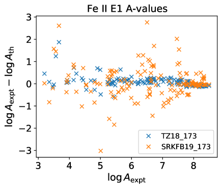
Figure 12: Comparison of experimental $A$-values (s^-1) for E1 transitions arising from the $\mathrm{3d^{6}(^{5}D)4p}$ levels of Fe ii Schnabel et al. (2004) with those from the atom datasets TZ18_173 and SRKFB19_173.

In Figure 13, we compare the observed $gf$-values (MB09) Meléndez and Barbuy (2009) with theoretical data from Ref. Deb and Hibbert (2014) (DH14), atom_TZ18_173, and atom_SRKFB19_173. If problematic transitions are excluded, the average agreement of DH14 and atom_TZ18_173 with MB09 is within 0.2 dex. Dataset atom_SRKFB19_173, on the other hand, contains several transitions with discrepancies greater than 0.5 dex.

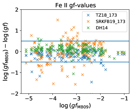
Figure 13: Comparison of observed $gf$-values for Fe ii (MB09) Meléndez and Barbuy (2009) with those calculated from atom_TZ18_173, atom_SRKFB19_173, and Ref. Deb and Hibbert (2014) (DH14).

Table 15 shows three transitions for which DH14 shows sizable discrepancies with respect to MB09. Datasets atom_TZ18_173 and atom_SRKFB19_173 do not perform much better; thus, the hindrance from cancellation effects in computational estimates put forward in Ref. Deb and Hibbert (2014) is reinforced. This table also lists three transitions we were not able to identify in atom_TZ18_173 or atom_SRKFB19_173 for which the agreement between DH14 and MB09 is reasonable.

Table 15: Problematic transitions in the $gf$-value comparison of MB09 Meléndez and Barbuy (2009) with atom_TZ18_173, atom_SRKFB19_173, and DH14 Deb and Hibbert (2014) showing large discrepancies or unidentified lines.

			MB09	TZ18_173	SRKFB19_173	DH14
Lower	Upper	$\lambda_{\mathrm{air}}$ (Å)	$\log(gf)$
$\mathrm{3d^{6}4p\ z\,^{4}F^{o}_{5/2}}$	$\mathrm{3d^{5}4s^{2}\ c\,^{4}D_{3/2}}$	6508.13	$-$3.45	$-$3.93	$-$2.56	$-$7.90
$\mathrm{3d^{6}4s\ c\,^{4}F_{9/2}}$	$\mathrm{3d^{6}4p\ x\,^{4}G^{o}_{9/2}}$	6433.81	$-$2.37	$-$3.82	$-$2.91	$-$4.41
$\mathrm{3d^{6}4p\ z\,^{4}F^{o}_{7/2}}$	$\mathrm{3d^{5}4s^{2}\ c\,^{4}D_{5/2}}$	6371.13	$-$3.13	$-$3.54	$-$2.48	$-$4.19
		4635.32	$-$1.42			$-$1.75
		4625.89	$-$2.35			$-$2.41
		4549.19	$-$1.62			$-$1.86

4.7 Fe ii Branching Fractions

Branching fractions

$$BF_{ji}=\frac{I(j,i)}{\sum_{i}I(j,i)}=\frac{A(j,i)}{\sum_{i}A(j,i)}$$ (4)

for 121 Fe ii UV lines originating from levels of the $\mathrm{3d^{6}(^{5}D)4p}$ configuration have been measured in low-current spectra from Fe–Ne and Fe–Ar hollow cathode discharge lamps. The spectra were taken with a UW 3 m echelle spectrograph with a resolving power of 250,000 Den Hartog et al. (2019). We compare these branching fractions in Figure 14 with those derived from $A$-values of the atom_TZ18_173 and atom_SRKFB19_173 atom datasets. For transitions with $\log(BF_{\mathrm{expt}})>-2$, the branching fractions from atom_TZ18_173 agree with the experiment, on average, to better than 30%, while significantly larger discrepancies are displayed by atom_SRKFB19_173. However, most theoretical branching fractions, in general, do not match the accuracy implicit in the experimental error bars.

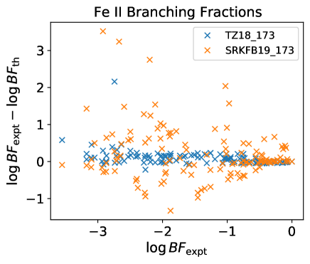
Figure 14: Comparison of Fe ii experimental branching fractions ($BF_{\mathrm{expt}}$) Den Hartog et al. (2019) with theoretical values ($BF_{\mathrm{th}}$) derived from atom_TZ18_173 and atom_SRKFB19_173.

4.8 [Fe ii] Effective Collision Strengths

We have constructed three revised coll datasets containing ECS for the [Fe ii] 52-level atomic model of PyNeb: B15_52, TZ18_52, and SRKFB19_52. We determine for each transition the average ECS from these three datasets at $T=10^{4}$ K, and as depicted in Figure 15, we compare the logarithmic differences with respect to this average. ECS from coll_B15_52 appear to lie below average, displaying differences as large as $\Delta\log\Upsilon\approx-4$, while those from coll_SRKFB19_52 are above average with a scatter within 1.0 dex. The most interesting result is coll_TZ18_52 with an ECS average well within 0.5 dex. This outcome supports the findings in the spectrum fits (see Table 11), whereby the electron densities predicted by coll_B15_52 are higher, coll_SRKFB19_52 lower, and coll_TZ18_52 in between.

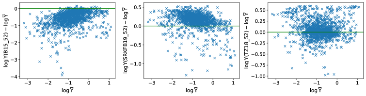
Figure 15: [Fe ii] ECS logarithmic differences at $T=10^{4}$ K for each transition in the coll datasets B15_52, SRKFB19_52, and TZ18_52 relative to the average value.

Due to the diagnostic potential of [Fe ii] emission lines in interstellar-medium plasmas, accurate ECS at low temperatures were recently computed for transitions among levels of the $\mathrm{3d^{6}(^{5}D)4s\ a\,^{6}D}_{J}$ ground term Wan et al. (2019). To obtain uncertainty estimates, different target models and relativistic $R$-matrix methods (bprm, icft, darc) were used in these calculations. In Figure 16, we compare selected ECS from Wan et al. (2019) with those from coll datasets B15_52, TZ18_52, and SRKFB19_52. For this purpose, we use the PyNeb getOmega(T,j,i) function that allows ECS linear interpolation at the input temperature T; if the latter lies outside the temperature range of the tabulated ECS, the function lists the end value. This is the case of coll_B15_52 and coll_SRKFB19_52 for $\log T<3$ (see Figure 16). As expected, the best agreement is with coll_SRKFB19_52, although there are points outside the error bars. Large discrepancies are also found with coll_B15_52 and coll_TZ18_52 at higher temperatures ($\log T>4$).

Figure 16: ECS $\Upsilon(J-J^{\prime})$ for the transitions $\mathrm{3d^{6}(^{5}D)4s\ a\,^{6}D}_{J}-\mathrm{a\,^{6}D}_{J^{\prime}}$ within the ground term of [Fe ii]. Blue circles: Ref. Wan et al. (2019). Yellow crosses: coll_B15_52. Green squares: coll_SRKFB19_52. Red triangles: coll_TZ18_52.

4.9 Fe ii Discussion

In the implementation of new datasets for [Fe ii], we found term misassignments for levels with total orbital angular momentum quantum number $L=5$ in the atomic model of atom_SRKFB19_225 (see Table 6). A further comparison in Table 7 of $A$-values for transitions arising from the $\mathrm{3d^{6}4s\ a\,^{4}H_{J}}$ and $\mathrm{3d^{6}4s\ b\,^{2}H_{J}}$ ($J=9/2$ and $11/2$) levels indicate large discrepancies with respect to other atom datasets (TZ18_225, DH11_52, B15_52, QDZa96, and QDZh96). This is an indication of faulty data that can be corroborated with the discrepancies displayed by dataset atom_SRKFB19_52 in the comparison of observed and computed $A$-value ratios carried out in Section 4.3.1.

This comparison also brings out observed lines with questionable identifications (e.g., $\lambda\lambda 3968.27,4889.71$) and unreliable line-intensity ratios—e.g., $I(\lambda 7637.52)/I(\lambda 9051.95)$, $I(\lambda 7686.93)/\allowbreak I(\lambda 8891.93)$, and $I(\lambda 7733.13)/I(\lambda 9033.49)$—due to $A$-values with magnitude $\log A\lesssim-3$. Theoretical $A$-value ratios agree to within 20–25% and, with respect to the observed line-intensity ratios, to within the error bars except for some outliers subject to strong level mixing, as pointed out in Deb and Hibbert (2010a).

We have found atomic data files, namely atom_B15 and coll_B15, with faulty data caused again by the incorrect mapping to atomic models with different level numbering. This problem is exacerbated by data producers who use several multi-configuration methods implementing a variety of relativistic Hamiltonians (Dirac–Fock, Breit–Pauili, Pauli). This multi-code approach may enable accuracy estimates of the radiative and collisional data, but it often leads to level structures with conflicting numbering and identifications that are difficult to remap. The use of fine-tuning in atomic calculations to match the experimental level order does mitigate this problem.

In contrast to [Fe iii], for which the spectrum fits using different atomic datasets resulted in acceptable temperature (6%) and density (20%) uncertainties thus sustaining their reliability, for [Fe ii], the collisional datasets lead to temperature variations of around 15–20% and density discrepancies as large as a factor of four. However, the reasonable temperature and density accord between coll_SRKFB19_52 and coll_VVKFHF99_52 must be noted. These results appear to indicate that, for [Fe ii], the electron density is not a good fitting parameter or, as previously proposed Rodríguez (1999); Verner et al. (2000); Hartman (2013), fluorescence continuum pumping might be a level-populating mechanism we have not taken into account. Furthermore, the extremely low critical density of level $\mathrm{3d^{7}\ a\,^{4}F_{9/2}}$ (see Figure 8) and its sensitivity to both the radiative and collisional datasets (Figure 9) give this level a protagonistic role in the [Fe ii] spectrum formation, notwithstanding the poor accuracy of its small $A$-value.

The potential of line-ratio density diagnostics in [Fe ii] is compromised by the mismatch with the spectrum fits, and the temperature diagnostics are discouraged by the looming role of fluorescence pumping. In Section 4.3.3, we use the $I(\lambda 8892)/I(\lambda 9267)$ ratio to illustrate a density diagnostic problem: the density variations in the range of interest ($3\leq\log n_{e}\leq 5$ cm^-3) lie within the observed line-intensity error band. As performed in Section 3.3.3 for the analysis of the [Fe iii] density diagnostics, an observational sample of low-density ionized nebulae with [Fe ii] detections would be helpful to constrain the predictions of both the radiative and collisional parameters. The lack of such a sample in the literature prevents us from drawing further conclusions.

We have performed extensive comparisons of computed and measured radiative data for both the $\mathrm{3d^{6}4s}$, $\mathrm{3d^{7}}$, and $\mathrm{3d^{5}4s^{2}}$ even-parity levels and the $\mathrm{3d^{6}4p}$ and $\mathrm{3d^{5}4s4p}$ odd-parity levels. Regarding even-parity levels (see Section 4.4), the computed radiative lifetimes agree to within 0.1 dex except for the singular $\mathrm{3d^{7}\ a\,^{4}F_{9/2}}$ metastable level with $\log\tau\sim 4$ s and an uncertainty of 0.4 dex. It must be noted that the $A$-values in atom_SRKB19_52 display questionable lifetimes for some of these levels (see Figure 11). The best overall agreement between theory and experiment ($\sim 7\%$) is with the atom_QDZh96 dataset, while other atom datasets (B15_52, DH11_52, and TZ18_52) in general yield longer (as long as 33%) lifetimes than experiment. As discussed in Deb and Hibbert (2010a), the large uncertainty of the $\mathrm{3d^{6}4s\ b\,^{2}H_{11/2}}$ lifetime is caused by imprecise level mixing. $A$-values derived from the experimental lifetimes, on average, agree to around 20% with those in the theoretical datasets.

Accurate (2–3%) radiative lifetimes have been measured for the $\mathrm{3d^{6}(^{5}D)4p}$ odd-parity levels Schnabel et al. (2004), which have been compared in Section 4.5 with those derived from the atom_TZ18_173 and atom_SRKFB19_173 datasets. Theoretical lifetimes agree to within 30%, but on average they are around 14% shorter than measurements. E1 $A$-values have also been derived from these lifetime measurements, and those with $\log A>6$ agree with atom_TZ18_173 to within 0.3 dex while larger discrepancies (as large as 3 dex) are found in atom_SRKFB19_173. Moreover, the comparison of the observed $gf$-values Meléndez and Barbuy (2009) in Section 4.6 with those derived from the theoretical datasets shows good agreement (0.2 dex) with atom_TZ18_173 and discrepancies larger than 0.5 dex with atom_SRKFB19_173. A similar outcome is obtained in the comparison of measured branching ratios Den Hartog et al. (2019) in Section 4.7, whereby those derived from $A$-values in atom_TZ18_173 with $\log(BF_{\mathrm{expt}})>-2$ agree to better than 30%, while some from atom_SRKFB19_173 show larger discrepancies. In general, the theoretical radiative datasets do not reach anywhere near the accuracy quoted for the measured lifetimes, $A$-values, $gf$-values, and branching fractions.

The comparison of collisional datasets in Figure 15 of Section 4.8 gives a macro-measure of the overall ECS magnitudes that has a direct impact on the critical densities. In this comparison, we determined for each transition an average ECS using three coll datasets (B15_52, SRKFB19_52, and TZ18_52) and then plotted the dispersion for each dataset. Figure 15 shows that the smallest dispersion (within 0.5 dex) is by coll_TZ18_52 while differences in coll_B15_52 and coll_SRKFB19_52 are larger and, respectively, mostly negative and positive. The fairly large ECS discrepancies found in Figure 16 for transitions within the $\mathrm{3d^{6}(^{5}D)4s\ a\,^{6}D}$ ground term at low temperatures gives a further indication of the patchy quality of the collisional data for Fe ii.

From the extensive data tests hereby carried out on the Fe ii datasets, we find the radiative data in atom_SRKFB19_52 to be faulty, and this could indeed have an impact on the coll_SRKFB19_52 data. We would therefore select as the PyNeb 1.1.17 defaults the atom_TZ18_173 and coll_ TZ18_173 datasets.

5 Conclusions

We have performed extensive data evaluations of the levels, atom, and coll files for [Fe iii] and [Fe ii] in PyNeb 1.1.16 to examine their worthiness in nebular spectral modeling and to select the package defaults. In most cases, we have reconstructed the datasets from the sources and introduced newly published data, thus leading to a more reliable atomic database for these species in the new release PyNeb 1.1.17.

The present data assessment comprises: fits of high-resolution spectra from the HH 202S and HH 204 Herbig–Haro objects taken with the Ultraviolet Visual Echelle Spectrograph Mesa-Delgado et al. (2009); Méndez-Delgado et al. (2021b); comparisons of theoretical and observed line-intensity ratios; and comparisons with measurements of radiative lifetimes, $A$-values, $gf$-values, and branching ratios. Observed lines may suffer from misidentifications, line blending, and telluric or instrumental contamination. On the other hand, the computation of accurate radiative data for lowly ionized ions of the iron group with open $\mathrm{3d}^{n}$ shells is hindered by strong configuration mixing, double-excitation representations, and subtle core–valence correlation involving closed and open subshells; thus, broadly speaking, we would not expect an $A$-value accuracy of better than 20%. Similarly, the ECS at low temperatures are affected by complex resonance structures sensitive to target models and channel convergence that seriously compromise accuracy ratings.

For Fe iii, we introduced a new levels file from the NIST database with more complete level assignments and accurate energies. The previous version of the levels file is in the deprecated directory, renamed as fe_iii_levels_2023.dat. As described in Section 3.2, we implemented the new atom files Q96_34, DH09_34, BBQ10_34, BB14_34, and BB14_144 and the coll files Z96_34, BBQ10_34, BB14_34, Z96_144, and BB14_144. In PyNeb 1.1.17 atom_BBQ10_34, atom_BB14_34, coll_Z96_34 are not included as they are, respectively, made redundant by atom_BBQ10, atom_BB14_144, and coll_Z96_144 while coll_BB14 and coll_BBQ10 are deprecated.

A comparison of the observed line-intensity ratios for transitions arising from the same upper level in [Fe iii] with the corresponding $A$-value ratios constrains the overall accuracy of the latter to around 20–30%. Spectrum fits with the new datasets led to temperatures and densities within 6% and 20%, respectively, validating their usefulness. Radiative lifetimes computed with these atom datasets agree to within 0.1 dex. A revision of coll files brings out the incompleteness of the Z96_34 dataset and its poor accuracy for ECS with $\log\Upsilon<-1$. For [Fe iii], we have selected the atom_BB14_144 and coll_BB14_144 datasets as the defaults in PyNeb 1.1.17.

For Fe ii, we have implemented the atom files VVKFHF99_52, DH11_52, B15_52, TZ18_52, SRKFB19_52, TZ18_173, SRKFB19_173 and coll files VVKFHF99_52, B15_52, TZ18_52, SRKFB19_52, TZ18_173, and SRKFB19_173. After extensive tests and much pondering, the atom_SRKFB19_52 and atom_SRKFB19_173 datasets were found to contain faulty $A$-values, while atom_VVKFHF99_52 and coll_VVKFHF99_52 have missing data; therefore, these files are not included in PyNeb 1.1.17. Apart from this drawback, the theoretical $A$-value ratios for transitions arising from a common upper level derived from the rest of the atom files agree to within 20–25%, and most lie within the experimental error bars. The spectrum fits yielded temperature and density variations of around 20% and a factor of 4, respectively, which appear to indicate that the density is not a good fitting parameter and fluorescence continuum pumping might be a level-populating contributor not taken into account. However, the poor theoretical characterization of the key level $\mathrm{3d^{7}\ a\,^{4}F_{9/2}}$, inasmuch as its inaccurate $A$-value and extremely low critical density sensitive to both the radiative and collisional datasets, deters us from more conclusive remarks. Extensive comparisons of the radiative data for both forbidden and allowed transitions with experiment bring out the computational difficulties to match the measured accuracy (better than 10%); thus, a global theoretical $A$-value accuracy of 20–30% would be statistically sound. Finally, the examined coll datasets lead to different critical densities around $T_{e}=10^{4}$ K, a situation that is difficult  to analyze.

In PyNeb 1.1.17, the atom files VVKFHF99_52, TZ18_52 and coll files VVKFHF99_52, SRKFB19_52, SRKFB19_173 are made redundant by atom_VVKFHF99, atom_TZ18_173,
coll_VVKFHF99, and coll_SRKFB19. Furthermore, atom_B15, coll_B15, atom_VVKFHF99, coll_VVKFHF99 are deprecated. We select atom_TZ18_173 and coll_TZ18_173 as defaults.

The status of all the data files for Fe iii and Fe ii in PyNeb 1.1.16 and 1.1.17 are summarized in Table 16 of Appendix A.

A final recommendation emerging from the present work must be put forward regarding the curation of the atomic databases associated with spectral modeling codes. The potential of the latter in astrophysical analyses relies in great part on the integrity (accuracy and completeness) of their tabulations of radiative and collisional rates, which, as shown here, demand detailed evaluation and upgrading. For complex ionic spectra such as [Fe iii] and [Fe ii], this may imply a lengthy endeavor.

C.M. (Claudio Mendoza) conceptualized and coordinated the full paper. J.E.M.-D. and J.G.-R. provided the observational data and extensive discussions about their validity and provenance. M.A.B. provided data, performed calculations, and led discussions about fluorescence continuum pumping in [Fe ii]. C.M. (Christophe Morisset) researched data, performed ancillary calculations, and software support regarding the PyNeb package. Investigation, methodology, analysis, and validation: C.M. (Claudio Mendoza), J.E.M.-D., J.G.-R., M.A.B., C.M. (Christophe Morisset). Writing and original draft preparation: C.M. (Claudio Mendoza), J.E.M.-D. Review and editing: C.M. (Claudio Mendoza), J.E.M.-D., C.M. (Christophe Morisset), J.G.-R., M.A.B. Visualization: C.M. (Claudio Mendoza), J.E.M.-D. All authors have read and agreed to the published version of the manuscript.

J.E.M.-D. acknowledges funding from the Deutsche Forschungsgemeinschaft (DFG, German Research Foundation) in the form of an Emmy Noether Research Group (grant number KR4598/2-1, PI Kathryn Kreckel). Ch.M. acknowledges the support from UNAM/DGAPA/PAPIIT grant IN101220. J.G.-R. acknowledges support from an Advanced Fellowship under the Severo Ochoa excellence program CEX2019-000920-S; financial support from the Canarian Agency for Research, Innovation, and Information Society (ACIISI) of the Canary Islands Government and the European Regional Development Fund (ERDF) under grant with reference ProID2021010074; and support under grant P/308614 financed by funds transferred from the Spanish Ministry of Science, Innovation, and Universities (MCIU) charged to the General State Budgets and with funds transferred from the General Budgets of the Autonomous Community of the Canary Islands by the MCIU.

The data files revised and compiled for this revision are publicly available in PyNeb 1.1.17.

Appendix A

Table 16: Status of the Fe iii and Fe ii atomic data files in the PyNeb library for versions 1.1.16 and 1.1.17. ‘X’ means the file is present; ‘*’ means the file is present and is the default; ‘D’ means the file is deprecated (but may still be accessible with the command pn.atomicData.includeDeprecatedPath()).

Fe iii File Name	v1.1.16	v1.1.17	Fe ii File Name	v1.1.16	v1.1.17
fe_iii_atom_BB14_144.dat		*	fe_ii_atom_TZ18_173.dat		*
fe_iii_atom_BBQ10.dat	X	X	fe_ii_atom_B15.dat	*	D
fe_iii_atom_DH09_34.dat		X	fe_ii_atom_B15_52.dat		X
fe_iii_atom_NP96.dat	X	X	fe_ii_atom_DH11_52.dat		X
fe_iii_atom_Q96_34.dat		X	fe_ii_atom_SRKFB19.dat	X	D
fe_iii_atom_Q96_J00.dat	*	X	fe_ii_atom_VVKFHF99.dat	X	D
fe_iii_coll_BB14_144.dat		*	fe_ii_coll_TZ18_173.dat		*
fe_iii_coll_BB14.dat	X	D	fe_ii_coll_B15.dat	*	D
fe_iii_coll_BBQ10.dat	X	D	fe_ii_coll_B15_52.dat		X
fe_iii_coll_BBQ10_34.dat		X	fe_ii_coll_B15_old.dat	X	D
fe_iii_coll_Q96.dat	X	X	fe_ii_coll_SRKFB19.dat	X	X
fe_iii_coll_Z96.dat	*	X	fe_ii_coll_VVKFHF99.dat	X	D
fe_iii_coll_Z96_144.dat		X

[custom]

References

References

- Luridiana et al. (2012) Luridiana, V.; Morisset, C.; Shaw, R.A. PyNeb: A New Software for the Analysis of Emission Lines. In IAU Symposium; Cambridge University Press: Cambridge, UK, 2012; Volume 283, pp. 422–423. https://doi.org/10.1017/S1743921312011738.
- Luridiana et al. (2015) Luridiana, V.; Morisset, C.; Shaw, R.A. PyNeb: A new tool for analyzing emission lines. I. Code description and validation of results. Astron. Astrophys. 2015, 573, A42. https://doi.org/10.1051/0004-6361/201323152.
- Peimbert et al. (2017) Peimbert, M.; Peimbert, A.; Delgado-Inglada, G. Nebular Spectroscopy: A Guide on H II Regions and Planetary Nebulae. Publ. Astron. Soc. Pac. 2017, 129, 082001. https://doi.org/10.1088/1538-3873/aa72c3.
- Morisset et al. (2020) Morisset, C.; Luridiana, V.; García-Rojas, J.; Gómez-Llanos, V.; Bautista, M.; Mendoza.; Claudio. Atomic Data Assessment with PyNeb. Atoms 2020, 8, 66. https://doi.org/10.3390/atoms8040066.
- Juan de Dios and Rodríguez (2021) Juan de Dios, L.; Rodríguez, M. Atomic data and the density structures of planetary nebulae. Mon. Not. R. Astron. Soc. 2021, 507, 5331–5339. https://doi.org/10.1093/mnras/stab2488.
- Perinotto et al. (1999) Perinotto, M.; Bencini, C.G.; Pasquali, A.; Manchado, A.; Rodriguez Espinosa, J.M.; Stanga, R. The iron abundance in four planetary nebulae. Astron. Astrophys. 1999, 347, 967–974.
- Delgado Inglada et al. (2009) Delgado Inglada, G.; Rodríguez, M.; Mampaso, A.; Viironen, K. The Iron Abundance in Galactic Planetary Nebulae. Astrophys. J. 2009, 694, 1335–1348, https://doi.org/10.1088/0004-637X/694/2/1335.
- Delgado-Inglada et al. (2016) Delgado-Inglada, G.; Mesa-Delgado, A.; García-Rojas, J.; Rodríguez, M.; Esteban, C. The Fe/Ni ratio in ionized nebulae: Clues on dust depletion patterns. Mon. Not. R. Astron. Soc. 2016, 456, 3855–3865, https://doi.org/10.1093/mnras/stv2961.
- Mesa-Delgado et al. (2009) Mesa-Delgado, A.; Esteban, C.; García-Rojas, J.; Luridiana, V.; Bautista, M.; Rodríguez, M.; López-Martín, L.; Peimbert, M. Properties of the ionized gas in HH 202—II. Results from echelle spectrophotometry with Ultraviolet Visual Echelle Spectrograph. Mon. Not. R. Astron. Soc. 2009, 395, 855–876, https://doi.org/10.1111/j.1365-2966.2009.14554.x.
- Méndez-Delgado et al. (2021a) Méndez-Delgado, J.E.; Esteban, C.; García-Rojas, J.; Henney, W.J.; Mesa-Delgado, A.; Arellano-Córdova, K.Z. Photoionized Herbig-Haro objects in the Orion Nebula through deep high-spectral resolution spectroscopy—I. HH 529 II and III. Mon. Not. R. Astron. Soc. 2021, 502, 1703–1739, https://doi.org/10.1093/mnras/stab068.
- Méndez-Delgado et al. (2021b) Méndez-Delgado, J.E.; Henney, W.J.; Esteban, C.; García-Rojas, J.; Mesa-Delgado, A.; Arellano-Córdova, K.Z. Photoionized Herbig-Haro Objects in the Orion Nebula through Deep High Spectral Resolution Spectroscopy. II. HH 204. Astrophys J. 2021, 918, 27. https://doi.org/10.3847/1538-4357/ac0cf5.
- D’Odorico et al. (2000) D’Odorico, S.; Cristiani, S.; Dekker, H.; Hill, V.; Kaufer, A.; Kim, T.; Primas, F. Performance of UVES, the echelle spectrograph for the ESO VLT and highlights of the first observations of stars and quasars. In Discoveries and Research Prospects from 8- to 10-Meter-Class Telescopes; Bergeron, J., Ed.; Society of Photo-Optical Instrumentation Engineers (SPIE): Bellingham, WA, USA, 2000; Volume 4005, pp. 121–130. https://doi.org/10.1117/12.390133.
- Garstang (1962) Garstang, R.H. Transition probabilities for forbidden lines of Fe II. Mon. Not. R. Astron. Soc. 1962, 124, 321. https://doi.org/10.1093/mnras/124.4.321.
- Kurucz and Peytremann (1975) Kurucz, R.L.; Peytremann, E. A Table of Semiempirical gf Values. Pt 1: Wavelengths: 5.2682 NM to 272.3380 nm; Pt 2: Wavelengths: 272.3395 NM to 599.3892 nm; Pt 3: Wavelengths: 599.4004 NM to 9997.2746 NM; SAO Special Report; Smithsonian Astrophysical Observatory: Cambridge, MA, USA, 1975.
- Nussbaumer and Storey (1980) Nussbaumer, H.; Storey, P.J. Atomic data for Fe II. Astron. Astrophys. 1980, 89, 308–313.
- Nussbaumer et al. (1981) Nussbaumer, H.; Pettini, M.; Storey, P.J. Sextet transitions in Fe II. Astron. Astrophys. 1981, 102, 351–358.
- Hummer et al. (1993) Hummer, D.G.; Berrington, K.A.; Eissner, W.; Pradhan, A.K.; Saraph, H.E.; Tully, J.A. Atomic data from the IRON project. I. Goals and methods. Astron. Astrophys 1993, 279, 298–309.
- Eissner et al. (1974) Eissner, W.; Jones, M.; Nussbaumer, H. Techniques for the calculation of atomic structures and radiative data including relativistic corrections. Comput. Phys. Commun. 1974, 8, 270–306. https://doi.org/10.1016/0010-4655(74)90019-8.
- Hibbert (1975) Hibbert, A. CIV3—A general program to calculate configuration interaction wave functions and electric-dipole oscillator strengths. Comput. Phys. Commun. 1975, 9, 141–172. https://doi.org/10.1016/0010-4655(75)90103-4.
- Cowan (1981) Cowan, R.D. The Theory of Atomic Structure and Spectra; University of California: Berkeley, CA, USA, 1981.
- Nahar (1995) Nahar, S.N. Atomic data from the Iron Project. VII. Radiative dipole transition probabilities for Fe II. Astron. Astrophys. 1995, 293, 967–977.
- Nahar and Pradhan (1996) Nahar, S.N.; Pradhan, A.K. Atomic data from the Iron Project. XVII. Radiative transition probabilities for dipole allowed and forbidden transitions in Fe III. Astron. Astrophys. Suppl. Ser. 1996, 119, 509–522.
- Quinet et al. (1996) Quinet, P.; Le Dourneuf, M.; Zeippen, C.J. Atomic data from the IRON Project. XIX. Radiative transition probabilities for forbidden lines in Fe II. Astron. Astrophys. Suppl. Ser. 1996, 120, 361–371.
- Zhang and Pradhan (1995) Zhang, H.L.; Pradhan, A.K. Atomic data from the Iron Project. VI. Collision strengths and rate coefficients for Fe II. Astron. Astrophys. 1995, 293, 953–966.
- Zhang (1996) Zhang, H. Atomic data from the Iron Project. XVIII. Electron impact excitation collision strengths and rate coefficients for Fe III. Astron. Astrophys. Suppl. Ser. 1996, 119, 523–528.
- Bautista and Pradhan (1996) Bautista, M.A.; Pradhan, A.K. Atomic data from the Iron project. XIII. Electron excitation rates and emissivity ratios for forbidden transitions in Ni II and Fe II. Astron. Astrophys. Suppl. Ser. 1996, 115, 551–559.
- Bautista et al. (2010) Bautista, M.A.; Ballance, C.P.; Quinet, P. Atomic Data and Spectral Model for Fe III. Astrophys. J. 2010, 718, L189–L193. https://doi.org/10.1088/2041-8205/718/2/L189.
- Badnell and Ballance (2014) Badnell, N.R.; Ballance, C.P. Electron-impact Excitation of Fe2+: A Comparison of Intermediate Coupling Frame Transformation, Breit-Pauli and Dirac R-matrix Calculations. Astrophys. J. 2014, 785, 99. https://doi.org/10.1088/0004-637X/785/2/99.
- Bautista et al. (2015) Bautista, M.A.; Fivet, V.; Ballance, C.; Quinet, P.; Ferland, G.; Mendoza, C.; Kallman, T.R. Atomic Data and Spectral Model for Fe II. Astrophys. J. 2015, 808, 174. https://doi.org/10.1088/0004-637X/808/2/174.
- Tayal and Zatsarinny (2018) Tayal, S.S.; Zatsarinny, O. Electron-impact excitation of forbidden and allowed transitions in Fe II. Phys. Rev. A 2018, 98, 012706. https://doi.org/10.1103/PhysRevA.98.012706.
- Smyth et al. (2019) Smyth, R.T.; Ramsbottom, C.A.; Keenan, F.P.; Ferland, G.J.; Ballance, C.P. Towards converged electron-impact excitation calculations of low-lying transitions in Fe II. Mon. Not. R. Astron. Soc. 2019, 483, 654–663. https://doi.org/10.1093/mnras/sty3198.
- Berrington et al. (1995) Berrington, K.A.; Eissner, W.B.; Norrington, P.H. RMATRX1: Belfast atomic R-matrix codes. Comput. Phys. Commun. 1995, 92, 290–420. https://doi.org/10.1016/0010-4655(95)00123-8.
- Zatsarinny (2006) Zatsarinny, O. BSR: B-spline atomic R-matrix codes. Comput. Phys. Commun. 2006, 174, 273–356. https://doi.org/10.1016/j.cpc.2005.10.006.
- Ait-Tahar et al. (1996) Ait-Tahar, S.; Grant, I.P.; Norrington, P.H. Electron scattering by Fe XXII within the Dirac R-matrix approach. Phys. Rev. A 1996, 54, 3984–3989. https://doi.org/10.1103/PhysRevA.54.3984.
- Griffin et al. (1998) Griffin, D.C.; Badnell, N.R.; Pindzola, M.S. R-matrix electron-impact excitation cross sections in intermediate coupling: An MQDT transformation approach. J. Phys. B At. Mol. Phys. 1998, 31, 3713–3727. https://doi.org/10.1088/0953-4075/31/16/022.
- Wan et al. (2019) Wan, Y.; Favreau, C.; Loch, S.D.; McLaughlin, B.M.; Qi, Y.; Stancil, P.C. Electron-impact fine-structure excitation of Fe II at low temperature. Mon. Not. R. Astron. Soc. 2019, 485, 2252–2258. https://doi.org/10.1093/mnras/stz550.
- Deb and Hibbert (2008) Deb, N.C.; Hibbert, A. Oscillator strengths for transitions among Fe III levels belonging to the three lowest configurations. J. Phys. Conf. Ser. 2008, 130, 012006. https://doi.org/10.1088/1742-6596/130/1/012006.
- Deb and Hibbert (2009a) Deb, N.C.; Hibbert, A. Electric quadrupole and magnetic dipole transitions among 3d6 levels of Fe III. J. Phys. B Atom. Mol. Phys. 2009, 42, 065003. https://doi.org/10.1088/0953-4075/42/6/065003.
- Deb and Hibbert (2009b) Deb, N.C.; Hibbert, A. Weighted f-values, A-values, and line strengths for the E1 transitions among 3d 6, 3d 54s, and 3d 54p levels of Fe III. Atom. Data Nucl. Data Tables. 2009, 95, 184–303. https://doi.org/10.1016/j.adt.2008.12.001.
- Deb and Hibbert (2010a) Deb, N.C.; Hibbert, A. Importance of level mixing on accurate [Fe II] transition rates. Astron. Astrophys. 2010, 524, A54. https://doi.org/10.1051/0004-6361/201015426.
- Deb and Hibbert (2010b) Deb, N.C.; Hibbert, A. Calculation of Intensity Ratios of Observed Infrared [Fe II] Lines. Astrophys. J. 2010, 711, L104–L107. https://doi.org/10.1088/2041-8205/711/2/L104.
- Deb and Hibbert (2011) Deb, N.C.; Hibbert, A. Radiative transition rates for the forbidden lines in Fe II. Astron. Astrophys. 2011, 536, A74. https://doi.org/10.1051/0004-6361/201118059.
- Deb and Hibbert (2014) Deb, N.C.; Hibbert, A. log gf values for astrophysically important transitions Fe II. Astron. Astrophys. 2014, 561, A32. https://doi.org/10.1051/0004-6361/201322751.
- Quinet (1996) Quinet, P. Transition probabilities for forbidden lines of Fe III. Astron. Astrophys. Suppl. Ser. 1996, 116, 573–578.
- Fivet et al. (2016) Fivet, V.; Quinet, P.; Bautista, M.A. Radiative rates for forbidden M1 and E2 transitions of astrophysical interest in doubly ionized iron-peak elements. Astron. Astrophys 2016, 585, A121. https://doi.org/10.1051/0004-6361/201526983.
- Schnabel et al. (2004) Schnabel, R.; Schultz-Johanning, M.; Kock, M. Fe II lifetimes and transition probabilities. Astron. Astrophys. 2004, 414, 1169–1176. https://doi.org/10.1051/0004-6361:20031685.
- Meléndez and Barbuy (2009) Meléndez, J.; Barbuy, B. Both accurate and precise gf-values for Fe II lines. Astron. Astrophys. 2009, 497, 611–617. https://doi.org/10.1051/0004-6361/200811508.
- Den Hartog et al. (2019) Den Hartog, E.A.; Lawler, J.E.; Sneden, C.; Cowan, J.J.; Brukhovesky, A. Atomic Transition Probabilities for UV and Blue Lines of Fe II and Abundance Determinations in the Photospheres of the Sun and Metal-poor Star HD 84937. Astrophys. J. Suppl, Ser. 2019, 243, 33. https://doi.org/10.3847/1538-4365/ab322e.
- Rostohar et al. (2001) Rostohar, D.; Derkatch, A.; Hartman, H.; Johansson, S.; Lundberg, H.; Mannervik, S.; Norlin, L.O.; Royen, P.; Schmitt, A. Lifetime Measurements of Metastable States in Fe+. Phys. Rev. Lett. 2001, 86, 1466–1469. https://doi.org/10.1103/PhysRevLett.86.1466.
- Hartman et al. (2003) Hartman, H.; Derkatch, A.; Donnelly, M.P.; Gull, T.; Hibbert, A.; Johansson, S.; Lundberg, H.; Mannervik, S.; Norlin, L.O.; Rostohar, D.; et al. The FERRUM Project: Experimental transition probabilities of [Fe II] and astrophysical applications. Astron. Astrophys. 2003, 397, 1143–1149. https://doi.org/10.1051/0004-6361:20021557.
- Gurell et al. (2009) Gurell, J.; Hartman, H.; Blackwell-Whitehead, R.; Nilsson, H.; Bäckström, E.; Norlin, L.O.; Royen, P.; Mannervik, S. The FERRUM project: Transition probabilities for forbidden lines in [Fe II] and experimental metastable lifetimes. Astron. Astrophys. 2009, 508, 525–529. https://doi.org/10.1051/0004-6361/200913233.
- Johansson et al. (2000) Johansson, S.; Zethson, T.; Hartman, H.; Ekberg, J.O.; Ishibashi, K.; Davidson, K.; Gull, T. New forbidden and fluorescent Fe III lines identified in HST spectra of eta Carinae. Astron. Astrophys. 2000, 361, 977–981.
- Badnell (2011) Badnell, N.R. A Breit-Pauli distorted wave implementation for AUTOSTRUCTURE. Comput. Phys. Commun. 2011, 182, 1528–1535. https://doi.org/10.1016/j.cpc.2011.03.023.
- Parpia et al. (1996) Parpia, F.A.; Fischer, C.F.; Grant, I.P. GRASP92: A package for large-scale relativistic atomic structure calculations. Comput. Phys. Commun. 1996, 94, 249–271. https://doi.org/10.1016/0010-4655(95)00136-0.
- Kramida et al. (2021) Kramida, A.; Yu. Ralchenko.; Reader, J.; NIST ASD Team. NIST Atomic Spectra Database, version 5.9; National Institute of Standards and Technology: Gaithersburg, MD, USA, 2021.
- Hibbert et al. (1991) Hibbert, A.; Glass, R.; Froese Fischer, C. A general program for computing angular integrals of the Breit-Pauli Hamiltonian. Comput. Phys. Commun. 1991, 64, 455–472. https://doi.org/10.1016/0010-4655(91)90138-B.
- Mendoza et al. (2021) Mendoza, C.; Bautista, M.A.; Deprince, J.; García, J.A.; Gatuzz, E.; Gorczyca, T.W.; Kallman, T.R.; Palmeri, P.; Quinet, P.; Witthoeft, M.C. The XSTAR Atomic Database. Atoms 2021, 9, 12. https://doi.org/10.3390/atoms9010012.
- Storey and Sochi (2013) Storey, P.J.; Sochi, T. Electron temperatures and free-electron energy distributions of nebulae from C II dielectronic recombination lines. Mon. Not. R. Astron. Soc. 2013, 430, 599–610. https://doi.org/10.1093/mnras/sts660.
- Sochi (2012) Sochi, T. Atomic and Molecular Aspects of Astronomical Spectra. PhD thesis, University College London, UK, 2012.
- Peimbert (2003) Peimbert, A. The Chemical Composition of the 30 Doradus Nebula Derived from Very Large Telescope Echelle Spectrophotometry. Astrophys. J. 2003, 584, 735–750. https://doi.org/10.1086/345793.
- García-Rojas et al. (2005) García-Rojas, J.; Esteban, C.; Peimbert, A.; Peimbert, M.; Rodríguez, M.; Ruiz, M.T. Deep echelle spectrophotometry of S 311, a Galactic HII region located outside the solar circle. Mon. Not. R. Astron. Soc. 2005, 362, 301–312. https://doi.org/10.1111/j.1365-2966.2005.09302.x.
- García-Rojas et al. (2006) García-Rojas, J.; Esteban, C.; Peimbert, M.; Costado, M.T.; Rodríguez, M.; Peimbert, A.; Ruiz, M.T. Faint emission lines in the Galactic H II regions M16, M20 and NGC 3603. Mon. Not. R. Astron. Soc. 2006, 368, 253–279. https://doi.org/10.1111/j.1365-2966.2006.10105.x.
- García-Rojas et al. (2007) García-Rojas, J.; Esteban, C.; Peimbert, A.; Rodríguez, M.; Peimbert, M.; Ruiz, M.T. The chemical composition of the Galactic H II regions M8 and M17. A revision based on deep VLT echelle spectrophotometry. Rev. Mex. Astron. Astrofis. 2007, 43, 3–31.
- López-Sánchez et al. (2007) López-Sánchez, Á.R.; Esteban, C.; García-Rojas, J.; Peimbert, M.; Rodríguez, M. The Localized Chemical Pollution in NGC 5253 Revisited: Results from Deep Echelle Spectrophotometry. Astrophys. J. 2007, 656, 168–185. https://doi.org/10.1086/510112.
- Esteban et al. (2009) Esteban, C.; Bresolin, F.; Peimbert, M.; García-Rojas, J.; Peimbert, A.; Mesa-Delgado, A. Keck HIRES Spectroscopy of Extragalactic H II Regions: C and O Abundances from Recombination Lines. Astrophys. J. 2009, 700, 654–678. https://doi.org/10.1088/0004-637X/700/1/654.
- Esteban et al. (2014) Esteban, C.; García-Rojas, J.; Carigi, L.; Peimbert, M.; Bresolin, F.; López-Sánchez, A.R.; Mesa-Delgado, A. Carbon and oxygen abundances from recombination lines in low-metallicity star-forming galaxies. Implications for chemical evolution. Mon. Not. R. Astron. Soc. 2014, 443, 624–647. https://doi.org/10.1093/mnras/stu1177.
- Esteban et al. (2017) Esteban, C.; Fang, X.; García-Rojas, J.; Toribio San Cipriano, L. The radial abundance gradient of oxygen towards the Galactic anti-centre. Mon. Not. R. Astron. Soc. 2017, 471, 987–1004. https://doi.org/10.1093/mnras/stx1624.
- Esteban et al. (2020) Esteban, C.; Bresolin, F.; García-Rojas, J.; Toribio San Cipriano, L. Carbon, nitrogen, and oxygen abundance gradients in M101 and M31. Mon. Not. R. Astron. Soc. 2020, 491, 2137–2155. https://doi.org/10.1093/mnras/stz3134.
- Esteban and García-Rojas (2018) Esteban, C.; García-Rojas, J. Revisiting the radial abundance gradients of nitrogen and oxygen of the Milky Way. Mon. Not. R. Astron. Soc. 2018, 478, 2315–2336. https://doi.org/10.1093/mnras/sty1168.
- Domínguez-Guzmán et al. (2022) Domínguez-Guzmán, G.; Rodríguez, M.; García-Rojas, J.; Esteban, C.; Toribio San Cipriano, L. The homogeneity of chemical abundances in H II regions of the Magellanic Clouds. Mon. Not. R. Astron. Soc. 2022, 517, 4497–4514. https://doi.org/10.1093/mnras/stac2974.
- Verner et al. (1999) Verner, E.M.; Verner, D.A.; Korista, K.T.; Ferguson, J.W.; Hamann, F.; Ferland, G.J. Numerical Simulations of Fe II Emission Spectra. Astrophys. J. Suppl. Ser. 1999, 120, 101–112. https://doi.org/10.1086/313171.
- Rodríguez (1999) Rodríguez, M. Fluorescence of [Fe II] in H II regions. Astron. Astrophys. 1999, 348, 222–226.
- Verner et al. (2000) Verner, E.M.; Verner, D.A.; Baldwin, J.A.; Ferland, G.J.; Martin, P.G. Continuum Pumping of [Fe II] in the Orion Nebula. Astrophys. J. 2000, 543, 831–839. https://doi.org/10.1086/317159.
- Hartman (2013) Hartman, H. Fluorescence in Astrophysical Plasmas. In New Trends in Atomic and Molecular Physics; Springer: Berlin/Heidelberg, Germany, 2013; p. 189. https://doi.org/10.1007/978-3-642-38167-6_11.
- Sarkar et al. (2021) Sarkar, A.; Ferland, G.J.; Chatzikos, M.; Guzmán, F.; van Hoof, P.A.M.; Smyth, R.T.; Ramsbottom, C.A.; Keenan, F.P.; Ballance, C.P. Improved Fe II Emission-line Models for AGNs Using New Atomic Data Sets. Astrophys. J. 2021, 907, 12. https://doi.org/10.3847/1538-4357/abcaa6.