WeakTr: Exploring Plain Vision Transformer for Weakly-supervised
Semantic Segmentation

Abstract

This paper explores the properties of the plain Vision Transformer (ViT) for Weakly-supervised Semantic Segmentation (WSSS). The class activation map (CAM) is of critical importance for understanding a classification network and launching WSSS. We observe that different attention heads of ViT focus on different image areas. Thus a novel weight-based method is proposed to end-to-end estimate the importance of attention heads, while the self-attention maps are adaptively fused for high-quality CAM results that tend to have more complete objects. Besides, we propose a ViT-based gradient clipping decoder for online retraining with the CAM results to complete the WSSS task. We name this plain Transformer-based Weakly-supervised learning framework WeakTr. It achieves the state-of-the-art WSSS performance on standard benchmarks, i.e., 78.4% mIoU on the val set of PASCAL VOC 2012 and 50.3% mIoU on the val set of COCO 2014. Code is available at https://github.com/hustvl/WeakTr.

1 Introduction

Weakly-supervised semantic segmentation (WSSS) aims to alleviate the reliance on pixel-level semantic annotations by utilizing weak annotations. Among them, only using image-level class labels is the most challenging. Due to the lack of positional annotations, image-level WSSS methods usually require coarse position annotations generated by the class activation map (CAM) [54]. CAM is a technique based on a deep classification network that generates feature maps with the same number of channels as the total categories. To improve CAMs for higher-quality pseudo masks, most previous WSSS frameworks [4, 52, 48, 50] introduced the refinement phase [2, 1]. These pseudo masks are further used for supervising the segmentation networks [27, 6] in a retraining phase.

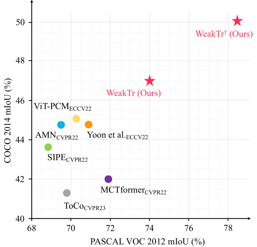
Figure 1: Weakly-supervised semantic segmentation performance on both PASCAL VOC 2012 $val$ and COCO 2014 $val$. The proposed WeakTr method obtains SOTA results and significantly outperforms previous WSSS methods. The $\dagger$ indicates the use of the improved ViT [39].

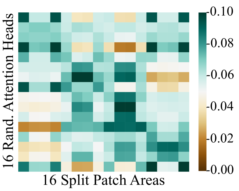
(a) Averaged attention values on different patches.

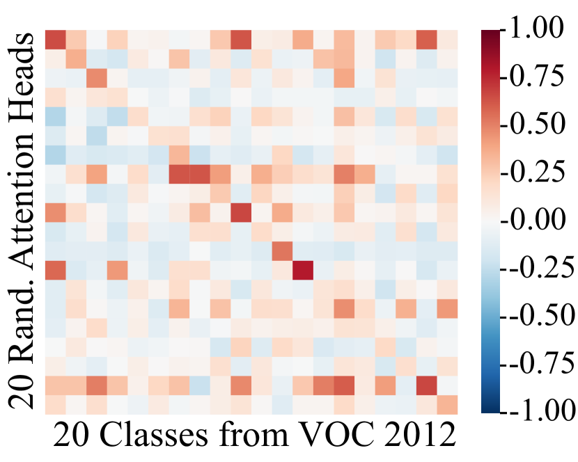
(b) PCC between averaged attention and class labels.

Figure 2: The statistical relationship between the attention values of different ViT heads and the patch position & the image category based on the whole VOC 2012 $train$ set. (a) shows the attention values, averaged over 20 classes, for 16 randomly selected heads on 4$\times$4 patches. (b) shows the Pearson correlation coefficients (PCC) between the attention values, averaged on spatial dimensions, for 20 randomly selected heads and the image classification labels.

With the success of vision transformers (ViT) [9], some methods [50, 12] propose to obtain CAM seeds with the assistance of transformer features and corresponding self-attention maps. The CAM generation phase usually contains 2 stages. Self-attention maps, representing relations between feature tokens, are adopted to enhance the coarse CAM in the post-processing stage. These methods directly average the attention maps across different heads and sum them by layers. However, as shown in Fig. 2, most different attention heads focus on different positions and object categories, which may contain information unrelated to the target object. Direct averaging and summing may lead to misleading information in the post-processing stage.

We propose an adaptive attention fusion module (AAF) to measure the importance of different attention heads for CAM, which is used for assigning weights for attention heads. To ensure that AAF can estimate accurate weights, we propose an end-to-end training strategy for CAM generation. During the training process, we apply the weights estimated by the AAF module to attention heads. The coarse CAM is thus optimized to be finer with the weighted self-attention maps. This module provides two terms of advantages from both CAM quality and optimization. For CAM quality, our improved CAM fits the foreground objects better than the mean-sum method and avoids misleading ones from irrelevant attention heads. For optimization, our end-to-end CAM generation method directly generates fine CAM and optimizes the AAF’s weight through classification loss during training.

As aforementioned, previous WSSS methods contain 3 phases: CAM generation, CAM refinement, and retraining, which are time-consuming and complex. We explore a more efficient way to perform retraining without refining the CAM seeds. Intuitively, regions with wrong labels in CAMs will affect the training of segmentation networks. Motivated by methods [13, 3, 31] for noisy label problems in classification networks, we propose a gradient clipping decoder for identifying confident regions. More specifically, image areas with a larger gradient are filtered out by a gradient clipping decoder. In this way, the segmentation network tends to be updated with smaller gradients for confident CAM regions. Our online retraining method enables the segmentation network to efficiently learn CAM regions that are biased towards correct labeling. Note that our online retraining network can not only be a high-performance segmentation network itself, but also be used as a labeling tool for producing high-quality pseudo labels for other segmentation networks.

The main contributions of this paper can be summarized as follows:

• We exploit the inherent properties of multi-layer, multi-head self-attention maps in plain ViT and devise an effective adaptive attention fusion strategy for generating high-quality class activation maps. This is the first work that sheds light on the importance of different attention heads for CAM and WSSS.

• We have explored a concise and efficient framework (WeakTr) based on plain ViT for WSSS. Our WeakTr framework enables end-to-end generation of high-quality CAMs and efficient online retraining through a simple but effective gradient clipping decoder. The overall training speed of the WeakTr framework is about 2.6 times that of the baseline framework.

• Our WeakTr fully explores the potential of plain ViT in the WSSS domain. State-of-the-art results are achieved on both challenging WSSS benchmarks, with 78.4% mIoU on PASCAL VOC 2012 [10] and 50.3% on COCO 2014 [28] validation sets respectively, significantly surpassing previous methods as shown in Fig. 1.

2 Related Work

2.1 Transformer in WSSS

The vision transformer has recently advanced the field of computer vision. ViT [9] transforms images into non-overlapping patch tokens, which are used as input along with a class token. The class token is then mapped to a class prediction using a fully connected layer. This model architecture without convolutional induction bias is considered to be promising. The TS-CAM [12] method uses the cross-attention map between the class token and patch tokens to obtain location cues in the weakly-supervised domain. The acquisition of the cross-attention map requires averaging the attention maps of different heads under the same layer and then summing over the different layers. After this, the cross-attention map is combined with the CAM obtained by processing the patch tokens using convolution. After this method, MCTformer [50] proposes multiple class tokens as input for learning the cross-attention maps of different classes. The CAM is additionally optimized by using the patch-attention maps in the post-processing stage. In addition, TransCAM [25] is based on the conformer [30] backbone, which is a mixture of transformer blocks and convolution. It also uses patch-attention maps to refine CAM at the CAM generation stage. However, most attention heads of the transformer notice different positions and classes in the image, which may contain information unrelated to the target object.

Unlike the above ViT-based methods, our WeakTr uses different weights to estimate the importance of the transformer’s attention heads. With an end-to-end strategy to optimize the adaptive attention fusion module, we could further improve the accuracy of the final attention result.

2.2 Image-level Supervised Learning

In order to obtain cues with only image-level labels, many methods focus on how to optimize CAM. The SEC method [18] spreads the sparse CAM labels by seed expansion. DSRG [16] combines the seed region growth method to expand CAM cues. A similar approach is DGCN [11], which assigns labels to regions around seeds by using traditional graph-cutting algorithms. AffinityNet [2] and IRNet [1] propagate the labels using the random walk method. AuxSegNet [49] propagates labels by learning the affinity of the cross-task. There are also methods that use adversarial erasing [15, 45] to help CAM focus more on the undiscriminating regions. SEAM [44] explores the consistency of CAM under different affine transformations. In addition, there are methods that choose to introduce web data, such as Co-segmentation [37] and STC [46].

However, using methods such as the AffinityNet [2] to refine the CAM and then using the refined pseudo mask to retrain the DeepLab [27, 6] network can be too complicated and time-consuming. Our proposed gradient clipping decoder enables the segmentation network to directly and efficiently learn from confident CAM areas without any CAM refinement.

3 Weakly-supervised Semantic Segmentation Transformer (WeakTr)

In this section, we first introduce the end-to-end CAM generation phase of the WeakTr framework, which comprises a plain ViT backbone and an adaptive attention fusion module for generating fine CAM end-to-end. We then discuss the online retraining phase of the WeakTr framework, which also employs the plain ViT backbone and a gradient clipping decoder.

3.1 End-to-End WeakTr CAM Generation

3.1.1 Plain ViT Backbone

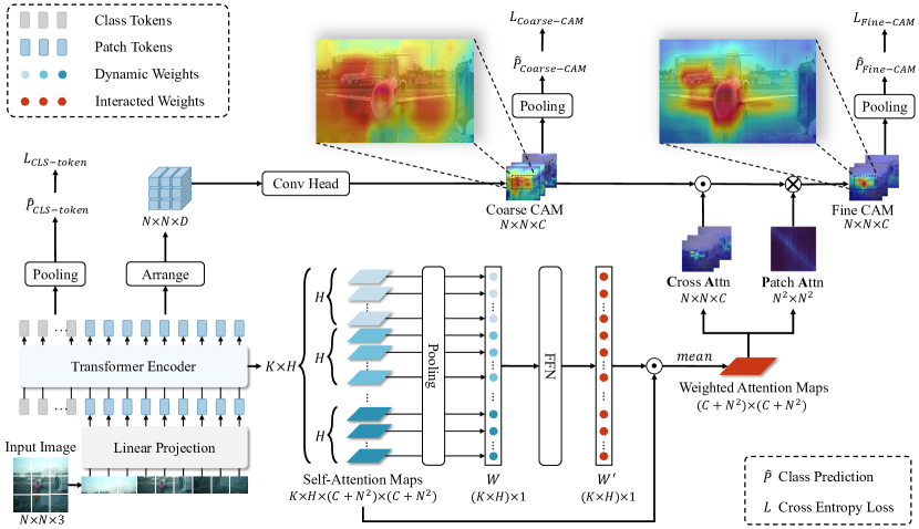
Figure 3: An overview of our proposed end-to-end WeakTr CAM generation. WeakTr first inputs the image patch tokens and multiple class tokens into the transformer encoder. Next, we generate coarse CAM by applying a convolution layer to the patch tokens. Then we use the adaptive attention fusion module to generate dynamic weights from all self-attention maps and make the dynamic weights interact via the feed-forward network (FFN). Finally, we optimize the coarse CAM into the fine CAM by using weighted cross-attention maps and weighted patch-attention maps. Class tokens, coarse CAM, and fine CAM finally generate predictions by pooling to compute the corresponding prediction loss.

As shown in Fig. 3, our framework uses the plain ViT as the backbone. First, we split an input image into $N^{2}$ patches, flatten them, and linearly map them into $N^{2}$ patch tokens. Furthermore, we generate $C$ learnable class tokens, where $C$ represents the total number of classification categories, and concatenate them with patch tokens as the transformer encoder’s input $T_{in}\in\mathbb{R}^{(C+N^{2})\times D}$, where $D$ is the dimension of input tokens.

The transformer encoder consists of $K$ encoding layers internally. Each layer consists of two sub-layers: a multi-head self-attention (MSA) and a multilayer perceptron (MLP). Layer Normalization (LN) is applied before every sub-layer, and residual connections after every sub-layer. In each encoding layer, we input tokens $T_{in}$ and receive $T_{out}$. The $T_{out}$ becomes the new $T_{in}$ for the next encoder layer, and so on for $K$ iterations.

3.1.2 Direct CAM Generation with Adaptive Attention Fusion

After going through the $K$ transformer layers, these tokens are then arranged as the final tokens $T_{final}\in\mathbb{R}^{(C+N^{2})\times D}$. In order to get a coarse CAM first, we need to extract the last $N^{2}$ patch tokens from $T_{final}$. Then we arrange the $N^{2}$ patch tokens, making them the $T_{final-patches}\in\mathbb{R}^{N\times N\times D}$. Next, we use a convolution layer to obtain the $CAM_{coarse}\in\mathbb{R}^{N\times N\times C}$ as follows:

$$T_{final-patches} =\mathrm{Arrange}(T_{final}[C+1:C+N^{2}])$$ (1)

$$CAM_{coarse} =\mathrm{Conv}(T_{final-patches}).$$ (2)

After obtaining the coarse CAM, we refine it using the self-attention maps of the transformer encoder. A single self-attention map has a shape of $(C+N^{2})^{2}$, allowing us to obtain the cross-attention maps of the $C$ class tokens for the $N^{2}$ patch tokens and the patch-attention maps of the $N^{2}$ patch tokens relative to themselves. The cross-attention maps have a shape of $N\times N\times C$, and the patch-attention maps have a shape of $N^{2}\times N^{2}$. Considering that the transformer encoder has $K$ encoding layers, each with $H$ attention heads, we can obtain the cross-attention maps as $CA\in\mathbb{R}^{(K\times H)\times N\times N\times C}$ and the patch-attention maps as $PA\in\mathbb{R}^{(K\times H)\times N^{2}\times N^{2}}$.

In order to combine the representation of all attention heads in all layers, previous WSSS methods [50, 25] have directly averaged the self-attention maps of different heads in the same layer, and then summed them by different layers. We find that this mean-sum approach to the deployment of transformer attention is rudimentary. As shown in Fig. 2, most different attention heads focus on different areas and classes. This indiscriminate approach to the attention heads tends to introduce more interference to the activation map of foreground objects. So we propose to utilize an adaptive attention fusion module to estimate the importance of different attention heads.

As shown in Fig. 3, first, we get the self-attention maps $A\in\mathbb{R}^{(K\times H)\times(C+N^{2})\times(C+N^{2})}$ corresponding to the attention heads of all transformer layers. Next, we get the corresponding dynamic weights $W\in\mathbb{R}^{(K\times H)\times 1}$ by applying pooling across the heads. Then we use an FFN network to interact with the information among the dynamic weights as follows:

$$W^{{}^{\prime}} =\mathrm{FFN}(\mathrm{Pooling}(A)),$$ (3)

where $\mathrm{Pooling}$ is the global average pooling and $W^{{}^{\prime}}\in\mathbb{R}^{(K\times H)\times 1}$ is the interacted weights for the attention heads . Finally, we multiply the interacted weights $W^{{}^{\prime}}$ back to the cross-attention maps $CA$ and the patch-attention maps $PA$ to get $\widehat{CA}$ and $\widehat{PA}$ respectively as follows:

$$\widehat{CA} =\frac{1}{KH}\sum_{i=1}^{K\cdot H}W^{{}^{\prime}}_{i}\cdot CA_{i}$$ (4)

$$\widehat{PA} =\frac{1}{KH}\sum_{i=1}^{K\cdot H}W^{{}^{\prime}}_{i}\cdot PA_{i},$$ (5)

where $\widehat{CA}\in\mathbb{R}^{N\times N\times C}$ and $\widehat{PA}\in\mathbb{R}^{N^{2}\times N^{2}}$ are the weighted results we get from self-attention maps by using the interacted weights $W^{{}^{\prime}}$. We have adopted the same method as MCTformer [50] and TransCAM [25] to combine $CAM_{coarse}$, $\widehat{CA}$, and $\widehat{PA}$.:

$$CAM_{fine} =\mathfrak{R}^{N\times N\times C}(\widehat{PA}\cdot\mathfrak{R}^{N^{2}\times C}(CAM_{coarse}\odot\widehat{CA})),$$ (6)

where $CAM_{fine}$ is the CAM guided by $\widehat{CA}$, and $\widehat{PA}$, $\mathfrak{R}^{N^{2}\times C}(\cdot)$ is the operator used to reshape the matrix to $N^{2}\times C$, $\mathfrak{R}^{N\times N\times C}(\cdot)$ is the operator used to reshape the matrix to $N\times N\times C$, and $\odot$ denotes the Hadamard product. As shown in Tab. 4 and the visualizations in the supplement, the weighted self-attention maps provide more accurate guidance for CAMs compared to the mean-sum self-attention maps.

3.1.3 End-to-End Fine CAM Training

The key to the adaptive attention fusion module’s ability to provide accurate weights lies in our end-to-end training strategy. End-to-end generation of fine CAMs allows the adaptive attention fusion module to perform supervised learning through image-level supervision. The process of improving coarse CAMs using self-attention maps to generate fine CAMs and calculating the loss function $L_{Fine-CAM}$ is fully differentiable. Therefore, the loss $L_{Fine-CAM}$ for classification can provide weak supervision guidance for weight allocation of attention maps. Under this guidance, attention heads that match the object of interest in terms of both attended categories and attended regions are encouraged to have greater weights assigned to them, while those that do not match have smaller weights. We add the $L_{Fine-CAM}$ to the $L_{CLS-token}$ and the $L_{Coarse-CAM}$ in Fig. 3 to get the total loss $\mathcal{L}$ as follows:

$$\mathcal{L} =L_{Fine-CAM}+L_{CLS-token}+L_{Coarse-CAM}.$$ (7)

3.2 WeakTr Online Retraining with Gradient Clipping Decoder

Traditionally, the low quality of CAMs in WSSS frameworks requires CAM refinement [2] phase before they could be used for retraining. This process can be tedious and lengthy. Our proposed online retraining method involves ViT and a gradient clipping decoder. It can directly train a high-performance semantic segmentation model using CAMs, bypassing the need for CAM refinement.

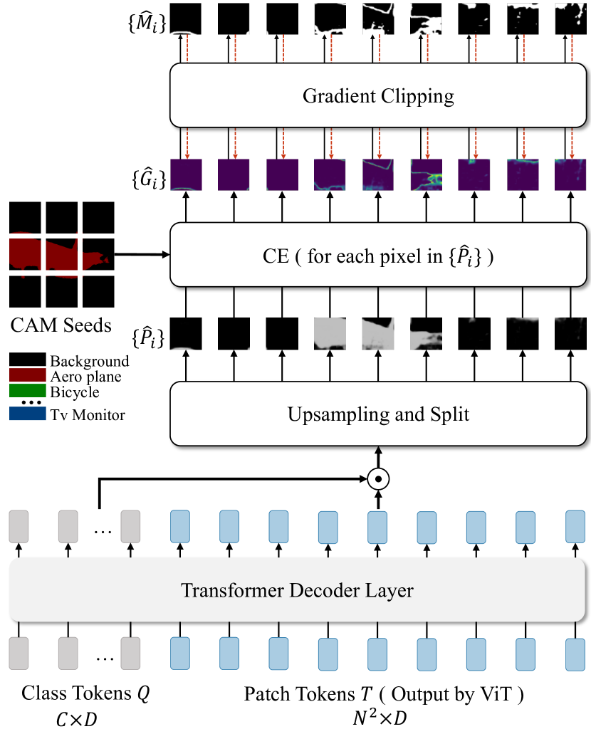
Figure 4: Architecture of our proposed gradient clipping decoder. The input of the gradient clipping decoder consists of two parts: class tokens $Q$ and patch tokens $T$ output by the ViT encoder. After the operation of the decoder layers, we first obtain the corresponding patch predictions by combining class tokens and patch tokens. Next, we upsample the obtained prediction and split the prediction into prediction patches $\{\hat{P}_{i}\}$. Then we calculate the gradient patches $\{\hat{G}_{i}\}$ with the CAM seeds. Finally, we dynamically generate the gradient clipping mask $\{\hat{M}_{i}\}$ and multiply the gradient clipping mask by the original gradient map. Please note that in this figure, we only show the structure of the gradient clipping decoder. During training, the ViT encoder and gradient clipping decoder are updated together.

As shown in Fig. 4, first we input the class tokens $Q\in\mathbb{R}^{C\times D}$ and the patch tokens $T\in\mathbb{R}^{N^{2}\times D}$ produced by the ViT encoder together into the transformer decoder layer to get the corresponding outputs $\hat{Q}\in\mathbb{R}^{C\times D}$ and $\hat{T}\in\mathbb{R}^{N^{2}\times D}$. Next, we use the L2-normalized $\hat{Q}_{norm}$ and $\hat{T}_{norm}$ to generate the corresponding predicted sequences. Then we pass the predicted sequences through LN and upsample them to get the prediction $\hat{P}\in\mathbb{R}^{O\times O\times C}$ as follows:

$$\hat{P} =\mathrm{Upsampling}(\mathrm{LN}(\frac{\hat{T}_{norm}\cdot\hat{Q}_{norm}^{\mathrm{T}}}{\sqrt{D}})),$$ (8)

where $(O,O)$ is the original resolution of the input image.

In noisy label problems, some works [13, 3, 31] have pointed out that samples with smaller gradients are more likely regarded as clean ones. In semantic segmentation tasks, we can treat each pixel as a sample and determine whether to clip the gradient at that pixel based on a threshold. The purpose of our gradient clipping decoder is to find a suitable threshold. To determine the gradient threshold, we considered two factors: the gradient across the entire image and the gradient within local regions. Firstly, we use the average gradient value of all pixels in the whole image as the global gradient constraint. Secondly, we divide pixels into patches to obtain local gradient constraints from patch regions, similar to ViT. The gradient clipping decoder fully considers these two constraints to judge if clips the gradient of each pixel. It clips regions with larger gradients, allowing the segmentation network to focus on learning regions with smaller gradients.

To compute the local gradient constraint, we split the prediction $\hat{P}\in\mathbb{R}^{O\times O\times C}$ into $L^{2}$ non-overlapping patches $\{\hat{P}_{i}\},i\in\{1,\dots,L^{2}\}$. The shape of each patch in $\{\hat{P}_{i}\}$ is $S\times S\times C$, and $L=O/S$. Please note that the patch size in $\{\hat{P}_{i}\}$ is unrelated to the image patch size in the ViT encoder. Using the CAM seeds generated from $CAM_{fine}$ and the prediction patches $\{\hat{P}_{i}\}$, we can calculate the gradient patches $\{\hat{G}_{i}\}$. Each gradient patch in $\{\hat{G}_{i}\}$ has a size of $S\times S$. Meanwhile, we can calculate the average gradient $\{\lambda_{i}\}$ for each gradient patch in $\{\hat{G}_{i}\}$ as follows:

$$\hat{G}_{i} =\mathrm{CE}(\hat{P}_{i},{CAMseeds}_{i}),i\in\{1,\dots,L^{2}\}$$ (9)

$$\lambda_{i} ={\mathrm{mean}(\hat{G}_{i})},i\in\{1,\dots,L^{2}\},$$ (10)

where $\mathrm{CE}$ is the cross-entropy loss calculated for each pixel. For each gradient patch in $\{\hat{G}_{i}\}$, we use $\{\lambda_{i}\}$ as a local constraint and the average of $\{\lambda_{i}\}$ as a global constraint $\lambda_{global}$.

$$\lambda_{global} =\frac{1}{L^{2}}\sum_{i=1}^{L^{2}}\lambda_{i}.$$ (11)

We choose the maximum of $\lambda_{global}$ and $\{\lambda_{i}\}$ as the threshold value for clipping mask $\{\hat{M}_{i}\}$ generation. In this way, the obtained $\{\hat{M}_{i}\}$ considers both local and global gradient constraints, achieving the discarding of patch regions with relatively large gradients.

$$\hat{M}_{i} =\left\{\begin{array}[]{ll}1,&\hat{G}_{i,(j,k)}\leq\max(\lambda_{i},\lambda_{global})\\ 0,&\hat{G}_{i,(j,k)}~{}\textgreater~{}\max(\lambda_{i},\lambda_{global})\end{array}\right.,$$ (14)

where $1\leq j\leq S$, $1\leq k\leq S$ and $\mathrm{max}$ is the maximum operation.

However, the selection of confident CAM regions by the gradient clipping decoder is not reliable enough at the beginning of the segmentation network training. So we set the clipping start value $\tau$ to determine whether to clip. Only when the global mean gradient $\lambda_{global}$ of the current batch is lower than $\tau$, we clip the gradient as follows:

$$\hat{G}^{{}^{\prime}}_{i} =\left\{\begin{array}[]{ll}\hat{G}_{i}\odot\hat{M}_{i},&\lambda_{global}\leq\tau\\ \hat{G}_{i},&\lambda_{global}~{}\textgreater~{}\tau\end{array}\right..$$ (17)

Finally, we get the masked gradient patches $\{\hat{G}^{{}^{\prime}}_{i}\}$ and back-propagate their average value. By doing so, We dynamically select regions with smaller gradients as confident CAM regions to prioritize learning for the segmentation network. During inference, we apply the Conditional Random Field (CRF) [19] to improve the segmentation quality.

4 Experiments

4.1 Experimental Setup

Datasets

We evaluate our WeakTr on the PASCAL VOC 2012 [10] dataset and the COCO 2014 [28] dataset. The PASCAL VOC 2012 dataset has 20 foreground categories and 1 background category. This dataset has three separate splits: the training set (includes 1464 images), the validation set (includes 1449 images), and the test set (includes 1456 images). In addition, WSSS methods usually use SBD [14] annotations to increase the training set to 10582 images. For another COCO14 dataset, which has 80 object categories for segmentation. The validation set has 40137 images, and the training set has 82081 images. We use mean intersection over union (mIoU) to evaluate the validation set in our experiments.

Implementation Details

For the WeakTr’s CAM generation, we adopt DeiT-S [43] as the backbone, and we train all the models using the AdamW [29] optimizer. We take Segmenter [40] as our retraining baseline. For WeakTr’s online retraining, we replace the Segmenter’s decoder with our gradient clipping decoder. Following Segmenter’s manner, our online retraining uses the improved ViT [39], which is pre-trained on ImageNet-21k [8] and fine-tuned on ImageNet-1k [36] at a resolution of 384. To give a fair comparison, we also evaluate our gradient clipping decoder with DeiT-S, which is pre-trained on ImageNet-1k.

4.2 Comparisons with State-of-the-art Methods

PASCAL VOC 2012

At first, we give the quantitative results of CAM and mask for VOC 2012 in Tab. 1. In the second column, it can be observed that the fine CAM of WeakTr achieves 4.5% and 2.6% higher results compared to MCTformer [50] and ViT-PCM [33], respectively. The third column shows the quality of the pseudo mask obtained by the CAM refinement. It can be seen that our result is 6.0% higher than CLIMS [48].

Table 1: Evaluation of the CAM and the corresponding pseudo segmentation ground-truth mask (Mask) in terms of mIoU (%) on the PASCAL VOC 2012 $train$ set. We mark the best results in bold.

Method	CAM	Mask
BES$\ {}_{\mathrm{ECCV20}}$ [5]	49.6	67.2
SC-CAM$\ {}_{\mathrm{CVPR20}}$ [4]	50.9	63.4
SEAM$\ {}_{\mathrm{CVPR20}}$ [44]	55.4	63.6
CONTA$\ {}_{\mathrm{NeurIPS20}}$ [52]	56.2	67.9
AdvCAM$\ {}_{\mathrm{CVPR21}}$ [21]	55.6	69.9
ECS-Net$\ {}_{\mathrm{ICCV21}}$ [42]	56.6	67.8
OC-CSE$\ {}_{\mathrm{ICCV21}}$ [20]	56.0	66.9
VWE$\ {}_{\mathrm{IJCV22}}$ [34]	57.3	71.4
CLIMS$\ {}_{\mathrm{CVPR22}}$ [48]	56.6	70.5
MCTformer$\ {}_{\mathrm{CVPR22}}$ [50]	61.7	69.1
ViT-PCM$\ {}_{\mathrm{ECCV22}}$ [33]	63.6	67.1
Yoon et al.$\ {}_{\mathrm{ECCV22}}$ [51]	56.0	71.0
WeakTr w/ DeiT-S (Ours)	66.2	76.5

Table 2: Evaluation of the final segmentation results in terms of mIoU (%) on the PASCAL VOC 2012 $val$ and $test$ sets. The $Sup.$ column denotes the type of supervision used for training including full supervision ($\mathcal{F}$), image-level labels ($\mathcal{I}$), saliency maps ($\mathcal{S}$), and bounding box labels ($\mathcal{B}$). The $\dagger$ indicates the use of the improved ViT pre-trained model. We mark the best WSSS results in bold.

Method	Backbone	$Sup.$	$val$	$test$
Segmenter$\ {}_{\mathrm{ICCV21}}$ [40]	DeiT-S	$\mathcal{F}$	79.7	79.6
Segmenter† $\ {}_{\mathrm{ICCV21}}$ [40]	ViT-S		82.6	83.1
DeepLabV2$\ {}_{\mathrm{TPAMI17}}$ [6]	ResNet101		77.7	79.7
WideResNet38$\ {}_{\mathrm{PR19}}$ [47]	ResNet38		80.8	82.5
BCM$\ {}_{\mathrm{CVPR19}}$ [38]	ResNet101	$\mathcal{I}+\mathcal{B}$	70.2	-
BBAM$\ {}_{\mathrm{CVPR21}}$ [23]	ResNet101		73.7	73.7
EPS$\ {}_{\mathrm{CVPR21}}$ [24]	ResNet101	$\mathcal{I}+\mathcal{S}$	71.0	71.8
L2G$\ {}_{\mathrm{CVPR22}}$ [17]	ResNet101		72.1	71.7
SEAM$\ {}_{\mathrm{CVPR20}}$ [44]	ResNet38	$\mathcal{I}$	64.5	65.7
AdvCAM$\ {}_{\mathrm{CVPR21}}$ [21]	ResNet101		68.1	68.0
OC-CSE$\ {}_{\mathrm{ICCV21}}$ [20]	ResNet38		68.4	68.2
CPN$\ {}_{\mathrm{ICCV21}}$ [53]	ResNet38		67.8	68.5
VWE$\ {}_{\mathrm{IJCV22}}$ [34]	ResNet101		70.6	70.7
CLIMS$\ {}_{\mathrm{CVPR22}}$ [48]	ResNet101		70.4	70.0
MCTformer$\ {}_{\mathrm{CVPR22}}$ [50]	ResNet38		71.9	71.6
SIPE$\ {}_{\mathrm{CVPR22}}$ [7]	ResNet101		68.8	69.7
W-OoD$\ {}_{\mathrm{CVPR22}}$ [22]	ResNet38		70.7	70.1
AMN$\ {}_{\mathrm{CVPR22}}$ [22]	ResNet101		69.5	69.6
ViT-PCM$\ {}_{\mathrm{ECCV22}}$ [33]	ResNet101		70.3	70.9
Yoon et al.$\ {}_{\mathrm{ECCV22}}$ [51]	ResNet38		70.9	71.7
ToCo$\ {}_{\mathrm{CVPR23}}$ [35]	ViT-B		69.8	70.5
WeakTr (Ours)	DeiT-S	$\mathcal{I}$	74.0	74.1
WeakTr† (Ours)	ViT-S		78.4	79.0

Then, we give the quantitative results of the final segmentation results on the VOC 2012 in Tab. 2. Our WeakTr method results are obtained via online retraining using the CRF-processed CAM, and we show the online retraining results using DeiT-S [43] and improved ViT-S [39], respectively. Our approach outperforms previous techniques on both the $val$ and $test$ sets.

We also list the fully-supervised methods Segmenter-DeiT-S [40] and Segmenter-ViT-S [40] as upper bounds for our WeakTr. We use $\delta$ to express the performance gap between the weakly-supervised method and the upper bound. The $\delta$ of WeakTr-DeiT-S compared to the upper bound method is -5.7% and -5.5% for the $val$ and $train$ sets, respectively. The $\delta$ of WeakTr-ViT-S compared to the upper bound method is -4.2% and -4.1% for $val$ and $train$ sets, respectively. Our baseline method, MCTformer, has a $\delta$ of -8.9% and -10.9% compared to its upper bound method, WideResNet38 [47], for $val$ and $train$ sets, respectively. In summary, our WeakTr approach proves to be better than other methods at reducing the performance gap between weakly-supervised and fully-supervised methods.

COCO 2014

We give the quantitative results of the final segmentation results on COCO 2014 in Tab. 3. Our WeakTr results are all being obtained through online retraining with the CRF-processed CAM, and our WeakTr-ViT-S can achieve 8.3% higher results on the $val$ set compared to MCTformer [50].

Table 3: Evaluation of the final segmentation results in terms of mIoU (%) on the COCO 2014 $val$ set. We mark the best WSSS result in bold.

Method	Backbone	$Sup.$	$val$
EPS$\ {}_{\mathrm{CVPR21}}$ [24]	ResNet101	$\mathcal{I}+\mathcal{S}$	35.7
AuxSegNet$\ {}_{\mathrm{ICCV21}}$ [49]	ResNet38		33.9
SEAM$\ {}_{\mathrm{CVPR20}}$ [44]	ResNet38	$\mathcal{I}$	31.9
OC-CSE$\ {}_{\mathrm{ICCV21}}$ [20]	ResNet38		36.4
CDA$\ {}_{\mathrm{ICCV21}}$ [41]	ResNet38		33.2
VWE$\ {}_{\mathrm{IJCV22}}$ [34]	ResNet101		36.2
URN$\ {}_{\mathrm{AAAI22}}$ [26]	Res2Net101		41.5
MCTformer$\ {}_{\mathrm{CVPR22}}$ [50]	ResNet38		42.0
SIPE$\ {}_{\mathrm{CVPR22}}$ [7]	ResNet38		43.6
AMN$\ {}_{\mathrm{CVPR22}}$ [7]	ResNet101		44.7
ViT-PCM$\ {}_{\mathrm{ECCV22}}$ [33]	ResNet101		45.0
Yoon et al.$\ {}_{\mathrm{ECCV22}}$ [51]	ResNet38		44.8
ToCo$\ {}_{\mathrm{CVPR23}}$ [35]	ViT-B		41.3
WeakTr (Ours)	DeiT-S	$\mathcal{I}$	46.9
WeakTr† (Ours)	ViT-S	$\mathcal{I}$	50.3

Table 4: Ablation study for the adaptive attention fusion module in terms of precision (%), recall (%) and mIoU (%) on the PASCAL VOC 2012 $train$ set. “mean-sum” means the attention maps of ViT are aggregated using mean-sum. “w/ rand. fixed $W$” means the use of randomly initialized fixed weights $W$ instead of the dynamic weights $W$ in the adaptive attention fusion module. “w/ CRF” means the adoption of CRF for processing. We mark the best results in bold.

Method (CAM generation)	Precision	Recall	mIoU
Baseline (mean-sum)	75.0	77.9	61.7
WeakTr (w/ rand. fixed $W$)	75.6	82.4	65.3
WeakTr	76.4	83.1	66.2
WeakTr (w/ CRF)	78.9	83.7	68.7

4.3 Ablation Studies

Improvements of Adaptive Attention Fusion

To further analyze the improvements brought by our proposed adaptive attention fusion, we give the quantitative results of CAM on the VOC 2012 $train$ set in Tab. 4. Here, we use MCTformer as the baseline, which aggregates the self-attention maps using mean-sum. The adaptive attention fusion module first obtains dynamic weights $W$ from the self-attention maps and then passes $W$ through FFN to obtain the final weights $W^{\prime}$. When we try to use randomly initialized fixed $W$ instead of dynamic weights $W$, the experiment shows that even without the dynamic prior of $W$, FFN can still help WeakTr fit the weights for self-attention maps (3.6% higher than the baseline). With the prior brought by dynamic weights $W$, WeakTr can fit better weights for self-attention maps.

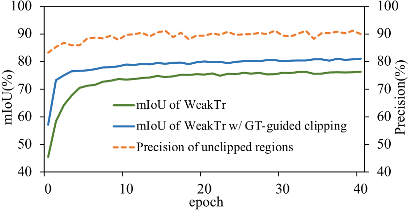
Figure 5: The effectiveness of the gradient clipping decoder and the upper bound for online retraining. ‘orange curve’: the precision of the pseudo labels for unclipped regions in the gradient clipping decoder. ‘green curve’: the mIoU of the WeakTr’s online retraining. ‘blue curve’: the mIoU of the WeakTr’s online retraining with GT-guided clipping, representing the upper bound of online retraining.

Improvements of gradient clipping decoder

To further analyze the improvements brought by our proposed gradient clipping decoder, we conduct ablation experiments for the gradient clipping decoder and present the results in Tab. 5. Here, we take the naive decoder as our baseline. When using a gradient clipping decoder with a start value of 1.2, we could get 1.5% higher mIoU than the baseline. We obtain a 2.5% higher mIoU than the baseline after processing the results with CRF in the gradient clipping decoder. These experiments demonstrate that our proposed gradient clipping decoder is more suitable for the WSSS task than the naive decoder.

We also conduct an ablation study for the gradient patches shape, as shown in Tab. 6, a gradient patch with a resolution of (120, 120) can improve the performance of the gradient clipping decoder by allowing it to better utilize the gradient threshold constraint.

We further investigated the effectiveness of the gradient clipping decoder during the training process. As shown in Fig. 5, the results show that the precision of the regions retained by the gradient clipping decoder is around 90%, compared to only 78.9% for CAMs in Tab. 4. Although the gradient clipping decoder discards some gradient regions, it ensures that the learned regions are mostly accurate. The blue curve also shows the upper bound that online retraining can reach when guided by ground truth for gradient clipping.

Improvements of framework training time

To further analyze the improvements in training time brought by our WeakTr framework, we conduct experiments to display training time in Tab. 11(b). On one hand, WeakTr introduces the AAF module for end-to-end training, so the CAM generation phase takes 20 minutes longer than MCTformer. On the other hand, WeakTr’s online retraining saves more than 2/3 of the time compared to MCTformer’s CAM refinement and retraining. Overall, the WeakTr framework takes more than 60% less time than MCTformer and has a total speed improvement of 2.6 times.

Table 5: Ablation study for the start value $\tau$ of the gradient clipping decoder in terms of mIoU (%) on the PASCAL VOC 2012 $val$ set. We mark the best result in bold.

Naive Decoder (Baseline)	Gradient Clipping Decoder						$val$
7
	start value $\tau$					CRF
6
	1.6	1.4	1.2	1.0	0.8
$\checkmark$							71.5
			$\checkmark$				73.0
			$\checkmark$			$\checkmark$	74.0
	$\checkmark$					$\checkmark$	73.6
		$\checkmark$				$\checkmark$	73.7
				$\checkmark$		$\checkmark$	73.5
					$\checkmark$	$\checkmark$	73.4

Table 6: Ablation study for the gradient patches shape $S$ of the gradient clipping decoder in terms of mIoU (%) on the PASCAL VOC 2012 $val$ set. We mark the best result in bold.

$S$	480	240	160	120	96
$val$	73.3	73.3	73.5	74.0	73.3

Table 7: Training time comparisons. We report the detailed training time for MCTformer and our WeakTr. All the experiments were launched using 1 TITAN X GPU.

(a) Training time of MCTformer framework. MCTformer consists of 3 phases and takes a total of 30.3 hours.

Method	CAM	CAM	Retraining
	Generation	Refinement
MCTformer	2 hrs 20 mins	12 hrs	16 hrs

(b) Training time of WeakTr framework. WeakTr consists of 2 phases and takes a total of 11.6 hours.

Method	CAM Generation	Online Retraining
WeakTr (Ours)	2 hrs 40 mins	9 hrs

5 Conclusion

We propose WeakTr for fully exploring the capacity of plain ViT in the field of weakly-supervised semantic segmentation, achieving state-of-the-art results of WSSS. The key insights of WeakTr are directly generating high-quality CAMs in ViT by adaptive multi-layer multi-head attention fusion and online retraining confident CAM regions with lower gradients through gradient clipping. We hope our work can motivate more studies to understand ViT and propose ViT-based methods to narrow the gap between fully-supervised and weakly-supervised semantic segmentation methods.

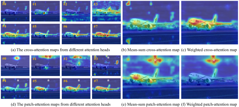
Figure 6: Comparison of the mean-sum results and the weight-based results. (a) shows the cross-attention maps from the different attention heads for the “plane” category. (b) shows the result obtained by the original mean-sum approach. (c) shows the result obtained by our proposed weight-based approach. (d) shows the patch-attention maps from the different attention heads corresponding to the “background” point. (We denote the query point with the “$\star$”) (e) shows the result obtained by the original mean-sum approach. (f) shows the result obtained by our proposed weight-based approach.

Appendix A Appendix

A.1 Implementation Details

WeakTr CAM Generation

During CAM generation, we use the DeiT-S/16 pretrained on ImageNet as the backbone. The adaptive attention fusion module consists of the global average pooling layer and a 2-layer feed-forward network (FFN) with hidden dimension 18, followed by a sigmoid activation function. During our training process, we use the AdamW [29] optimizer with a batch size of 64 and a weight decay of 0.05. The learning rate is linearly ramped up during the first 5 epochs to its base value determined with the following linear scaling rule: $lr=0.0004\times\mathrm{batchsize}/512$. After the warm-up, we decay the learning rate with a cosine schedule. In our model shown in Fig. 3, we compute three classification losses: $L_{CLS-token}$, $L_{Coarse-CAM}$, and $L_{Fine-CAM}$. For all three losses, we choose to use the multi-label soft margin loss computed between the image-level ground-truth labels $y$ and the class predictions $\hat{y}$ as follows:

$$Loss(\hat{y},y)=-\frac{1}{C}\sum_{i}^{C}y_{i}*log(\frac{1}{1+exp(-\hat{y_{i}})})$$ (18)

$$+(1-y_{i})*log(\frac{exp(-\hat{y_{i}})}{1+exp(-\hat{y_{i}})})$$ (19)

where $C$ is the number of classification categories.

At test time, we use the multi-scale strategy and the CRF [19] for post-processing.

WeakTr Online Retraining

At the retraining time, we use the stochastic gradient descent (SGD) [32] optimizer with a batch size of 4, a momentum parameter of 0.9, and a weight decay of 0. The learning rate is set to 0.0001 and decayed using a polynomial scheduler. Besides, we set the hierarchical learning rate for the transformer encoder to be 0.1 times the total learning rate. For the hyperparameters of the gradient clipping decoder, we choose the shape $S$ of 120 for the gradient patches and the start value $\tau$ of 1.2. At test time, we also use the multi-scale strategy and the CRF for post-processing.

A.2 Additional Ablations

Visual Comparison of Attention Maps

In Fig. 6, we show the visualization of the cross-attention maps and patch-attention maps. Firstly, as shown in Fig. 6 (a-c), we make a comparison between the fused cross-attention map of the “plane” category obtained by the mean-sum method and our weighted method, respectively. It demonstrates that the mean-sum method is more susceptible to being misled by the incorrect cross-attention maps from different attention heads, as shown in Fig. 6 (a). In contrast, our weighted method performs better by avoiding being misled by false information.

Besides, as shown in Fig. 6 (d-f), we also make a comparison between the fused patch-attention map obtained by the two aforementioned methods. Specially, we select to display the patch-attention corresponding to the “background” query point (denoted with a “$\star$”) and should focus on the “background” areas. However, as shown in Fig. 6 (d), there are some patch-attention maps that establish a class activation response with the foreground areas. This causes the mean-sum patch-attention map to be misled and creates a connection between the “background” and “plane” category areas in the final results as shown in Fig. 6 (e). As shown in Fig. 6 (f), our weighted method solved the problem mentioned above correctly.

Impact of Components in the AAF

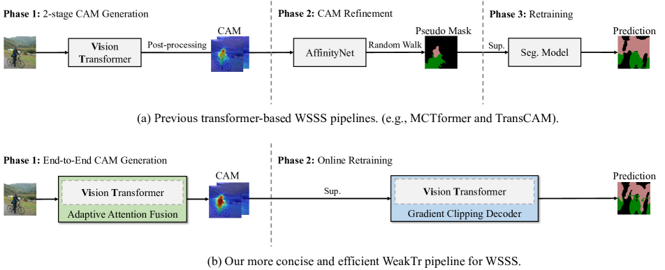
Figure 7: Comparison of the previous transformer-based WSSS frameworks and our WeakTr framework. Our proposed WeakTr framework is more concise and efficient compared to the previous transformer-based WSSS frameworks. We replace the 2-stage CAM generation with an end-to-end CAM generation using the adaptive attention fusion module, which greatly optimizes the guidance of the transformer attention for the CAM localization. Additionally, we introduce an online retraining method that directly uses CAM for supervised training, eliminating the need for cumbersome CAM refinement and retraining phases. Our gradient clipping decoder enables the network to prioritize learning confident pseudo label regions. The segmentation network of the online retraining method can serve as a segmentation model for inference on the $val$ and $test$ sets and also replace the previous AffinityNet to generate high-quality pseudo masks.

We use the adaptive attention fusion module to measure the importance of different attention heads, which consists of a pooling layer, an FFN, and a sigmoid activation function. We conduct ablation studies for the pooling layer and FFN to determine the impact of each component in the adaptive attention fusion module.

As shown in Tab. 8, increasing the hidden dimension of the FFN does not lead to greater improvement. This indicates that we only need a lightweight FFN network to fuse the information from the different attention heads. Through this fusing operation, we can obtain relatively accurate attention weights.

Table 8: Ablation study for the hidden dimension of FFN in the adaptive attention fusion module in terms of mIoU (%) on the PASCAL VOC 2012 $train$ set. We mark the best result in bold.

hidden dimension	144	72	36	18	9
$train$	65.6	66.0	65.4	66.2	65.8

As shown in Tab. 9, the results obtained using the max pooling and the average pooling are the same. In fact, the difference between the results of them is less than 0.003% mIoU. The results indicate that our adaptive attention fusion module performs robustly for both max pooling and average pooling. We can obtain accurate feature representations of various attention heads using different pooling methods and effectively interact with them using subsequent FFN.

Table 9: Ablation study for the different pooling layer in the adaptive attention fusion module in terms of mIoU (%) on the PASCAL VOC 2012 $train$ set.

	max pooling	average pooling
$train$	66.2	66.2

Table 10: Complexity of models. AffinityNet is used to refine the CAM for the previous method. WideResNet38 is used to retrain the pseudo masks for the previous method. WeakTr is our online retraining method with the DeiT-S backbone.

Model	Image size	#Params (M)	MACs (G)
AffinityNet[2]	480$\times$480	105.3	460.2
WideResNet38[47]	480$\times$480	124.2	600.0
WeakTr (Ours)	480$\times$480	26.3	23.0

Model Complexity of WeakTr Online Retraining

As shown in Fig. 7 (a), after generating the CAM, previous methods typically used the AffinityNet [2] to refine the CAM and then used the segmentation networks for retraining, e.g., WideResNet38 [47]. Our proposed online retraining with a gradient clipping decoder, which replaces the refinement and the retraining phases, fully explores the potential of plain ViT. As shown in Tab. 1 and Tab. 2, in terms of quantitative results, WeakTr’s online retraining can perform better than the combination of the AffinityNet and the WideResNet38. At the same input size, we compare the number of parameters and the multiply-add calculations (MACs) for WeakTr’s online retraining network, AffinityNet, and WideResNet38.

As shown in Tab. 10, our online retraining method has significantly less complexity and parameters than both AffinityNet and WideResNet38. It demonstrates that our online retraining effectively makes use of the plain ViT with a gradient clipping decoder.

Detailed Framework Training Time Comparison

In Tab. 11(b), we show the framework training time comparison between MCTformer [50] and WeakTr. To give a more detailed explanation, we display the sub-process training time of each phase in Tab. 11(b). Firstly, we show the MCTformer framework training time in Tab. 11(b) (a). The CAM generation phase consists of network training and post-processing to generate CAM. The CAM refinement phase consists of the affinity label generation from the CAM, AffinityNet [2] training, and the random walk to refine the CAM. The retraining phase only has a training process. For the comparison, we give the WeakTr framework training time in Tab. 11(b) (b). The CAM generation phase has the aforementioned two processes, which need a little more time because of the AAF module. The online retraining, which replaces the CAM refinement and retraining phases, only has a training process that takes 9 hours, which is 18.8 hours less than the 27.8 hours MCTformer requires for the two phases.

Table 11: Training time comparisons. We report the more detailed training time for MCTformer and our WeakTr. All the experiments were launched using 1 NVIDIA TITAN X GPU.

(a) Training time of MCTformer framework. MCTformer consists of 3 phases and takes a total of 30.3 hours.

Method	CAM Generation		CAM Refinement			Retraining
6
MCTformer	Training	Post-processing	Affinity Label Generation	AffinityNet Training	Random Walk	Training
7
	1 hrs 13 mins	1 hrs 10 mins	3 hrs	8 hrs	40 mins	16 hrs

(b) Training time of WeakTr framework. WeakTr consists of 2 phases and takes a total of 11.6 hours.

Method	CAM Generation		Online Retraining
3
WeakTr	Training	Post-processing	Training
4
	1 hrs 23 mins	1 hrs 20 mins	9 hrs

A.3 Additional Quantitative Results

Gaps between WSSS Methods and Upper Bounds

As shown in Tab. 12, we show the final semantic segmentation results on the PASCAL VOC 2012 $val$ and $test$ sets, as well as the gap $\delta$ between the weakly-supervised method and the upper bound. Among the weakly-supervised semantic segmentation methods based on image-level supervision, our WeakTr achieves a $\delta$ of -5.7% and -5.5% for the $val$ and $test$ sets, respectively. For the methods using DeeplabV2 [6] pre-trained on COCO as the upper bound, VWE [34] obtained the minimum $\delta$ of -7.1% for the $val$ set and the minimum $\delta$ of -9.0% for the $test$ set. For the methods using WideResNet38 [47] as the upper bound, MCTformer [50] obtained the minimum $\delta$ of -8.9% for the $val$ set and Yoon et al. [51] obtained the minimum $\delta$ of -10.8% for the $test$ set. Furthermore, our WeakTr^† achieves the minimum $\delta$ of -4.2% and -4.1% for the $val$ and $test$ sets with the upper bound Segmenter^† [40] as the upper bound.

These results demonstrate that our proposed online retraining with a gradient clipping decoder takes advantage of the contextual patch tokens output by plain ViT and effectively accomplishes self-correction. Our plain ViT-based online retraining significantly bridges the gap between weakly-supervised and fully-supervised methods, which proves the potential of plain ViT in the WSSS field.

Table 12: Evaluation of the final segmentation results in terms of mIoU (%) on the PASCAL VOC 2012 $val$ and $test$ sets. The upper bound methods with fully-supervised are denoted by a gray background. The $\dagger$ indicates using the improved ViT pre-trained model. The red numbers denote the performance gaps between the weakly-supervised methods and the upper bounds. We mark the best WSSS results in bold.

Method	Backbone	$val$	$test$
DeeplabV2$\ {}_{\mathrm{TPAMI17}}$ [6]	ResNet101	77.7	79.7
SC-CAM$\ {}_{\mathrm{CVPR20}}$ [4]	ResNet101	66.1-11.6	65.9-13.8
VWE$\ {}_{\mathrm{IJCV22}}$ [34]	ResNet101	70.6-7.1	70.7-9.0
CLIMS$\ {}_{\mathrm{CVPR22}}$ [48]	ResNet101	70.4-7.3	70.0-9.7
WideResNet38$\ {}_{\mathrm{PR19}}$ [47]	ResNet38	80.8	82.5
SEAM$\ {}_{\mathrm{CVPR20}}$ [44]	ResNet38	64.5-16.3	65.7-16.8
OC-CSE$\ {}_{\mathrm{ICCV21}}$ [20]	ResNet38	68.4-12.4	68.2-14.3
CPN$\ {}_{\mathrm{ICCV21}}$ [53]	ResNet38	67.8-13.0	68.5-14.0
MCTformer$\ {}_{\mathrm{CVPR22}}$ [50]	ResNet38	71.9-8.9	71.6-10.9
SIPE$\ {}_{\mathrm{CVPR22}}$ [7]	ResNet38	68.2-12.6	69.5-13.0
W-OoD$\ {}_{\mathrm{CVPR22}}$ [22]	ResNet38	70.7-10.1	70.1-12.4
Yoon et al.$\ {}_{\mathrm{ECCV22}}$ [51]	ResNet38	70.9-9.9	71.7-10.8
Segmenter$\ {}_{\mathrm{ICCV21}}$ [40]	DeiT-S	79.7	79.6
WeakTr (Ours)	DeiT-S	74.0-5.7	74.1-5.5
Segmenter†$\ {}_{\mathrm{ICCV21}}$ [40]	ViT-S	82.6	83.1
WeakTr† (Ours)	ViT-S	78.4-4.2	79.0-4.1

PASCAL VOC 2012 Per-class Results

Table 13: Comparison of per-class segmentation results in terms of IoUs on the PASCAL VOC 2012 $val$ set The ^† indicates online retraining using the improved ViT pre-trained model. We mark the best results in bold.

Method	bkg	plane	bike	bird	boat	bottle	bus	car	cat	chair	cow
AdvCAM CVPR21[21]	90.0	79.8	34.1	82.6	63.3	70.5	89.4	76.0	87.3	31.4	81.3
CPN ICCV21[53]	89.9	75.1	32.9	87.8	60.9	69.5	87.7	79.5	89.0	28.0	80.9
OC-CSE ICCV21[20]	90.2	82.9	35.1	86.8	59.4	70.6	82.5	78.1	87.4	30.1	79.4
MCTformer CVPR22[50]	91.9	78.3	39.5	89.9	55.9	76.7	81.8	79.0	90.7	32.6	87.1
WeakTr (Ours)	92.4	88.6	44.4	89.9	71.0	80.8	88.9	80.4	93.1	35.5	85.2
WeakTr† (Ours)	93.7	90.0	49.9	93.1	76.5	81.8	90.6	86.6	93.6	45.7	93.7
Method	table	dog	horse	mbk	person	plant	sheep	sofa	train	tv	mIoU
AdvCAM CVPR21[21]	33.1	82.5	80.8	74.0	72.9	50.3	82.3	42.2	74.1	52.9	68.1
CPN ICCV21[53]	34.8	83.4	79.7	74.7	66.9	56.5	82.7	44.9	73.1	45.7	67.8
OC-CSE ICCV21[20]	45.9	83.1	83.4	75.7	73.4	48.1	89.3	42.7	60.4	52.3	68.4
MCTformer CVPR22[50]	57.2	87.0	84.6	77.4	79.2	55.1	89.2	47.2	70.4	58.8	71.9
WeakTr (Ours)	50.8	85.5	84.4	78.4	76.9	60.0	90.2	44.0	76.6	56.2	74.0
WeakTr† (Ours)	57.7	90.5	90.9	81.5	80.9	59.6	93.2	58.0	78.1	59.6	78.4

Table 14: Comparison of per-class segmentation results in terms of IoUs on the PASCAL VOC 2012 $test$ set. The ^† indicates online retraining using the improved ViT pre-trained model. We mark the best results in bold.

Method	bkg	plane	bike	bird	boat	bottle	bus	car	cat	chair	cow
AdvCAM CVPR21[21]	90.1	81.2	33.6	80.4	52.4	66.6	87.1	80.5	87.2	28.9	80.1
CPN ICCV21[53]	90.4	79.8	32.9	85.8	52.9	66.4	87.2	81.4	87.6	28.2	79.7
MCTformer CVPR22[50]	90.9	76.0	37.2	79.1	54.1	69.0	78.1	78.0	86.1	30.3	79.5
WeakTr (Ours)	92.7	90.4	45.9	81.6	71.2	72.8	90.5	82.7	92.6	31.9	77.9
WeakTr† (Ours)	94.0	89.3	49.3	89.7	72.9	78.3	87.9	88.7	95.8	40.0	91.5
Method	table	dog	horse	mbk	person	plant	sheep	sofa	train	tv	mIoU
AdvCAM CVPR21[21]	38.5	84.0	83.0	79.5	71.9	47.5	80.8	59.1	65.4	49.7	68.0
CPN ICCV21[53]	50.2	82.9	80.4	78.9	70.6	51.2	83.4	55.4	68.5	44.6	68.5
MCTformer CVPR22[50]	58.3	81.7	81.1	77.0	76.4	49.2	80.0	55.1	65.4	54.5	68.4
WeakTr (Ours)	58.2	89.4	80.6	81.2	78.2	70.1	86.1	60.0	70.0	52.8	74.1
WeakTr† (Ours)	66.3	91.7	91.8	89.2	80.7	72.7	92.1	69.3	70.1	57.2	79.0

Table 15: Comparison of per-class segmentation results in terms of IoUs on the COCO 2014 $val$ set. We mark the best results in bold.

Class	MCTformer $\mathrm{CVPR22}$[50]	WeakTr (Ours)	WeakTr† (Ours)	Class	MCTformer $\mathrm{CVPR22}$[50]	WeakTr (Ours)	WeakTr† (Ours)
background	82.4	82.9	84.3	wine glass	27.0	28.4	36.1
person	62.6	65.0	67.8	cup	29.0	27.8	42.2
bicycle	47.4	51.4	53.9	fork	23.4	24.0	28.6
car	47.2	47.2	48.8	knife	12.0	23.0	30.1
motorcycle	63.7	66.8	69.2	spoon	6.6	16.5	17.0
airplane	64.7	69.4	72.7	bowl	22.4	31.7	36.8
bus	64.5	64.0	65.5	banana	63.2	72.5	74.8
train	64.5	65.0	71.5	apple	44.4	56.6	61.6
truck	44.8	47.9	49.1	sandwich	39.7	46.8	52.7
boat	42.3	47.2	47.4	orange	63.0	70.9	72.1
traffic light	49.9	53.7	57.0	broccoli	51.2	62.5	66.4
fire hydrant	73.2	76.0	76.2	carrot	40.0	47.1	54.2
stop sign	76.6	77.7	79.8	hot dog	53.0	54.7	56.9
parking meter	64.4	71.8	73.9	pizza	62.2	74.3	81.0
bench	32.8	41.4	43.4	donut	55.7	62.7	70.6
bird	62.6	67.8	70.3	cake	47.9	55.3	62.5
cat	78.2	81.5	83.5	chair	22.8	26.5	29.2
dog	68.2	77.0	78.8	couch	35.0	43.8	44.5
horse	65.8	71.1	73.3	potted plant	13.5	17.7	22.3
sheep	70.1	73.4	77.7	bed	48.6	53.3	54.8
cow	68.3	70.9	77.7	dining table	12.9	14.7	20.5
elephant	81.6	84.1	84.4	toilet	63.1	63.8	67.4
bear	80.1	85.2	85.5	tv	47.9	53.2	54.9
zebra	83.0	82.3	81.7	laptop	49.5	46.5	52.9
giraffe	76.9	78.8	77.7	mouse	13.4	11.5	11.1
backpack	14.6	20.3	22.2	remote	41.9	43.0	47.4
umbrella	61.7	68.2	69.8	keyboard	49.8	52.0	55.5
handbag	4.5	7.2	7.1	cellphone	54.1	56.2	64.1
tie	25.2	28.5	33.3	microwave	38.0	40.0	50.1
suitcase	46.8	52.0	59.3	oven	29.9	36.3	39.3
frisbee	43.8	57.8	65.0	toaster	0.0	0.0	4.9
skis	12.8	15.8	16.2	sink	28.0	23.4	19.2
snowboard	31.4	36.9	40.0	refrigerator	40.1	52.2	53.1
sports ball	9.2	32.0	21.2	book	32.2	35.2	38.9
kite	26.3	41.4	55.3	clock	43.2	41.7	38.1
baseball bat	0.9	1.2	2.7	vase	22.6	27.6	31.7
baseball glove	0.7	0.4	5.3	scissors	32.9	44.2	50.9
skateboard	7.8	12.8	13.1	teddy bear	61.9	66.4	68.2
surfboard	46.5	55.4	63.3	hair drier	0.0	0.2	0.0
tennis racket	1.4	8.2	11.9	toothbrush	12.2	18.9	33.8
8
bottle	31.1	38.2	42.5	mIoU	42.0	46.9	50.3

In Tab. 13 and Tab. 14, we compare the per-class segmentation results on the $val$ and $test$ sets for PASCAL VOC 2012. Our WeakTr and WeakTr^† perform better than other state-of-the-art methods, which demonstrates that our plain ViT-based WeakTr can perform well in the WSSS domain.

COCO 2014 Per-class Results

We also give the comparison of the per-class segmentation results on the $val$ set of COCO 2014 in Tab. 15. The comparison results show that our WeakTr and WeakTr^† outperform the state-of-the-art methods in most categories, which demonstrates the outstanding performance of our method.

A.4 Additional Visualization Results

Class Activation Map Results

As shown in Fig. 8, we make a comparison with the MCTformer [50] for the CAM results. It can be seen that the CAM generated by our WeakTr is more effective than the CAM generated by the MCTformer in terms of generating a high activation response to the entire foreground object. This proves that the weight-based method of WeakTr for the CAM generation can make better use of the plain ViT’s self-attention maps for mining the whole object.

As shown in Fig. 9, we also present the coarse CAM, the cross-attention, the patch-attention, and the fine CAM results on the PASCAL VOC 2012 $train$ set. We can observe that the coarse CAM is usually noisy, while the cross-attention tends to capture only partial object details and sometimes includes noise in the background areas. Patch-attention, on the other hand, typically plays a corrective role for the coarse CAM and cross-attention in local areas. If the activation value of the foreground area is low, the corresponding patch-attention, which contains the attention relationship with the surrounding foreground areas, can be used to increase the activation value. Conversely, if the activation value of the background area is high, the corresponding patch-attention, which contains the attention relationship with the surrounding background areas, can be used to reduce the activation value.

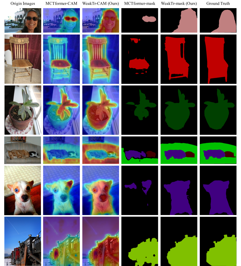
Figure 8: Comparison of the class activation maps (CAM) on the PASCAL VOC 2012 $train$ set.

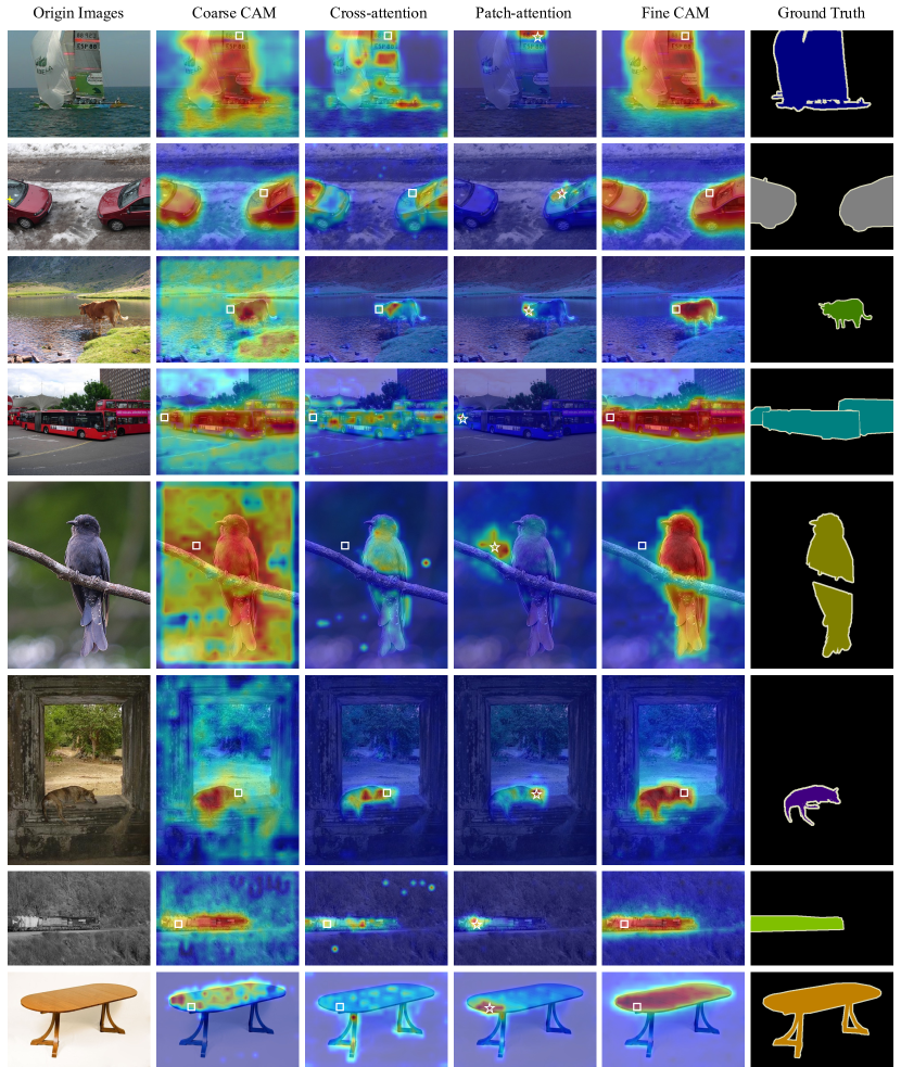
Figure 9: The coarse CAM, the cross-attention, the patch-attention, and the fine CAM results on the PASCAL VOC 2012 $train$ set. We use “$\star$” to denote the query points for the patch-attention. We also use “$\square$” to indicate the position of query points on the coarse CAM, the cross-attention, and the fine CAM.

Semantic Segmentation Results

We provide the more qualitative segmentation visualization results on the PASCAL VOC 2012 $val$ set in Fig. 10 and the COCO 2014 $val$ set in Fig. 11. We present the origin images, our WeakTr segmentation results, and the ground truth (GT). We can observe that for both indoor and outdoor scenes, our WeakTr can provide well-defined segmentation results. Especially for the more complex scenes in the COCO14 dataset, our WeakTr can also give reasonable segmentation results. At the same time, WeakTr also performs well when dealing with obscured objects. The segmentation results demonstrate that WeakTr’s online retraining with a gradient clipping decoder can effectively utilize CAM seeds to train the plain ViT-based segmentation network. It also demonstrates that plain ViT-based WSSS has great potential.

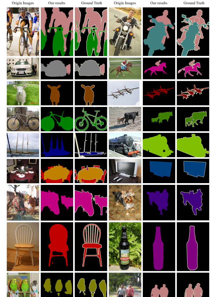
Figure 10: Segmentation visualization results on the PASCAL VOC 2012 $val$ set.

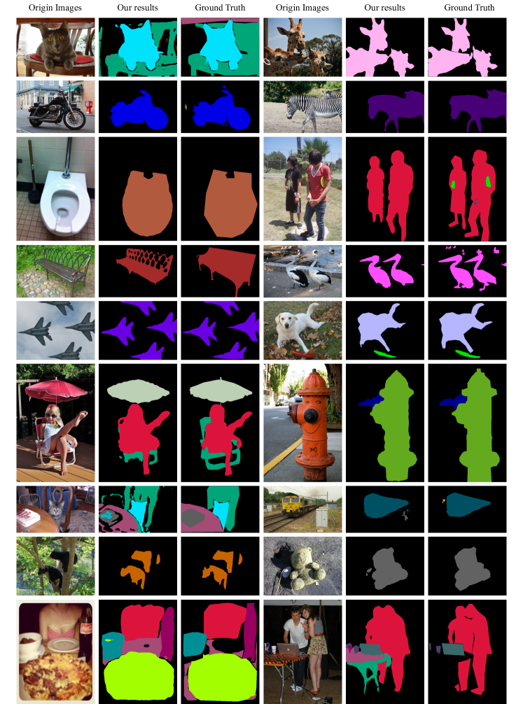
Figure 11: Segmentation visualization results on the COCO 2014 $val$ set.

References

- [1] Jiwoon Ahn, Sunghyun Cho, and Suha Kwak. Weakly supervised learning of instance segmentation with inter-pixel relations. In Proceedings of the IEEE/CVF conference on computer vision and pattern recognition, pages 2209–2218, 2019.
- [2] Jiwoon Ahn and Suha Kwak. Learning pixel-level semantic affinity with image-level supervision for weakly supervised semantic segmentation. In Proceedings of the IEEE conference on computer vision and pattern recognition, pages 4981–4990, 2018.
- [3] Eric Arazo, Diego Ortego, Paul Albert, Noel O’Connor, and Kevin McGuinness. Unsupervised label noise modeling and loss correction. In International conference on machine learning, pages 312–321. PMLR, 2019.
- [4] Yu-Ting Chang, Qiaosong Wang, Wei-Chih Hung, Robinson Piramuthu, Yi-Hsuan Tsai, and Ming-Hsuan Yang. Weakly-supervised semantic segmentation via sub-category exploration. In Proceedings of the IEEE/CVF Conference on Computer Vision and Pattern Recognition, pages 8991–9000, 2020.
- [5] Liyi Chen, Weiwei Wu, Chenchen Fu, Xiao Han, and Yuntao Zhang. Weakly supervised semantic segmentation with boundary exploration. In European Conference on Computer Vision, pages 347–362. Springer, 2020.
- [6] Liang-Chieh Chen, George Papandreou, Iasonas Kokkinos, Kevin Murphy, and Alan L Yuille. Deeplab: Semantic image segmentation with deep convolutional nets, atrous convolution, and fully connected crfs. IEEE transactions on pattern analysis and machine intelligence, 40(4):834–848, 2017.
- [7] Qi Chen, Lingxiao Yang, Jian-Huang Lai, and Xiaohua Xie. Self-supervised image-specific prototype exploration for weakly supervised semantic segmentation. In Proceedings of the IEEE/CVF Conference on Computer Vision and Pattern Recognition, pages 4288–4298, 2022.
- [8] Jia Deng, Wei Dong, Richard Socher, Li-Jia Li, Kai Li, and Li Fei-Fei. Imagenet: A large-scale hierarchical image database. In 2009 IEEE conference on computer vision and pattern recognition, pages 248–255. Ieee, 2009.
- [9] Alexey Dosovitskiy, Lucas Beyer, Alexander Kolesnikov, Dirk Weissenborn, Xiaohua Zhai, Thomas Unterthiner, Mostafa Dehghani, Matthias Minderer, Georg Heigold, Sylvain Gelly, et al. An image is worth 16x16 words: Transformers for image recognition at scale. arXiv preprint arXiv:2010.11929, 2020.
- [10] Mark Everingham, Luc Van Gool, Christopher KI Williams, John Winn, and Andrew Zisserman. The pascal visual object classes (voc) challenge. International journal of computer vision, 88(2):303–338, 2010.
- [11] Jiapei Feng, Xinggang Wang, and Wenyu Liu. Deep graph cut network for weakly-supervised semantic segmentation. Science China Information Sciences, 64(3):1–12, 2021.
- [12] Wei Gao, Fang Wan, Xingjia Pan, Zhiliang Peng, Qi Tian, Zhenjun Han, Bolei Zhou, and Qixiang Ye. Ts-cam: Token semantic coupled attention map for weakly supervised object localization. In Proceedings of the IEEE/CVF International Conference on Computer Vision, pages 2886–2895, 2021.
- [13] Bo Han, Quanming Yao, Xingrui Yu, Gang Niu, Miao Xu, Weihua Hu, Ivor Tsang, and Masashi Sugiyama. Co-teaching: Robust training of deep neural networks with extremely noisy labels. Advances in neural information processing systems, 31, 2018.
- [14] Bharath Hariharan, Pablo Arbeláez, Lubomir Bourdev, Subhransu Maji, and Jitendra Malik. Semantic contours from inverse detectors. In 2011 international conference on computer vision, pages 991–998. IEEE, 2011.
- [15] Qibin Hou, PengTao Jiang, Yunchao Wei, and Ming-Ming Cheng. Self-erasing network for integral object attention. Advances in Neural Information Processing Systems, 31, 2018.
- [16] Zilong Huang, Xinggang Wang, Jiasi Wang, Wenyu Liu, and Jingdong Wang. Weakly-supervised semantic segmentation network with deep seeded region growing. In Proceedings of the IEEE conference on computer vision and pattern recognition, pages 7014–7023, 2018.
- [17] Peng-Tao Jiang, Yuqi Yang, Qibin Hou, and Yunchao Wei. L2g: A simple local-to-global knowledge transfer framework for weakly supervised semantic segmentation. In Proceedings of the IEEE/CVF Conference on Computer Vision and Pattern Recognition, pages 16886–16896, 2022.
- [18] Alexander Kolesnikov and Christoph H Lampert. Seed, expand and constrain: Three principles for weakly-supervised image segmentation. In European conference on computer vision, pages 695–711. Springer, 2016.
- [19] Philipp Krähenbühl and Vladlen Koltun. Efficient inference in fully connected crfs with gaussian edge potentials. Advances in neural information processing systems, 24, 2011.
- [20] Hyeokjun Kweon, Sung-Hoon Yoon, Hyeonseong Kim, Daehee Park, and Kuk-Jin Yoon. Unlocking the potential of ordinary classifier: Class-specific adversarial erasing framework for weakly supervised semantic segmentation. In Proceedings of the IEEE/CVF International Conference on Computer Vision, pages 6994–7003, 2021.
- [21] Jungbeom Lee, Eunji Kim, and Sungroh Yoon. Anti-adversarially manipulated attributions for weakly and semi-supervised semantic segmentation. In Proceedings of the IEEE/CVF Conference on Computer Vision and Pattern Recognition, pages 4071–4080, 2021.
- [22] Jungbeom Lee, Seong Joon Oh, Sangdoo Yun, Junsuk Choe, Eunji Kim, and Sungroh Yoon. Weakly supervised semantic segmentation using out-of-distribution data. In Proceedings of the IEEE/CVF Conference on Computer Vision and Pattern Recognition, pages 16897–16906, 2022.
- [23] Jungbeom Lee, Jihun Yi, Chaehun Shin, and Sungroh Yoon. Bbam: Bounding box attribution map for weakly supervised semantic and instance segmentation. In Proceedings of the IEEE/CVF conference on computer vision and pattern recognition, pages 2643–2652, 2021.
- [24] Seungho Lee, Minhyun Lee, Jongwuk Lee, and Hyunjung Shim. Railroad is not a train: Saliency as pseudo-pixel supervision for weakly supervised semantic segmentation. In Proceedings of the IEEE/CVF conference on computer vision and pattern recognition, pages 5495–5505, 2021.
- [25] Ruiwen Li, Zheda Mai, Chiheb Trabelsi, Zhibo Zhang, Jongseong Jang, and Scott Sanner. Transcam: Transformer attention-based cam refinement for weakly supervised semantic segmentation. arXiv preprint arXiv:2203.07239, 2022.
- [26] Yi Li, Yiqun Duan, Zhanghui Kuang, Yimin Chen, Wayne Zhang, and Xiaomeng Li. Uncertainty estimation via response scaling for pseudo-mask noise mitigation in weakly-supervised semantic segmentation. In Proceedings of the AAAI Conference on Artificial Intelligence, volume 36, pages 1447–1455, 2022.
- [27] Chen Liang-Chieh, George Papandreou, Iasonas Kokkinos, Kevin Murphy, and Alan Yuille. Semantic image segmentation with deep convolutional nets and fully connected crfs. In International Conference on Learning Representations, 2015.
- [28] Tsung-Yi Lin, Michael Maire, Serge Belongie, James Hays, Pietro Perona, Deva Ramanan, Piotr Dollár, and C Lawrence Zitnick. Microsoft coco: Common objects in context. In European conference on computer vision, pages 740–755. Springer, 2014.
- [29] Ilya Loshchilov and Frank Hutter. Decoupled weight decay regularization. arXiv preprint arXiv:1711.05101, 2017.
- [30] Zhiliang Peng, Wei Huang, Shanzhi Gu, Lingxi Xie, Yaowei Wang, Jianbin Jiao, and Qixiang Ye. Conformer: Local features coupling global representations for visual recognition. In Proceedings of the IEEE/CVF International Conference on Computer Vision, pages 367–376, 2021.
- [31] Mengye Ren, Wenyuan Zeng, Bin Yang, and Raquel Urtasun. Learning to reweight examples for robust deep learning. In International conference on machine learning, pages 4334–4343. PMLR, 2018.
- [32] Herbert Robbins and Sutton Monro. A stochastic approximation method. The annals of mathematical statistics, pages 400–407, 1951.
- [33] Simone Rossetti, Damiano Zappia, Marta Sanzari, Marco Schaerf, and Fiora Pirri. Max pooling with vision transformers reconciles class and shape in weakly supervised semantic segmentation. In European Conference on Computer Vision, pages 446–463. Springer, 2022.
- [34] Lixiang Ru, Bo Du, Yibing Zhan, and Chen Wu. Weakly-supervised semantic segmentation with visual words learning and hybrid pooling. International Journal of Computer Vision, 130(4):1127–1144, 2022.
- [35] Lixiang Ru, Heliang Zheng, Yibing Zhan, and Bo Du. Token contrast for weakly-supervised semantic segmentation. arXiv preprint arXiv:2303.01267, 2023.
- [36] Olga Russakovsky, Jia Deng, Hao Su, Jonathan Krause, Sanjeev Satheesh, Sean Ma, Zhiheng Huang, Andrej Karpathy, Aditya Khosla, Michael Bernstein, et al. Imagenet large scale visual recognition challenge. International journal of computer vision, 115(3):211–252, 2015.
- [37] Tong Shen, Guosheng Lin, Lingqiao Liu, Chunhua Shen, and Ian Reid. Weakly supervised semantic segmentation based on co-segmentation. In BMVC, 2017.
- [38] Chunfeng Song, Yan Huang, Wanli Ouyang, and Liang Wang. Box-driven class-wise region masking and filling rate guided loss for weakly supervised semantic segmentation. In Proceedings of the IEEE/CVF Conference on Computer Vision and Pattern Recognition, pages 3136–3145, 2019.
- [39] Andreas Steiner, Alexander Kolesnikov, Xiaohua Zhai, Ross Wightman, Jakob Uszkoreit, and Lucas Beyer. How to train your vit? data, augmentation, and regularization in vision transformers. arXiv preprint arXiv:2106.10270, 2021.
- [40] Robin Strudel, Ricardo Garcia, Ivan Laptev, and Cordelia Schmid. Segmenter: Transformer for semantic segmentation. In Proceedings of the IEEE/CVF International Conference on Computer Vision, pages 7262–7272, 2021.
- [41] Yukun Su, Ruizhou Sun, Guosheng Lin, and Qingyao Wu. Context decoupling augmentation for weakly supervised semantic segmentation. In Proceedings of the IEEE/CVF international conference on computer vision, pages 7004–7014, 2021.
- [42] Kunyang Sun, Haoqing Shi, Zhengming Zhang, and Yongming Huang. Ecs-net: Improving weakly supervised semantic segmentation by using connections between class activation maps. In Proceedings of the IEEE/CVF International Conference on Computer Vision, pages 7283–7292, 2021.
- [43] Hugo Touvron, Matthieu Cord, Matthijs Douze, Francisco Massa, Alexandre Sablayrolles, and Hervé Jégou. Training data-efficient image transformers & distillation through attention. In International Conference on Machine Learning, pages 10347–10357. PMLR, 2021.
- [44] Yude Wang, Jie Zhang, Meina Kan, Shiguang Shan, and Xilin Chen. Self-supervised equivariant attention mechanism for weakly supervised semantic segmentation. In Proceedings of the IEEE/CVF Conference on Computer Vision and Pattern Recognition, pages 12275–12284, 2020.
- [45] Yunchao Wei, Jiashi Feng, Xiaodan Liang, Ming-Ming Cheng, Yao Zhao, and Shuicheng Yan. Object region mining with adversarial erasing: A simple classification to semantic segmentation approach. In Proceedings of the IEEE conference on computer vision and pattern recognition, pages 1568–1576, 2017.
- [46] Yunchao Wei, Xiaodan Liang, Yunpeng Chen, Xiaohui Shen, Ming-Ming Cheng, Jiashi Feng, Yao Zhao, and Shuicheng Yan. Stc: A simple to complex framework for weakly-supervised semantic segmentation. IEEE transactions on pattern analysis and machine intelligence, 39(11):2314–2320, 2016.
- [47] Zifeng Wu, Chunhua Shen, and Anton Van Den Hengel. Wider or deeper: Revisiting the resnet model for visual recognition. Pattern Recognition, 90:119–133, 2019.
- [48] Jinheng Xie, Xianxu Hou, Kai Ye, and Linlin Shen. Clims: Cross language image matching for weakly supervised semantic segmentation. In Proceedings of the IEEE/CVF Conference on Computer Vision and Pattern Recognition, pages 4483–4492, 2022.
- [49] Lian Xu, Wanli Ouyang, Mohammed Bennamoun, Farid Boussaid, Ferdous Sohel, and Dan Xu. Leveraging auxiliary tasks with affinity learning for weakly supervised semantic segmentation. In Proceedings of the IEEE/CVF International Conference on Computer Vision, pages 6984–6993, 2021.
- [50] Lian Xu, Wanli Ouyang, Mohammed Bennamoun, Farid Boussaid, and Dan Xu. Multi-class token transformer for weakly supervised semantic segmentation. In Proceedings of the IEEE/CVF Conference on Computer Vision and Pattern Recognition, pages 4310–4319, 2022.
- [51] Sung-Hoon Yoon, Hyeokjun Kweon, Jegyeong Cho, Shinjeong Kim, and Kuk-Jin Yoon. Adversarial erasing framework via triplet with gated pyramid pooling layer for weakly supervised semantic segmentation. In European Conference on Computer Vision, pages 326–344. Springer, 2022.
- [52] Dong Zhang, Hanwang Zhang, Jinhui Tang, Xian-Sheng Hua, and Qianru Sun. Causal intervention for weakly-supervised semantic segmentation. Advances in Neural Information Processing Systems, 33:655–666, 2020.
- [53] Fei Zhang, Chaochen Gu, Chenyue Zhang, and Yuchao Dai. Complementary patch for weakly supervised semantic segmentation. In Proceedings of the IEEE/CVF International Conference on Computer Vision, pages 7242–7251, 2021.
- [54] Bolei Zhou, Aditya Khosla, Agata Lapedriza, Aude Oliva, and Antonio Torralba. Learning deep features for discriminative localization. In Proceedings of the IEEE conference on computer vision and pattern recognition, pages 2921–2929, 2016.