Exactly solvable models of nonlinear extensions of the Schrödinger equation

Abstract

A method is presented to construct exactly solvable nonlinear extensions of the Schrödinger equation. The method explores a correspondence which can be established under certain conditions between exactly solvable ordinary Schrödinger equations and exactly solvable nonlinear theories. We provide several examples illustrating the method. We rederive well-known soliton solutions and find new exactly solvable nonlinear theories in various space dimensions which, to the best of our knowledge, have not yet been discussed in literature. Our method can be used to construct further nonlinear theories and generalized to relativistic soliton theories, and may have many applications.

I Introduction

It is “quite a rarity in the world of nonlinear differential equations” to encounter exact analytic solutions Shifman:2012zz . While some exact solutions of nonlinear theories are known, see for instance tHooft:1974kcl ; Polyakov:1974ek ; BialynickiBirula:1976zp ; BialynickiBirula:1979dp ; Oficjalski:1978 ; Zakharov-Shabat , the above quote from Ref. Shifman:2012zz nicely illustrates that in general they are rare. The goal of this work is to present a method allowing one to construct systematically exactly solvable nonlinear theories. We will focus on a specific class of nonlinear differential equations, namely on nonlinear extensions of the Schrödinger equation (NSE). The ordinary Schrödinger equation (SE) of nonrelativistic quantum mechanics is, of course, linear. But its nonlinear extensions have received considerable attention in literature and have numerous applications in a variety of contexts BialynickiBirula:1976zp ; BialynickiBirula:1979dp ; Oficjalski:1978 ; Zakharov-Shabat ; Rosen:1969ay ; Hudson:2017xug ; Belendryasova:2021jgs ; Gross ; Pitaevskii ; Lieb-Liniger:1963 ; Askaryan ; Talanov ; Chiao ; Kelley:1965 ; Tsuzuki:1971 ; Konotop:2004 ; Karpiuk:2012 ; dark-soliton-a ; dark-soliton-b ; Yefsah:2013 ; Peregrine ; rogue-ocean ; Wang:2020mjt ; rogue-optical ; Guth:2014hsa ; Kormos:2010 ; Beg:1984yh ; Namjoo:2017nia ; Weinstein:1983 ; Alvarez:1997ma ; Serkin-Hasegawa:2000 ; Blas:2015hro ; Biondini:2015pnf ; Koch:2022 .

In this work, we will show that under certain circumstances it is possible, starting from a known exact analytic ground state solution of a quantum mechanical problem, to construct an exactly solvable nonlinear theory. We will illustrate the method by providing several examples. In each case, the starting point is an exactly solvable quantum problem described by an ordinary SE like the harmonic oscillator, Coulomb problem, and other examples. As a result, we will derive nonlinear theories which have exact analytic solutions. In two of the cases, we will rederive well-known soliton solutions. In several other cases we will present exactly solvable NSEs which have not been discussed in literature before to the best of our knowledge. The method can be explored to construct systematically further exactly solvable nonlinear theories and can be generalized to relativistic theories.

Besides being of immense interest for their own sake, exactly solvable NSEs can provide useful toy models and theoretical test grounds in many situations. For instance, the availability of exact analytic solutions of nonlinear theories can be used to effectively test numerical methods for nonlinear partial differential equations. The numerous applications of NSE theories range from particle physics Rosen:1969ay ; Hudson:2017xug ; Belendryasova:2021jgs , to many body systems and propagation of light through nonlinear media Gross ; Pitaevskii ; Lieb-Liniger:1963 ; Askaryan ; Talanov ; Chiao ; Kelley:1965 ; Tsuzuki:1971 ; Konotop:2004 ; Karpiuk:2012 ; dark-soliton-a ; dark-soliton-b ; Yefsah:2013 , to descriptions of rogue waves in oceans or optics Peregrine ; rogue-ocean ; Wang:2020mjt ; rogue-optical , to cosmological models Guth:2014hsa . NSEs emerge naturally in the context of the transition from relativistic quantum field theories to nonrelativistic domains Kormos:2010 ; Beg:1984yh ; Namjoo:2017nia and play an important role in mathematical physics Weinstein:1983 ; Alvarez:1997ma ; Serkin-Hasegawa:2000 ; Blas:2015hro ; Biondini:2015pnf ; Koch:2022 .

Another important application of studies of NSE is to provide frameworks for experimental tests of the linearity of quantum mechanics. Different schemes have been proposed Weinberg:1989cm ; Kaplan-Rajendran and used to establish upper limits for nonlinear behavior in quantum mechanics based on neutron interferometry Shull:1980zz ; Gahler:1981zz , measurements in quantum bound states Bollinger:1989zz ; Chupp ; Walsworth:1990zz ; Majumder:1990zz , or Ramsey interferometry of vibrational modes of trapped ions Broz:2022aea . So far, no deviations from linear behavior have been observed, and it is of importance to establish more stringent experimental limits.

This work is organized as follows. In Sec. II, we introduce the notation and present the method to construct an analytically solvable NSE based on an analytically solvable SE. In Secs. III and IV, we explore the exactly solvable quantum harmonic oscillator to rederive a NSE describing a free or trapped Gausson in any number of space dimensions which has been encountered previously, independently in different theoretical settings. In Sec. V, we will rederive the well-known one-dimensional $1/\cosh$-soliton and generalize it to any number of dimensions in Sec. VI. The latter as well as the examples presented subsequently have not been discussed in literature before to the best of our knowledge and constitute novel results. This includes the exactly solvable NSE with an arbitrary power-like nonlinearity in Sec. VII and the NSE derived from a special case of the Rosen-Morse potential in Sec. VIII. In Sec. IX, we construct an interesting NSE based on an exactly solvable potential which contains the $\delta$-function potential as a limiting case. Our last example is an NSE derived from the exactly solvable Coulomb potential. Some of these examples are formulated in $N=1$ or $N=3$ dimensions, but several of them are formulated for general $N$. Our conclusions are presented in Sec. XI. The Appendix A contains technical details on an interesting limiting situation.

II Construction of exactly solvable NSEs

Let us begin with a remark regarding notation. In the NSE literature, often a unit system is used with $\hbar=1$ and many authors consider a particle of unit mass $m=1$ or set $2m=1$. In this work, we will explicitly use SI units and keep all physical constants in the equations. This will allow the reader to implement her or his preferred notation.

The starting point is ordinary quantum mechanics in $N$ space dimensions of a nonrelativistic spin-0 particle of mass $m$ moving in a potential $U(\vec{x})$ which is described by the linear Schrödinger equation (SE)

$$i\hbar\,\frac{\partial\Psi(t,\vec{x})}{\partial t}=-\,\frac{\hbar^{2}}{2m}\,\bigtriangleup\Psi(t,\vec{x})+U(\vec{x})\,\Psi(t,\vec{x})\,.$$ (1)

We shall assume the potential to be spherically symmetric such that $U(\vec{x})=U(r)$ with $r=|\vec{x}|$ for $N\geq 2$ dimensions. For $N=1$, we shall assume the potential $U(x)$ to be even. The $N$-dimensional Laplace operator is given by

$$\bigtriangleup=\frac{1}{r^{N-1}}\,\frac{\partial}{\partial r}\,r^{N-1}\,\frac{\partial}{\partial r}+\dots=\frac{\partial^{2}}{\partial r^{2}}+\frac{N-1}{r}\,\frac{\partial}{\partial r}+\dots\;\;$$ (2)

where, for $N\geq 2$, the dots indicate derivatives with respect to angular variables which will not be needed because we will focus exclusively on ground state wave functions depending solely on $r$ for a spherically symmetric potential. The space dimension $N$ will always be clear from the context.

Let the potential in Eq. (1) be such that it admits at least one bound state. We denote the ground state energy by $E_{0}$ and the ground state wave function by

$$\Psi_{0}(t,\vec{x})=c_{0}\,\phi_{0}(r)\,e^{-iE_{0}t/\hbar}$$ (3)

with the normalization $\int d^{N}r\,|\Psi_{0}(\vec{x},t)|^{2}=1$. Due to the symmetry of the potential, the spatial part of $\Psi_{0}(t,\vec{x})$ is described by a radial function $\phi_{0}(r)$ for $N\geq 2$ space dimensions. For $N=1$, the wave function $\phi_{0}(x)$ is even. For the following, it will be convenient to choose the phase and define the normalization constant $c_{0}>0$ in Eq. (3) such that

$$0\leq\phi_{0}(r)\leq 1\,,\quad\phi_{0}(0)=1\,.$$ (4)

After these preparations, we are in the position to present the method. If the quantum mechanical problem in Eq. (1) can be solved analytically, then, depending on the properties of the radial function $\phi_{0}(r)$, it may be possible to invert $\phi_{0}(r)$ and find a function $F$ such that the potential can be expressed as

$$U(r)=F[\Psi^{\ast}\Psi]\biggl{|}_{\Psi=\Psi_{0}(t,\vec{x})}\,.$$ (5)

If this step can be carried out, then $F$ will in general be a nonlinear function of the wave function $\Psi$. This allows us to rewrite the SE in Eq. (1) in terms of a nonlinear extension of the Schrödinger equation (NSE) as follows

$$i\hbar\,\frac{\partial\Psi}{\partial t}=-\,\frac{\hbar^{2}}{2m}\,\bigtriangleup\Psi+F[\Psi^{\ast}\Psi]\,\Psi\,.$$ (6)

Notice that it is convenient to choose $\Psi^{\ast}\Psi$ as variable of the nonlinear function in Eq. (5) because in this way the NSE (6) is linear with respect to the phase of $\Psi$ which carries the information about the time dependence.

The NSE (6) has the exact, analytically known solution given by Eq. (3) which corresponds to a stationary soliton solution in the corresponding nonrelativistic nonlinear theory. A soliton traveling with a constant velocity $\vec{v}$ can be obtained by applying a Galilean boost to Eq. (3) as follows

$$\Psi(t,\vec{x})=c_{0}\,\phi_{0}(\vec{x}-\vec{v}t)\,e^{i(m\vec{v}\cdot\vec{x}-\frac{1}{2}m\vec{v}^{2}t-E_{0}t)/\hbar}\,.$$ (7)

The crucial step in this construction is the derivation of the function $F[\Psi^{\ast}\Psi]$. For a spherically symmetric potential $U(\vec{x})=U(r)$ in $N\geq 2$ (or even potential $U(x)$ in $N=1$), it may be possible to carry out this step if $\phi_{0}(r)$ is monotonously decreasing and an inverse function $\phi_{0}^{-1}$ exists such that $\phi_{0}^{-1}[\phi_{0}(r)]=r$ (analogously for $N=1$). In our context, it will be important that this crucial step can be carried out analytically which ultimately depends on the properties of the potential.

In the following sections, we will discuss examples to illustrate the method. Hereby, we will focus on the construction of exactly solvable NSEs with analytic solutions. Such exactly solvable nonlinear theories are of interest for their own sake and may have interesting applications. In principle, further work is required to establish that a solution of a NSE of the type (7) can be considered a soliton in the strict mathematical sense. For that it would be important to show, for instance, that two such solutions can scatter off each other and will preserve their shapes long before and long after the scattering process. Such investigations are beyond the scope of this work, but have been carried out in literature in some cases and we shall refer to them in the following.

III $N$-dimensional logarithmic nonlinear theory, the free Gausson

As a first example, we consider the harmonic oscillator in $N$-dimensional space. The system is defined by the SE in Eq. (1) with a harmonic potential

$$U(r)=\frac{1}{2}\,m\,\Omega^{2}\,r^{2}\,.$$ (8)

The ground state energy and wave function are given by

$$\Psi_{0}(t,\vec{x})=c_{0}\,\phi_{0}(r)\,e^{-iE_{0}t/\hbar},\quad\phi_{0}(r)=e^{-r^{2}/b^{2}},\quad b=\sqrt{\frac{2\hbar}{m\Omega}}\,,\quad c_{0}=\biggl{(}\frac{m\Omega}{\pi\hbar}\biggr{)}^{\!N/4}\,,\quad E_{0}=\frac{1}{2}\,N\,\hbar\Omega\,.$$ (9)

Inverting the wave function as

$$r^{2}=-\frac{\hbar}{m\Omega}\;\ln\biggl{(}\frac{|\Psi_{0}(t,\vec{x})|^{2}}{|c_{0}|^{2}}\biggr{)}\,\$$ (10)

we can rewrite the harmonic potential as

$$U(r)=\frac{1}{2}\,m\Omega^{2}r^{2}=-\frac{\hbar\Omega}{2}\;\ln\biggl{(}\frac{|\Psi_{0}(t,\vec{x})|^{2}}{|c_{0}|^{2}}\biggr{)}\,.$$ (11)

In this way, we derive the NSE (6) with a logarithmic nonlinear term $F[\Psi^{\ast}\Psi]$ defined as follows

$$F\bigl{[}\Psi^{\ast}\Psi\bigr{]}=-A\,\ln\bigl{(}B\,|\Psi|^{2}\bigr{)}\,,\quad A=\frac{\hbar\Omega}{2},\quad B=\frac{1}{|c_{0}|^{2}}\,.$$ (12)

The exactly solvable NSE in Eqs. (6, 12) with the analytic solution (9) is known as the nonrelativistic Gausson, and was studied in detail in BialynickiBirula:1979dp ; BialynickiBirula:1976zp ; Oficjalski:1978 including relativistic formulations. Previously, these solutions were encountered in $N=3$ dimensions in studies of relativistic theories invariant under space-time dilatations Rosen:1969ay . Much later, Gaussons were rediscovered in a study of the energy-momentum tensor where point-like particles were “smeared out” to simulate an internal structure Hudson:2017xug . Recently, relativistic one-dimensional Gaussons were studied in Belendryasova:2021jgs .

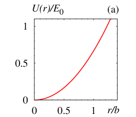
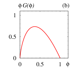
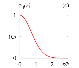
Figure 1: (a) The harmonic oscillator potential $U(r)$ in units of ground state energy $E_{0}$ as a function of $r$ in units of $b=\sqrt{2\hbar/(m\Omega)}$ in the 3-dimensional case. (b) The nonlinear term $\phi\,G(\phi)$ of the NSE defined in Eq. (13). (c) The radial part $\phi(r)$ of the ground state wave function of the SE with the potential in (a) and the soliton of the NSE defined by the nonlinear term in (b).

In Fig. 1, we show the potential of the SE, the nonlinear term of the NSE, and the radial part of the wave function (the potential and $\phi_{0}(r)$ of the harmonic oscillator are well known, but we include them for completeness and consistency with the following sections). It is convenient to display the potential in Fig. 1a in units of the ground state energy and $r$ in units of $b=\sqrt{2\hbar/(m\Omega)}$. The nonlinear term (12) is visualized as a function of the dimensionless variable $\phi$ as

$$F\bigl{[}\Psi^{\ast}\Psi\bigr{]}=A\,G\bigl{(}|\Psi|/c_{0}\bigr{)}\,,\quad G(\phi)=-{\rm ln}\,\phi^{2}.$$ (13)

Recalling the normalization and phase convention in Eq. (4), the variable $\phi$ satisfies $0\leq\phi\leq 1$. For $0<\phi<1$ the function $G(\phi)$ is positive. As $\phi\to 0$ the nonlinear term $G(\phi)$ diverges which reflects the growth of $U(r)$ for $r\to\infty$. However, the nonlinearity enters in Eqs. (6, 12) practically as $\phi\,G(\phi)$ which goes to zero for $\phi\to 0$ and $\phi\to 1$ assuming its maximum in between at $\phi=1/e$, i.e. at this point the nonlinearity in Eqs. (6, 12) is strongest, see Fig. 1b. The radial part $\phi_{0}(r)$ of respectively the ground state wave function of the ordinary SE and the soliton of the NSE is shown in Fig. 1c.

The solution (9) corresponds to a Gausson at rest. By applying the Galilean boost in Eq. (7) to the solution (9), we obtain a soliton traveling with constant velocity which preserves its shape. In our derivation, the shape-preserving traveling solution appears as a trivial consequence of Galilean invariance of the NSE in Eqs. (6, 12). As remarked in Sec. II, dedicated analyses are needed to show that such shape-preserving solutions can scatter off each other and asymptotically (i.e. long before and long after the scattering event) preserve their shapes. In the case of the Gausson solution,this was shown in BialynickiBirula:1979dp ; BialynickiBirula:1976zp . Noteworthy is the existence of a “resonance region” in which the scattering can be inelastic and the collision of two Gaussons can produce a final state with three Gaussons Oficjalski:1978 .

IV Theory of a Gausson trapped in a harmonic potential

The steps carried out in Sec. III can be performed also for a “part” of the potential leading to the NSE of a Gausson trapped in the “remaining part” of the harmonic potential. For definiteness, we will consider $N=3$ space dimensions, but a generalization to other space dimensions $N$ is straightforward and analogous to Sec. III.

For that, let us consider the harmonic potential $U(r)=\frac{1}{2}\,m\,\Omega_{1}^{2}\,r^{2}+\frac{1}{2}\,m\,\Omega_{2}^{2}\,r^{2}$ with $\Omega_{1}^{2}+\Omega_{2}^{2}=\Omega^{2}$. Now we choose the part $\frac{1}{2}\,m\,\Omega_{1}^{2}\,r^{2}$ of the potential to be left alone and reformulate the part $\frac{1}{2}\,m\,\Omega_{2}^{2}\,r^{2}$ in terms of the nonlinear theory as discussed in Sec. III. In this way, we obtain the following NSE

$$i\hbar\,\frac{\partial\Psi}{\partial t}=-\,\frac{\hbar^{2}}{2m}\,\bigtriangleup\Psi+U_{1}(r)\,\Psi+F_{2}\bigl{[}\Psi^{\ast}\Psi]\;\Psi\,,$$ (14)

where the potential $U_{1}(r)$, the nonlinear term $F_{2}\bigl{[}\Psi^{\ast}\Psi]$ and the constants $A_{2}>0$ and $B_{2}>0$ are given by

$$U_{1}(r)=\frac{1}{2}\,m\,\Omega_{1}^{2}\,r^{2},\quad F_{2}\bigl{[}\Psi^{\ast}\Psi]=-A_{2}\,\ln\bigl{(}B_{2}\,\Psi^{\ast}\Psi\bigr{)}\,,\quad A_{2}=\frac{\hbar\Omega_{2}^{2}}{2\Omega},\quad B_{2}=\biggl{(}\frac{\pi\hbar}{m\Omega}\biggr{)}^{3/2}\,.$$ (15)

Let us recall that these results are specifically for $N=3$ space dimensions and the generalization to other dimensions is straight forward. The NSE given by Eqs. (14, 15) describes a Gausson trapped in the harmonic potential $U_{1}(r)=\frac{1}{2}\,m\,\Omega_{1}^{2}\,r^{2}$ with the analytic solution given by Eq. (9).

In the limit $\Omega_{1}\rightarrow\Omega$ and $\Omega_{2}\rightarrow 0$, the nonlinear theory (14, 15) reduces to the regular SE for a harmonic oscillator. In the limit $\Omega_{1}\rightarrow 0$ and $\Omega_{2}\rightarrow\Omega$, it reduces to the nonlinear theory of a free Gausson discussed in Sec. III.

V Nonlinear theory with a 1/cosh soliton in one-dimension

In our next example, we consider a one-dimensional quantum system described by the potential

$$U(x)=-\,\frac{\hbar^{2}}{m\,a^{2}}\frac{1}{\cosh^{2}{(x/a)}}\,,$$ (16)

where $a$ is a positive constant with the dimension of length. The ground state solution of the SE reads

$$\Psi_{0}(t,x)=c_{0}\,\phi_{0}(x)\,e^{-iE_{0}t/\hbar},\quad\phi_{0}(x)=\frac{1}{\cosh(x/a)}\,,\quad c_{0}=\frac{1}{\sqrt{2a}}\,,\quad E_{0}=-\frac{\hbar^{2}}{2m\,a^{2}}\,.$$ (17)

Using the method described in Sec. II, the wave function can be inverted and used to express the potential in terms of the ground state wave function as follows

$$U(x)=-\frac{2\hbar^{2}}{ma}\Psi^{\ast}_{0}(t,x)\Psi_{0}(t,x)\,.$$ (18)

The resulting analytically solvable NSE is then given by Eq. (6) with a particularly simple nonlinear term

$$F\bigl{[}\Psi^{\ast}\Psi\bigr{]}=-A\,|\Psi|^{2}\,,\quad A=\frac{2\hbar^{2}}{ma}\,.$$ (19)

The analytic solution (17) of the nonlinear theory (6, 19) is well known and was found in Ref. Zakharov-Shabat . The underlying NSE in $N=3$ is generally known as the Gross-Pitaevskii equation Gross ; Pitaevskii and has important applications to the description of interacting Bose gases. In $N=1$ dimensions, it is often referred to as the Lieb-Liniger model Lieb-Liniger:1963 . The wide range of applications of this nonlinear theory includes propagation of self-focusing laser beams in nonlinear media Askaryan ; Talanov ; Chiao ; Kelley:1965 , solitons in Bose condensates Tsuzuki:1971 ; Konotop:2004 ; Karpiuk:2012 ; dark-soliton-a ; dark-soliton-b and fermionic superfluids Yefsah:2013 , generation of ocean Peregrine ; rogue-ocean ; Wang:2020mjt and optical rogue-optical rogue waves, or cosmological axion models of nonrelativistic dark matter Guth:2014hsa . The NSE can be derived from, e.g., the nonrelativistic limit of the one-dimensional sinh-Gordon model Kormos:2010 , or the complex $\Phi^{4}$ theory Beg:1984yh ; Namjoo:2017nia . Suffice to say that this NSE is of great interest in mathematical physics Weinstein:1983 ; Alvarez:1997ma ; Serkin-Hasegawa:2000 ; Blas:2015hro ; Biondini:2015pnf ; Koch:2022 . In the case of solitons in Bose condensates, the sign of the nonlinearity is opposite to our result and the equation describes a “dark soliton” which corresponds to a depletion in the density in the Bose condensate Tsuzuki:1971 ; Konotop:2004 ; Karpiuk:2012 ; dark-soliton-a ; dark-soliton-b .

For completeness, we remark that the potential $U(x)$ in Eq. (16) is a special case of the Rosen-Morse potential Rosen-Morse:1932 and belongs to a wider class of potentials known as Natanzon potentials Natanzon:1979 . We postpone displaying the potential, nonlinear term, and wave function to the next section where we generalize the 1/cosh solution to an arbitrary number of dimensions $N$.

VI Nonlinear theory with a 1/cosh soliton in $N$ dimensions

The 1/cosh solitons exist also in $N>1$ dimensions, albeit the starting point is then a somewhat more complicated quantum mechanical potential which contains an additional term proportional to $(N-1)$ and is given by

$$U(r)=-\,\frac{\hbar^{2}}{ma^{2}}\frac{1}{\cosh^{2}{(r/a)}}-\,(N-1)\,\frac{\hbar^{2}}{2ma\,r}\,\tanh(r/a)$$ (20)

where $a$ is a positive constant with the dimension of length. Clearly, for $N=1$ we recover the potential of Sec. V. The ground state solution of the SE is given by

$$\Psi_{0}(t,\vec{x})=c_{0}(N)\,\phi_{0}(r)\,e^{-iE_{0}t/\hbar},\quad\phi_{0}(r)=\frac{1}{\cosh(r/a)}\,,\quad E_{0}=-\frac{\hbar^{2}}{2m\,a^{2}}\,,$$ (21)

and is exactly the same as in Sec. V except the normalization constant is now given by

$$c_{0}(N)=\sqrt{\frac{4^{N-1}\,\Gamma(N/2+1)}{(2^{N}-4)\,N\,(N-1)!\,\pi^{N/2}\zeta(N-1)a^{N}}}\,,\quad N>2\,.$$ (22)

In the case $N=2$, care is needed because the factor $(2^{N}-4)$ goes to zero while the $\zeta$-function $\zeta(N-1)$ diverges, but the product of these factors $(2^{N}-4)\,\zeta(N-1)\to 4\ln 2$ is finite such that $c_{0}(2)=1/(a\sqrt{2\pi\ln 2})$. For $N=1$ the formula (22) reproduces the normalization constant quoted in Sec. V in Eq. (17).

Inverting the wave function, the potential can be rewritten as

$$U(r)=A\,G\bigl{(}|\Psi_{0}(t,\vec{x})|/c_{0}|\bigr{)},\quad A=\frac{\hbar^{2}}{ma}\,,\quad G(\phi)=-\phi^{2}-\frac{1}{2}\,(N-1)\frac{\sqrt{1-\phi^{2}}}{\ln\bigl{(}1+\sqrt{1-\phi^{2}}\bigr{)}-\ln\phi}\,.$$ (23)

The resulting analytically solvable NSE is then given by Eq. (6) with the nonlinear function

$$F[\Psi^{\ast}\Psi]=A\>G\bigl{(}|\Psi/c_{0}|\bigr{)}$$ (24)

with $G(\phi)$ and $A$ defined in Eq. (23). The results are valid for any dimension $N$ including the one-dimensional case discussed in Sec. V. To the best of our knowledge, the solution for $N>1$ has not been discussed before in literature.

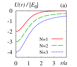
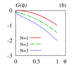
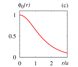
Figure 2: (a) The potential $U(r)$ in Eq. (20) in units of $|E_{0}|$ for $N=1,\,2,\,3$ dimensions. (b) The nonlinear term $G(\phi)$ defined in Eq. (23) for $N=1,\,2,\,3$ dimensions. (c) The radial part $\phi_{0}(r)=1/\cosh(r/a)$ of the ground state wave function which is the solution to the SE with the potential shown in (a) and the NSE with the nonlinear term shown in (b) for any dimension $N$.

In units of $|E_{0}|$, the potential has the shape $V(r)/|E_{0}|=-2/\cosh(y)^{2}-(N-1)\tanh(y)/y$ where $y=r/a$ and is depicted in Fig. 2a for $N=1,\,2,\,3$ dimensions. The function $G(\phi)$ defined in Eq. (23) is similarly shown for $N=1,\,2,\,3$ dimensions in Fig. 2b. Although the nonlinearity in (23) enters effectively as $\phi\,G(\phi)$, we merely plot $G(\phi)$ since in this case the nonlinear function vanishes for $\phi\to 0$ (in contrast to the nonlinearity in the Gausson case in Fig. 1b). In the limit $\phi\to 1$, the function $G(\phi)$ approaches the value $(-N-1)/2$. We see that the nonlinearity in this NSE has a very different shape and opposite sign compared to the nonlinearity of the Gausson discussed in Secs. III and IV. The radial wave function has the same 1/cosh shape in any dimension and is shown in Fig. 2c.

VII One-dimensional theory with a power-law nonlinearity $F[\Psi^{\ast}\Psi]=|\Psi^{\ast}\Psi|^{\lambda}$

In this section, we present an interesting variant of the NSE discussed in Sec. V. In a one-dimensional quantum system, we consider the potential

$$U(x)=-\,\frac{1+\lambda}{2\lambda^{2}}\,\frac{\hbar^{2}}{m\,a^{2}}\frac{1}{\cosh^{2}{(x/a)}}\,.$$ (25)

where $a>0$ has the dimension of length and $\lambda>0$ is dimensionless. The case $\lambda=1$ was discussed in Sec. V, and for $\lambda\to\infty$ we recover the free SE. For $0<\lambda<\infty$, the ground state solution of the SE with the potential (25) reads

$$\Psi_{0}(t,x)=c_{0}\,\phi_{0}(x)\,e^{-iE_{0}t/\hbar},\quad\phi_{0}(x)=\frac{1}{\cosh(x/a)^{1/\lambda}}\,,\quad c_{0}=\sqrt{\frac{\Gamma(1/2+1/\lambda)}{\sqrt{\pi}\,\Gamma(1/\lambda)\,a}}\,,\quad E_{0}=-\frac{1}{\lambda^{2}}\,\frac{\hbar^{2}}{2m\,a^{2}}\,.$$ (26)

Using the method described in Sec. II, the wave function can be inverted and used to express the potential in terms of the ground state wave function as follows

$$U(x)=-\,\frac{1+\lambda}{2\lambda^{2}}\,\frac{\hbar^{2}}{m\,a^{2}}\,\bigl{(}\phi_{0}^{\ast}(x)\phi_{0}(x)\bigr{)}^{\lambda}\,\,.$$ (27)

The resulting analytically solvable NSE is then given by Eq. (6) with with the power-law nonlinear term

$$F\bigl{[}\Psi^{\ast}\Psi\bigr{]}=A\,|\Psi|^{2\lambda}\,,\quad A=-\,\frac{1+\lambda}{2\lambda^{2}}\,\frac{2\hbar^{2}}{m\,a\,c_{0}^{2\lambda}}\,.$$ (28)

The constant $\lambda$ can be chosen to model any desired power-law nonlinearity proportional to $|\Psi|^{2\lambda}$.

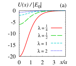
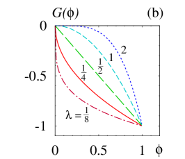
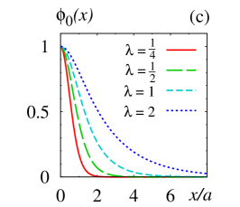
Figure 3: (a) The potential (25) in units of $|E_{0}|$, (b) the nonlinear term $G(\phi)=-\,\phi^{2\lambda}$ defined below Eq. (28), and (c) the solution $\phi_{0}(x)=1/\cosh(x/a)^{1/\lambda}$ of the SE with the potential in (a) and the NSE with the nonlinear term in (b) for different $0<\lambda\leq 2$.

In Fig. 3, we show the potential $U(x)$, the nonlinear term defined as $G(\phi)=-\,\phi^{2\lambda}$, and $\phi_{0}(x)$ for selected $\lambda$ values. As $\lambda$ increases, $U(x)$ becomes shallower and $G(\phi)$ more strongly peaked towards the region $\phi\to 1$. In absolute units, the spatial part of the soliton is $c_{0}\,\phi_{0}(x)$ and the normalization constant $c_{0}$ decreases as $\lambda$ increases. I.e., in the limit when $\lambda$ becomes large, the soliton decreases in the center and spreads out, i.e. it becomes delocalized. At the same time as $\lambda$ becomes large, the magnitude of the energy $E_{0}\propto 1/\lambda^{2}$ decreases. For $\lambda\to\infty$, we recover the free SE as the potential $U(x)\to 0$ in Eq. (25) and also the nonlinear term $F\bigl{[}\Psi^{\ast}\Psi\bigr{]}\to 0$ in Eq. (28). If we apply a Galilean boost according to (7) and take $\lambda\to\infty$, the solution is of course not normalizable and corresponds to a plane wave.

The opposite limit of small $\lambda$ is also interesting. The potential of the SE becomes deeper and $E_{0}$ becomes more negative. In the NSE, the magnitude of the nonlinear term increases (it becomes more negative) since $A$ is proportional to $1/\lambda^{2}$ in Eq. (28) and the soliton becomes more strongly localized. This picture remains correct for arbitrarily small, but non-zero $\lambda$. In the strict limit $\lambda\to 0$ the potential of the SE (and the nonlinear term of the NSE) become singular, the ground state energy $E_{0}\to-\,\infty$, while the ground state wave function becomes strongly localized and approaches $|\psi_{0}(x,t)|^{2}\to\delta(x)$. In Appendix A, we show that despite this extreme localization of the state for $\lambda\to 0$, Heisenberg’s uncertainty principle is always valid.

For completeness, we remark that the solution $\phi_{0}(r)=1/\cosh(r/a)^{1/\lambda}$ exists also in $N\geq 2$ dimensions for a generalized potential and a generalized nonlinearity which then both have additional structures proportional to $(N-1)$. The situation is similar to the case discussed in Sec. VI, and we refrain from showing the results.

VIII Example of a NSE from piecewise potential

Some exactly solvable quantum problems are given in terms of potentials which are defined piecewise. Our next example is of this type. We will see that it is possible to derive an NSE also in such a case. In a one-dimensional quantum system, we consider the potential given by

$$U(x)=\frac{\hbar^{2}}{2mL^{2}}\,\beta(\beta-1)\tan^{2}\left(\frac{x}{L}\right)\quad\mbox{for}\quad|x|<\frac{\pi\,L}{2}\;,$$ (29)

and infinite for $|x|\geq\pi\,L/2$ where $L$ is a positive parameter of dimension length and $\beta>1$ is dimensionless. The ground state solution of the SE with the potential (29) is for $|x|<\pi\,L/2$ given by

$$\Psi_{0}(t,x)=c_{0}\,\phi_{0}(x)\,e^{-iE_{0}t/\hbar},\quad\phi_{0}(x)=\biggl{(}\cos\frac{x}{L}\biggr{)}^{\beta},\quad c_{0}=\sqrt{\frac{\beta\,\Gamma(\beta)}{\sqrt{\pi}\,\Gamma(\beta+\tfrac{1}{2})L}}\,,\quad E_{0}=\frac{\hbar^{2}\beta}{2mL^{2}}$$ (30)

and zero elsewhere. The wave function can be inverted and used to express the potential in terms of $\phi_{0}(x)$ as follows

$$U(x)=\frac{\hbar^{2}}{2mL^{2}}\,\beta(\beta-1)\left(\phi_{0}(x)^{-2/\beta}-1\right)\quad\mbox{for}\quad|x|<\frac{\pi\,L}{2}\;.$$ (31)

The resulting analytically solvable NSE is then given by Eq. (6) with the nonlinear term defined as

$$F\bigl{[}\Psi^{\ast}\Psi\bigr{]}=A\,G\bigl{(}|\Psi/c_{0}|\bigr{)}\,,\quad G(\phi)=\beta(\beta-1)\left(\phi^{-2/\beta}-1\right),\quad A=\frac{\hbar^{2}}{2L^{2}m}\,.$$ (32)

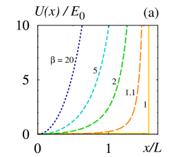
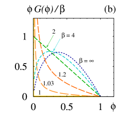
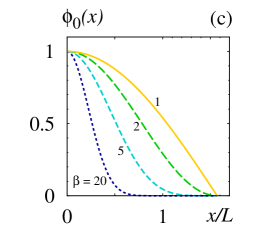
Figure 4: (a) The potential $U(x)$ in Eq. (29) in units of $|E_{0}|$ for selected values of $\beta$. The limiting case $\beta=1$ corresponds to the familiar square well potential. (b) The nonlinear term $\phi\,G(\phi)$ with $G(\phi)$ defined in Eq. (32) normalized with respect to the parameter $\beta$ to better illustrate the scaling in the large-$\beta$ limit. (c) The solution $\phi_{0}(x)=1/\cos(x/L)^{\beta}$ for selected values of $\beta$.

The potential, nonlinear term, and $\phi_{0}(x)$ are shown in Fig. 4 for selected values of $\beta$. For $\beta\to 1$, the potential (29) approaches the familiar infinite square well potential, while for $\beta\gg 1$, the potential becomes very steep, see Fig. 4a. In the limit $\beta\to 1$, also the nonlinear function has formally a “square well-type shape” with the properties (i) $G(\phi)=0$ for $\phi\neq 0$, and (ii) $G(\phi)\to\infty$ as $\phi\to 0$ as illustrated in Fig. 4b. However, although $\beta$ can be infinitesimally close to unity, the NSE can only be solved for $\beta>1$. In the limit of large $\beta$, the non-linear function grows with $\beta$. But when normalized with respect to $\beta$, the nonlinearity has the limit $\lim_{\beta\to\infty}\phi\,G(\phi)/\beta=-2\,\phi\,\ln\phi$, as depicted in Fig. 4b. As $\beta\to 1$, the solution $\phi_{0}(x)$ approaches the shape $\cos(x/L)$ familiar from the square well potential, while for $\beta\gg 1$ it becomes strongly localized, see Fig. 4c. In the limit $\beta\to\infty$, the function $\phi_{0}(x)\to 0$ for $x\neq 0$, and the normalized wave function takes the limit $\lim_{\beta\to\infty}|\psi_{0}(x,t)|^{2}=\delta(x)$. Despite the strong localization of the wave function for $\beta\to\infty$, Heisenberg’s uncertainty relation remains valid because the shrinking of the position uncertainty $\Delta x\to 0$ is accompanied by the corresponding spread of the momentum uncertainty $\Delta p\to\infty$. Notice also that $E_{0}$ diverges as $\beta$ grows. For any $\beta<\infty$ it is always $\Delta p\,\Delta x>\frac{1}{2}\,\hbar$, and the uncertainty relation becomes an equality in the limit $\beta\to\infty$. The situation is analog to the limit $\lambda\to 0$ in Sec. VII which is discussed in detail in App. A.

IX Nonlinear theory with $\delta$-function type limiting case

In this section, we consider the one-dimensional potential given by the expression

$$U(x,b_{0})=-\;\frac{\hbar^{2}b_{0}^{2}}{2am}\;\left[\frac{1}{\left(x^{2}+b_{0}^{2}\right){}^{3/2}}+\frac{1}{a\left(x^{2}+b_{0}^{2}\right)}\right]\,,$$ (33)

where $a>0$ and $b_{0}>0$ are constants with the dimension of length. The ground state solution of the ordinary SE with the potential in Eq. (33) is given by

$$\Psi_{0}(t,x)=c_{0}\phi_{0}(x)\,e^{-iE_{0}t/\hbar},\quad\phi_{0}(x)=\exp\biggl{(}\frac{b_{0}}{a}-\frac{\sqrt{x^{2}+b_{0}^{2}}}{a}\biggr{)},\quad E_{0}=-\,\frac{\hbar^{2}}{2a^{2}m}\,.$$ (34)

We could not find an analytic expression for the normalization constant $c_{0}$ valid in the general case, though it can be computed numerically if needed. The expression for $c_{0}$ is not of importance for the following. Notice that $\phi_{0}(0)=1$ in accordance with Eq. (4).

The radial function $\phi_{0}(x)$ can be inverted and the potential expressed as

$$U(x,b_{0})=\frac{\hbar^{2}}{2a^{2}m}\,G\bigl{(}\phi_{0}(x),b_{0}\bigr{)},\quad G(\phi,b_{0})=\frac{b_{0}^{2}}{a^{2}}\,\frac{1-\ln(e^{-b_{0}/a}\phi)}{\ln^{3}(e^{-b_{0}/a}\phi)}\,.$$ (35)

In this way, we obtain the exactly solvable NSE in Eq. (6) with the nonlinearity

$$F\bigl{[}\Psi^{\ast}\Psi\bigr{]}=A\,G\bigl{(}|\Psi|/c_{0},b_{0}\bigr{)}\,,\quad A=\frac{\hbar^{2}}{2m\,a^{2}}\,,$$ (36)

with $G(\phi,b_{0})$ defined in Eq. (35). The nonlinear theory (36) has the analytic solution (34) and can describe traveling solutions according to (7).

We defined the potential in Eq. (33) for $b_{0}>0$ and excluded the case $b_{0}=0$. But the limit $b_{0}\to 0$ can be taken, and it is indeed very interesting. In this limit, the potential (33) has the properties

(i) $$\;\;\lim_{b_{0}\to 0}U(x,b_{0})\;=\;0\quad{\rm for}\quad x\neq 0\,,$$

(ii) $$\int\limits_{-\infty}^{\infty}\!\!{\rm d}x\;U(x,b_{0})\;=\;-\frac{\hbar^{2}(2a+\pi b_{0})}{2a^{2}m}\quad{\rm for}\quad b_{0}\neq 0\,.$$ (37)

These are basically the defining equations for a $\delta$-function, i.e. in the limit that $b_{0}\to 0$, the potential reduces to the $\delta$-function potential

$$U(x)\equiv\lim_{b_{0}\to 0}U(x,b_{0})=-\frac{\hbar^{2}}{a\,m}\,\delta(x)\,,$$ (38)

while the wave function (34) reduces in this limit to the known solution of this familiar textbook potential, namely

$$\Psi_{0}(t,x)=c_{0}\,\phi_{0}(r)\,e^{-iE_{0}t/\hbar},\quad\phi_{0}(x)=\exp\biggl{(}-\frac{|x|}{a}\biggr{)},\quad c_{0}=\frac{1}{\sqrt{a}}\,,\quad E_{0}=-\,\frac{\hbar^{2}}{2a^{2}m}\,.$$ (39)

The formulation of the pertinent NSE must be performed with similar care. The nonlinear function (35) satisfies

$${\rm(i)} \lim_{b_{0}\to 0}G(\phi,b_{0})=0\quad{\rm for}\quad 0\leq\phi<1,$$

$${\rm(ii)} \int\limits_{0}^{1}{\rm d}\phi\;G(\phi,b_{0})=-\,\frac{1}{2}-\frac{b_{0}}{2a}-\frac{b_{0}^{2}}{2a^{2}}\,e^{b_{0}/a}\,\text{Ei}(-b_{0}/a)\quad{\rm for}\quad b_{0}>0,$$ (40)

where ${\rm Ei}(-y)=\int_{y}^{\infty}du\,e^{-u}/u$ denotes the exponential integral. The properties in Eq. (IX) define in the limit $b_{0}\to 0$ a $\delta$-function, this time with support at $\phi=1$, i.e.

$$\lim_{b_{0}\to 0}G(\phi,b_{0})=-\,\delta(1-\phi)\,,$$ (41)

with the convention that integrating a $\delta$-function up to a limit which coincides with its support yields $\int_{0}^{c}{\rm d}u\,\delta(u-c)=\frac{1}{2}$ for $c>0$. In this way, we find an unusual exactly solvable NSE, namely

$$i\hbar\,\frac{\partial\Psi}{\partial t}=-\,\frac{\hbar^{2}}{2m}\,\bigtriangleup\Psi-A\,\delta\bigl{(}1-|\Psi|/\sqrt{a}\bigr{)}\,,\quad A=\frac{\hbar^{2}}{2m\,a^{2}}\,.$$ (42)

The nonlinearity in this problem is nonzero only when the spatial part of the wave function $\phi(x)$ becomes unity. This is the case for the solution $\phi_{0}(x)$ in Eq. (39) (cf. Eq. (4) for conventions) only at $x=0$ corresponding to the only point where the limiting potential (38) is nonzero. The very presence of the singular nonlinearity in Eq. (42) can be verified only by integrating the (time-independent version of the) NSE in Eq. (42) over an infinitesimal interval $[-\epsilon,\,\epsilon]$ enclosing the point $x=0$, i.e. in very much the same way the singular potential (38) is treated in the ordinary SE.

In Fig. 5, we show the potential, nonlinear term and spatial part $\phi_{0}(x)$ for selected values of $b_{0}$. As the parameter $b_{0}$ decreases, the potential and nonlinear term become narrower and deeper as shown in Figs. 5a and 5b. The minimum of the potential in units of $|E_{0}|$ and the non-linear function are given by $U(0,b_{0})/|E_{0}|=G(1,b_{0})=-a/b_{0}-1$ and go to minus infinity for $b_{0}\to 0$. Both functions eventually approach the corresponding singular limits in Eqs. (38, 41) which cannot be depicted. The wave function $\phi_{0}(x)$ is regular in the limiting case $b_{0}\to 0$ and shown in Fig. 5c.

In the opposite limit $b_{0}\to\infty$, the potential $U(x,b_{0})\to E_{0}$ becomes a trivial constant, the non-linearity $G(\phi,b_{0})\to 0$. After a Galilean boost (7), the wave-function describes a non-renormalizable plane wave solution. In other words, we recover a free SE in the limit $b_{0}\to\infty$.

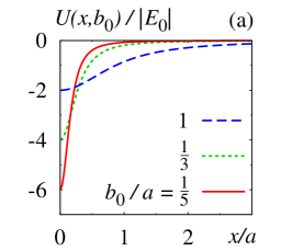
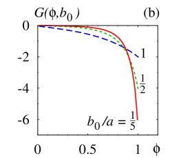
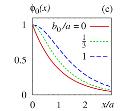
Figure 5: (a) The potential $U(x,b_{0})$ in Eq. (33) in units of $|E_{0}|$ for selected values of $b_{0}$. For $b_{0}\to 0$ the potential reduces to an attractive $\delta(x)$ potential. (b) The nonlinear term $G(\phi,b_{0})$ defined in Eq. (35) which becomes $-\,\delta(1-\phi)$ in the limit $b_{0}\to 0$. (c) The solution $\phi_{0}(x)$ for selected values of $b_{0}$ including the limit $b_{0}\to 0$.

X Three-dimensional nonlinear theory from Coulomb potential

As our final example, we choose another well-familiar analytically solvable quantum mechanical potential, namely the Coulomb potential in $N=3$ dimensions. The potential is given by

$$U(r)=-\,\frac{e^{2}}{4\pi\varepsilon_{0}}\,\frac{1}{r}=-\frac{\hbar^{2}}{a_{B}\,m}\,\frac{1}{r}$$ (43)

where $a_{B}=4\pi\varepsilon_{0}\hbar^{2}/(e^{2}m)=\hbar/(\alpha mc)$ denotes the Bohr radius, $m$ the reduced mass, and $\alpha$ the fine structure constant. The ground state energy and wave function are given by

$$\Psi_{0}(t,\vec{x})=c_{0}\,\phi_{0}(r)\,e^{-iE_{0}t/\hbar},\quad\phi_{0}(r)=\exp\biggl{(}-\frac{r}{a_{B}}\biggr{)},\quad c_{0}=\biggl{(}\frac{1}{\pi a^{3}_{B}}\biggr{)}^{\!1/2}\,,\quad E_{0}=-\,\frac{\hbar^{2}}{2a^{2}_{B}m}=-\frac{1}{2}\,\alpha^{2}\,mc^{2}\,.$$ (44)

This wave function can be inverted such that we obtain

$$r=-\frac{a_{B}}{2}\;\ln\biggl{(}\frac{|\Psi_{0}(t,\vec{x})|^{2}}{|c_{0}|^{2}}\biggr{)}\,.$$ (45)

Hence, we can rewrite the Coulomb potential as

$$U(r)=\frac{2\hbar^{2}}{m\,a^{2}_{B}}\,\frac{1}{\ln\bigl{(}|\Psi_{0}(t,\vec{x})|^{2}/|c_{0}|^{2}\bigr{)}}\,.$$ (46)

In this way, we find the exactly solvable NSE in Eq. (6) where the nonlinear term $F[\Psi^{\ast}\Psi]$ is given by

$$F\bigl{[}\Psi^{\ast}\Psi\bigr{]}=\frac{A}{\ln\bigl{(}B\,\Psi^{\ast}\Psi\bigr{)}}=A\,G\bigl{(}|\Psi/c_{0}|\bigr{)}\,,\quad A=\frac{2\hbar^{2}}{m\,a^{2}_{B}},\quad B=\pi a^{3}_{B},\quad G(\phi)=\frac{1}{\ln(\phi^{2})}\,.$$ (47)

The nonlinear theory (6, 47) has the analytic solution (44) and can describe traveling solitons according to Eq. (7). To the best of our knowledge, this nonlinear theory has not been discussed in literature before.

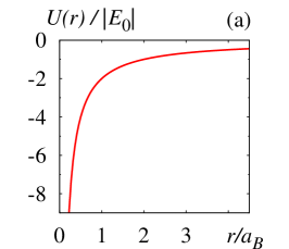
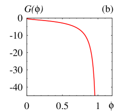
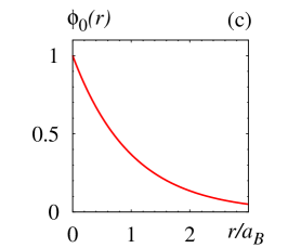
Figure 6: (a) The three-dimensional Coulomb potential in units of $|E_{0}|$ as function of $r$ in units of the Bohr radius $a_{B}$. (b) The nonlinear term $G(\phi)$ of the NSE defined in Eq. (47). (c) The radial part $\phi_{0}(r)$ of respectively the Coulomb ground state wave function or the soliton of the NSE (6) with the nonlinearity (47).

In Fig. 6, we depict for completeness the Coulomb potential $U(r)$, the nonlinear function $G(\phi)$, and the radial function $\phi_{0}(r)$. The function $G(\phi)$ is throughout negative for $\phi>0$ and diverges when $\phi\to 1$ which is in one-to-one correspondence to the divergence of the Coulomb potential at $r\to 0$.

XI Conclusions

In this work, we have presented a method to construct analytically solvable nonlinear extensions of the Schrödinger equation (NSE) starting from an ordinary analytically solvable Schrödinger equation (SE). We have illustrated the method through several examples in which the potential $U(\vec{x})$ of the SE in Eq. (1) was systematically transformed into a nonlinear term $F[\Psi^{\ast}\Psi]$ of the NSE in Eq. (6).

Starting from respectively the harmonic potential or (a special case) of the Rosen-Morse potential we rederived well-known soliton solutions of nonlinear theories, namely the Gausson in a general number of space dimensions $N$ and the one-dimensional 1/cosh soliton BialynickiBirula:1976zp ; BialynickiBirula:1979dp ; Oficjalski:1978 ; Zakharov-Shabat . In several other cases, we have derived exact soliton solutions of non-linear theories which, to the best of our knowledge, have not been discussed previously in literature. This includes among others a nonlinear theory derived from the SE with the Coulomb potential in $N=3$ dimensions. Another interesting example was a regular one-dimensional potential which can be transformed into the attractive $\delta(x)$ potential by taking one of the parameters of this potential to approach a specific limit. The regular potential as well as the singular $\delta(x)$ potential can both be used to construct exactly solvable NSE with interesting soliton solutions.

The quantum mechanical potentials explored in this work have in common that they are symmetric, i.e. $U(\vec{x})=U(r)$ with $r=|\vec{x}|$ in $N>1$ space dimensions or $U(x)=U(|x|)$ in $N=1$ space dimensions. Another common feature is that the considered potentials have a single minimum which can be finite or infinite. It is an interesting question whether the method can be generalized to construct exactly solvable nonlinear soliton theories also under more general conditions, e.g. starting from non-symmetric potentials or from double-well type potentials.

Another interesting future direction could be to explore systematically methods like Lie algebra techniques and self-similar potentials Shabat:1992 ; Spiridonov:1992 or the more general concept of shape invariant potentials Gendenshtein:1983skv and other supersymmetric methods in quantum mechanics Cooper:1994eh ; Bougie:2012 or whether novel soliton solutions can be found in non-hermitian PT symmetric quantum systems in analogous ways Ahmed:2001gz ; Musslimani:2008zz ; Konotop:2016eny . These interesting questions will be addressed in future studies.

Acknowledgments. This work was supported by the National Science Foundation under the Contract No. 1812423 and 2111490. This work was supported in part also by the Department of Energy within framework of the QGT Topical Collaboration

Appendix A Heisenberg’s uncertainty principle for extremely localized wave functions

In Sec. VII, we discussed the exactly solvable quantum potential (25). In this Appendix, we investigate in detail the limit $\lambda\to 0$ in which the ground state wave function (26) behaves such that the probability density has the properties

$$(i) \lim_{\lambda\to 0}|\Psi_{0}(t,x)|^{2}=0\quad\mbox{for}\quad x\neq 0\,,$$

$$(ii) \int\limits_{-\infty}^{\infty}\!\!dx\;|\Psi_{0}(t,x)|^{2}=1\quad\mbox{for}\quad\lambda\neq 0\,.$$ (48)

These properties imply that the probability density becomes extremely localized as

$$\lim_{\lambda\to 0}|\Psi_{0}(t,x)|^{2}=\delta(x),$$ (49)

and exhibits an obviously vanishing position uncertainty $\Delta x$. It is interesting to ask whether such an extremely localized state satisfies Heisenberg’s uncertainty principle. For $\lambda\neq 0$ it is always $\Delta p\;\Delta x>\frac{\hbar}{2}$. We refrain from showing the bulky analytic expressions for $\Delta p$ and $\Delta x$ which, if needed, can be found easily with mathematica and are given in terms of Gamma functions and hypergeometric functions. The results for $\Delta x$ and $\Delta p$ are shown in Fig. 7. As $\lambda$ decreases, the position uncertainty $\Delta x$ becomes smaller while the momentum uncertainty $\Delta p$ increases. For infinitesimally small (but non-zero) $\lambda$, the uncertainties behave as

$$\Delta x=a\sqrt{\frac{\lambda}{2}}+\dots\;,\quad\Delta p=\frac{\hbar}{a}\;\frac{1}{\sqrt{2\lambda}}+\dots\;,$$ (50)

where the dots indicate positive higher order corrections such that $\Delta x\,\Delta p>\frac{\hbar}{2}$ for all $\lambda>0$. The leading terms in Eq. (50) approximate the momentum and position uncertainties to within ${\cal O}(2\,\%)$ already for $\lambda\lesssim 10^{-1}$ and describe $\Delta p$ and $\Delta x$ over several orders of magnitude for $\lambda\ll 1$ in Fig. 7. From Eq. (49), we see that $\lim_{\lambda\to 0}\Delta p\;\Delta x=\frac{\hbar}{2}$. Thus, Heisenberg’s uncertainty relation is manifestly valid for any value of $\lambda$ including the limit $\lambda\to 0$.

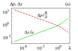
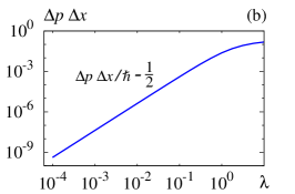
Figure 7: (a) Position uncertainty $\Delta x$ in units of $a$ and momentum uncertainty $\Delta p$ in units of $\hbar/a$ in the ground state (26) discussed in Sec. VII as functions of $\lambda$. The dotted lines show respectively the asymptotic results for $\Delta p$ and $\Delta x$ in Eq. (50). (b) Test of Heisenberg’s uncertainty relation expressed as $\Delta x\,\Delta p/\hbar-\frac{1}{2}$ which must be positive as is the case, see text.

The increasing of the momentum uncertainty $\Delta p$ as $\lambda$ becomes small implies a large kinetic energy. In fact, since in this stationary state $\langle p\rangle=0$, we have

$$\langle E_{\rm kin}\rangle=\frac{\langle p^{2}\rangle}{2m}=\frac{\Delta p^{2}}{2m}=\frac{\hbar^{2}}{2ma^{2}}\;\frac{1}{2\lambda}+\dots\;,$$ (51)

modulo subleading corrections for $\lambda\ll 1$. Thus, the expectation value of the kinetic energy diverges as $1/\lambda$ for $\lambda\to 0$ which is a consequence of the strong localization of the quantum state. However, it is important to keep in mind that the total (negative) binding energy $E_{0}$ is proportional to $1/\lambda^{2}$ in Eq. (26). Thus, when “measured in units” of the absolute value of the total energy, the expectation value of the kinetic energy actually behaves as

$$\frac{\langle E_{\rm kin}\rangle}{|E_{0}|}=\frac{\lambda}{2}+\dots\;$$ (52)

with the dots denoting higher order terms. In other words, $\langle E_{\rm kin}\rangle$ becomes negligibly small in the limit $\lambda\to 0$ in comparison to the total binding energy. This is because the ground state energy is dominated by the expectation value of the potential energy with the potential (25) behaving as $U(x)\propto 1/\lambda^{2}$. These properties make sense physically for arbitrarily small but non-zero values of $\lambda$. We deal with a deeply bound and strongly localized state. The fact that $\langle E_{\rm kin}\rangle\ll|E_{0}|$ means the motion of the particle becomes negligible as the particle becomes localized due to the strong coupling. Nevertheless, the uncertainty principle remains valid for any $\lambda$.

It is interesting to notice that the numerical computation of $\Delta p$ and $\Delta x$ can be carried out down to much smaller values of $\lambda$ than the numerical test of the uncertainty relation. The reason for that is as follows. At $\lambda=10^{-4}$ the asymptotic expressions in Eq. (50) underestimate $\Delta p$ in relative units by about ${\cal O}(2\times 10^{-5})$ and overestimate $\Delta x$ by about the same amount. We can go down to $\lambda=10^{-8}$ before hitting numerical accuracy limitations for $\Delta p$ and $\Delta x$ on the scale of Fig. 7a. However, the over- and underestimates in $\Delta p$ and $\Delta x$ largely compensate each other in the product such that at $\lambda=10^{-4}$ we reach with $\Delta p\,\Delta x/\hbar-\frac{1}{2}={\cal O}(4\times 10^{-10})$ our numerical accuracy in Fig. 7b.

The features that (i) ground state energy $E_{0}\to-\,\infty$ and (ii) probability density $|\psi_{0}(x,t)|^{2}\to\delta(x)$ occur also in the case of the attractive one-dimensional $1/|x|$-potential when the $1/|x|$ singularity is “regulated” as $1/(|x|+\epsilon)$ and the limit $\epsilon\to 0$ is taken Loudon:1959 . There is no deeper analogy between our case and the regularized $1/|x|$ potential. This is rather a generic feature of systems with strongly localized and deeply bound ground states. As long as the parameter ($\lambda$ in our case or $\epsilon$ in the regulated $1/|x|$ potential) is infinitesimally small but non-zero, one deals with a well-behaved quantum state. It has however been questioned whether the strict limit itself of such a strongly localized state with $|\psi_{0}(x,t)|^{2}\to\delta(x)$ constitutes a physical state, see Andrews:1966 .

References

- (1) M. Shifman, “Advanced topics in quantum field theory: A lecture course,” (Cambridge University Press, 2012), page 129. The quote refers to the critical magnetic monopole solution tHooft:1974kcl ; Polyakov:1974ek in the SU(2) Georgi-Manohar model Georgi:1972cj .
- (2) G. ’t Hooft, Nucl. Phys. B 79, 276-284 (1974).
- (3) A. M. Polyakov, Pisma Zh. Eksp. Teor. Fiz. 20, 430-433 (1974) [Engl. Translation JETP Lett. 20, 194-195 (1974)].
- (4) I. Białynicki-Birula and J. Mycielski, Annals Phys. 100 (1976) 62.
- (5) I. Białynicki-Birula and J. Mycielski, Phys. Scripta 20 (1979) 539-544.
- (6) B. A. Bechler and I. Białynicki-Birula, Acta Phys. Polon. 9, 759-775 (1978).
- (7) V. E. Zakharov and A. B. Shabat, Soviet Phys. JETP 34 62-69 (1972) [transl. of Zh. Eksp. Teor. Fiz. 61, 118-134 (1972)].
- (8) G. Rosen, Phys. Rev. 183, 1186-1188 (1969).
- (9) J. Hudson and P. Schweitzer, Phys. Rev. D 96, 114013 (2017) [arXiv:1712.05316 [hep-ph]].
- (10) E. Belendryasova, V. A. Gani and K. G. Zloshchastiev, Phys. Lett. B 823, 136776 (2021) [arXiv:2111.09096 [hep-th]].
- (11) E. P. Gross, Nuovo Cimento 20, 454 (1961).
- (12) L. P. Pitaevskii, Zh. Eksperim. i Teor. Fiz. 40, 646 (1961) [Soviet Phys. JETP 13, 451 (1961)].
- (13) Elliott H. Lieb and Werner Liniger, Phys. Rev. 130, 1605 (1963).
- (14) G. A. Askar’yan, Zh. Eksperim. i Teor. Fiz. 42, 1567 (1962) [translation: Soviet Phys. JETP 15, 1088 (1962)].
- (15) V. I. Talanov, Vysshikh Uchebn. Zavedenii, Radiofizika 7, 564 (1964) [translation: Radiophysics 7, 254 (1964)].
- (16) R. Y. Chiao, E. Garmire, and C. H. Townes, Phys. Rev. Lett. 13, 479 (1964); [Erratum Phys. Rev. Lett. 14, 1056 (1965)].
- (17) P. L. Kelley, Phys. Rev. Lett. 15, 1005 (1965) [Erratum Phys. Rev. Lett. 16, 384 (1966)].
- (18) T. Tsuzuki, J. Low Temp. Phys. 4, 441 (1971).
- (19) Vladimir V. Konotop and Lev Pitaevskii, Phys. Rev. Lett. 93, 240403 (2004).
- (20) T. Karpiuk, P. Deuar, P. Bienias, E. Witkowska, K. Pawłowski, M. Gajda, K. Rz ażewski, M. Brewczyk Phys. Rev. Lett. 109, 205302 (2012).
- (21) Yuri S. Kivshar and Barry Luther-Davies, Physics Reports 298, 81-197 (1998).
- (22) D. J. Frantzeskakis, J. Phys. A 43, 213001 (2010).
- (23) T. Yefsah, A. Sommer, M. Ku et al., Nature 499, 426-430 (2013).
- (24) D. H. Peregrine, Austral. Math. Soc. Ser. B 25, 16-43 (1983).
- (25) Christian Kharif and Efim Pelinovsky, European Journal of Mechanics B 22, 603-634 (2003).
- (26) L. Wang and Z. Yan, Appl. Math. Lett. 111, 106670 (2021) [arXiv:2012.09983 [nlin.PS]].
- (27) D. Solli, C. Ropers, P. Koonath, et al, Nature 450, 1054–1057 (2007).
- (28) A. H. Guth, M. P. Hertzberg and C. Prescod-Weinstein, Phys. Rev. D 92, 103513 (2015) [arXiv:1412.5930 [astro-ph.CO]].
- (29) M. Kormos, G. Mussardo, and A. Trombettoni, Phys. Rev. A 81, 043606 (2010).
- (30) M. A. B. Beg and R. C. Furlong, Phys. Rev. D 31, 1370 (1985)
- (31) M. H. Namjoo, A. H. Guth and D. I. Kaiser, Phys. Rev. D 98, 016011 (2018) [arXiv:1712.00445 [hep-ph]].
- (32) Michael I. Weinstein, Commun. Math. Phys. 87, 567-576 (1983).
- (33) O. Alvarez, L. A. Ferreira and J. Sanchez Guillen, Nucl. Phys. B 529, 689-736 (1998) [arXiv:hep-th/9710147 [hep-th]].
- (34) Vladimir N. Serkin and Akira Hasegawa, Phys. Rev. Lett. 85, 4502 (2000).
- (35) H. Blas and M. Zambrano, JHEP 03, 005 (2016) [arXiv:1511.04748 [hep-th]].
- (36) G. Biondini, D. K. Kraus and B. Prinari, Commun. Math. Phys. 348, 475-533 (2016) [arXiv:1511.02885 [nlin.SI]].
- (37) Rebekka Koch, Jean-Sébastien Caux, and Alvise Bastianello, J. Phys. A 55, 134001 (2022).
- (38) S. Weinberg, Phys. Rev. Lett. 62, 485 (1989); S. Weinberg, Annals Phys. 194, 336 (1989).
- (39) David E. Kaplan and Surjeet Rajendran, Phys. Rev. D 105, 055002 (2022).
- (40) C. G. Shull, D. K. Atwood, J. Arthur and M. A. Horne, Phys. Rev. Lett. 44, 765-768 (1980)
- (41) R. Gahler, A. G. Klein and A. Zeilinger, Phys. Rev. A 23, 1611-1617 (1981).
- (42) J. J. Bollinger, D. J. Heinzen, W. M. Itano, S. L. Gilbert and D. J. Wineland, Phys. Rev. Lett. 63, 1031-1034 (1989).
- (43) T. E. Chupp and R. J. Hoare, Phys. Rev. Lett. 64, 2261 (1990) [Erratum Phys. Rev. Lett. 66, 120 (1991)].
- (44) R. L. Walsworth, I. F. Silvera, E. M. Mattison and R. F. C. Vessot, Phys. Rev. Lett. 64, 2599-2602 (1990).
- (45) P. K. Majumder, B. J. Venema, S. K. Lamoreaux, B. R. Heckel and E. N. Fortson, Phys. Rev. Lett. 65, 2931-2934 (1990).
- (46) J. Broz, B. You, S. Khan, H. Haeffner, D. E. Kaplan and S. Rajendran, [arXiv:2206.12976 [quant-ph]].
- (47) N. Rosen and P. M. Morse, Phys. Rev. 42, 210 (1932).
- (48) G. A. Natanzon, Vestnik Leningrad Univ. 10, 22 (1971), Teoret. Mat. Fiz. 38, 146 (1979).
- (49) A. Shabat, Inverse Problems 8, 303 (1992).
- (50) V. Spiridonov, Phys. Rev. Lett. 69, 398 (1992).
- (51) L. E. Gendenshtein, JETP Lett. 38, 356-359 (1983)
- (52) F. Cooper, A. Khare and U. Sukhatme, Phys. Rept. 251, 267-385 (1995) [arXiv:hep-th/9405029 [hep-th]].
- (53) J. Bougie, A. Gangopadhyaya, J. Mallow, C. Rasinariu, Symmetry 4, 452-473 (2012).
- (54) Z. Ahmed, Phys. Lett. A 282, 343-348 (2001).
- (55) Z. H. Musslimani, K. G. Makris, R. El-Ganainy and D. N. Christodoulides, Phys. Rev. Lett. 100, 030402 (2008)
- (56) V. V. Konotop, J. Yang and D. A. Zezyulin, Rev. Mod. Phys. 88, no.3, 035002 (2016) [arXiv:1603.06826 [nlin.PS]].
- (57) R. Loudon, American Journal of Physics 27, 649 (1959).
- (58) M. Andrews, 1966 Am. J. Phys. 34, 1194-1195 (1966).
- (59) H. Georgi and S. L. Glashow, Phys. Rev. Lett. 28, 1494 (1972)