On large $3/2$-stable maps

Abstract

We discuss asymptotics of large Boltzmann random planar maps such that every vertex of degree $k$ has weight of order $k^{-2}$. Infinite maps of that kind were studied by Budd, Curien and Marzouk. These maps can be seen as the dual of the discrete $\alpha$-stable maps studied by Le Gall and Miermont for $\alpha=3/2$ or as the gaskets of critical $O(2)$-decorated random planar maps. We compute the asymptotics of the graph distance and of the first passage percolation distance between two uniform vertices, which are respectively equivalent in probability to $(\log\ell)^{2}/\pi^{2}$ and $2(\log\ell)/(\pi^{2}p_{\bf q})$ when the perimeter of the map $\ell$ goes to $\infty$, where $p_{\bf q}$ is a constant which depends on the model. We also show that the diameter is of the same order as those distances for both metrics and obtain in particular that these maps do not satisfy scaling limits in the sense of Gromov-Prokhorov or Gromov-Hausdorff for lack of tightness. To study the peeling exploration of these maps, we prove local limit and scaling limit theorems for a class of random walks with heavy tails conditioned to remain positive until they die at $-\ell$ towards processes that we call stable Lévy processes conditioned to stay positive until they jump and die at $-1$.

Figure 1: Simulation of a $3/2$-stable map $\mathfrak{M}^{(500,\dagger)}$ of perimeter $1000$. The two large red spheres are two uniform random vertices of $\mathfrak{M}^{(500,\dagger)}$ and the red path is the shortest path between them.

1 Introduction

1.1 Boltzmann $3/2$-stable planar maps

Random planar maps have been studied very actively, motivated partly by their connections with two dimensional Liouville quantum gravity. In this work, we study the geometry of large random $3/2$-stable Boltzmann planar maps. A planar map $\mathfrak{m}$ is a planar graph embedded in the sphere seen up to orientation-preserving homeomorphism and equipped with a distinguished oriented edge $\vec{e}_{r}$ called the root edge. The face $f_{r}$ adjacent to the right of the root edge is called the root face. The degree of $f_{r}$ is also called the perimeter of $\mathfrak{m}$. We also require the map $\mathfrak{m}$ to be bipartite, i.e. that all its faces have even degree, inasmuch as the enumeration of bipartite maps is particularly simple. We write $\mathcal{M}$ for the set of finite bipartite rooted planar maps.

Random planar maps can be picked uniformly at random among maps of a given size. A more general way to pick a random map $\mathfrak{m}\in\mathcal{M}$ is to assign Boltzmann weights to them, following [22]. Let ${\bf q}=(q_{k})_{k\geq 1}$ be a non-zero sequence of non-negative numbers called the sequence of weights. The weight of a map $\mathfrak{m}\in\mathcal{M}$ is defined as

$$w_{\bf q}(\mathfrak{m})=\prod_{f\in\mathrm{Faces}(\mathfrak{m})\setminus\left\{f_{r}\right\}}q_{\mathrm{deg}(f)/2}.$$

For all $\ell\geq 1$, let $\mathcal{M}^{(\ell)}\subset\mathcal{M}$ be the set of all (finite) maps with perimeter $2\ell$. We introduce the partition function

$$W^{(\ell)}=\sum_{\mathfrak{m}\in\mathcal{M}^{(\ell)}}w_{\bf q}(\mathfrak{m}).$$

When $W^{(1)}<\infty$, we say that $\bf q$ is admissible. In what follows, we also require the weight sequence to be critical of type $a\in(3/2,5/2]$, which is equivalent by Proposition 5.10 of [13] to having

$$W^{(\ell)}\mathop{\sim}\limits_{\ell\to\infty}\frac{p_{\bf q}}{2}c_{\bf q}^{\ell+1}\ell^{-a},$$ (1.1)

for some constant $p_{\bf q}>0$. The cases $a\in(3/2,5/2)$ are called non-generic. Such sequences $\bf q$ do exist, see Lemma 6.1 of [10] for explicit examples. If $\bf q$ is admissible, we write $\mathbb{P}^{(\ell)}$ the probability measure on $\mathcal{M}^{(\ell)}$ associated to the weight sequence ${\bf q}$, called the Boltzmann measure, defined by

$$\mathbb{P}^{(\ell)}(\mathfrak{m})=\frac{w_{\bf q}(\mathfrak{m})}{W^{(\ell)}}.$$

We also write $\mathbb{E}^{(\ell)}$ for the associated mathematical expectation. A random map $\mathfrak{M}^{(\ell)}$ following the law $\mathbb{P}^{(\ell)}$ is called a $\bf q$-Boltzmann random map of perimeter $2\ell$. The $\bf q$-Boltzmann random maps for $\bf q$ of type $a$ are also called $(a-1/2)$-stable maps. The object of study in this work is not the map $\mathfrak{M}^{(\ell)}$ in itself but rather its dual map $\mathfrak{M}^{(\ell,\dagger)}$ obtained by exchanging the roles of the faces and of the vertices.

For $a=2$, the local limit, the infinite $3/2$-stable map, was studied in [11] by Budd, Curien and Marzouk. In particular, they established the scaling limit of the perimeter associated to the exploration of the infinite map, and studied its basic metric properties and their results will be especially helpful in Section 4.

The peeling exploration of the map makes appear a random walk $S$ on $\mathbb{Z}$ with step distribution $\nu$ which will play a crucial part in this work. It is related to $\bf q$ by

$$\forall k\geq 0,\enskip\nu(k)=q_{k+1}c_{\bf q}^{k}\qquad\text{and}\qquad\nu(-k-1)=2W^{(k)}c_{\bf q}^{-k-1}.$$ (1.2)

When $\bf q$ is critical of type $a=2$, we know in particular by Proposition 5.10 of [13] that

$$\nu(-k)\sim p_{\bf q}k^{-2}\qquad\text{and}\qquad\nu([k,\infty))\sim p_{\bf q}k^{-1}\enskip\text{ as }k\longrightarrow\infty,$$ (1.3)

so that $\nu$ is in the domain of attraction of the symmetric Cauchy process (with no drift).

1.2 Main results

Throughout this work, unless explicitly stated otherwise, $\bf q$ will be a critical non-generic weight sequence of type $a=2$ and, for all $\ell\geq 1$, $\mathfrak{M}^{(\ell)}$ will be a $\bf q$-Boltzmann random map of perimeter $2\ell$.

Before stating the main results, let us introduce the distance functions on a map $\mathfrak{m}$. For every faces $f_{1}$, $f_{2}$ of $\mathfrak{m}$, we denote by $d_{\mathrm{gr}}^{\dagger}(f_{1},f_{2})$ the graph distance between $f_{1}$ and $f_{2}$ in the dual map $\mathfrak{m}^{\dagger}$. Another distance, easier to study in our context, is the first-passage percolation distance $d_{\mathrm{fpp}}^{\dagger}$ defined as follows: to each edge of $\mathfrak{m}^{\dagger}$ we assign an independent random variable following the exponential law of parameter $1$ (that we will write $\mathcal{E}(1)$), interpreted as its random length. For every faces $f_{1}$, $f_{2}$ of $\mathfrak{m}$, we then denote by $d_{\mathrm{fpp}}^{\dagger}(f_{1},f_{2})$ the distance between $f_{1}$ and $f_{2}$ in the dual map $\mathfrak{m}^{\dagger}$ whose edges are equipped with those random lengths.

The first theorem describes the distance from the root face to a uniform random face (we also prove that the same results hold for a uniform random edge or a uniform random vertex).

Theorem 1.1.

For all $\ell\geq 1$, let $F^{(\ell)}$ be a random uniform face in $\mathfrak{M}^{(\ell)}$ (conditionally on $\mathfrak{M}^{(\ell)}$) and recall that $f_{r}$ is the root face. Then

$$\frac{d_{\mathrm{fpp}}^{\dagger}(f_{r},F^{(\ell)})}{\log\ell}\mathop{\longrightarrow}\limits_{\ell\to\infty}^{(\mathbb{P})}\frac{1}{\pi^{2}p_{\bf q}}\qquad\text{and}\qquad\frac{d_{\mathrm{gr}}^{\dagger}(f_{r},F^{(\ell)})}{(\log\ell)^{2}}\mathop{\longrightarrow}\limits_{\ell\to\infty}^{(\mathbb{P})}\frac{1}{2\pi^{2}}.$$

The scales for the distances in $\log\ell$ and $(\log\ell)^{2}$ are specific to the $3/2$-stable case on account of its criticality and of the singular behavior of Cauchy processes. Deeply related behaviors have already been observed for the volume growth of balls in the infinite map in Theorems A and B of [11].

We then prove that the geodesics from the root to two uniform random faces “split very quickly”, so that we get the asymptotic of the distance between two uniform random faces, see Corollary 5.1. This corollary implies that if $(F_{i}^{(\ell)})_{i\geq 1}$ are i.i.d. uniform random faces of $\mathfrak{M}^{(\ell)}$ for all $\ell\geq 1$, then for the product topology,

$$\left(\frac{d_{\mathrm{fpp}}^{\dagger}(F_{i},F_{j})}{\log\ell}\right)_{i,j\geq 1}\mathop{\longrightarrow}\limits_{\ell\to\infty}^{(\mathbb{P})}\left(\frac{2}{\pi^{2}p_{\bf q}}\right)_{i,j\geq 1}\qquad\text{and}\qquad\left(\frac{d_{\mathrm{gr}}^{\dagger}(F_{i},F_{j})}{(\log\ell)^{2}}\right)_{i,j\geq 1}\mathop{\longrightarrow}\limits_{\ell\to\infty}^{(\mathbb{P})}\left(\frac{1}{\pi^{2}}\right)_{i,j\geq 1}.$$ (1.4)

So as to study the diameter in Section 6, we control the distances uniformly on all the faces. Aside from the first and second moment methods, a convenient tool is a martingale associated to the perimeter process, hence enabling us to show that the diameter is of the same order as the distance between two faces picked uniformly at random.

Theorem 1.2.

Let $\mathrm{Diam}_{\mathrm{gr}}^{\dagger}(\mathfrak{M}^{(\ell)})$ (resp. $\mathrm{Diam}_{\mathrm{fpp}}^{\dagger}(\mathfrak{M}^{(\ell)})$) be the diameter of $\mathfrak{M}^{(\ell,\dagger)}$ for the graph distance (resp. fpp distance). Let $\delta>0$. There exists a constant $K({\bf q})$ depending on $\bf q$ such that, with probability $1-o(1)$ when $\ell\to\infty$,

$$\left(\frac{3}{4(1-q_{1}^{2})}\vee\frac{2}{\pi^{2}p_{\bf q}}\right)-\delta\leq\frac{\mathrm{Diam}_{\mathrm{fpp}}^{\dagger}(\mathfrak{M}^{(\ell)})}{\log\ell}\leq K({\bf q})\qquad\text{and}\qquad\frac{1}{\pi^{2}}-\delta\leq\frac{\mathrm{Diam}_{\mathrm{gr}}^{\dagger}(\mathfrak{M}^{(\ell)})}{(\log\ell)^{2}}\leq 18+\delta.$$

These bounds on the diameter indicate in particular the scale at which one should look for studying Gromov-Hausdorff convergence. Actually, (1.4) shows that at the macroscopic scale, $\mathfrak{M}^{(\ell),\dagger}$ looks like a star with many branches when $\ell\to\infty$, see the simulation in Figure 1. As a consequence, the sequence $\left(\mathfrak{M}^{(\ell),\dagger}\right)_{\ell\geq 1}$ equipped with the rescaled distances is not tight, neither for the Gromov-Hausdorff topology, nor for the Gromov-Prokhorov topology. Indeed, one the one hand, the limit of any subsequence can not be compact due to (1.4), while on the other hand any limiting random separable metric measured space $(X,d,\mu)$ of some subsequence for Gromov-Prokhorov would have an empty support since two uniform points of law $\mu$ would be at constant distance by (1.4), which contradicts the separability (see e.g. Remark 4.5 of [17] for details on this reasoning).

More precisely, for all $\ell\geq 1$, let $\mu_{\ell}$ be the uniform measure on the faces of $\mathfrak{M}^{(\ell)}$. We have thus shown the following corollary.

Corollary 1.3.

The sequences $(\mathfrak{M}^{(\ell,\dagger)},\frac{1}{(\log\ell)^{2}}d_{\mathrm{gr}}^{\dagger},\mu_{\ell})_{\ell\geq 1}$ and $(\mathfrak{M}^{(\ell,\dagger)},\frac{1}{\log\ell}d_{\mathrm{fpp}}^{\dagger},\mu_{\ell})_{\ell\geq 1}$ are not tight for the Gromov-Prokhorov topology. Besides, the sequences $(\mathfrak{M}^{(\ell,\dagger)},\frac{1}{(\log\ell)^{2}}d_{\mathrm{gr}}^{\dagger})_{\ell\geq 1}$ and $(\mathfrak{M}^{(\ell,\dagger)},\frac{1}{\log\ell}d_{\mathrm{fpp}}^{\dagger})_{\ell\geq 1}$ are not tight for the Gromov-Hausdorff topology. In particular, there is no Gromov-Hausdorff scaling limit of any subsequence of $(\mathfrak{M}^{(\ell,\dagger)},d_{\mathrm{gr}}^{\dagger})_{\ell\geq 1}$ or $(\mathfrak{M}^{(\ell,\dagger)},d_{\mathrm{fpp}}^{\dagger})_{\ell\geq 1}$

Still, following [16] and [18], the convergence $(\ref{eq étoile})$ can also be interpreted as the convergence in probability of $(\mathfrak{M}^{(\ell,\dagger)},\frac{1}{(\log\ell)^{2}}d_{\mathrm{gr}}^{\dagger},\mu_{\ell})_{\ell\geq 1}$ and $(\mathfrak{M}^{(\ell,\dagger)},\frac{1}{\log\ell}d_{\mathrm{fpp}}^{\dagger},\mu_{\ell})_{\ell\geq 1}$ towards some long dendrons defined in Example 7.2 of [18].

1.3 Conditioned random walks

The main technique to study the metric properties of $\mathfrak{M}^{(\ell,\dagger)}$ is the filled-in peeling exploration. It was first introduced in [27] and [1] for triangulations. A general version is defined in [8] and is presented in Section 3. See [7] and [13] for a more detailed introduction. The peeling process consists in a step-by-step Markovian exploration of the map starting from the root face according some peeling algorithm. At each step, the peeling process reveals the face behind the peeled edge chosen by the peeling algorithm. Various choices of peeling algorithms enable to understand different properties of the map. Our use of the peeling algorithm is similar to that of [10] for the study of infinite $(a-1/2)$-stable Boltzmann maps for $\bf q$ critical non-generic of type $a\in(3/2,5/2)\setminus\left\{2\right\}$ and [11] for the study of infinite $3/2$-stable Boltzmann maps. A difference is that most of the time we will work with the peeling algorithm on the map which has been rerooted (see Subsection 3.4).

In our case, the evolution of the perimeter of the explored part has the same law as the $\nu$-random walk conditioned to stay positive until it jumps and dies at $-\ell$. This is, to the best of our knowledge, a new type of conditioning which we study in details in Section 2. In that section we introduce a key coupling (Lemma 2.5) between this conditioned random walk and the $\nu$-random walk conditioned to stay positive forever, using that such conditionings can be performed via Doob $h$-transforms. This coupling enables us in particular to use some results of [11]. This lemma states that for all $n\geq 1$, there exists a coupling between the two conditioned random walks such that if the second one has not been killed yet at time $n$, then the two conditioned random walks coincide.

The rest of Section 2 can be seen as an asymptotic study of this conditioned $\nu$-random walk. We first prove a local limit theorem for the lifetime and the last positive value of the walk. Relying on this local limit, we next establish in Theorem 2.8 the scaling limit of that conditioned random walk dying at $-\ell$ towards a process that we call an $(a-1)$-stable Lévy process conditioned to die at $-1$. We hope that those results could be fruitful in other contexts.

1.4 Discussion

The gasket of a critical $O(n)$ loop-decorated planar map, which is obtained after deleting the edges and vertices in the outermost loops, is a particular example of an $(a-1/2)$-stable map, where the case $n=2$ corresponds to $a=2$. This relation is depicted for instance in [21, 5]. The $O(n)$ loop-decorated maps undergo a phase transition described in [5, 9]. The critical case $n=2$ is often excluded in the literature. For the infinite Boltzmann $(a-1/2)$-stable maps, in [10] a phase transition at $a=2$ is equally exhibited. Let us also mention the conjecture that for $n=2$ the gasket should converge in some sense to the $\mathrm{CLE}_{4}$ ensemble (introduced in [23, 24]).

We are confident that some of our results such as Theorem 1.1 and Corollary 5.1 can be extended to the case $a\in(3/2,2)$ with a $\log\ell$ scaling for the dual graph distance. The martingale (6.1) seems also adapted in this setting, so that Theorem 1.2 should have an analog in this case.

2 The random walk conditioned to die at $-\ell$

This section is devoted to the study the $\nu$-random walk $S$ conditioned to stay positive until it jumps and dies at $-\ell$, which will be denoted by $(P_{\ell}(n))_{n\geq 0}$ under $\mathbb{P}_{\ell}^{(1)}$. We establish in Lemma 2.5 a coupling between this conditioned random walk and the random walk conditioned to stay always positive. We then prove a local limit result for the hitting time $\tau_{-\ell}$ of $-\ell$ (Proposition 2.7) which we use to establish a scaling limit (Theorem 2.8).

2.1 The $\nu$ random walk, harmonic functions and conditionings

The criticality condition (1.1) imposes strong properties on the step distribution $\nu$ which are better stated in terms of harmonic functions. For all $\ell\geq 0$ and $p\geq 1$, let

$$h^{\downarrow}_{p}(\ell)=h^{\downarrow}(\ell)h^{\downarrow}(p)\frac{\ell}{\ell+p}\qquad\text{and}\qquad h_{0}^{\downarrow}(\ell)=h^{\downarrow}(\ell)=2^{-2\ell}\binom{2\ell}{\ell},$$ (2.1)

with by convention $h^{\downarrow}(\ell)=h_{p}^{\downarrow}(\ell)=0$ for $\ell<0$ except for $\ell=p$ where we set $h_{p}(-p)=1$. We also set $h^{\uparrow}(\ell)=2\ell h^{\downarrow}(\ell)$ for all $\ell\in\mathbb{Z}$. Let $a\in(3/2,5/2]$. In the rest of this section we only assume that $\nu$ is a probability measure on $\mathbb{Z}$ such that

1. The functions $h^{\downarrow}$ and $h^{\uparrow}$ are harmonic for $\nu$.

2. We have $\nu(-k)\sim p_{\bf q}/k^{a}$ as $k\to\infty$.

These two conditions are equivalent to the criticality of type $a$ of the weight sequence $\bf q$ associated to $\nu$ by (1.2) (see the paragraph 3.2 in [8], Theorem 1 and Proposition 5 of [7] or Theorem 5.4 and its proof in [13] for (I), and Propositions 5.9 and 5.10 of [13] for (II)). The admissibility of $\bf q$ then entails the harmonicity of $h^{\downarrow}_{p}$ for $S$ for all $p\geq 1$ (see the proof of Lemma 5.2 in [13]).

It is also known (see e.g. Proposition 10.1 in [13]) that $(S_{\lfloor nt\rfloor}/n^{1/(a-1)})_{t\geq 0}$ converges in distribution towards $p_{\bf q}^{1/(a-1)}\Upsilon_{a}$ for the Skorokhod topology, where $\Upsilon_{a}$ is the $(a-1)$-stable Lévy process starting at zero with positivity parameter $\rho=\mathbb{P}(S_{t}\geq 0)$ satisfying $(a-1)(1-\rho)=1/2$, normalized so that its Lévy measure is $\cos(a\pi)(dx/x^{a}){\bf 1}_{x>0}+(dx/|x|^{a}){\bf 1}_{x<0}$.

Finally, from the harmonic functions, one can define the corresponding Doob $h$-transforms of the $\nu$ random walk $S$. For all $\ell\geq 1$, we denote by $(P_{\infty}(n))_{n\geq 0}$ under $\mathbb{P}^{(\ell)}_{\infty}$ the Doob $h^{\uparrow}$-transform of $S$ starting at $\ell$ and for all $\ell\geq 1,p\geq 0$, we write $(P_{p}(n))_{n\geq 0}$ under $\mathbb{P}^{(\ell)}_{p}$ the Doob $h^{\downarrow}_{p}$-transform of $S$ killed when it reaches $-p$. The notation is chosen to be consistent with the rest of the paper since these conditioned random walks will be the perimeter processes in Section 3. The Doob $h^{\uparrow}$-transform of $S$ can be seen as the random walk $S$ conditioned to stay always positive while the Doob $h^{\downarrow}_{p}$-transform of $S$ killed at $-p$ can be understood analogously as the random walk conditioned to stay positive until it is killed at $-p$ (see [13] Proposition 5.3).

2.2 Preliminaries on the random walk conditioned to stay positive

Before delving into the study of the walk $P_{\ell}$ under $\mathbb{P}^{(1)}_{\ell}$, we record for future use some known results on the walks $P_{\infty}$, $P_{p}$ under $\mathbb{P}^{(1)}_{\infty}$, $\mathbb{P}^{(\ell)}_{p}$ for fixed $p$ as $\ell\to+\infty$. One of the most useful results will be the scaling limit of the random walk conditioned to stay always positive $P_{\infty}$ under $\mathbb{P}^{(1)}_{\infty}$. This scaling limit was introduced in [10] and [11] using Theorem 1.1 from [12]. The limit is described informally as the Lévy process $\Upsilon_{a}$, introduced in the above subsection, conditioned to stay positive and starting from zero. To do this, one can first define the process $(\mathcal{S}^{\uparrow}_{x}(t))_{t\geq 0}$ starting at some $x>0$ as the Doob $h$-transform of $(x+\Upsilon_{a}(t))_{t\geq 0}$ starting at $x$, using the harmonic function $h:y\mapsto{\bf 1}_{y\geq 0}\sqrt{y}$. The process $(\mathcal{S}^{\uparrow}_{x}(t))_{t\geq 0}$ then converges in distribution when $x\to 0$ towards a process written $\Upsilon_{a}^{\uparrow}$ which starts at zero. Recall the constant $p_{\bf q}$ which first appears in (1.1).

Theorem 2.1.

(Proposition 10.3 of [13]) The following convergence holds for the $J_{1}$-Skorokhod topology: under $\mathbb{P}^{(1)}_{\infty}$,

$$\left(\frac{P_{\infty}(\lfloor nt\rfloor)}{n^{1/(a-1)}}\right)_{t\geq 0}\enskip\mathop{\longrightarrow}\limits_{n\to\infty}^{(\mathrm{d})}\enskip\left(\Upsilon_{a}^{\uparrow}(p_{\bf q}t)\right)_{t\geq 0}\mathop{=}\limits^{(\mathrm{d})}\left(p_{\bf q}^{1/(a-1)}\Upsilon_{a}^{\uparrow}(t)\right)_{t\geq 0}.$$

The proof of Theorem 1.1 in [12] relies mostly on the scaling limit of the $\nu$-random walk $S$ conditioned to stay positive until some time towards a stable meander: let $\widetilde{\Upsilon}_{a}$ be the meander of length $1$ associated to $\Upsilon_{a}$, which is informally the process $\Upsilon_{a}$ conditioned to remain positive up to time $1$. Then the following theorem is a consequence of the main theorem of [14].

Theorem 2.2.

([14]) For $S_{0}=1$, conditionnally on $S_{1},\ldots,S_{n}>0$, the process $(S(\lfloor nt\rfloor)/n^{1/(a-1)})_{t\geq 0}$ converges in distribution for the $J_{1}$-Skorokhod topology towards $(p_{\bf q}^{1/(a-1)}\widetilde{\Upsilon}_{a}(t))_{t\geq 0}$.

The density of $\Upsilon_{a}^{\uparrow}(1)$ (resp. $\widetilde{\Upsilon}_{a}(1)$) will be written $f^{\uparrow}_{a}$ (resp. $\tilde{f}_{a}$). We know from [15] that $\tilde{f}_{a}$ is continuous and bounded (and also bounded away from zero on any compact of $(0,\infty)$) and moreover that there exists $C_{1}>0$ such that $f_{a}^{\uparrow}(x)=C_{1}x^{1/2}\tilde{f}_{a}(x)$.

Besides, so as to establish our local limit results, we state the following lemma which is an extension and a reformulation of Lemma 3 (i) of [11]. Its proof is exactly the same as in [11] and builds upon [26].

Lemma 2.3.

(Lemma 3 (i) from [11]) Uniformly on $x\geq 1$ as $n\to\infty$,

$$\mathbb{P}_{1}\left(S_{1},\ldots,S_{n}\geq 1\text{ and }S_{n}=x\right)\enskip=\enskip\frac{\sqrt{\pi}}{2(np_{\bf q})^{1/(a-1)}\sqrt{x}}f_{a}^{\uparrow}\left(\frac{x}{(p_{\bf q}n)^{1/(a-1)}}\right)+o(n^{-3/(2(a-1))}).$$

Finally, the next proposition, which describes the scaling limit of $P_{p}$ under $\mathbb{P}^{(\ell)}_{p}$ for fixed $p$, will be of some use in Section 5. The scaling limit is described by the Lévy process $\Upsilon_{a}^{\downarrow}$ conditioned to stay positive until it dies continuously at zero. The process $\Upsilon_{a}^{\downarrow}$ can be defined as a Doob transform of $\Upsilon_{a}+1$ using the harmonic function $x\mapsto(1/\sqrt{x}){\bf 1}_{x>0}$. This proposition slightly extends a particular case of Proposition 6.6 from [2]. Not only does its proof rely on the convergence in distribution of $(S_{\lfloor nt\rfloor}/n^{1/(a-1)})_{t\geq 0}$ towards $p_{\bf q}^{1/(a-1)}\Upsilon_{a}$ but it also relies on Theorem 1.3 of [12] in the case $p=0$. In that case $P_{0}$ is a Doob $h^{\downarrow}$ transform of the $\nu$-random walk, i.e. a random walk conditioned to die at zero. The proof of Theorem 1.3 in [12] can be rewritten by replacing $h^{\downarrow}$ (which is denoted by $W$ in [12]) by $h^{\downarrow}_{p}$, i.e. by replacing the walk conditioned to die at zero by a walk conditioned to stay positive until it dies at $-p$.

Proposition 2.4.

(Extension of Proposition 6.6 from [2]) For all $p\geq 0$, the following convergence holds for the $J_{1}$-Skorokhod topology: under $\mathbb{P}^{(\ell)}_{p}$,

$$\left(\frac{P_{p}(\lfloor\ell^{a-1}t\rfloor)}{\ell}\right)_{t\geq 0}\enskip\mathop{\longrightarrow}\limits_{\ell\to\infty}^{(\mathrm{d})}\enskip\left(\Upsilon_{a}^{\downarrow}(p_{\bf q}t)\right)_{t\geq 0}.$$

Moreover, jointly with the above convergence, we have the convergence of the lifetimes:

$$\frac{\tau_{-p}}{\ell^{a-1}}\enskip\mathop{\longrightarrow}\limits_{\ell\to\infty}^{(\mathrm{d})}\enskip\frac{\zeta}{p_{\bf q}},$$

where $\tau_{-p}=\inf\left\{n\geq 0;\ P_{p}(n)=-p\right\}$ and $\zeta=\inf\left\{t\geq 0;\ \Upsilon_{a}^{\downarrow}(t)=0\right\}$.

One may alternatively prove the first convergence of the above proposition by applying Theorem 2 of [3] while the second assertion can be seen as a consequence of Theorem 3 (i) of [3].

2.3 Coupling random walks conditioned to stay positive with random walks conditioned to die at $-\ell$

Let us denote by $\tau_{-\ell}$ the first hitting time of $-\ell$ by $(P_{\ell}(k))_{k\geq 0}$ the random walk conditioned to remain positive until it dies at $-\ell$ under $\mathbb{P}^{(1)}_{\ell}$. Let us first state a coupling lemma which will be useful in this section and in the next ones. In particular, it will enable us to take advantage of the results from [11] in Section 4.

Lemma 2.5.

There exists a coupling of the random walks $P_{\ell}$ under $\mathbb{P}^{(1)}_{\ell}$ and $P_{\infty}$ under $\mathbb{P}^{(1)}_{\infty}$ up to time $n$ written $\mathbb{P}^{(1),n}_{\ell,\infty}$ such that: under $\mathbb{P}^{(1),n}_{\ell,\infty}$, for all $s_{1},\ldots,s_{n}\in\mathbb{N}^{*}$, conditionally on $(P_{\infty}(k))_{1\leq k\leq n}=(s_{k})_{1\leq k\leq n}$, the equality $(P_{\ell}(k))_{1\leq k\leq n}=(s_{k})_{1\leq k\leq n}$ holds with probability $\frac{1+\ell}{s_{n}+\ell}$ and $\tau_{-\ell}\leq n$ with probability $1-\frac{1+\ell}{s_{n}+\ell}$ (see Figure 2).

Figure 2: Simulation of the conditioned random walks $P_{\infty}$ and $P_{\ell}$ under the coupling $\mathbb{P}^{(1),n}_{\ell,\infty}$ in the case $\tau_{-\ell}>n$ for $n=1000$ and $\ell=2000$ (after time $n$, we let both processes evolve independently).

Proof.

The key ingredient of the proof is the relation $h^{\downarrow}_{\ell}(k)=h^{\downarrow}(\ell)h^{\uparrow}(k)/(2(\ell+k))$ for $k,\ell\geq 1$ coming from the exact expression of the harmonic functions. From the definition of $P_{\ell}$ under $\mathbb{P}^{(1)}_{\ell}$ as a $h^{\downarrow}_{\ell}$-Doob transform of a $\nu$-random walk $S$, we note that if $s_{1},\ldots,s_{n}\in\mathbb{N}^{*}$, then

$$\mathbb{P}^{(1)}_{\ell}((P_{\ell}(k))_{1\leq k\leq n}=(s_{k})_{1\leq k\leq n}) =\frac{h^{\downarrow}_{\ell}(s_{n})}{h^{\downarrow}_{\ell}(1)}\mathbb{P}_{1}((S_{k})_{1\leq k\leq n}=(s_{k})_{1\leq k\leq n})$$

$$=\frac{h^{\uparrow}(s_{n})}{h^{\uparrow}(1)}\frac{1+\ell}{s_{n}+\ell}\mathbb{P}_{1}((S_{k})_{1\leq k\leq n}=(s_{k})_{1\leq k\leq n})$$

$$=\frac{1+\ell}{s_{n}+\ell}\mathbb{P}^{(1)}_{\infty}((P_{\infty}(k))_{1\leq k\leq n}=(s_{k})_{1\leq k\leq n})$$

$$\leq\mathbb{P}^{(1)}_{\infty}((P_{\infty}(k))_{1\leq k\leq n}=(s_{k})_{1\leq k\leq n}).$$

One can thus define such a coupling. ∎

One can see from the proof that the above lemma only relies on condition (I). A simple consequence of this coupling is a limit theorem for $\tau_{-\ell}/\ell^{(a-1)}$ when $\bf q$ has type $a\in(3/2,5/2]$. Recall that $\Upsilon_{a}^{\uparrow}$ is the stable Lévy process $\Upsilon_{a}$ starting at zero conditioned to stay positive.

Proposition 2.6.

We have the convergence in law ${\tau_{-\ell}}/{\ell^{a-1}}\mathop{\longrightarrow}\limits_{\ell\to\infty}^{\text{d}}\tilde{\tau}/p_{\bf q}$ where $\tilde{\tau}$ is a random variable such that for all $u\geq 0$, $\mathbb{P}(\tilde{\tau}\geq u)=\mathbb{E}({1/(1+\Upsilon_{a}^{\uparrow}(u))}).$

Proof.

By Lemma 2.5 and Theorem 2.1, for every $u\geq 0$,

$$\mathbb{P}^{(1)}_{\ell}(\tau_{-\ell}>u\ell^{a-1}) =\mathbb{E}^{(1)}_{\infty}\frac{1+\ell}{P_{\infty}({\lfloor u\ell^{a-1}\rfloor})+\ell}\mathop{\longrightarrow}\limits_{\ell\to\infty}\mathbb{E}\frac{1}{1+\Upsilon_{a}^{\uparrow}(p_{\bf q}u)},$$

and the claim follows. ∎

2.4 Local limit results for the random walk conditioned to die at $-\ell$

The result of Proposition 2.6 can be refined to obtain a joint local limit theorem for the lifetime $\tau_{-\ell}$ together with the last positive value of the conditioned random walk $P_{\ell}(\tau_{-\ell}-1)$:

Proposition 2.7.

For all $\varepsilon>0$ the convergence below holds uniformly in $u,s\in[\varepsilon,\varepsilon^{-1}]$:

$$\ell^{a}\mathbb{P}^{(1)}_{\ell}(\tau_{-\ell}=\lfloor\ell^{a-1}s\rfloor\text{ and }P_{\ell}(\tau_{-\ell}-1)=\lfloor\ell u\rfloor)\mathop{\longrightarrow}\limits_{\ell\to\infty}\frac{\pi p_{\bf q}^{1-1/(a-1)}}{s^{1/(a-1)}}\frac{1}{\sqrt{u}(1+u)^{a}}f_{a}^{\uparrow}\left(\frac{u}{(p_{\bf q}s)^{1/(a-1)}}\right),$$

and the right-hand side is a probability density.

Proof.

Let $\varepsilon>0$. Let us write $n=\lfloor\ell^{a-1}s\rfloor$ and $x=\lfloor\ell u\rfloor$. Then,

$$\frac{1}{2}\frac{h^{\downarrow}(\ell)}{\ell+1}\mathbb{P}^{(1)}_{\ell}(\tau_{-\ell}=\lfloor\ell^{a-1}s\rfloor\text{ and }P_{\ell}(\tau_{-\ell}-1)=\lfloor\ell u\rfloor)=\mathbb{P}_{1}(S_{1},\ldots,S_{n-1}\geq 1\text{ and }S_{n-1}=x)\nu(-\ell-x).$$

But by Lemma 2.3 and since $\nu(-k)\sim p_{\bf q}k^{-a}$ as $k\to\infty$ by (II), uniformly in $u,s\in[\varepsilon,\varepsilon^{-1}]$,

$$\mathbb{P}_{1}(S_{1},\ldots,S_{n-1}\geq 1\text{ and }S_{n-1}=x)\nu(-\ell-x) \mathop{\sim}\limits_{\ell\to\infty}\frac{\sqrt{\pi}p_{\bf q}^{1-1/(a-1)}}{2s^{1/(a-1)}\ell^{a+3/2}}f_{a}^{\uparrow}\left({u\over(p_{\bf q}s)^{1/(a-1)}}\right)\frac{1}{\sqrt{u}(1+u)^{a}}.$$

This proves the desired convergence using that $h^{\downarrow}(\ell)\sim 1/\sqrt{\pi\ell}$ as $\ell\to\infty$. Let us check that the right term indeed corresponds to a probability density, in other words that

$$\int_{0}^{\infty}\frac{\pi p_{\bf q}^{1-1/(a-1)}}{s^{1/(a-1)}}\int_{0}^{\infty}f_{a}^{\uparrow}\left(\frac{u}{(p_{\bf q}s)^{1/(a-1)}}\right)\frac{1}{\sqrt{u}(1+u)^{a}}duds=1$$

By the change of variable $w=\frac{u}{(p_{\bf q}s)^{1/(a-1)}}$ at fixed $u$,

$$\int_{0}^{\infty}\frac{\pi p_{\bf q}^{1-1/(a-1)}}{s^{1/(a-1)}}\int_{0}^{\infty}f_{a}^{\uparrow}\left(\frac{u}{(p_{\bf q}s)^{1/(a-1)}}\right)\frac{1}{\sqrt{u}(1+u)^{a}}duds =\int_{0}^{\infty}\int_{0}^{\infty}\frac{\pi u^{a-2}(a-1)}{\sqrt{u}(1+u)^{a}}w^{1-a}f_{a}^{\uparrow}(v)dvdu$$

$$=\int_{0}^{\infty}\frac{\pi u^{a-2}(a-1)}{\sqrt{u}(1+u)^{a}}du\mathbb{E}\frac{1}{\Upsilon^{\uparrow}_{a}(1)^{a-1}}.$$

Yet, by the change of variable $t=1/(1+u)$, by using the link between the Beta function and the Gamma function and using that $\Gamma(3/2)=\sqrt{\pi}/2$, one can see that

$$\int_{0}^{\infty}\frac{\pi u^{a-2}(a-1)}{\sqrt{u}(1+u)^{a}}du=\frac{(a-1)\pi^{3/2}\Gamma(a-3/2)}{2\Gamma(a)}.$$

Finally, by exactly the same reasoning as in the end of Remark 3 in [11], one can compute

$$\mathbb{E}\frac{1}{\Upsilon^{\uparrow}_{a}(1)^{a-1}}=\frac{2\Gamma(a)}{(a-1)\pi^{3/2}\Gamma(a-3/2)},$$

which is precisely the inverse of the above integral. Indeed, since $\Upsilon_{a}^{\uparrow}$ is a positive self-similar Markov process, let us denote by $\xi^{\uparrow}$ the Lévy process arising in the Lamperti representation of $\Upsilon^{\uparrow}_{a}$. Then by [4], we know that $\mathbb{E}1/\Upsilon^{\uparrow}_{a}(1)^{a-1}=1/((a-1)\mathbb{E}\xi^{\uparrow}_{1})$. But the Laplace exponent of $(\Gamma(a)/\pi)\xi^{\uparrow}$ is given by $\kappa_{a-1}(\omega_{+}+q)$ where $\omega_{+}=a+1/2$ and $\kappa_{a-1}$ is defined by Equation (19) of [2]. One could have made the computations using the characteristic exponent of $\xi$ identified in Proposition 2 of [20]. ∎

From Proposition 2.7 one can get the following local estimates for $\tau_{-\ell}$ and $P_{\ell}(\tau_{-\ell}-1)$. For $\tau_{-\ell}$ it suffices to sum on the values of $P_{\ell}(\tau_{-\ell}-1)$ in an interval $[\ell\delta,\ell/\delta]$ for an arbitrary small $\delta>0$. Thus we get that for all $s>0$, when $\ell\to\infty$,

$$\mathbb{P}^{(1)}_{\ell}(\tau_{-\ell}=\lfloor\ell^{a-1}s\rfloor)\geq(1+o(1))\frac{\pi p_{\bf q}^{1-1/(a-1)}}{\ell^{a-1}s^{1/(a-1)}}\int_{0}^{\infty}\frac{1}{\sqrt{u}(1+u)^{a}}f_{a}^{\uparrow}\left({u\over(p_{\bf q}s)^{1/(a-1)}}\right)du.$$

In the same vein, one can check the local estimate for $P_{\ell}(\tau_{-\ell}-1)$: for all $u>0$, when $\ell\to\infty$,

$$\mathbb{P}^{(1)}_{\ell}(P_{\ell}(\tau_{-\ell}-1)=\lfloor\ell u\rfloor)\geq\frac{2\Gamma(a)}{\sqrt{\pi}\Gamma(a-3/2)\ell}\frac{u^{a-2}}{\sqrt{u}(1+u)^{a}}(1+o(1)).$$

2.5 Scaling limit of the random walk conditioned to die at $-\ell$

The convergence in distribution of $(\tau_{-\ell}/\ell^{a-1},P_{\ell}(\tau_{-\ell}-1)/\ell)$ implied by Proposition 2.7 leads us to the following scaling limit: the rescaled random walk conditioned to die at $-\ell$, which is written $({P_{\ell}(\ell^{a-1}t)/\ell})_{t\geq 0}$ under $\mathbb{P}^{(1)}_{\ell}$ converges in distribution towards $(\Upsilon^{\downarrow}_{-1,a}(p_{\bf q}t))_{t\geq 0}$ where $\Upsilon^{\downarrow}_{-1,a}$ is the $(a-1)$-stable Lévy process conditioned to stay positive until it dies at $-1$. This process is defined as follows. Let $(\tilde{\tau},Z)$ be a random variable of law

$$g(s,z)dsdz\coloneqq\frac{\pi}{s^{1/(a-1)}}{1\over\sqrt{z}(1+z)^{a}}f_{a}^{\uparrow}\left({z\over s^{1/(a-1)}}\right)dsdz.$$

We define $\Upsilon^{\downarrow}_{-1,a}$ so that, conditionally on $(\tilde{\tau},Z)$, the path $(\Upsilon^{\downarrow}_{-1,a}(t))_{0\leq t<\tilde{\tau}}$ is a stable meander associated to $\Upsilon_{a}$ of length $\tilde{\tau}$ conditioned on $\Upsilon^{\downarrow}_{-1,a}(\tilde{\tau}-)=Z$, and for all $t\geq\tilde{\tau}$, we set $\Upsilon^{\downarrow}_{-1,a}(t)=-1$.

Formally, the law of the process $\Upsilon^{\downarrow}_{-1,a}$ can be characterized with the law of the meander of length one $\widetilde{\Upsilon}_{a}$. To express it, we introduce the density of $\tilde{\tau}$ that we write $f$. For all $s>0$, we define the process $\widetilde{\Upsilon}_{a}^{s}$ using $\widetilde{\Upsilon}_{a}$ by setting for all $t\geq 0$,

$$\widetilde{\Upsilon}^{s}_{a}(t)\coloneqq\left\{\begin{array}[]{ll}s^{1/(a-1)}\widetilde{\Upsilon}_{a}\left(t/s\right)&\text{ if }t<s,\\ -1&\text{ otherwise.}\end{array}\right.$$

Notice that $(s^{1/(a-1)}\widetilde{\Upsilon}_{a}(t/s))_{t\geq 0}$ has the same law as the meander of length $s$ evaluated at time $t$ because $\Upsilon_{a}$ is $(a-1)$-stable. We then define the law of $\Upsilon^{\downarrow}_{-1,a}$ by the relation

$$\mathbb{E}\,F\left(\left(\Upsilon^{\downarrow}_{-1,a}(t)\right)_{t\geq 0}\right)=\int_{0}^{\infty}f(s)\mathbb{E}\left(\frac{g(s,s^{1/(a-1)}\widetilde{\Upsilon}_{a}(1))}{f(s)\tilde{f}_{a}\left(\widetilde{\Upsilon}_{a}(1)\right)}F\left(\widetilde{\Upsilon}_{a}^{s}\right)\right)ds$$

for all bounded measurable function $F:\mathbb{D}(\mathbb{R}_{+},\mathbb{R})\to\mathbb{R}$ , where $\mathbb{D}(\mathbb{R}_{+},\mathbb{R})$ is the space of càdlàg functions from $\mathbb{R}_{+}$ to $\mathbb{R}$ equipped with the $J_{1}$ Skorokhod topology and $\tilde{f}_{a}$ is the density of $\widetilde{\Upsilon}_{a}(1)$. This is indeed a characterization of the law of $\widetilde{\Upsilon}^{\downarrow}_{a,-1}$ as the meander of length $s>0$ has the same law as $(s^{1/(a-1)}\widetilde{\Upsilon}(t/s))_{t\geq 0}$.

Theorem 2.8.

With the convention that $P_{\ell}(k)=-\ell$ for $k\geq\tau_{-\ell}$, we have the convergence in distribution with respect to the Skorokhod topology:

$$\text{Under }\mathbb{P}^{(1)}_{\ell},\qquad\left({P_{\ell}(\ell^{a-1}t)\over\ell}\right)_{t\geq 0}\mathop{\longrightarrow}\limits_{\ell\to\infty}^{(\mathrm{d})}(\Upsilon^{\downarrow}_{-1,a}(p_{\bf q}t))_{t\geq 0}.$$

The above theorem provides a first reason to see $\Upsilon^{\downarrow}_{-1,a}$ as the Lévy process $\Upsilon_{a}$ conditioned to stay positive until it jumps and dies at $-1$.

Proof.

The main ideas of the proof are the scaling limit result on random walks conditioned to stay positive up to time $n$ of [14], which was recalled in Theorem 2.2, together with absolute continuity relations. Let $F:\mathbb{D}(\mathbb{R}_{+},\mathbb{R})\to\mathbb{R}$ be a bounded continuous real function. For conciseness, we set for all $\ell\geq 1$, for all $s,u\geq 0$,

$$g_{\ell}(s,u)=\ell^{a}\mathbb{P}_{\ell}^{(1)}\left(\tau_{-\ell}=\lfloor\ell^{a-1}s\rfloor\text{ and }P_{\ell}(\lfloor\ell s\rfloor-1)=\lfloor\ell u\rfloor\right),\ f_{\ell}(s)=\ell^{a-1}\mathbb{P}_{\ell}^{(1)}\left(\tau_{-\ell}=\lfloor\ell^{a-1}s\rfloor\right)$$

and

$$\tilde{f}_{\ell,s}(u)=\ell\mathbb{P}_{1}\left(\left.S_{\lfloor\ell^{a-1}s\rfloor-1}=\lfloor\ell u\rfloor\right|S_{1},\ldots,S_{\lfloor\ell^{a-1}s\rfloor-1}\geq 1\right),$$

where we recall that $(S_{i})_{i\geq 0}$ is a $\nu$-random walk. We also write for all $s\geq 0,\ell\geq 1,t\geq 0$,

$$S^{s,\ell}(t)=\left\{\begin{array}[]{ll}{S_{\lfloor\ell^{a-1}t\rfloor}}/{\ell}&\mbox{if }t<s,\\ -1&\mbox{otherwise.}\end{array}\right.$$

Then, by the expression of the law of $P_{\ell}$ under $\mathbb{P}^{(1)}_{\ell}$, we get

$$\mathbb{E}^{(1)}_{\ell} F\left(\left(\frac{P_{\ell}(\ell^{a-1}t)}{\ell}\right)_{t\geq 0}\right)$$

$$=\sum_{k,n\geq 1}\mathbb{P}_{\ell}^{(1)}\left(\tau_{-\ell}=k,P_{\ell}(k-1)=n\right)\mathbb{E}_{1}\left(\left.F\left(S^{k/\ell^{a-1},\ell}\right)\right|S_{1},\ldots,S_{k-1}\geq 1,\ S_{k-1}=n\right)$$

$$=\int_{0}^{\infty}ds\sum_{n\geq 1}\frac{1}{\ell}g_{\ell}(s,\frac{n}{\ell})\mathbb{E}_{1}\left(\left.F\left(S^{s,\ell}\right)\right|S_{1},\ldots,S_{k-1}\geq 1,\ S_{\lfloor\ell^{a-1}s\rfloor-1}=n\right)$$

$$=\int_{0}^{\infty}dsf_{\ell}(s)\mathbb{E}_{1}\left(\left.\frac{g_{\ell}(s,S^{s,\ell}(s-))}{f_{\ell}(s)\tilde{f}_{\ell,s}(S^{s,\ell}(s-))}F\left(S^{s,\ell}\right)\right|S_{1},\ldots,S_{k-1}\geq 1\right).$$

The factor inside the expectation can be computed as follows: for all $k,n\geq 1$,

$$\frac{g_{\ell}\left({k}/{\ell^{a-1}},{n}/{\ell}\right)}{f_{\ell}(k/\ell^{a-1})\tilde{f}_{\ell,k/\ell^{a-1}}(n/\ell)} =\frac{\frac{2(\ell+1)}{h^{\downarrow}(\ell)}\mathbb{P}_{1}(S_{1},\ldots,S_{k-1}\geq 1\text{ and }S_{k-1}=n)\nu(-\ell-n)}{\mathbb{P}^{(1)}_{\ell}(\tau_{-\ell}=k)\mathbb{P}_{1}(S_{k-1}=n|S_{1},\ldots,S_{k-1}\geq 1)}$$

$$=\frac{2(\ell+1)\nu(-\ell-n)\mathbb{P}_{1}(S_{1},\ldots,S_{k-1}\geq 1)}{h^{\downarrow}(\ell)\mathbb{P}_{\ell}^{(1)}(\tau_{-\ell}=k)}$$

$$=\frac{\nu(-\ell-n)\mathbb{P}_{1}(S_{1},\ldots,S_{k-1}\geq 1)}{\mathbb{P}_{1}(S_{1},\ldots,S_{k-1}\geq 1\text{ and }S_{k}=-\ell)}$$

$$=\left({\sum_{m\geq 1}\frac{\nu(-\ell-m)}{\nu(-\ell-n)}\mathbb{P}_{1}(S_{k-1}=m|S_{1},\ldots,S_{k-1}\geq 1)}\right)^{-1}$$

$$=\left({\mathbb{E}_{1}\left(\left.\frac{\nu(-\ell-S_{k-1})}{\nu(-\ell-n)}\right|S_{1},\ldots,S_{k-1}\geq 1\right)}\right)^{-1}.$$

Using Theorem 2.2, is easy to see that if $s,u>0$, then

$$\mathbb{E}_{1}\left(\left.\frac{\nu(-\ell-S_{\lfloor\ell^{a-1}s\rfloor-1})}{\nu(-\ell-\lfloor\ell u\rfloor)}\right|S_{1},\ldots,S_{\lfloor\ell^{a-1}s\rfloor-1}\geq 1\right)\mathop{\longrightarrow}\limits_{\ell\to\infty}\int_{0}^{\infty}\left(\frac{1+u}{1+v}\right)^{a}\tilde{f}_{a}\left(\frac{v}{(p_{\bf q}s)^{1/(a-1)}}\right)dv,$$

where $\tilde{f}_{a}$ is the density of $\widetilde{\Upsilon}_{a}(1)$. Indeed, by (II),

$$\sup_{n,m\geq 1}\left|\frac{\nu(-\ell-m)}{\nu(-\ell-n)}-\left(\frac{\ell+n}{\ell+m}\right)^{a}\right|\mathop{\longrightarrow}\limits_{\ell\to\infty}0.$$

Furthermore, since there exists a constant $C_{1}>0$ such that for all $x\geq 0$, $f_{a}^{\uparrow}(x)=C_{1}x^{1/2}\tilde{f}_{a}(x)$, we have

$$\int_{0}^{\infty}\left(\frac{1+u}{1+v}\right)^{a}\tilde{f}_{a}\left(\frac{v}{(p_{\bf q}s)^{1/(a-1)}}\right)dv =\frac{1}{C_{1}}({p_{\bf q}s})^{1/(2(a-1))}(1+u)^{a}\int_{0}^{\infty}\frac{1}{\sqrt{v}(1+v)^{a}}f_{a}^{\uparrow}\left(\frac{v}{(p_{\bf q}s)^{1/(a-1)}}\right)dv$$

$$=\frac{({p_{\bf q}s})^{1/(2(a-1))}(1+u)^{a}}{C_{1}}\frac{(p_{\bf q}s)^{1/(a-1)}}{\pi}f(p_{\bf q}s)$$

$$=\frac{f(p_{\bf q}s)\tilde{f}_{a}\left(\frac{u}{(p_{\bf q}s)^{1/(a-1)}}\right)}{g(p_{\bf q}s,u)}.$$

Thus, again using Theorem 2.2, we obtain that for all $s>0$, conditionally on $S_{1},\ldots,S_{\lfloor\ell^{a-1}s\rfloor}\geq 1$, the random variable ${g_{\ell}(s,S^{s,\ell}(s-))}/({f_{\ell}(s)\tilde{f}_{\ell,s}(S^{s,\ell}(s-))})$ converges in law towards

$$\frac{1}{\int_{0}^{\infty}\left(\frac{1+(p_{\bf q}s)^{1/(a-1)}\widetilde{\Upsilon}_{a}(1)}{1+v}\right)^{a}\tilde{f}_{a}\left(\frac{v}{(p_{\bf q}s)^{1/(a-1)}}\right)dv}=\frac{g(p_{\bf q}s,(p_{\bf q}s)^{1/(a-1)}\widetilde{\Upsilon}_{a}(1))}{f(p_{\bf q}s)\tilde{f}_{a}\left(\widetilde{\Upsilon}_{a}(1)\right)}.$$

Besides, if $s>0$, one can upper bound uniformly in $n,\ell\geq 1$

$$\frac{g_{\ell}\left(s,{n}/{\ell}\right)}{f_{\ell}(s)\tilde{f}_{\ell,s}(n/\ell)} =\frac{1}{\sum_{m\geq 1}\frac{\nu(-\ell-m)}{\nu(-\ell-n)}\mathbb{P}_{1}(S_{\lfloor\ell^{a-1}s\rfloor-1}=m|S_{1},\ldots,S_{\lfloor\ell^{a-1}s\rfloor-1}\geq 1)}$$

$$\leq\frac{C}{\mathbb{P}_{1}(\left.S_{\lfloor\ell^{a-1}s\rfloor-1}\in[0,\ell]\right|S_{1},\ldots,S_{\lfloor\ell^{a-1}s\rfloor-1}\geq 1)}$$

$$\leq\frac{C^{\prime}}{\mathbb{P}((p_{\bf q}s)^{1/(a-1)}\widetilde{\Upsilon}_{a}(1)\in[0,1])}\text{ by Theorem \ref{cvméandre}},$$

where $C,C^{\prime}$ are constants that only depend on $\nu$. Therefore, by dominated convergence and using once again Theorem 2.2, for all $s>0$,

$$G_{\ell}(s) \coloneqq\mathbb{E}_{1}\left(\left.\frac{g_{\ell}(s,S^{s,\ell}(s-))}{f_{\ell}(s)\tilde{f}_{\ell,s}(S^{s,\ell}(s-))}F\left(S^{s,\ell}\right)\right|S_{1},\ldots,S_{\lfloor\ell^{a-1}s\rfloor-1}\geq 1\right)$$

$$\mathop{\longrightarrow}\limits_{\ell\to\infty}G(s)\coloneqq\mathbb{E}\left(\frac{g(p_{\bf q}s,(p_{\bf q}s)^{1/(a-1)}\widetilde{\Upsilon}_{a}(1))}{f(p_{\bf q}s)\tilde{f}_{a}\left(\widetilde{\Upsilon}_{a}(1)\right)}F\left((\widetilde{\Upsilon}_{a}^{p_{\bf q}s}(p_{\bf q}t))_{t\geq 0}\right)\right).$$

Furthermore, from Proposition 2.7, and using Scheffé’s lemma, $f_{\ell}$ converges in $\mathrm{L}^{1}(\mathbb{R})$ towards $p_{\bf q}f(p_{\bf q}\cdot)$. Therefore, again by dominated convergence, we obtain that for all $A>0$,

$$\mathbb{E}^{(1)}_{\ell}\left(F\left(\left(\frac{P_{\ell}(\ell^{a-1}t)}{\ell}\right)_{t\geq 0}\right){\bf 1}_{\frac{\tau_{-\ell}}{\ell^{a-1}}<A}\right) =\int_{0}^{A}f_{\ell}(s)G_{\ell}(s)ds$$

$$\mathop{\longrightarrow}\limits_{\ell\to\infty}\int_{0}^{A}p_{\bf q}f(p_{\bf q}s)G(s)ds$$

$$=\mathbb{E}\left(F\left(\left(\Upsilon^{\downarrow}_{-1,a}(p_{\bf q}t)\right)_{t\geq 0}\right){\bf 1}_{\tilde{\tau}<p_{\bf q}A}\right),$$

where the last equality stems from the definition of $\Upsilon^{\downarrow}_{-1,a}$ and from the change of variables $s^{\prime}=p_{\bf q}s$. But since ${\tau_{-\ell}}/{\ell^{a-1}}$ converges in law, and since $F$ is bounded, we get that

$$\sup_{\ell\geq 1}\mathbb{E}^{(1)}_{\ell}\left(F\left(\left(\frac{P_{\ell}(\ell^{a-1}t)}{\ell}\right)_{t\geq 0}\right){\bf 1}_{\frac{\tau_{-\ell}}{\ell^{a-1}}\geq A}\right)\mathop{\longrightarrow}\limits_{A\to\infty}0,$$

hence the desired result. ∎

The process $\Upsilon^{\downarrow}_{-1,a}$ can be linked to the stable Lévy process conditioned to stay positive $\Upsilon_{a}^{\uparrow}$ using Lemma 2.5 and Theorem 2.8:

Corollary 2.9.

Let $\Upsilon^{\downarrow}_{-1,a}$ as in Theorem 2.8. Let $\tilde{\tau}$ be the time at which $\Upsilon^{\downarrow}_{-1,a}$ dies at $-1$. For all bounded measurable function $F:\mathbb{D}([0,t],\mathbb{R})\to\mathbb{R}$,

$$\mathbb{E}\,{\bf 1}_{\tilde{\tau}>t}F\left(\left(\Upsilon^{\downarrow}_{-1,a}(s)\right)_{0\leq s\leq t}\right)=\mathbb{E}\,\frac{1}{1+\Upsilon_{a}^{\uparrow}(t)}F\left(\left(\Upsilon_{a}^{\uparrow}(s)\right)_{0\leq s\leq t}\right).$$

One can also define for all $\lambda>0$, the Lévy process conditioned to stay positive until it jumps and dies at $-\lambda$, denoted by $\Upsilon^{\downarrow}_{-\lambda,a}$. It satisfies the scaling limit:

$$\text{Under }\mathbb{P}^{(1)}_{\lfloor\lambda\ell\rfloor},\ \left(\frac{P_{\lfloor\lambda\ell\rfloor}(\ell^{a-1}t)}{\ell}\right)_{t\geq 0}\mathop{\longrightarrow}\limits_{\ell\to\infty}^{(\mathrm{d})}\left(\Upsilon^{\downarrow}_{-\lambda,a}(p_{\bf q}t)\right)_{t\geq 0}.$$

Let $\tilde{\tau}_{-\lambda,a}$ be the time at which $\Upsilon^{\downarrow}_{-\lambda,a}$ jumps at $-\lambda$. From the coupling $\mathbb{P}^{(1),n}_{\lfloor\lambda\ell\rfloor,\infty}$, we get that conditionally on $\tilde{\tau}_{-\lambda}>t$, the process $(\Upsilon^{\downarrow}_{-\lambda,a}(s))_{0\leq s\leq t}$ has the same law as $(\Upsilon_{a}^{\uparrow}(s))_{0\leq s\leq t}$. Furthermore, from the scaling limit it is easy to see that $\tilde{\tau}_{-\lambda}$ has the same law as $\lambda^{a-1}\tilde{\tau}_{1}$. It is thus possible to show that

$$\Upsilon^{\downarrow}_{-\lambda,a}\mathop{\longrightarrow}\limits_{\lambda\to\infty}^{(\mathrm{d})}\Upsilon_{a}^{\uparrow}$$

in $\mathbb{D}(\mathbb{R}_{+},\mathbb{R})$ equipped with the Skorokhod $J_{1}$-topology. This convergence echoes the local convergence of $P_{\ell}$ under $\mathbb{P}^{(1)}_{\ell}$ towards $P_{\infty}$ under $\mathbb{P}^{(1)}_{\infty}$ when $\ell\to\infty$.

3 The peeling exploration “starting from a uniform random edge”

In this section, we recall the filled-in (edge) peeling exploration of a map with a distinguished face called the target and how this exploration enables to recover the distance from the root face to that target face. In Subsection 3.4, we show that for our purpose, we can start the exploration “from a uniform random edge” which will become the root while the former root face of degree $2\ell$ will become the target face.

3.1 Filled-in exploration of a map with a target

The edge-peeling process was introduced by Budd in [8] and the results presented here can be found in more details in Chapters III and IV of [13] or in [7].

A map with a target face $\mathfrak{m}_{\square}=(\mathfrak{m},\square)$ is a (finite rooted bipartite planar) map $\mathfrak{m}$ given with a distinguished face $\square$ different from the root face $f_{r}$. For all $\ell,p\geq 1$, we denote by $\mathcal{M}_{p}^{(\ell)}$ the set of finite maps of perimeter $2\ell$ with a target face of perimeter $2p$. We set for all $\mathfrak{m}_{\square}\in\mathcal{M}_{p}^{(\ell)}$:

$$w_{\bf q}(\mathfrak{m}_{\square})=\prod_{f\in\mathrm{Faces}(\mathfrak{m})\setminus\left\{f_{r},\square\right\}}q_{\deg(f)/2}.$$

We then define also the partition function $W_{p}^{(\ell)}=\sum_{\mathfrak{m}_{\square}\in\mathcal{M}_{p}^{(\ell)}}w_{\bf q}(\mathfrak{m}_{\square})$. Analogously, a map with a target vertex $\mathfrak{m}_{\bullet}=(\mathfrak{m},\bullet)$ is a (finite rooted bipartite planar) map $\mathfrak{m}$ with a distinguished vertex $\bullet$. We denote by $\mathcal{M}_{0}^{(\ell)}$ the set of finite maps of perimeter $2\ell$ with a target vertex. We set $w_{\bf q}(\mathfrak{m}_{\bullet})=w_{\bf q}(\mathfrak{m})$ for all $\mathfrak{m}_{\bullet}\in\mathcal{M}_{0}^{(\ell)}$, and $W_{0}^{(\ell)}=\sum_{\mathfrak{m}_{\bullet}\in\mathcal{M}_{0}^{(\ell)}}w_{\bf q}(\mathfrak{m}_{\bullet})$. The fact that $\bf q$ is admissible implies that $W_{p}^{(\ell)}<\infty$ for all $\ell\geq 1,p\geq 0$. Moreover, we know that (see e.g. Equation (3.9) in [13]) for all $p,\ell\geq 1$,

$$W_{p}^{(\ell)}=\frac{1}{2}h^{\downarrow}_{p}(\ell)c_{\bf q}^{\ell+p}\qquad\text{and}\qquad W_{0}^{(\ell)}=h^{\downarrow}(\ell)c_{\bf q}^{\ell}.$$ (3.1)

We write $\mathbb{P}^{(\ell)}_{p}$ the associated Boltzmann probability measure on $\mathcal{M}_{p}^{(\ell)}$ for all $p\geq 0$.

Let $\ell\geq 1$. By Theorem 2 of [7], one can define a random infinite planar map $\mathfrak{M}_{\infty}^{(\ell)}$ as the local limit in distribution as $p\to\infty$ of random maps of law $\mathbb{P}^{(\ell)}_{p}$. The map $\mathfrak{M}_{\infty}^{(\ell)}$ is almost surely locally finite and one-ended, and is called a $\bf q$-Boltzmann infinite planar random map of the plane. Its law is denoted by $\mathbb{P}_{\infty}^{(\ell)}$.

A (filled-in) peeling algorithm $\mathcal{A}$ is a function which associates to a map $\overline{\mathfrak{e}}$ with a distinguished simple face (different from the root face) an edge on the boundary $\partial\overline{\mathfrak{e}}$ of this distinguished face. Let $\mathfrak{m}_{*}$ be a map with a target face $\square$ (“$*=\square$”), a target vertex $\bullet$ (“$*=\bullet$”) or an infinite one-ended bipartite map (“$*=\infty$”). A filled-in peeling exploration of $\mathfrak{m}_{*}$ with algorithm $\mathcal{A}$ is an increasing sequence $(\overline{\mathfrak{e}}_{n})_{n\geq 0}$ of sub-maps of $\mathfrak{m}$ which contain the root face and which are maps with a distinguished simple face called a hole, where by sub-map we mean that gluing a well chosen map with perimeter corresponding with that of the hole of $\overline{\mathfrak{e}}_{n}$ will give back the map $\mathfrak{m}_{*}$. This sequence of sub-maps is constructed inductively using the algorithm $\mathcal{A}$: $\overline{\mathfrak{e}}$ is the map with only two faces which are the root face and a hole of the same perimeter and then for each $n\geq 0$, the sub-map $\overline{\mathfrak{e}}_{n+1}$ is obtained from $\overline{\mathfrak{e}}_{n}$ by peeling the edge $\mathcal{A}(\overline{\mathfrak{e}}_{n})$ in $\mathfrak{m}_{*}$ (see Figure 3). When peeling an edge, there are three cases:

1. The face in $\mathfrak{m}_{*}$ on the other side of $\mathcal{A}(\overline{\mathfrak{e}}_{n})$ is not a face of $\overline{\mathfrak{e}}_{n}$ and is not the target face $\square$ when $*=\square$; then $\overline{\mathfrak{e}}_{n+1}$ is obtained by gluing that face to $\overline{\mathfrak{e}}_{n}$ onto the edge $\mathcal{A}(\overline{\mathfrak{e}}_{n})$; we denote this case by $C_{k}$ where $k$ is the half-degree of the discovered face.

2. The face in $\mathfrak{m}_{*}$ on the other side of $\mathcal{A}(\overline{\mathfrak{e}}_{n})$ is the target face $\square$ (when $*=\square$); in that case, denoted by $C_{p}^{\mathrm{stop}}$ where $p$ is the half-degree of the target face, we set $\overline{\mathfrak{e}}_{n+1}=\mathfrak{m}_{\square}$ and the exploration stops.

3. Or the other side of $\mathcal{A}(\overline{\mathfrak{e}}_{n})$ corresponds to a face already discovered in $\overline{\mathfrak{e}}_{n}$ which must be on the boundary of the hole. In this case $\overline{\mathfrak{e}}_{n+1}$ is obtained by identifying the two edges in the hole of $\overline{\mathfrak{e}}_{n}$. This creates at most two holes. If $*\in\{\square,\bullet\}$, we fill-in the hole which does not contain the target. If $*=\infty$, we fill-in the hole containing a finite part of $\mathfrak{m}_{\infty}$. This case is denoted by $G_{k,*}$ or $G_{*,k}$ where $2k$ is the degree of the hole which is filled-in, depending whether this hole is created on the left or on the right of the peeled edge. If $*=\bullet$ and $k=|\partial\overline{\mathfrak{e}}_{n}|/2-1$, then the exploration stops.

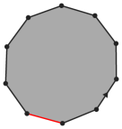
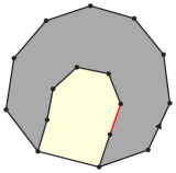
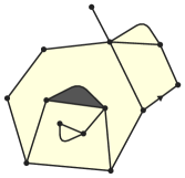
Figure 3: A filled-in exploration of a map with a target face $\mathfrak{m}_{\square}\in\mathcal{M}^{5}_{1}$. The peeled edge is in red, the root face is in white, the target face is in black and the hole containing the target is in grey. At the first step, an event $C_{4}$ happens, then an event $G_{1,*}$ occurs and finally the event $C_{1}^{\mathrm{stop}}$ ends the exploration.

The peeling algorithm $\mathcal{A}$ may be arbitrary, even random, but we require it to be Markovian with respect to the exploration in the sense that, conditionally on the explored region $\overline{\mathfrak{e}}_{n}$, the conditional law of $\mathcal{A}(\overline{\mathfrak{e}}_{n})$ only depends on $\overline{\mathfrak{e}}_{n}$. For instance, the peeled edge may be chosen uniformly at random on the boundary of the hole as in Subsection 3.2 or in such a way that the dual distance from the peeled edge to the root is non-decreasing along the exploration as in Subsection 3.3. During the peeling exploration, one records the evolution of half of the number of edges on the boundary of the hole, which is denoted by $(P_{p}(n))_{n\geq 0}$ if $*\in\{\bullet,\square\}$ and $(P_{\infty}(n))_{n\geq 0}$ if $*=\infty$ and called the perimeter process associated to the exploration. One can express the law of the peeling process (and the law of the perimeter process) under $\mathbb{P}^{(\ell)}_{p}$ or under $\mathbb{P}^{(\ell)}_{\infty}$ using Doob $h$-transforms of the random walk $S=(S_{n})_{n\geq 0}$ of step distribution $\nu$.

Now we recall the law of the filled-in peeling exploration $(\overline{\mathfrak{e}}_{n})_{n\geq 0}$ under $\mathbb{P}^{(\ell)}_{p}$ or under $\mathbb{P}^{(\ell)}_{\infty}$, as described by Proposition 4.7 from [13] in the case $*=\square,\bullet$ and [8] in the case $*=\infty$ (see also Proposition 7.4 in [13]).

Proposition 3.1.

([13],[8]) Let $\ell,p\geq 1$, let $\mathcal{A}$ be a peeling algorithm and $(\overline{\mathfrak{e}}_{n})_{n\geq 0}$ be the peeling process under $\mathbb{P}_{0}^{(\ell)},\mathbb{P}^{(\ell)}_{p}$ or $\mathbb{P}^{(\ell)}_{\infty}$. Then $(\overline{\mathfrak{e}}_{n})_{n\geq 0}$ is a Markov chain with the following transition probabilities: conditionally on $\overline{\mathfrak{e}}_{n}$, and $P(n)=m\geq 1$ (assuming that the exploration has not stopped yet), the events $C_{k},C_{p}^{\mathrm{stop}}$(for $*=\square$)$,G_{k,*}$ and $G_{*,k}$ occur respectively with probabilities

$$\nu(k-1)\frac{h(m+k-1)}{h(m)},\ \nu(-m-p)\frac{h(-p)}{h(m)},\ \frac{1}{2}\nu(-k-1)\frac{h(m-k-1)}{h(m)}\text{ and }\frac{1}{2}\nu(-k-1)\frac{h(m-k-1)}{h(m)},$$

where $h=h^{\downarrow}_{p}$ for $*=\square$, $h=h^{\downarrow}$ for $*=\bullet$ and $h=h^{\uparrow}$ for $*=\infty$. Moreover, conditionally on each event, the holes filled-in during the exploration are independent finite $\bf q$-Boltzmann maps (without target) of corresponding perimeters.

As a consequence, for all $p\geq 0$, the perimeter process under $\mathbb{P}_{p}^{(\ell)}$ (resp. under $\mathbb{P}_{\infty}^{(\ell)}$) indeed corresponds to the Doob $h^{\downarrow}_{p}$-transform killed when it reaches $-p$ (resp. Doob $h^{\uparrow}$-transform) of the walk $S$ started from $\ell$, if we set by convention that the perimeter drops to $-p$ when the exploration stops.

3.2 Uniform peeling and first-passage percolation distance

It is possible to use the peeling process to study the first-passage percolation distance on a map with a target $\mathfrak{m}_{*}$, or an infinite map of the plane. A very convenient algorithm is the uniform peeling algorithm $\mathcal{A}_{\mathrm{uniform}}$ which selects an edge on the boundary of the hole uniformly at random at every step. We refer to [13] 13.1 or [10] 2.4 for details.

This exploration can be related to the fpp distance on $\mathfrak{m}_{*}$ in the following way: for all $t\geq 0$, let $\overline{\mathrm{Ball}}^{\mathrm{fpp}}_{t}(\mathfrak{m}_{*})$ be the sub-map of $\mathfrak{m}_{*}$ obtained by keeping the connected subset of dual edges whose endpoints are at fpp distance at most $t$ from the root face, then by gluing the corresponding faces according to those dual edges and finally by filling in the holes that do not contain the target (the finite holes in the case $*=\infty$). Then the process $(\overline{\mathrm{Ball}}^{\mathrm{fpp}}_{t}(\mathfrak{m}_{*}))_{t\geq 0}$ admits jumps $0=T_{0}<T_{1}<\cdots$. One can check (see Proposition 2.3 in [10]) that for all $n\geq 0$, the sub-map $\overline{\mathrm{Ball}}^{\mathrm{fpp}}_{T_{n+1}}(\mathfrak{m})$ can be obtained from $\overline{\mathrm{Ball}}^{\mathrm{fpp}}_{T_{n}}(\mathfrak{m}_{*})$ by the peeling of a uniform random edge on the boundary of the hole. Furthermore, conditionally on $(\overline{\mathrm{Ball}}^{\mathrm{fpp}}_{T_{n}}(\mathfrak{m}_{*}))_{n\geq 0}$, the random variables $T_{n+1}-T_{n}$ are independent and follow exponential laws of parameter $|\partial\overline{\mathrm{Ball}}^{\mathrm{fpp}}_{T_{n}}(\mathfrak{m}_{*})|$ where $\partial\overline{\mathrm{Ball}}^{\mathrm{fpp}}_{T_{n}}(\mathfrak{m}_{*})$ is the set of edges on the boundary of $\overline{\mathrm{Ball}}^{\mathrm{fpp}}_{T_{n}}(\mathfrak{m}_{*})$.

From the above results, by coupling the uniform exploration with the exponential variables that define the fpp distance, the fpp distance from the root face to the submap $\mathfrak{u}$ filling the hole of boundary $\partial\overline{\mathfrak{e}}_{n}$ can be written as

$$d_{\mathrm{fpp}}^{\dagger}(f_{r},\mathfrak{u})=T_{n+1}=\sum_{i=0}^{n}\frac{\mathcal{E}_{i}}{|\partial\overline{\mathrm{Ball}}^{\mathrm{fpp}}_{T_{i}}(\mathfrak{m}_{*})|}=\sum_{i=0}^{n}\frac{\mathcal{E}_{i}}{2P(i)},$$ (3.2)

where $P(i)=|\partial\overline{\mathrm{Ball}}^{\mathrm{fpp}}_{T_{i}}(\mathfrak{m})|/2$ is the perimeter process associated to the exploration and the $\mathcal{E}_{i}$ for $i\geq 0$ are i.i.d. exponential random variables of parameter $1$ which are independent from the exploration $(\overline{\mathfrak{e}}_{n})_{n\geq 0}$, and a fortiori from $(P(n))_{n\geq 0}$. In particular, if $\mathfrak{m}_{\square}\in\mathcal{M}^{(\ell)}_{p}$ for $\ell,p\geq 1$ and $n$ is the time at which the target face $\square$ is discovered, i.e. the event $C^{\mathrm{target}}_{p}$ happens at time $n$, or equivalently $\overline{\mathfrak{e}}_{n}=\mathfrak{m}_{\square}$, then $d_{\mathrm{fpp}}^{\dagger}(f_{r},\square)=T_{n}$.

3.3 Peeling by layers and dual graph distance

In the same way, a particular peeling algorithm $\mathcal{A}_{\mathrm{layers}}$ called the peeling by layers algorithm is suited to the study of the dual graph distance on a map with a target $\mathfrak{m}_{*}$ (or an infinite map of the plane). Recall that $d^{\dagger}_{\mathrm{gr}}$ denotes the dual graph distance on a map $\mathfrak{m}$. If $f$ is a face of $\mathfrak{m}$ the distance to the root face $d^{\dagger}_{\mathrm{gr}}(f_{r},f)$ is also called the height of $f$. We can also define the height of an edge $e$ as the minimum of the heights of the faces on both sides of $e$.

The peeling algorithm $\mathcal{A}_{\mathrm{layers}}$, described in [10] 2.3, see also [13] p.185, is defined only on (finite) sub-maps $\overline{\mathfrak{e}}$ of $\mathfrak{m}_{*}$ with a hole (containing the target when $*=\square$) which satisfy the following hypothesis:

1. There exists an integer $h\geq 0$ such that all the edges on the boundary of the hole $\partial\overline{\mathfrak{e}}$ are at height $h$ or $h+1$, and such that the set of edges of $\partial\overline{\mathfrak{e}}$ at heigth $h$ forms a (non empty) segment.

If $\overline{\mathfrak{e}}$ satisfies (H), we then set $\mathcal{A}_{\mathrm{layers}}(\overline{\mathfrak{e}})$ to be the unique edge of $\partial\overline{\mathfrak{e}}$ at height $h$ such that the edge immediately on its left is at height $h+1$. If all the edges of $\partial\overline{\mathfrak{e}}$ are at height $h$ the edge $\mathcal{A}_{\mathrm{layers}}(\overline{\mathfrak{e}})$ is then chosen deterministically.

One can check that on the events $C_{k}$, $G_{*,k}$ and $G_{k,*}$ the sub-map obtained after peeling $\mathcal{A}_{\mathrm{layers}}(\overline{\mathfrak{e}})$ satisfies (H) again. Moreover, $\overline{\mathfrak{e}}_{0}$ satisfies (H) as well. Thus the peeling exploration with algorithm $\mathcal{A}_{\mathrm{layers}}$ is well defined.

For every $n\geq 0$, let $H(n)$ be the minimum of the heights of the edges of $\partial\overline{\mathfrak{e}}_{n}$. Then $H(0)=0$ and for all $n\geq 0$, we have $\Delta H(n)\coloneqq H(n+1)-H(n)\in\{0,1\}$. One has $\Delta H(n)=1$ when all the edges of $\partial\overline{\mathfrak{e}}_{n+1}$ are at height $H(n)+1$. The process $H(n)$ is called the height process associated to the peeling by layers exploration. The integer $H(n)+1$ can also be seen as the height of the hole in $\overline{\mathfrak{e}}_{n}$. In particular, if $\mathfrak{m}_{\square}\in\mathcal{M}^{(\ell)}_{p}$ for some $\ell,p\geq 1$ and $n$ is the first time such that $\overline{\mathfrak{e}}_{n}=\mathfrak{m}_{\square}$, then $d_{\mathrm{gr}}^{\dagger}(f_{r},\square)=H(n-1)+1$.

3.4 Exchanging the root and the target

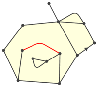
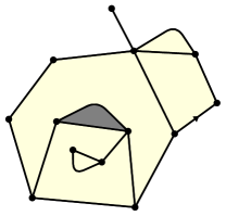
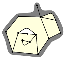
Figure 4: From left to right: a map with a distinguished edge in red, the same map with the edge “unzipped” giving rise to a distinguished $2$-face (in grey) and finally the same map which has been re-rooted.

In order to study the distance from the root face to a uniform random face of $\mathfrak{M}^{(\ell)}$, we will first look at the distance between the root face and a uniform random edge $E$ in $\mathfrak{M}^{(\ell)}$. We will then come back to a uniform random face using a biasing argument in Subsection 4.3. This distance is defined as the minimum of the distances from the root face to a face next to this edge. By unzipping the uniform random edge and thus creating a distinguished face of degree $2$, one can see that the map obtained from $\mathfrak{M}^{(\ell)}$ belongs to $\mathcal{M}_{1}^{(\ell)}$. We denote this map by $\widetilde{\mathfrak{M}}_{1}^{(\ell)}$.

Remark 3.2.

This unzipping operation does not modify the distances so much. More precisely, the graph distance $d^{\dagger}_{\mathrm{gr}}(f_{r},\square)$ in $\widetilde{\mathfrak{M}}_{1}^{(\ell)}$ equals $d^{\dagger}_{\mathrm{gr}}(f_{r},E)+1$ in $\mathfrak{M}^{(\ell)}$ while $d^{\dagger}_{\mathrm{fpp}}(f_{r},\square)$ in $\widetilde{\mathfrak{M}}_{1}^{(\ell)}$ is lower bounded by $d^{\dagger}_{\mathrm{fpp}}(f_{r},E)$ and is upper bounded by $d^{\dagger}_{\mathrm{fpp}}(f_{r},E)+\mathcal{E}$ in $\mathfrak{M}^{(\ell)}$ where $\mathcal{E}$ is an independent exponential variable of parameter $1$.

Besides, one can notice that exchanging the roles of the root face and of the target face by choosing a root edge on the former target face does not modify the distance between the root face and the target face. All the operations we did are illustrated by Figure 4. This swap between the root face and the target face will be useful insofar as in the next subsection we will introduce a coupling of $\mathbb{P}_{\ell}^{(1)}$ with $\mathbb{P}^{(1)}_{\infty}$ that will enable us to use the results of [11]. Let $\widetilde{\mathfrak{M}}_{\ell}^{(1)}$ be the map obtained from $\widetilde{\mathfrak{M}}_{1}^{(\ell)}$ by exchanging the root face and the target face and choosing the root edge uniformly at random around the new root face.

So as to transfer our results under $\mathbb{P}^{(1)}_{\ell}$ to the map $\mathfrak{M}^{(\ell)}$ equipped with a random uniform edge $E$, we state the following lemma.

Lemma 3.3.

If $(\varphi_{\ell})_{\ell\geq 1}$ is a sequence of functions from $\mathcal{M}^{(1)}_{\ell}$ to $\mathbb{R}_{+}$ uniformly bounded by a constant $C>0$ such that

$$\mathbb{E}^{(1)}_{\ell}\varphi_{\ell}(\mathfrak{m}_{\square})\mathop{\longrightarrow}\limits_{\ell\to\infty}0,$$

then

$$\mathbb{E}\varphi_{\ell}\left(\widetilde{\mathfrak{M}}_{\ell}^{(1)}\right)\mathop{\longrightarrow}\limits_{\ell\to\infty}0.$$

In particular, if $(A_{\ell})_{\ell\geq 1}$ is a sequence of subsets of $\mathcal{M}^{(1)}_{\ell}$ such that $\mathbb{P}^{(1)}_{\ell}(A_{\ell})\to 0$ as $\ell\to\infty$, then $\mathbb{P}(\widetilde{\mathfrak{M}}_{\ell}^{(1)}\in A_{\ell})\to 0$.

Proof.

Observe first that the law of $\widetilde{\mathfrak{M}}_{1}^{(\ell)}$ can be characterized using $\mathbb{P}^{(\ell)}_{1}$. Indeed, if $\mathfrak{m}_{\square}\in\mathcal{M}_{1}^{(\ell)}$ is obtained by unzipping an edge of a map $\mathfrak{m}^{\prime}\in\mathcal{M}^{(\ell)}$, then

$$\mathbb{P}(\widetilde{\mathfrak{M}}_{1}^{(\ell)}=\mathfrak{m}_{\square}) =\frac{1}{\#\mathrm{Edges}(\mathfrak{m}^{\prime})}\mathbb{P}(\mathfrak{M}^{(\ell)}=\mathfrak{m}^{\prime})=\frac{1}{\#\mathrm{Edges}(\mathfrak{m}^{\prime})}\frac{w_{\bf q}(\mathfrak{m}^{\prime})}{W^{(\ell)}}$$

$$=\frac{1}{\#\mathrm{Edges}(\mathfrak{m}_{\square})-1}\frac{W^{(\ell)}_{1}}{W^{(\ell)}}\frac{w_{\bf q}(\mathfrak{m}_{\square})}{W^{(\ell)}_{1}}=\frac{W^{(\ell)}_{1}}{W^{(\ell)}}\frac{1}{\#\mathrm{Edges}(\mathfrak{m}_{\square})-1}\mathbb{P}^{(\ell)}_{1}(\mathfrak{m}_{\square}).$$

Another well known and useful consequence of this unzipping operation is that

$$\mathbb{E}\,\#\mathrm{Edges}(\mathfrak{M}^{(\ell)})=\frac{W_{1}^{(\ell)}}{W^{(\ell)}}\mathop{\sim}\limits_{\ell\to\infty}\frac{\frac{1}{2}h^{\downarrow}_{1}(\ell)c_{\bf q}^{\ell+1}}{\frac{p_{\bf q}}{2}c_{\bf q}^{\ell+1}\ell^{-2}}\mathop{\sim}\limits_{\ell\to\infty}b_{\bf q}\ell^{3/2}\text{ where }b_{\bf q}=\frac{1}{2p_{\bf q}\sqrt{\pi}},$$ (3.3)

applying successively (1.1), (3.1), (2.1) and the fact that $h^{\downarrow}(\ell)\sim 1/\sqrt{\pi\ell}$.

Next, the law of $\widetilde{\mathfrak{M}}_{\ell}^{(1)}$ can be expressed as follows. Let $\mathfrak{m}_{\square}\in\mathcal{M}^{(1)}_{\ell}$ which is obtained by re-rooting a map $\mathfrak{m}^{\prime}_{\square}\in\mathcal{M}^{(\ell)}_{1}$. Then one can check that

$$\mathbb{P}\left(\widetilde{\mathfrak{M}}_{\ell}^{(1)}=\mathfrak{m}_{\square}\right)=\frac{2\ell}{2}\mathbb{P}\left(\widetilde{\mathfrak{M}}_{1}^{(\ell)}=\mathfrak{m}^{\prime}_{\square}\right)=\frac{2\ell}{2}\frac{W^{(\ell)}_{1}}{W^{(\ell)}}\frac{\mathbb{P}^{(\ell)}_{1}(\mathfrak{m}^{\prime}_{\square})}{\#\mathrm{Edges}(\mathfrak{m}^{\prime}_{\square})-1}=\frac{W^{(\ell)}_{1}}{W^{(\ell)}}\frac{\mathbb{P}^{(1)}_{\ell}(\mathfrak{m}_{\square})}{\#\mathrm{Edges}(\mathfrak{m}_{\square})-1}.$$ (3.4)

We deduce that

$$\mathbb{E}\varphi_{\ell}\left(\widetilde{\mathfrak{M}}_{\ell}^{(1)}\right)=\sum_{\mathfrak{m}_{\square}\in\mathcal{M}^{(1)}_{\ell}}\frac{W^{(\ell)}_{1}}{W^{(\ell)}}\frac{\mathbb{P}^{(1)}_{\ell}(\mathfrak{m}_{\square})}{\#\mathrm{Edges}(\mathfrak{m}_{\square})-1}\varphi_{\ell}(\mathfrak{m}_{\square})=\frac{W^{(\ell)}_{1}}{W^{(\ell)}}\mathbb{E}^{(1)}_{\ell}\left(\frac{\varphi_{\ell}(\mathfrak{m}_{\square})}{\#\mathrm{Edges}(\mathfrak{m}_{\square})-1}\right).$$ (3.5)

Let $\varepsilon>0$. We next distinguish whether the number of edges is larger than $\varepsilon\ell^{3/2}+1$ or not. On the one hand, using (3.3), one can see that

$$\frac{W^{(\ell)}_{1}}{W^{(\ell)}}\mathbb{E}^{(1)}_{\ell}\left(\frac{\varphi_{\ell}(\mathfrak{m}_{\square})}{\#\mathrm{Edges}(\mathfrak{m}_{\square})-1}{\bf 1}_{\#\mathrm{Edges}(\mathfrak{m}_{\square})\geq\varepsilon\ell^{3/2}+1}\right)\leq\frac{W^{(\ell)}_{1}}{\varepsilon\ell^{3/2}W^{(\ell)}}\mathbb{E}^{(1)}_{\ell}f(\mathfrak{m}_{\square})\mathop{\longrightarrow}\limits_{\ell\to\infty}0.$$

On the other hand,

$$\frac{W^{(\ell)}_{1}}{W^{(\ell)}}\mathbb{E}^{(1)}_{\ell}\left(\frac{\varphi_{\ell}(\mathfrak{m}_{\square}){\bf 1}_{\#\mathrm{Edges}(\mathfrak{m}_{\square})\leq\varepsilon\ell^{3/2}}}{\#\mathrm{Edges}(\mathfrak{m}_{\square})-1}\right) \leq\frac{W^{(\ell)}_{1}}{W^{(\ell)}}\mathbb{E}^{(1)}_{\ell}\left(C\frac{{\bf 1}_{\#\mathrm{Edges}(\mathfrak{m}_{\square})\leq\varepsilon\ell^{3/2}}}{\#\mathrm{Edges}(\mathfrak{m}_{\square})-1}\right)$$

$$=C\mathbb{P}\left(\#\mathrm{Edges}\left(\widetilde{\mathfrak{M}}_{\ell}^{(1)}\right)\leq\varepsilon\ell^{3/2}\right)\text{\enskip by (\ref{eq preuve lemme racine}) }$$

$$=C\mathbb{P}(\#\mathrm{Edges}(\mathfrak{M}^{(\ell)})\leq\varepsilon\ell^{3/2}-1).$$

Furthermore,

$$\lim_{\varepsilon\to 0}\limsup_{\ell\to\infty}\mathbb{P}^{(\ell)}(\#\mathrm{Edges}(\mathfrak{m})\leq\varepsilon\ell^{3/2}-1)=0,$$

since $\#\mathrm{Edges}(\mathfrak{M}^{(\ell)})\ell^{-3/2}$ converges in distribution towards a positive random variable as $\ell\to\infty$, see e.g. Proposition 10.4 in [13]. ∎

4 Scaling limit of the distance to a target

This section and the rest of this paper are devoted to the study of the dual distances on the $3/2$-stable map $\mathfrak{M}^{(\ell)}$ of perimeter $2\ell$. We thus henceforth assume that $\bf q$ is non-generic critical of type $a=2$. We will drop the subscript $2$ in $\Upsilon_{2}$, $\Upsilon^{\uparrow}_{2}$, $\Upsilon^{\downarrow}_{2}$ and $\Upsilon^{\downarrow}_{-1,2}$.

As announced before, we first study the distance from the root face to a uniform random edge of $\mathfrak{M}^{(\ell)}$ and then transpose the result to the distance to a uniform random face and to a uniform random vertex. From Subsection 3.4, it suffices to study the distance from the root face $f_{r}$ to the target face $\square$ under $\mathbb{P}^{(1)}_{\ell}$. Thus, we may use the filled-in exploration of $\mathbb{P}^{(1)}_{\ell}$ presented in Section 3 with in particular the peeling algorithms $\mathcal{A}_{\mathrm{uniform}}$ and $\mathcal{A}_{\mathrm{layers}}$.

4.1 The first-passage percolation distance to a uniform random edge in $\mathfrak{M}^{(\ell)}$

From Subsection 3.2, in particular (3.2), we know that the fpp distance from the root face $f_{r}$ to the target face $\square$ under $\mathbb{P}_{\ell}^{(1)}$ is

$$d_{\text{fpp}}^{\dagger}(f_{r},\square)=\sum_{k=0}^{\tau_{-\ell}-1}{\mathcal{E}_{k}\over 2P_{\ell}(k)},$$ (4.1)

where the $\mathcal{E}_{k}$’s are i.i.d. exponential random variables of parameter one independent of the perimeter process. The properties of the perimeter process proved in Section 2 enable us to state the following proposition, taking us closer to the first convergence of Theorem 1.1.

Proposition 4.1.

Under $\mathbb{P}_{\ell}^{(1)}$,

$${d_{\mathrm{fpp}}^{\dagger}(f_{r},\square)\over\log\ell}\mathop{\longrightarrow}\limits_{\ell\to\infty}^{(\mathbb{P})}{1\over\pi^{2}p_{\bf q}}.$$

As a consequence, if $E^{(\ell)}$ is a uniform edge in $\mathfrak{M}^{(\ell)}$, then

$${d_{\mathrm{fpp}}^{\dagger}(f_{r},E^{(\ell)})\over\log\ell}\mathop{\longrightarrow}\limits_{\ell\to\infty}^{(\mathbb{P})}{1\over\pi^{2}p_{\bf q}}.$$

Proof.

For the first convergence, it suffices to prove that

$${1\over\log\ell}\sum_{k=0}^{\tau_{-\ell}-1}{1\over 2P_{\ell}(k)}\mathop{\longrightarrow}\limits_{\ell\to\infty}^{(\mathbb{P})}{1\over\pi^{2}p_{\bf q}}.$$ (4.2)

Indeed, assuming (4.2), like in the beginning of the proof of Proposition 3 of [11], we can reason conditionally on $P_{\ell}$:

$$\mathbb{E}\left(\left.\left({1\over\log\ell}\sum_{k=0}^{\tau_{-\ell}-1}{\mathcal{E}_{k}-1\over 2P_{\ell}(k)}\right)^{2}\right|P_{\ell}\right)={1\over(\log\ell)^{2}}\sum_{k=0}^{\tau_{-\ell}-1}{1\over 4P_{\ell}(k)^{2}}\leq{1\over(\log\ell)^{2}}\sum_{k=0}^{\tau_{-\ell}-1}{1\over 4P_{\ell}(k)}\mathop{\longrightarrow}\limits_{\ell\to\infty}^{(\mathbb{P})}0,$$

where the convergence comes from (4.2). In order to prove (4.2), one can first see that by Theorem 2.8, for all $\varepsilon>0$,

$$\sum_{k=\lfloor\varepsilon\ell\rfloor}^{\tau_{-\ell}-1}{1\over 2P_{\ell}(k)}\mathop{\longrightarrow}\limits_{\ell\to\infty}^{(\mathrm{d})}\int_{\varepsilon}^{\tilde{\tau}}\frac{1}{2\Upsilon^{\downarrow}_{-1}(p_{\bf q}t)}dt.$$ (4.3)

Besides, under the coupling $\mathbb{P}^{(1),\lfloor\varepsilon\ell\rfloor}_{\ell,\infty}$ of Lemma 2.5, on the event $\tau_{-\ell}>\lfloor\varepsilon\ell\rfloor$ (which holds with probability greater than $1-o(1)$ uniformly in $\ell$ as $\varepsilon\to 0$), for all $k\leq\lfloor\varepsilon\ell\rfloor$ we have $P_{\ell}(k)=P_{\infty}(k)$. Thus, on the event $\tau_{-\ell}>\lfloor\varepsilon\ell\rfloor$, we have

$${1\over\log\ell}\sum_{k=0}^{\lfloor\varepsilon\ell\rfloor}{1\over 2P_{\ell}(k)}={1\over\log\ell}\sum_{k=0}^{\lfloor\varepsilon\ell\rfloor}{1\over 2P_{\infty}(k)}\mathop{\longrightarrow}\limits_{\ell\to\infty}^{(\mathbb{P})}{1\over\pi^{2}p_{\bf q}},$$

by Equation (15) of [11]. Consequently, combining this convergence with (4.3), we can conclude that (4.2) holds, which ends the proof of the first convergence.

The first convergence of the statement is immediately transferred to the map $\mathfrak{M}^{(\ell)}$ equipped with a uniform edge by Remark 3.2 and by Lemma 3.3, using the function $\varphi_{\ell}$ defined by

$$\forall\mathfrak{m}_{\square}\in\mathcal{M}^{(1)}_{\ell},\qquad\varphi_{\ell}(\mathfrak{m}_{\square})=\mathbb{E}\left(\left|\frac{d_{\mathrm{fpp}}^{\dagger}(f_{r},\square)}{\log\ell}-\frac{1}{\pi^{2}p_{\bf q}}\right|\wedge 1\right),$$

where the expectation applies to the exponential weights defining the fpp distance. ∎

4.2 The dual graph distance to a uniform random edge in $\mathfrak{M}^{(\ell)}$

The height process along the filled-in exploration using the peeling by layers algorithm of a map under $\mathbb{P}_{\ell}^{(1)}$ is denoted by $H_{\ell}$. We recall that $H_{\ell}(n)$ is the smallest height of an edge in $\partial\overline{\mathfrak{e}}_{n}$. From Subsection 3.3, we know that the dual graph distance from the root face $f_{r}$ to the target face $\square$ under $\mathbb{P}_{\ell}^{(1)}$ is $d_{\mathrm{gr}}^{\dagger}(f_{r},\square)=H_{\ell}(\tau_{-\ell}-1)+1$.

Now we can state and prove the main result of this section, which gives the asymptotic behavior of the dual graph distance from the root face to the target face under $\mathbb{P}^{(1)}_{\ell}$, and brings us closer to the second convergence of Theorem 1.1 by the arguments of Subsection 3.4.

Proposition 4.2.

Under $\mathbb{P}^{(1)}_{\ell}$,

$${d_{\mathrm{gr}}^{\dagger}(f_{r},\square)\over(\log\ell)^{2}}\mathop{\longrightarrow}\limits_{\ell\to\infty}^{(\mathbb{P})}{1\over 2\pi^{2}}.$$

As a consequence, if $E^{(\ell)}$ is a uniform random edge of $\mathfrak{M}^{(\ell)}$, then, in $\mathfrak{M}^{(\ell)}$,

$${d_{\mathrm{gr}}^{\dagger}(f_{r},E^{(\ell)})\over(\log\ell)^{2}}\mathop{\longrightarrow}\limits_{\ell\to\infty}^{(\mathbb{P})}{1\over 2\pi^{2}}.$$

Proof.

First of all, from Proposition 3.1, it is easy to see that for all $n\geq 1$, for any increasing sequence of maps with holes $\mathfrak{u}_{0}\subset\mathfrak{u}_{1}\subset\cdots\subset\mathfrak{u}_{n-1}$,

$$\mathbb{P}_{\ell}^{(1)} (\mathfrak{e}_{0}=\mathfrak{u}_{0},\ldots,\mathfrak{e}_{n-1}=\mathfrak{u}_{n-1}|\tau_{-\ell}=n\text{ and }P_{\ell}({n-1})=|\partial\mathfrak{u}_{n-1}|/2)$$

$$=\mathbb{P}_{\infty}^{(1)}(\mathfrak{e}_{0}=\mathfrak{u}_{0},\ldots,\mathfrak{e}_{n-1}=\mathfrak{u}_{n-1}|P_{\infty}(n-1)=|\partial\mathfrak{u}_{n-1}|/2).$$

As a result, if $F:\mathbb{R}\to\mathbb{R}$ is a continuous bounded function,

$$\mathbb{E}^{(1)}_{\ell}F\left(\frac{H_{\ell}(\tau_{-\ell}-1)}{(\log\ell)^{2}}\right) =\sum_{n,k\geq 1}\mathbb{E}_{\infty}^{(1)}\left(\left.F\left(\frac{H_{\infty}(\tau_{-\ell}-1)}{(\log\ell)^{2}}\right)\right|P_{\infty}(n-1)=k\right)\mathbb{P}_{\ell}^{(1)}\left(\tau_{-\ell}=n,P_{\ell}(n-1)=k\right)$$

We take $F:x\mapsto|x-1/(2\pi^{2})|\wedge 1$. Let $\varepsilon>0$. Let $\delta>0$ be small enough so that for all $\ell\geq 1$, under $\mathbb{P}^{(1)}_{\ell}$, we have $\tau_{-\ell}/\ell\in[\delta,1/\delta]$ and $P_{\ell}(\tau_{-\ell}-1)/\ell\in[\delta,1/\delta]$ with probability at least $1-\varepsilon$. Such a $\delta$ exists thanks to Proposition 2.7. Then, by Proposition 2.7 and Lemma 2.3, uniformly on $s,u\in[\delta,1/\delta]$ as $\ell\to\infty$,

$$\frac{\mathbb{P}^{(1)}_{\ell}(\tau_{-\ell}=\lfloor\ell s\rfloor\text{ and }P_{\ell}(\lfloor\ell s\rfloor-1)=\lfloor\ell u\rfloor)}{\mathbb{P}_{\infty}^{(1)}(P_{\infty}(\lfloor\ell s\rfloor-1)=\lfloor\ell u\rfloor)} =\frac{\mathbb{P}^{(1)}_{\ell}(\tau_{-\ell}=\lfloor\ell s\rfloor\text{ and }P_{\ell}(\lfloor\ell s\rfloor-1)=\lfloor\ell u\rfloor)}{(h^{\uparrow}(\lfloor\ell u\rfloor)/h^{\uparrow}(1))\mathbb{P}_{1}(S_{1},\ldots,S_{\lfloor\ell s\rfloor-1}\geq 1\text{ and }S_{\lfloor\ell s\rfloor-1}=\lfloor\ell u\rfloor)}$$

$$\sim\frac{\pi p_{\bf q}}{\ell\sqrt{u}(1+u)^{2}},$$

where we used that $h^{\uparrow}(\ell)\sim 2\sqrt{\ell/\pi}$. In particular, the above ratio is uniformly bounded in $\ell\geq 1$ and $u,s\in[\delta,1/\delta]$ by a constant $C(\delta)$ times $1/\ell$. Thus

$$\mathbb{E}^{(1)}_{\ell}F\left(\frac{H_{\ell}(\tau_{-\ell}-1)}{(\log\ell)^{2}}\right) \leq\varepsilon+C(\delta)\ell^{-1}\int_{\delta}^{1/\delta}ds\int_{\delta}^{1/\delta}du\ell^{2}\mathbb{E}^{(1)}_{\infty}\left(F\left(\frac{H_{\infty}(\lfloor\ell s\rfloor-1)}{(\log\ell)^{2}}\right){\bf 1}_{P_{\infty}(\lfloor\ell s\rfloor-1)=\lfloor\ell u\rfloor}\right)$$

$$\leq\varepsilon+C(\delta)\int_{\delta}^{1/\delta}ds\mathbb{E}^{(1)}_{\infty}\left(F\left(\frac{H_{\infty}(\lfloor\ell s\rfloor-1)}{(\log\ell)^{2}}\right)\right).$$

The last integral tends to $0$ as $\ell\to+\infty$ because of Proposition 4 from [11], stating that under $\mathbb{P}_{\infty}^{(1)}$,

$${H_{\infty}(\ell)\over(\log\ell)^{2}}\mathop{\longrightarrow}\limits_{\ell\to\infty}^{(\mathbb{P})}{1\over 2\pi^{2}}.$$

This entails the first convergence.

The second convergence is a straightforward consequence of the first one due to Remark 3.2 and to Lemma 3.3, using the function $\varphi_{\ell}$ defined by

$$\forall\mathfrak{m}_{\square}\in\mathcal{M}^{(1)}_{\ell},\qquad\varphi_{\ell}(\mathfrak{m}_{\square})=\left|\frac{d_{\mathrm{gr}}^{\dagger}(f_{r},\square)}{(\log\ell)^{2}}-\frac{1}{2\pi^{2}}\right|\wedge 1.$$

This concludes the proof. ∎

4.3 Replacing the uniform random edge by a vertex or a face

Let us explain how the results of the preceding subsections also give us the distance from the root face to a uniform random vertex or to a uniform random face, hence proving Theorem 1.1 at the end of this subsection. This subsection relies on classical arguments involving the peeling exploration and bijections with trees which may be skipped by the reader.

We first focus on the case of a uniform random vertex. Notice that $|\mathrm{Vertices}(\mathfrak{M}^{(\ell)})|=\sum_{\vec{e}}{1\over\deg v(\vec{e})}$, where the sum is over all the oriented edges $\vec{e}$ of $\mathfrak{M}^{(\ell)}$. To get a uniform random vertex on $\mathfrak{M}^{(\ell)}$, conditionally on $\mathfrak{M}^{(\ell)}$, we pick a random oriented edge $\vec{E}$ of $\mathfrak{M}^{(\ell)}$ of law

$$\forall\vec{e}\in\mathrm{Edges}(\mathfrak{M}^{(\ell)}),\ \ \mathbb{P}\left(\left.\vec{E}=\vec{e}\ \right|\mathfrak{M}^{(\ell)}\right)\coloneqq{1\over\deg v(\vec{e})}{1\over|\mathrm{Vertices}(\mathfrak{M}^{(\ell)})|},$$ (4.4)

where $v(\vec{e})$ is the vertex from which starts $\vec{e}$. Then for all vertex $v$ of $\mathfrak{M}^{(\ell)}$

$$\mathbb{P}\left(\left.v(\vec{E})=v\right|\mathfrak{M}^{(\ell)}\right)={1\over|\mathrm{Vertices}(\mathfrak{M}^{(\ell)})|},$$ (4.5)

i.e. $V\coloneqq v(\vec{E})$ is a random vertex taken uniformly on $\mathfrak{M}^{(\ell)}$.

Let us control the degree of the root vertex $v_{r}$ (from which starts the root edge) under $\mathbb{P}^{(1)}_{\ell}$. The lemma below is an extension of Lemma 15.6 from [13].

Lemma 4.3.

There exists $c\in(0,1)$ such that for all $\ell,j\geq 1$,

$$\mathbb{P}^{(1)}_{\ell}(\deg v_{r}\geq j)\leq c^{j-2}.$$

Proof.

As in [13] we use the peeling exploration “peeling around the root vertex”, defined as follows: as long as the root vertex belongs to the boundary of the hole $\partial\overline{\mathfrak{e}}_{n}$, we peel the edge on $\partial\overline{\mathfrak{e}}_{n}$ adjacent on the left of $v_{r}$ until it becomes an interior vertex. More precisely, after an event of type $G$, we fill-in the hole which does not have $v_{r}$ on its boundary and we continue the exploration. Thus, the hole may not contain the target after some time. We write $G_{k_{1},k_{2}}$ the event of an identification of two edges on the boundary of a hole of perimeter $2p=2k_{1}+2k_{2}+2$ which does not contain the target, giving rise to a hole of perimeter $2k_{1}$ on the left of the peeled edge (which will be filled-in) and a hole of perimeter $2k_{2}$ on the right. This event has the transition probability $W^{(k_{1})}W^{(k_{2})}/W^{(p)}$. The exploration ends when $v_{r}$ becomes an inner vertex, i.e. after an event of type $G_{*,0}$ or after an event of type $G_{k,0}$ for some $k\geq 0$.

At one step of this peeling exploration, let $2p$ be the perimeter of the hole whose boundary contains $v_{r}$. We distinguish the two possible cases:

• Either $v_{r}$ is in the boundary of the hole containing the target face. In that case, the exploration stops if and only if the event $G_{*,0}$ occurs. And this happens with probability $\frac{1}{2}\nu(-1)\frac{h^{\downarrow}_{\ell}(p-1)}{h^{\downarrow}_{\ell}(p)}$ by Proposition 3.1 (and necessarily $p\geq 2$ so that the hole which contains the target has positive boundary length).

• Either $v_{r}$ is in the boundary of a hole which does not contain the target face. In this case, the exploration stops when the event $G_{p-1,0}$ occurs. This event happens with probability $W^{(p-1)}W^{(0)}/W^{(p)}$.

But one can see by (1.1), (2.1) and since $h^{\downarrow}(\ell)\sim 1/\sqrt{\pi\ell}$ when $\ell\to\infty$ that

$$\frac{W^{(0)}W^{(0)}}{W^{(1)}}\wedge\inf_{\begin{subarray}{c}p\geq 2\\ \ell\geq 1\end{subarray}}\left(\frac{1}{2}\nu(-1)\frac{h^{\downarrow}_{\ell}(p-1)}{h^{\downarrow}_{\ell}(p)}\wedge\frac{W^{(p-1)}W^{(0)}}{W^{(p)}}\right)>0.$$

Besides, in the first case, when $p=1$ we automatically have $p\geq 1$ at the next step by an event of type $C_{k}$, and with positive probability we will have $p\geq 2$ at the next step. Moreover, at each step of the exploration, $\deg(v_{r})$ only increases by zero or one, hence the statement of the lemma. ∎

We now recall a lemma which gathers some well known consequences of the Bouttier-Di Francesco-Guitter bijection (from [6]) and Janson & Stefánsson’s trick (from [19] Section 3), together with the Łukasiewicz path.

Lemma 4.4.

([6],[19]) The measure $\mu$ on $\mathbb{Z}_{\geq-1}$ defined by

$$\mu(-1)=\frac{4}{c_{\bf q}}\qquad\text{and}\qquad\mu(k)=q_{k+1}\binom{2k+1}{k+1}(c_{\bf q}/4)^{k}\text{ for all }k\geq 0.$$

is a probability measure. Moreover, to a map $\mathfrak{m}_{\bullet}$ under $\mathbb{P}^{(\ell)}_{0}$ we can associate a random walk $(Y_{n})_{n\geq 0}$ of step distribution $\mu$ starting at zero and stopped when it attains $-\ell$ such that if we denote by $\tau_{-\ell}(Y)$ the time at which $Y$ reaches $-\ell$, then

$$\left\{\begin{array}[]{l}\#\left\{n\in[\![0,\tau_{-\ell}(Y)-1]\!];\ Y_{n+1}-Y_{n}=-1\right\}+1=\#\mathrm{Vertices}(\mathfrak{m}_{\bullet})\\ \#\left\{n\in[\![0,\tau_{-\ell}(Y)-1]\!];\ Y_{n+1}-Y_{n}\neq-1\right\}+1=\#\mathrm{Faces}(\mathfrak{m}_{\bullet}).\end{array}\right.$$

As a consequence $\tau_{-\ell}(Y)=\#\mathrm{Edges}(\mathfrak{m}_{\bullet})$.

Using the previous lemmas, we are able to control the degree of a random uniform vertex in the map $\mathfrak{M}^{(\ell)}$. The degree of a uniform random vertex of the map $\mathfrak{M}^{(\ell)}$ is stochastically dominated by a random variable whose law does not depend on $\ell$:

Lemma 4.5.

There exists $C>0$ and $c\in(0,1)$ such that for all $k,\ell\geq 1$, if $V$ is a uniform random vertex of $\mathfrak{M}^{(\ell)}$, then

$$\mathbb{P}(\deg(V)=k)\leq Cc^{k}.$$

Proof.

Let $\ell\geq 1$ and $\varepsilon>0$. Let $K>0$ whose value will be chosen later. For $k\geq 1$,

$$\mathbb{P}(\deg(V)=k)= \mathbb{P}(\deg(V)=k\text{ and }K|\mathrm{Vertices}(\mathfrak{M}^{(\ell)})|\geq|\mathrm{Edges}(\mathfrak{M}^{(\ell)})|)$$ (4.6)

$$+\mathbb{P}(\deg(V)=k\text{ and }K|\mathrm{Vertices}(\mathfrak{M}^{(\ell)})|<|\mathrm{Edges}(\mathfrak{M}^{(\ell)})|)$$ (4.7)

For the first term (4.6), if we denote by $\vec{E}^{\prime}$ a uniform oriented edge of $\mathfrak{M}^{(\ell)}$, one can see that for all $k\geq 1$,

$$\mathbb{P} \left(\deg(V)=k\text{ and }K|\mathrm{Vertices}(\mathfrak{M}^{(\ell)})|\geq|\mathrm{Edges}(\mathfrak{M}^{(\ell)})|\right)$$

$$=\mathbb{E}\left({\bf 1}_{K|\mathrm{Vertices}(\mathfrak{M}^{(\ell)})|\geq|\mathrm{Edges}(\mathfrak{M}^{(\ell)})|}\sum_{\vec{e}}{1\over\deg v(\vec{e})}{1\over|\mathrm{Vertices}(\mathfrak{M}^{(\ell)})|}{\bf 1}_{\deg(v(\vec{e}))=k}\right)\text{ by (\ref{eq sommet uniforme})}$$

$$=\mathbb{E}^{(\ell)}\left({\bf 1}_{K|\mathrm{Vertices}(\mathfrak{m})|\geq|\mathrm{Edges}(\mathfrak{m})|}{1\over k|\mathrm{Vertices}(\mathfrak{m})|}\#\{\vec{e};\ \deg v(\vec{e})=k\}\right)$$

$$\leq\mathbb{E}^{(\ell)}\left({\bf 1}_{K|\mathrm{Vertices}(\mathfrak{m})|\geq|\mathrm{Edges}(\mathfrak{m})|}{2|\mathrm{Edges}(\mathfrak{m})|\over k|\mathrm{Vertices}(\mathfrak{m})|}\mathbb{P}(\deg(v(\vec{E}^{\prime}))=k|\mathfrak{M}^{(\ell)}=\mathfrak{m})\right)$$

$$\leq\mathbb{E}^{(\ell)}\left(2K\mathbb{P}(\deg(v(\vec{E}^{\prime}))=k|\mathfrak{M}^{(\ell)}=\mathfrak{m})\right)$$

$$=2K\mathbb{P}_{\ell}^{(1)}(\deg(v_{r})=k)$$

$$\leq 2Kc^{k-2}\text{ by Lemma \ref{degré arête},}$$

with $C>0$ and $c\in(0,1)$ independent of $\ell$. We now focus on the second term (4.7).

$$\mathbb{P} \left(\deg(V)=k\text{ and }K|\mathrm{Vertices}(\mathfrak{M}^{(\ell)})|<|\mathrm{Edges}(\mathfrak{M}^{(\ell)})|\right)$$

$$\leq\mathbb{P}\left(|\mathrm{Edges}(\mathfrak{M}^{(\ell)})|\geq k\text{ and }K|\mathrm{Vertices}(\mathfrak{M}^{(\ell)})|<|\mathrm{Edges}(\mathfrak{M}^{(\ell)})|\right).$$

Let $Y$ be the $\mu$-random walk stopped when it attains $-\ell$ associated to $\mathfrak{m}_{\bullet}$ under $\mathbb{P}_{0}^{(\ell)}$ by Lemma 4.4. We also know that $\tau_{-\ell}(Y)=|\mathrm{Edges}(\mathfrak{m})|$ and $D\coloneqq\#\{i\in[\![0,\tau_{-\ell}(Y)-1]\!];\ Y_{i+1}-Y_{i}=-1\}+1=|\mathrm{Vertices}(\mathfrak{m})|$. Thus, by biasing by the number of vertices, we obtain that

$$\mathbb{P} \left(|\mathrm{Edges}(\mathfrak{M}^{(\ell)})|\geq k\text{ and }K|\mathrm{Vertices}(\mathfrak{M}^{(\ell)})|<|\mathrm{Edges}(\mathfrak{M}^{(\ell)})|\right)$$

$$=\frac{1}{W^{(\ell)}}\sum_{\mathfrak{m}\in\mathcal{M}^{(\ell)}}w_{\bf q}(\mathfrak{m}){\bf 1}_{|\mathrm{Edges}(\mathfrak{m})|\geq k\text{ and }K|\mathrm{Vertices}(\mathfrak{m})|<|\mathrm{Edges}(\mathfrak{m})|}$$

$$=\frac{W^{(\ell)}_{0}}{W^{(\ell)}}\mathbb{E}^{(\ell)}_{0}\left(\frac{1}{|\mathrm{Vertices}(\mathfrak{m_{\bullet}})|}{\bf 1}_{|\mathrm{Edges}(\mathfrak{m}_{\bullet})|\geq k\text{ and }K|\mathrm{Vertices}(\mathfrak{m}_{\bullet})|<|\mathrm{Edges}(\mathfrak{m}_{\bullet})|}\right)$$

$$=\frac{W^{(\ell)}_{0}}{W^{(\ell)}}\mathbb{E}\left(\frac{1}{D}{\bf 1}_{KD\leq\tau_{-\ell}(Y)\text{ and }\tau_{-\ell}(Y)\geq k}\right)$$

$$=\frac{W^{(\ell)}_{0}}{W^{(\ell)}}\mathbb{E}\left(\frac{1}{D}\mathbb{P}\left(\left.KD\leq\tau_{-\ell}(Y)\text{ and }\tau_{-\ell}(Y)\geq k\right|D\right)\right).$$

Let us upper bound the conditional probability inside the expectation. One can note that the random walk $Y$ can be built by first sampling the non-zero steps and then inserting between these steps a geometric number (starting at zero, of parameter $1-\mu(0)$) of zero steps (when $\mu(0)=0$, we do not insert any such zero step). Moreover the number of positive steps before $\tau_{-\ell}(Y)$ is smaller than $D$. Thus one can write

$$\tau_{-\ell}(Y)\leq 2D+\sum_{i=1}^{2D}\mathcal{G}_{i},$$

where the $\mathcal{G}_{i}$ are geometric i.i.d. random variables of parameter $1-\mu(0)$, where by convention $\mathcal{G}_{i}=0$ when $\mu(0)=0$. Let $\beta=(1-\mu(0))/(2(3-\mu(0)))$ so that $1-2\beta=4\beta/(1-\mu(0))$. We will distinguish whether $D\geq\beta k$ or not. On the one hand, if $D\leq\beta$, then

$$\mathbb{P}\left(\left.KD\leq\tau_{-\ell}(Y)\text{ and }\tau_{-\ell}(Y)\geq k\right|D\right){\bf 1}_{D\leq\beta k} \leq\mathbb{P}\left(\left.\tau_{-\ell}(Y)\geq k\right|D\right){\bf 1}_{D\leq\beta k}$$

$$\leq\mathbb{P}\left(\left.2D+\sum_{i=1}^{2D}\mathcal{G}_{i}\geq k\right|D\right){\bf 1}_{D\leq\beta k}$$

$$\leq\mathbb{P}\left(\sum_{i=1}^{2\beta k}\mathcal{G}_{i}\geq(1-2\beta)k\right)$$

$$\leq C^{\prime}(c^{\prime})^{k},$$

for $C^{\prime}>0$, $c^{\prime}\in(0,1)$ which do not depend on $\ell$, where the last inequality comes from the large deviations for sums of i.i.d. geometric variables. On the other hand, when $D\geq\beta k$, by choosing $K\geq 2+4/(1-\mu(0))$,

$$\mathbb{P}\left(\left.KD\leq\tau_{-\ell}(Y)\text{ and }\tau_{-\ell}(Y)\geq k\right|D\right){\bf 1}_{D\geq\beta k} =\mathbb{P}\left(\left.KD\leq\tau_{-\ell}(Y)\right|D\right){\bf 1}_{D\geq\beta k}$$

$$\leq\mathbb{P}\left(\left.(K-2)D\leq\sum_{i=1}^{2D}\mathcal{G}_{i}\right|D\right){\bf 1}_{D\geq\beta k}$$

$$\leq C^{\prime}(c^{\prime})^{D}{\bf 1}_{D\geq\beta k}\leq C^{\prime}(c^{\prime})^{\beta k},$$

by the same large deviations. This ends the proof since $\mathbb{E}({1}/{D})=\mathbb{E}^{(\ell)}_{0}({1}/{|\mathrm{Vertices}(\mathfrak{m})|})={W^{(\ell)}}/{W^{(\ell)}_{0}}$ and thus

$$\frac{W^{(\ell)}_{0}}{W^{(\ell)}}\mathbb{E}\left(\frac{1}{D}\mathbb{P}\left(\left.KD\leq\tau_{-\ell}(Y)\text{ and }\tau_{-\ell}(Y)\geq k\right|D\right)\right)\leq C^{\prime}(c^{\prime})^{\beta k},$$

hence the upper bound of the statement. ∎

If $v$ is a vertex of $\mathfrak{m}$, and if $d^{\dagger}$ is a distance on $\mathfrak{m}^{\dagger}$, we define $d^{\dagger}(f_{r},v)$ as the smallest distance from $f_{r}$ to a face $f$ next to $v$.

Proposition 4.6.

If for all $\ell\geq 1$, $V^{(\ell)}$ is a random uniform vertex of $\mathfrak{M}^{(\ell)}$, then

$$\frac{d_{\mathrm{gr}}^{\dagger}(f_{r},V^{(\ell)})}{(\log\ell)^{2}}\mathop{\longrightarrow}\limits_{\ell\to\infty}^{(\mathbb{P})}\frac{1}{2\pi^{2}}\qquad\text{and}\qquad\frac{d_{\mathrm{fpp}}^{\dagger}(f_{r},V^{(\ell)})}{\log\ell}\mathop{\longrightarrow}\limits_{\ell\to\infty}^{(\mathbb{P})}\frac{1}{\pi^{2}p_{\bf q}}.$$

Proof.

We do the proof for the dual graph distance (the same ideas work for the fpp distance using Proposition 4.1). First of all, we can work with $d_{\mathrm{gr}}^{\dagger}(f_{r},\vec{E})$ with $\vec{E}$ defined as above by (4.4) since $d_{\mathrm{gr}}^{\dagger}(f_{r},\vec{E})-\deg(V^{(\ell)})\leq d_{\mathrm{gr}}^{\dagger}(f_{r},V^{(\ell)})\leq d_{\mathrm{gr}}^{\dagger}(f_{r},\vec{E})$ and since by Lemma 4.5 $\deg V^{(\ell)}$ is stochastically dominated by a random variable which does not depend on $\ell$. Let $\varepsilon,\delta>0$. Let $\vec{E}^{\prime}$ be a uniform random oriented edge. By Proposition 4.2, for $\ell$ large, with probability at least $1-\delta$,

$$\mathbb{P} \left(\left.{d_{\mathrm{gr}}^{\dagger}(f_{r},\vec{E})\over(\log\ell)^{2}}\in\left[{1\over 2\pi^{2}}-\varepsilon,{1\over 2\pi^{2}}+\varepsilon\right]\right|\mathfrak{M}^{(\ell)}\right)=\sum_{\vec{e}}{1\over\deg v(\vec{e})}{1\over|\mathrm{Vertices}(\mathfrak{M}^{(\ell)})|}{\bf 1}_{{d_{\mathrm{gr}}^{\dagger}(f_{r},\vec{E})\over(\log\ell)^{2}}\in\left[{1\over 2\pi^{2}}-\varepsilon,{1\over 2\pi^{2}}+\varepsilon\right]}$$

$$={2|\mathrm{Edges}(\mathfrak{M}^{(\ell)})|\over|\mathrm{Vertices}(\mathfrak{M}^{(\ell)})|}\mathbb{E}\left(\left.{1\over\deg v(\vec{E}^{\prime})}{\bf 1}_{{d_{\mathrm{gr}}^{\dagger}(f_{r},\vec{E}^{\prime})\over(\log\ell)^{2}}\in\left[{1\over 2\pi^{2}}-\varepsilon,{1\over 2\pi^{2}}+\varepsilon\right]}\right|\mathfrak{M}^{(\ell)}\right)$$

$$\geq{2|\mathrm{Edges}(\mathfrak{M}^{(\ell)})|\over|\mathrm{Vertices}(\mathfrak{M}^{(\ell)})|}\left(\mathbb{E}\left(\left.{1\over\deg v(\vec{E}^{\prime})}\right|\mathfrak{M}^{(\ell)}\right)-\delta\right)$$

$$=1-{2|\mathrm{Edges}(\mathfrak{M}^{(\ell)})|\over|\mathrm{Vertices}(\mathfrak{M}^{(\ell)})|}\delta$$

$$\geq 1-C\delta,$$

where $C>0$ is a constant that does not depend on $\ell$ and $\delta$. The last inequality comes from Lemma 4.4 and the law of large numbers. ∎

The case of the distance from the root face to a uniform random face of $\mathfrak{M}^{(\ell)}$ is even simpler and relies on similar ideas.

Proof of Theorem 1.1.

Let $\ell\geq 1$. Let $F$ be a uniform random face on $\mathfrak{M}^{(\ell)}$ conditionally on $\mathfrak{M}^{(\ell)}$. Conditionally on $F$ and $\mathfrak{M}^{(\ell)}$, let $\vec{E}$ be uniform random oriented edge such that the face on its right is $F$. Then by definition of the distance to an edge,

$$d_{\mathrm{gr}}^{\dagger}(f_{r},\vec{E})\leq d_{\mathrm{gr}}^{\dagger}(f_{r},F)\leq d_{\mathrm{gr}}^{\dagger}(f_{r},\vec{E})+1\qquad\text{and}\qquad d_{\mathrm{fpp}}^{\dagger}(f_{r},\vec{E})\leq d_{\mathrm{fpp}}^{\dagger}(f_{r},F)\leq d_{\mathrm{fpp}}^{\dagger}(f_{r},\vec{E})+\mathcal{E},$$

where $\mathcal{E}$ is an exponential random variable of parameter $1$. Thus it is enough to show that

$${d^{\dagger}_{\mathrm{gr}}(f_{r},\vec{E})\over(\log\ell)^{2}}\mathop{\longrightarrow}\limits_{\ell\to\infty}^{(\mathbb{P})}{1\over\pi^{2}}\ \text{ and }\ {d^{\dagger}_{\mathrm{fpp}}(f_{r},\vec{E})\over\log\ell}\mathop{\longrightarrow}\limits_{\ell\to\infty}^{(\mathbb{P})}{2\over\pi^{2}p_{\bf q}}.$$

We now focus on the dual graph distance. For the fpp distance, the same ideas apply using Proposition 4.1. If $\vec{e}$ is an oriented edge, we write $f(\vec{e})$ the face on the right of $\vec{e}$. Conditionally on $\mathfrak{M}^{(\ell)}$, let $\vec{E}^{\prime}$ be a uniform oriented edge on $\mathfrak{M}^{(\ell)}$. Let $\varepsilon,\delta>0$. Then by Proposition 4.2, for $\ell$ large, with probability at least $1-\delta$,

$$\mathbb{P} \left(\left.{d_{\mathrm{gr}}^{\dagger}(f_{r},\vec{E})\over(\log\ell)^{2}}\in\left[{1\over 2\pi^{2}}-\varepsilon,{1\over 2\pi^{2}}+\varepsilon\right]\right|\mathfrak{M}^{(\ell)}\right)=\sum_{\vec{e}}{1\over\deg f(\vec{e})}{1\over|\mathrm{Faces}(\mathfrak{M}^{(\ell)})|}{\bf 1}_{{d_{\mathrm{gr}}^{\dagger}(f_{r},\vec{E})\over(\log\ell)^{2}}\in\left[{1\over 2\pi^{2}}-\varepsilon,{1\over 2\pi^{2}}+\varepsilon\right]}$$

$$={2|\mathrm{Edges}(\mathfrak{M}^{(\ell)})|\over|\mathrm{Faces}(\mathfrak{M}^{(\ell)})|}\mathbb{E}\left(\left.{1\over\deg f(\vec{E}^{\prime})}{\bf 1}_{{d_{\mathrm{gr}}^{\dagger}(f_{r},\vec{E}^{\prime})\over(\log\ell)^{2}}\in\left[{1\over 2\pi^{2}}-\varepsilon,{1\over 2\pi^{2}}+\varepsilon\right]}\right|\mathfrak{M}^{(\ell)}\right)$$

$$\geq{2|\mathrm{Edges}(\mathfrak{M}^{(\ell)})|\over|\mathrm{Faces}(\mathfrak{M}^{(\ell)})|}\left(\mathbb{E}\left(\left.{1\over\deg f(\vec{E}^{\prime})}\right|\mathfrak{M}^{(\ell)}\right)-\delta\right)$$

$$={2|\mathrm{Edges}(\mathfrak{M}^{(\ell)})|\over|\mathrm{Faces}(\mathfrak{M}^{(\ell)})|}\frac{1}{2|\mathrm{Edges}(\mathfrak{M}^{(\ell)})|}\left(\sum_{\vec{e}}\frac{1}{\deg f(\vec{e})}\right)-{2|\mathrm{Edges}(\mathfrak{M}^{(\ell)})|\over|\mathrm{Faces}(\mathfrak{M}^{(\ell)})|}\delta.$$

But by Lemma 4.4 and the law of large numbers, with probability at least $1-\delta$ for $\ell$ large,

$${2|\mathrm{Edges}(\mathfrak{M}^{(\ell)})|\over|\mathrm{Faces}(\mathfrak{M}^{(\ell)})|}\frac{1}{2|\mathrm{Edges}(\mathfrak{M}^{(\ell)})|}\left(\sum_{\vec{e}}\frac{1}{\deg f(\vec{e})}\right)-{2|\mathrm{Edges}(\mathfrak{M}^{(\ell)})|\over|\mathrm{Faces}(\mathfrak{M}^{(\ell)})|}\delta=1-{2|\mathrm{Edges}(\mathfrak{M}^{(\ell)})|\over|\mathrm{Faces}(\mathfrak{M}^{(\ell)})|}\delta\geq 1-C\delta,$$

where $C>0$ is a constant that does not depend on $\ell$ (nor on $\delta$, $\varepsilon$). ∎

5 Distance between two uniform random faces

This section is devoted to the proof of the following corollary, which establishes the scaling limit in probability of the distance between two uniform random faces.

Corollary 5.1.

For all $\ell\geq 1$, let $F^{(\ell)}_{1}$ and $F^{(\ell)}_{2}$ be two independent uniform random faces in $\mathfrak{M}^{(\ell)}$. Then

$$\frac{d_{\mathrm{fpp}}^{\dagger}(F^{(\ell)}_{1},F^{(\ell)}_{2})}{\log\ell}\mathop{\longrightarrow}\limits_{\ell\to\infty}^{(\mathbb{P})}\frac{2}{\pi^{2}p_{\bf q}}\qquad\text{and}\qquad\frac{d_{\mathrm{gr}}^{\dagger}(F^{(\ell)}_{1},F^{(\ell)}_{2})}{(\log\ell)^{2}}\mathop{\longrightarrow}\limits_{\ell\to\infty}^{(\mathbb{P})}{1\over\pi^{2}}.$$

Its statement can be extended to the case of uniform random edges or uniform random vertices, see Theorem 5.3 and Corollary 5.6. Actually, we will first prove the result for uniform random edges. The main idea will be to show that geodesics from the root to two uniform random edges “split near the root” with high probability. Hence, the map $\mathfrak{M}^{(\ell)}$ looks like a star with many branches as in Figure 1.

5.1 Two random edges are in “different branches” with high probability

We prove here that the branches of two uniform random edges split near the root face. More precisely, we would like to prove that the filled-in exploration targeted at the first random uniform edge swallows the second edge at a time relatively far from the end of the exploration with high probability. However, we do not know the law of the peeling exploration of $\mathfrak{M}^{(\ell)}$ targeted at a random uniform edge, but Lemma 3.3 gives us a way to transfer results about maps with target under $\mathbb{P}^{(\ell)}_{1}$ to $\mathfrak{M}^{(\ell)}$ equipped with a uniform edge. With this in mind, let $\mathfrak{M}^{(\ell)}_{1}$ be a random map with a target $2$-face of law $\mathbb{P}^{(\ell)}_{1}$. The target $2$-face $\square$ will play the role of the first uniform edge. Let $E^{(\ell)}$ be a uniform random edge of $\mathfrak{M}^{(\ell)}_{1}$ (where $\square$ is considered as one edge), which will play the role of the second uniform edge. Let $\tau_{-1}^{(\ell)}$ be the time at which the perimeter process $P_{1}^{(\ell)}$ associated to the filled-in exploration $(\overline{\mathfrak{e}}_{n}^{(\ell)})_{n\geq 0}$ of $\mathfrak{M}^{(\ell)}_{1}$ dies at $-1$, i.e. the duration of that filled-in exploration. Recall from Proposition 2.4 that $\tau_{-1}^{(\ell)}/\ell$ converges in law.

Lemma 5.2.

We have

$$\lim_{\varepsilon\to 0}\limsup_{\ell\to\infty}\mathbb{P}(\square\text{ and }E^{(\ell)}\text{ lie in the same hole until time }(\tau_{-1}^{(\ell)}-\varepsilon\ell)\vee 0)=0.$$

Proof.

Let us consider the filled-in exploration $(\overline{\mathfrak{e}}_{n}^{(\ell)})_{n\geq 0}$. The idea is to show that $\square$ and $E^{(\ell)}$ are in different holes at a splitting event happening “not too late”. By Proposition 2.4, we know that

$$\left({P^{(\ell)}_{1}(\ell t)\over\ell}\right)_{t\geq 0}\mathop{\longrightarrow}\limits_{\ell\to\infty}^{(\mathrm{d})}\left(\Upsilon^{\downarrow}(p_{\bf q}t)\right)_{t\geq 0},$$ (5.1)

where $\Upsilon^{\downarrow}$ is the Cauchy process $\Upsilon$ starting from $1$ and conditioned to die continuously at $0$. Let $\zeta\coloneqq\inf\left\{t\geq 0;\ \Upsilon^{\downarrow}(t)=0\right\}$ be the lifetime of $\Upsilon^{\downarrow}$.

First, we note that the number of negative jumps of size larger than half of $\Upsilon^{\downarrow}$ is a.s. infinite. More precisely

$$N\coloneqq\#\left\{t\in[0,\zeta[;\ \Upsilon^{\downarrow}(t)<{\Upsilon^{\downarrow}(t-)\over 2}\right\}=\infty\text{ a.s.}$$

Indeed, by Proposition 5.2 of [2] (in the case $\theta=1,\rho=1/2,\hat{\beta}=1,\gamma=1/2,\hat{\gamma}=1/2$) up to a time change, $\Upsilon^{\downarrow}$ is the exponential of a Lévy process. Let $\Lambda$ be its Lévy measure. The Laplace exponent of that Lévy process is $\Phi^{-}(q)=\kappa_{1}(q-3/2)=(q-1/2)\tan(\pi q)$ by Section 4.3 of [2] with $\omega_{-}=3/2$ for $q\in(-1/2,3/2)$. One can check that $\Lambda$ is the image measure of ${1\over\pi\sqrt{x}(1-x)^{2}}dx$ by the mapping $x\mapsto\log x$ . Then $N$ is a Poisson random variable of expectation

$$\mathbb{E}N=\int_{0}^{\infty}dt\int_{-\infty}^{-\log 2}\Lambda(dy)=\infty\times\int_{0}^{1/2}{1\over\pi\sqrt{x}(1-x)^{2}}dx=\infty,$$

hence a.s. $N=\infty$.

Moreover, by (5.1), the number $N_{\varepsilon}^{(\ell)}$ of negative jumps of size larger than half of $P^{(\ell)}_{1}(\cdot)$ until time $\tau^{(\ell)}_{-1}-\varepsilon\ell$ converges in distribution towards the number $N_{\varepsilon}$ of negative jumps of $\Upsilon^{\downarrow}$ of size larger than half of $\Upsilon^{\downarrow}(\cdot-)$ until time $\zeta-\varepsilon p_{\bf q}$ as $\ell\to\infty$, which further goes a.s. to $N=\infty$ as $\varepsilon\to 0$.

Now we fix such a step: let $n$ be such that $P_{1}^{(\ell)}(n+1)<{P_{1}^{(\ell)}(n)}/{2}$. We write $k_{1}=P_{1}^{(\ell)}(n+1)$ and $k_{2}=P_{1}^{(\ell)}(n)-P_{1}^{(\ell)}(n+1)-1$ the half-perimeters of the two holes created at this step. Let us show that the probability that the uniform random edge $E^{(\ell)}$ lies in the filled-in hole $\mathfrak{h}$, conditionally on not being an internal edge of the explored region $\mathfrak{e}$ obtained from $\overline{\mathfrak{e}}_{n}^{(\ell)}$ after creating the two holes but before filling in the hole $\mathfrak{h}$ and conditionally on $\mathfrak{e}$, is greater than ${1/3}$ as soon as $k_{2}$ is sufficiently large. This condition is verified if $P_{1}^{(\ell)}(n)$ is large enough.

Indeed, by Proposition 3.1, conditionally on $\mathfrak{e}$, the maps filling the two holes are independent $\bf q$-Boltzmann planar maps of corresponding perimeter, and the one which contains $\square$ has a target face of degree $2$. Thus if we write for all $\ell\geq 1,p\geq 0,n\geq 1$,

$$W_{p}^{(\ell)}[n]=\sum_{\begin{subarray}{c}\mathfrak{m}_{\square}\in\mathcal{M}^{(\ell)}_{p}\\ |\mathrm{Edges}(\mathfrak{m})|=n\end{subarray}}w_{\bf q}(\mathfrak{m}_{\square})\qquad\text{and}\qquad W^{(\ell)}[n]=\sum_{\begin{subarray}{c}\mathfrak{m}\in\mathcal{M}^{(\ell)}\\ |\mathrm{Edges}(\mathfrak{m})|=n\end{subarray}}w_{\bf q}(\mathfrak{m}),$$

then

$$\mathbb{P}(E^{(\ell)}\in\mathfrak{h}|\mathfrak{e}\text{ and }E^{(\ell)}\not\in\mathfrak{e}) =\sum_{\mathfrak{u}_{1}\in\mathcal{M}_{1}^{(k_{1})},\mathfrak{u}_{2}\in\mathcal{M}^{(k_{2})}}{|\mathrm{Edges}(\mathfrak{u}_{2})|\over|\mathrm{Edges}(\mathfrak{u}_{1})|-1+|\mathrm{Edges}(\mathfrak{u}_{2})|}{w_{\bf q}(\mathfrak{u}_{1})\over W_{1}^{(k_{1})}}{w_{\bf q}(\mathfrak{u}_{2})\over W^{(k_{2})}}$$

$$=\sum_{n_{1},n_{2}\geq 1}{n_{2}\over n_{1}+n_{2}-1}{W_{1}^{(k_{1})}[n_{1}]\over W_{1}^{(k_{1})}}{W^{(k_{2})}[n_{2}]\over W^{(k_{2})}}$$

$$=\sum_{n_{1},n_{2}\geq 1}{1\over n_{1}+n_{2}-1}{W_{1}^{(k_{1})}[n_{1}]\over W_{1}^{(k_{1})}}{W_{1}^{(k_{2})}[n_{2}+1]\over W_{1}^{(k_{2})}}{W_{1}^{(k_{2})}\over W^{(k_{2})}}.$$

Yet, it is known that

$$\forall n\geq 1,\qquad W_{1}^{(\ell)}[n]=\frac{\ell}{\ell+1}\binom{2\ell}{\ell}(c_{\bf q}/4)^{\ell+1}\mathbb{P}(\tau_{-\ell-1}(Y)=n),$$ (5.2)

where $Y$ is a $\mu$-random walk starting from zero as in Lemma 4.4, see for instance Theorem 3.12 in [13]. Thus

$$\sum_{n_{1},n_{2}\geq 1}{1\over n_{1}+n_{2}-1}{W_{1}^{(k_{1})}[n_{1}]\over W_{1}^{(k_{1})}} {W_{1}^{(k_{2})}[n_{2}+1]\over W_{1}^{(k_{2})}}{W_{1}^{(k_{2})}\over W^{(k_{2})}}$$

$$=\sum_{n_{1},n_{2}\geq 1}{1\over n_{1}+n_{2}-1}\mathbb{P}(\tau_{-k_{1}-1}(Y)=n_{1})\mathbb{P}(\tau_{-k_{2}-1}(Y)=n_{2}+1){W_{1}^{(k_{2})}\over W^{(k_{2})}}$$

$$=\mathbb{E}{1\over\tau_{-k_{1}-k_{2}-2}(Y)-2}{{1\over 2}h_{1}^{\downarrow}(k_{2})c_{\bf q}^{k_{2}+1}\over W^{(k_{2})}}\text{ by (\ref{fonction de partition}}).$$

Furthermore, taking into account that zipping the target face gives a distinguished edge, we have $W_{1}^{(\ell)}[n+1]=nW^{(\ell)}[n]$ for all $n\geq 1$ so that using (5.2), one can see that for all $k\geq 1$,

$$\mathbb{E}\frac{1}{\tau_{-k-1}(Y)-1}=\frac{W^{(k)}}{\frac{1}{2}h^{\downarrow}_{1}(k)c_{\bf q}^{k+1}}.$$

The same computation can be found e.g. in Equation (3.11) in [13]. As a consequence, since $\mathbb{E}{1/(\tau_{-k-1}(Y)-2)}\sim\mathbb{E}{1/(\tau_{-k-1}(Y)}-1)$ when $k\to\infty$,

$$\mathbb{E}{1\over\tau_{-k_{1}-k_{2}-2}(Y)-2}{{1\over 2}h_{1}^{\downarrow}(k_{2})c_{\bf q}^{k_{2}+1}\over W^{(k_{2})}} \mathop{\sim}\limits_{k_{2}\to\infty}{W^{(k_{1}+k_{2}+1)}\over{1\over 2}h_{1}^{\downarrow}(k_{1}+k_{2}+1)c_{\bf q}^{k_{1}+k_{2}+2}}{{1\over 2}h_{1}^{\downarrow}(k_{2})c_{\bf q}^{k_{2}+1}\over W^{(k_{2})}}$$

$$\mathop{\sim}\limits_{k_{2}\to\infty}{{p_{\bf q}\over 2}c_{\bf q}^{k_{1}+k_{2}+2}{1\over(k_{1}+k_{2})^{2}}\over{1\over 2}h_{1}^{\downarrow}(k_{1}+k_{2}+1)c_{\bf q}^{k_{1}+k_{2}+2}}{{1\over 2}h_{1}^{\downarrow}(k_{2})c_{\bf q}^{k_{2}+1}\over{p_{\bf q}\over 2}c_{\bf q}^{k_{2}+1}{1\over k_{2}^{2}}}\text{ by (\ref{criticité de type 2})}$$

$$\mathop{\sim}\limits_{k_{2}\to\infty}{k_{2}^{3/2}\over(k_{1}+k_{2})^{3/2}}\geq{1\over 2^{3/2}}>{1\over 3}.$$

From the above computations, we obtain that

$$\mathbb{P}(E^{(\ell)}\in\mathfrak{h}\mid\mathfrak{e}\text{ and }E^{(\ell)}\not\in\mathfrak{e})>\frac{1}{3}$$

if $P_{1}^{(\ell)}(n)$ is large enough. Therefore, the probability that $\square$ and $E^{(\ell)}$ lie in the same hole in the exploration until the $k$-th negative jump of $P_{1}^{(\ell)}$ larger that half of the perimeter is less than $(2/3)^{k}$ for large $\ell$. We also use the fact that at the time of this $k$-th jump the perimeter of the distinguished hole is of order $\ell$ thanks to (5.1). Thus,

$$\limsup_{\ell\to\infty}\mathbb{P}(\square\text{ and }E^{(\ell)}\text{ lie in the same hole until time }(\zeta-\varepsilon)\ell)\leq\mathbb{E}\left(\left(\frac{2}{3}\right)^{N_{\varepsilon}}\right).$$

One concludes by dominated convergence. ∎

5.2 Distance between two uniform random edges, vertices or faces

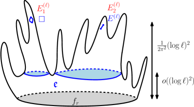
Figure 5: Illustration of the proof of Theorem 5.3: the map $\mathfrak{M}^{(\ell)}$ (or $\mathfrak{M}^{(\ell)}_{1}$) is represented as a cactus where the height corresponds to the distance to the root face $f_{r}$. The blue holes are the two holes of the explored region $\mathfrak{e}$. The target $2$-face $\square$ and the uniform random edge $E^{(\ell)}$ on $\mathfrak{M}^{(\ell)}_{1}$, in blue, correspond respectively to the random uniform edges $E_{1}^{(\ell)}$ and $E_{2}^{(\ell)}$ in $\mathfrak{M}^{(\ell)}$, in red.

Theorem 5.3.

If $\mathfrak{M}^{(\ell)}$ follows the law $\mathbb{P}^{(\ell)}$ and $E_{1}^{(\ell)},E_{2}^{(\ell)}$ are two uniform random edges of $\mathfrak{M}^{(\ell)}$, then

$${d^{\dagger}_{\mathrm{gr}}(E_{1}^{(\ell)},E_{2}^{(\ell)})\over(\log\ell)^{2}}\mathop{\longrightarrow}\limits_{\ell\to\infty}^{(\mathbb{P})}{1\over\pi^{2}}\ \text{ and }\ {d^{\dagger}_{\mathrm{fpp}}(E_{1}^{(\ell)},E_{2}^{(\ell)})\over\log\ell}\mathop{\longrightarrow}\limits_{\ell\to\infty}^{(\mathbb{P})}{2\over\pi^{2}p_{\bf q}}$$

The general idea of the proof is given in Figure 5. The key step is an intermediate result for the map $\mathfrak{M}^{(\ell)}_{1}$ of law $\mathbb{P}^{(\ell)}_{1}$.

Lemma 5.4.

If $\mathfrak{M}^{(\ell)}_{1}$ is a random map with target of law $\mathbb{P}^{(\ell)}_{1}$ and $E^{(\ell)}$ is a random uniform edge on $\mathfrak{M}^{(\ell)}_{1}$ (where the target $2$-face has been zipped and is considered as an edge), then

$$\frac{d^{\dagger}_{\mathrm{gr}}(\square,E^{(\ell)})-d^{\dagger}_{\mathrm{gr}}(f_{r},E^{(\ell)})}{(\log\ell)^{2}}\mathop{\longrightarrow}\limits_{\ell\to\infty}^{(\mathbb{P})}{1\over 2\pi^{2}}\ \text{ and }\ \frac{d^{\dagger}_{\mathrm{fpp}}(\square,E^{(\ell)})-d^{\dagger}_{\mathrm{fpp}}(f_{r},E^{(\ell)})}{\log\ell}\mathop{\longrightarrow}\limits_{\ell\to\infty}^{(\mathbb{P})}{1\over\pi^{2}p_{\bf q}}$$

Proof.

We consider the filled-in peeling exploration of $\mathfrak{M}^{(\ell)}_{1}$ using the algorithm $\mathcal{A}_{\mathrm{layers}}$ for the dual graph distance and the algorithm $\mathcal{A}_{\mathrm{uniform}}$ for the fpp distance. Let $n$ be the time at which during an event of type $G$, $\square$ and $E^{(\ell)}$ are in two distinct holes $\mathfrak{h}_{1}$ and $\mathfrak{h}_{2}$ (when it exists). By Lemma 5.2, we know that for $\varepsilon$ small, $n\leq\tau^{(\ell)}_{-1}-\varepsilon\ell$ with large probability. We also denote by $\mathfrak{e}$ the sub-map obtained after identifying the edges but before filling-in the hole containing $E^{(\ell)}$.

We work with the dual graph distance, and thus with the peeling by layers algorithm. We point out that a path from $\square$ to $E^{(\ell)}$ must go through $\mathfrak{e}$ (see Figure 5), so that

$$d^{\dagger}_{\mathrm{gr}}(\square,E^{(\ell)})\geq d^{\dagger}_{\mathrm{gr}}(\partial\mathfrak{e},\square)+d^{\dagger}_{\mathrm{gr}}(\partial\mathfrak{e},E^{(\ell)}).$$

But at time $n$, the perimeter $P_{1}(n)$ is larger than some constant times $\ell$ with large probability thanks to Proposition 2.4 since $n\leq\tau_{-1}-\varepsilon\ell$. Consequently, by Proposition 4.2, and since the map filling the hole $\mathfrak{h}_{1}$ has the law $\mathbb{P}^{(P_{1}(n))}_{1}$ conditionally on the exploration up to time $n$ by Proposition 3.1,

$$d^{\dagger}_{\mathrm{gr}}(\partial\mathfrak{e},\square)={(\log\ell)^{2}\over 2\pi^{2}}(1+o(1))\qquad\text{and}\qquad d^{\dagger}_{\mathrm{gr}}(f_{r},\square)={(\log\ell)^{2}\over 2\pi^{2}}(1+o(1))$$

in probability on the event that $n$ exists and $n\leq\tau_{-1}-\varepsilon\ell$. In particular, in probability and on the same event, $d^{\dagger}_{\mathrm{gr}}(f_{r},\partial\mathfrak{e})=o((\log\ell)^{2}).$ As a consequence, $d^{\dagger}_{\mathrm{gr}}(f_{r},E^{(\ell)})=d^{\dagger}_{\mathrm{gr}}(\partial\mathfrak{e},E^{(\ell)})+o((\log\ell)^{2})$. Thus, in probability,

$$d^{\dagger}_{\mathrm{gr}}(\square,E^{(\ell)})\geq{(\log\ell)^{2}\over 2\pi^{2}}(1+o(1))+d^{\dagger}_{\mathrm{gr}}(f_{r},E^{(\ell)}).$$

The converse inequality is a direct consequence of the triangle inequality and Proposition 4.2. For the fpp distance, the same reasoning holds using Proposition 4.1. ∎

Remark 5.5.

In the above proof, we saw that $d^{\dagger}_{\mathrm{gr}}(f_{r},\partial\mathfrak{e})=o((\log\ell)^{2})$ and $d^{\dagger}_{\mathrm{fpp}}(f_{r},\partial\mathfrak{e})=o(\log\ell)$. Nonetheless, it is easy to see that $d_{\mathrm{fpp}}^{\dagger}(f_{r},\partial\mathfrak{e})=O(1)$ in probability using Proposition 2.4 and Lemma 5.2. Moreover, we point out that Lemma 6.6, together with Lemma 5.2, enables to show that $d^{\dagger}_{\mathrm{gr}}(f_{r},\partial\mathfrak{e})=O(\log\ell)$ in probability.

Theorem 5.3 follows by a judicious application of Lemma 3.3:

Proof of Theorem 5.3.

For the dual graph distance, we apply Lemma 3.3 and Lemma 5.4 to the function $\varphi_{\ell}$ defined by

$$\forall\mathfrak{m}_{\square}\in\mathcal{M}^{(\ell)}_{1},\qquad\varphi_{\ell}(\mathfrak{m}_{\square})=\mathbb{E}\left(\left|\frac{d^{\dagger}_{\mathrm{gr}}(\square,E(\mathfrak{m}_{\square})-d^{\dagger}_{\mathrm{gr}}(f_{r},E(\mathfrak{m}_{\square}))}{(\log\ell)^{2}}-\frac{1}{2\pi^{2}}\right|\wedge 1\right),$$

where $E(\mathfrak{m}_{\square})$ is a random uniform edge on $\mathfrak{m}_{\square}$ (where the target $2$-face is considered as a single edge). As a result, we obtain that if $E_{1}^{(\ell)}$ and $E^{(\ell)}_{2}$ are two independent random uniform edges in $\mathfrak{M}^{(\ell)}$, then

$$\mathbb{E}\left(\left|\frac{d^{\dagger}_{\mathrm{gr}}(E_{1}^{(\ell)},E_{2}^{(\ell)})-d^{\dagger}_{\mathrm{gr}}(f_{r},E_{2}^{(\ell)})}{(\log\ell)^{2}}-\frac{1}{2\pi^{2}}\right|\wedge 1\right)\mathop{\longrightarrow}\limits_{\ell\to\infty}0.$$

The first convergence of the theorem then follows by applying once again Proposition 4.2. For the fpp distance, the function $\varphi_{\ell}$ is defined similarly but the expectation also involves the exponential weights defining the fpp distance. ∎

Using the same ideas as in the proof of Proposition 4.6 we also obtain the following result

Corollary 5.6.

If $\mathfrak{M}^{(\ell)}$ follows the law $\mathbb{P}^{(\ell)}$ and $V_{1},V_{2}$ are two uniform vertices of $\mathfrak{M}^{(\ell)}$, then

$${d^{\dagger}_{\mathrm{gr}}(V_{1},V_{2})\over(\log\ell)^{2}}\mathop{\longrightarrow}\limits_{\ell\to\infty}^{(\mathbb{P})}{1\over\pi^{2}}\ \text{ and }\ {d^{\dagger}_{\mathrm{fpp}}(V_{1},V_{2})\over\log\ell}\mathop{\longrightarrow}\limits_{\ell\to\infty}^{(\mathbb{P})}{2\over\pi^{2}p_{\bf q}}.$$

Proof.

We do the proof for the dual graph distance, the same ideas work for the fpp distance. We can work with $d_{\mathrm{gr}}^{\dagger}(\vec{E}_{1},\vec{E}_{2})$ where $\vec{E}_{1}$,$\vec{E}_{2}$ are i.i.d. oriented edges whose law is the same as the law of $\vec{E}$ in (4.4) since $d_{\mathrm{gr}}^{\dagger}(\vec{E}_{1},\vec{E}_{2})-\deg(V_{1}^{(\ell)})-\deg(V_{2}^{(\ell)})\leq d_{\mathrm{gr}}^{\dagger}(V_{1}^{(\ell)},V_{2}^{(\ell)})\leq d_{\mathrm{gr}}^{\dagger}(\vec{E}_{1},\vec{E}_{2})$ and since by Lemma 4.5 $\deg V^{(\ell)}_{1}$ and $\deg V^{(\ell)}_{2}$ are stochastically dominated by a random variable which does not depend on $\ell$. We then conclude by following the same lines as in the proof of Proposition 4.6 using Theorem 5.3. ∎

We finally prove Corollary 5.1 using the same ideas as in the proof of Theorem 1.1 in Subsection 4.3 and using Theorem 5.3.

6 Diameter of $\mathfrak{M}^{(\ell,\dagger)}$

The main purpose of this section is to give bounds on the diameter of $\mathfrak{M}^{(\ell,\dagger)}$ for the graph distance and for the fpp distance, proving Theorem 1.2. The upper bounds are achieved using a first moment method together with large deviations on the height of a uniform random edge, obtained using supermartingales. Two of these supermartingales (of Lemmas 6.2 and 6.9) are related to the martingale $(M_{n}^{(\ell)})_{n\geq 0}$ defined using the perimeter process $P_{\ell}$ under $\mathbb{P}^{(1)}_{\ell}$ as follows:

$$\forall n\geq 0,\qquad M_{n}^{(\ell)}=\frac{1}{h^{\downarrow}_{\ell}(P_{\ell}(n))}\prod_{j=0}^{n-1}\left(\frac{1}{\nu([-P_{\ell}(j)+1,\infty))+\nu(-P_{\ell}(j)-\ell)}\vee{\bf 1}_{P_{\ell}(j)=-\ell}\right).$$ (6.1)

This martingale is particularly well suited to the study of the distances on $3/2$-stable maps owing to the asymptotic behavior (1.3) of the step distribution $\nu$: intuitively, the above product can be approximated by the exponential of $\sum_{j=0}^{n-1}1/P_{\ell}(j)$ (times an appropriate constant) and can thus be related to the fpp and dual graph distances.

One notable fact is that our bounds show that the diameter under the fpp distance heavily depends on the tails of $\nu$, but also on the non-asymptotic behavior of $\nu$. Hence, even though the fpp diameter and the distance between uniform points are of the same order, the ratio does not converge to a universal constant. On the contrary, in the case of the dual graph distance, our upper bound for the diameter is universal, echoing the universal scaling limit of the height of a random uniform face in Theorem 1.1.

6.1 Upper bound of the diameter for the fpp distance

In this subsection, we upper bound the diameter of $\mathfrak{M}^{(\ell,\dagger)}$ for the first-passage percolation distance. Let $\gamma({\bf q})\coloneqq\min_{k,\ell\geq 1}k(\nu((-\infty,-k])-\nu(-\ell-k)))$, which is well defined thanks to (1.3). The proposition below implies the first upper bound of Theorem 1.2.

Proposition 6.1.

Let $\mathrm{Diam}_{\mathrm{fpp}}^{\dagger}(\mathfrak{M}^{(\ell)})$ be the diameter of $\mathfrak{M}^{(\ell,\dagger)}$ for the fpp distance. Then there exists a constant $C>0$ which does not depend on $\bf q$ such that with probability $1-o(1)$ when $\ell\to\infty$,

$$\frac{\mathrm{Diam}_{\mathrm{fpp}}^{\dagger}(\mathfrak{M}^{(\ell)})}{\log\ell}\leq C\left(1+\frac{1}{\gamma({\bf q})}\right).$$

So as to prove the above proposition, we introduce a first family of supermartingales associated to the perimeter process and related to the martingale (6.1):

Lemma 6.2.

Let $\lambda>0$. For all $\ell\geq 1,n\geq 0$, let

$$M^{\lambda,\ell}_{n}=\frac{1}{h^{\downarrow}_{\ell}(P_{\ell}(n))}\exp\left({\lambda\sum_{j=0}^{n-1}\frac{1}{P_{\ell}(j)}{\bf 1}_{P_{\ell}(j)>0}}\right).$$

If $\lambda<e^{-1}\gamma({\bf q})$, then for all $\ell\geq 1$, under $\mathbb{P}_{\ell}^{(1)}$, $(M_{n}^{\lambda,\ell})_{n\geq 0}$ is a supermartingale with respect to the filtration $(\mathcal{F}_{n})_{n\geq 0}$ associated to the peeling exploration.

Proof.

If $\lambda<e^{-1}\gamma({\bf q})$, then for all $\ell\geq 1,n\geq 0$,

$$\mathbb{E}_{\ell}^{(1)}\left(\left.M_{n+1}^{\lambda,\ell}\right|\mathcal{F}_{n}\right) =\sum_{\begin{subarray}{c}k>-P_{\ell}(n)\\ \text{ or }k=-P_{\ell}(n)-\ell\end{subarray}}\frac{1}{h^{\downarrow}_{\ell}(P_{\ell}(n)+k)}\exp\left({\lambda\sum_{j=0}^{n}\frac{1}{P_{\ell}(j)}{\bf 1}_{P_{\ell}(j)>0}}\right)\frac{h^{\downarrow}_{\ell}(P_{\ell}(n)+k)}{h^{\downarrow}_{\ell}(P_{\ell}(n))}\nu(k)$$

$$=M_{n}^{\lambda,\ell}e^{\lambda\frac{1}{P_{\ell}(n)}{\bf 1}_{P_{\ell}(n)>0}}\left(\left(\sum_{k>-P_{\ell}(n)}\nu(k)\right)+\nu(-P_{\ell}(n)-\ell)\right)$$

$$\leq M_{n}^{\lambda,\ell},$$

thanks to the definition of $\gamma({\bf q})$. ∎

The above supermartingales lead to a large deviation inequality for the distance from the root to a uniform random edge.

Corollary 6.3.

Let $c>0$. Let $E$ be a uniform random edge of $\mathfrak{M}^{(\ell)}$. If $K>0$ is large enough, then

$$\mathbb{P}\left(d_{\mathrm{fpp}}^{\dagger}(f_{r},E)\geq K\log\ell\right)=O(\ell^{-c})\text{ when }\ell\to\infty.$$

One can choose $K=C^{\prime}(1+c)(1+1/\gamma({\bf q}))$, where $C^{\prime}$ is large enough and does not depend on $\bf q$, $c$.

Proof.

Let $c>0$. First of all, since the distance to an edge is smaller than the distance to the $2$-face obtained by unzipping the edge, and by (3.4),

$$\mathbb{P}\left(d_{\mathrm{fpp}}^{\dagger}(f_{r},E)\geq K\log\ell\right) \leq\frac{W_{1}^{(\ell)}}{W^{(\ell)}}\mathbb{E}_{1}^{(\ell)}\left(\frac{1}{\#\mathrm{Edges}(\mathfrak{m}_{\square})-1}{\bf 1}_{d_{\mathrm{fpp}}^{\dagger}(f_{r},\square)\geq K\log\ell}\right)$$

$$\leq\frac{W_{1}^{(\ell)}}{W^{(\ell)}}\mathbb{P}_{1}^{(\ell)}\left(d_{\mathrm{fpp}}^{\dagger}(f_{r},\square)\geq K\log\ell\right).$$

But, owing to (3.3), we know that $W_{1}^{(\ell)}/W^{(\ell)}$ is a $O(\ell^{3/2})$, so that it is enough to prove the analogous statement for $\mathbb{P}_{1}^{(\ell)}(d_{\mathrm{fpp}}^{\dagger}(f_{r},\square)\geq K\log\ell)$. Moreover, recalling (4.1), one can see that it suffices to show that there exists $K^{\prime}>0$ such that

$$\mathbb{P}^{(1)}_{\ell}\left(\sum_{k=0}^{\tau_{-\ell}-1}{1\over P_{\ell}(k)}\geq K^{\prime}\log\ell\right)=O(\ell^{-c})\text{ when }\ell\to\infty.$$ (6.2)

Indeed, if we assume (6.2), then by conditioning on the perimeter process and applying Bernstein’s inequality (the version we use comes from Corollary 2.10 of [25]), we get that there exists a constant $C>0$ such that for all $\ell\geq 1$ and for all $t>0$,

$$\mathbb{P}^{(1)}_{\ell}\left(\left.\left|\sum_{k=0}^{\tau_{-\ell}-1}\frac{\mathcal{E}_{k}-1}{P_{\ell}(k)}\right|>t\log\ell\right|P_{\ell}\right) \leq 2\exp\left(-C\min\left(\frac{t^{2}(\log\ell)^{2}}{\sum_{k=0}^{\tau_{-\ell}-1}\frac{1}{P_{\ell}(k)^{2}}},\frac{t\log\ell}{\max_{0\leq k\leq\tau_{-\ell}-1}\frac{1}{P_{\ell}(k)}}\right)\right)$$

$$\leq 2\exp\left(-C\min\left(\frac{t^{2}(\log\ell)^{2}}{\sum_{k=0}^{\tau_{-\ell}-1}\frac{1}{P_{\ell}(k)}},t\log\ell\right)\right)$$

$$\leq 2\ell^{-(\frac{Ct^{2}}{K^{\prime}}\wedge Ct)}\text{ with probability at least }1-O(\ell^{-c}).$$

One can then conclude by choosing $t>0$ such that $\frac{Ct^{2}}{K^{\prime}}\wedge Ct\geq c$ and by taking $K=\frac{K^{\prime}+t}{2}$.

Now, let us prove (6.2). Let $\lambda>0$ small enough so that for all $\ell\geq 1$, $M^{\lambda,\ell}$ is a supermartingale (given by Lemma 6.2). Then, using Markov’s inequality and Fatou’s lemma,

$$\mathbb{P}^{(1)}_{\ell}\left(\sum_{k=0}^{\tau_{-\ell}-1}{1\over P_{\ell}(k)}\geq K^{\prime}\log\ell\right) \leq\ell^{-\lambda K^{\prime}}\mathbb{E}^{(1)}_{\ell}e^{\lambda\sum_{k=0}^{\tau_{-\ell}-1}\frac{1}{P_{\ell}(k)}}$$

$$=\ell^{-\lambda K^{\prime}}\mathbb{E}^{(1)}_{\ell}M^{\lambda,\ell}_{\tau_{-\ell}}$$

$$\leq\ell^{-\lambda K^{\prime}}\mathbb{E}^{(1)}_{\ell}M^{\lambda,\ell}_{0}=\ell^{-\lambda K^{\prime}}\frac{1}{h^{\downarrow}_{\ell}(1)}=O(\ell^{3/2-\lambda K^{\prime}})=O(\ell^{-c})$$

for $K^{\prime}\geq(c+3/2)/\lambda$. ∎

Proof of Proposition 6.1.

To begin with, since the diameter is upper bounded by twice the maximal distance to the root face, it suffices to show that there exists $K>0$ such that

$$\mathbb{P}\left(\exists e\in\mathrm{Edges}(\mathfrak{M}^{(\ell)}),\ d_{\mathrm{fpp}}^{\dagger}(f_{r},e)\geq K\log\ell\right)\mathop{\longrightarrow}\limits_{\ell\to\infty}0,$$

using also that for all $f\in\mathrm{Faces}(\mathfrak{M}^{(\ell)})$, if $e$ is an edge surrounding $f$, then $d_{\mathrm{fpp}}^{\dagger}(f_{r},f)\leq d_{\mathrm{fpp}}^{\dagger}(f_{r},e)+\mathcal{E}$, where $\mathcal{E}$ is an exponential random variable of parameter $1$.

Then we distinguish whether the number of edges is too large or not: let $\varepsilon>0$.

$$\mathbb{P} \left(\exists e\in\mathrm{Edges}(\mathfrak{M}^{(\ell)}),\ d_{\mathrm{fpp}}^{\dagger}(f_{r},e)\geq K\log\ell\right)$$

$$\leq \enskip\mathbb{E}\left(\#\left\{e\in\mathrm{Edges}(\mathfrak{M}^{(\ell)});\ d_{\mathrm{fpp}}^{\dagger}(f_{r},e)\geq K\log\ell\right\}{\bf 1}_{\#\mathrm{Edges}(\mathfrak{M}^{(\ell)})\leq\frac{2b_{\bf q}}{\varepsilon}\ell^{3/2}}\right)$$

$$+\mathbb{P}\left(\#\mathrm{Edges}(\mathfrak{M}^{(\ell)})\geq\frac{2b_{\bf q}}{\varepsilon}\ell^{3/2}\right)$$

and the last term is smaller than $\varepsilon$ for $\ell$ large enough by (3.3). Henceforth we focus on the first term. Conditionally on $\mathfrak{M}^{(\ell)}$, let $E$ be a uniform random edge of $\mathfrak{M}^{(\ell)}$.

$$\mathbb{E} \left(\#\left\{e\in\mathrm{Edges}(\mathfrak{M}^{(\ell)});\ d_{\mathrm{fpp}}^{\dagger}(f_{r},e)\geq K\log\ell\right\}{\bf 1}_{\#\mathrm{Edges}(\mathfrak{M}^{(\ell)})\leq\frac{2b_{\bf q}}{\varepsilon}\ell^{3/2}}\right)$$

$$\leq\mathbb{E}\left(\frac{2b_{\bf q}}{\varepsilon}\ell^{3/2}\mathbb{P}(d_{\mathrm{fpp}}^{\dagger}(f_{r},E)\geq K\log\ell|\mathfrak{M}^{(\ell)})\right)$$

$$=\frac{2b_{\bf q}}{\varepsilon}\ell^{3/2}\mathbb{P}(d_{\mathrm{fpp}}^{\dagger}(f_{r},E)\geq K\log\ell).$$

The expression on the last line tends to zero when $\ell\to\infty$ if $K$ is chosen large enough according to Corollary 6.3. ∎

6.2 Lower bound for the diameter for the fpp distance

A lower bound for the diameter is already provided by Corollary 5.1. Nevertheless, this lower bound only depends on the tail behavior of $\nu$. Actually, in the case of the fpp distance, the diameter depends heavily on $\nu$. Let us show for instance the influence of $q_{1}$, or equivalently $\nu(0)$, on the asymptotic behavior of the diameter, which implies in particular the first lower bound of Theorem 1.2, hence ending the proof of that theorem.

Proposition 6.4.

For all $\delta>0$, with probability $1-o(1)$ as $\ell\to\infty$,

$$\frac{\mathrm{diam}_{\mathrm{fpp}}^{\dagger}(\mathfrak{M}^{(\ell)})}{\log\ell}\geq\frac{3}{4(1-q_{1}^{2})}-\delta.$$

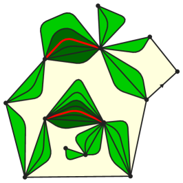
Figure 6: On the left, the map $\mathfrak{M}^{(\ell)}$ with two random edges $E_{1}$ and $E_{2}$ in red. The $2$-faces are in green and form “watermelons” and $E_{1}$ and $E_{2}$ are in the middle of their watermelons. The largest fpp-balls around $E_{1}$ and $E_{2}$ made of $2$-faces only are in dark green. On the right the map $\widetilde{\mathfrak{M}}^{(\ell)}$ obtained from $\mathfrak{M}^{(\ell)}$ by deleting the $2$-faces. The blue edges are the two random uniform edges $\tilde{E}_{1}$ and $\tilde{E}_{2}$ that correspond to the two watermelons containing $E_{1}$ and $E_{2}$.

Proof.

Let us prove that result with a second moment method. If $e$ is an edge of $\mathfrak{M}^{(\ell)}$, let $R(e)$ denote the radius of the largest fpp-ball centred at $e$ only constituted of faces of degree $2$. Notice that this fpp-ball is included in the maximal sub-map made of $2$-faces and edges which have the same endpoints as $e$, which is called the “watermelon” containing $e$ (see Figure 6).

By Proposition 11.10 of [13], we know that the map $\widetilde{\mathfrak{M}}^{(\ell)}$ obtained from $\mathfrak{M}^{(\ell)}$ by replacing each watermelon by one edge (see Figure 6) is a $\tilde{\bf q}$-Boltzmann map of perimeter $2\ell$, where the weight sequence $\tilde{\bf q}$ is defined by

$$\left\{\begin{array}[]{lc}\tilde{q}_{1}=0&\\ \tilde{q}_{k}=q_{k}/(1-q_{1})^{k}&\text{for }k\geq 2.\end{array}\right.$$

Moreover, conditionally on $\widetilde{\mathfrak{M}}^{(\ell)}$, the map ${\mathfrak{M}}^{(\ell)}$ is obtained by adding independently a geometric number of $2$-faces on each edge of $\widetilde{\mathfrak{M}}^{(\ell)}$, with parameter $q_{1}$. We denote by $M(\tilde{e})$ the number of edges of the watermelon corresponding to an edge $\tilde{e}$ of $\widetilde{\mathfrak{M}}^{(\ell)}$ so that conditionally on $\widetilde{\mathfrak{M}}^{(\ell)}$, the random variables $M(\tilde{e})-1$ are i.i.d. geometric of parameter $q_{1}$. By the paragraph just above Proposition 11.10 in [13] we also know that $c_{\bf q}=c_{\tilde{\bf q}}/(1-q_{1})$ and that $\tilde{\bf q}$ is again a critical weight sequence of type $2$.

If $\tilde{E}$ is a random uniform edge in $\widetilde{\mathfrak{M}}^{(\ell)}$ and $E$ is the edge in the middle of the watermelon corresponding to $\tilde{E}$ (and if the watermelon has an even number of edges, we choose $E$ uniformly among the two edges in the middle), then, conditionally on $\widetilde{\mathfrak{M}}^{(\ell)}$ and on $\tilde{E}$, the random variable $M(\widetilde{E})$ is geometric of parameter $q_{1}$ starting at one. Hence, $R(E)$ is lower-bounded by a sum of $\lfloor M(E)/2\rfloor-1$ exponential random variables of parameter $2$ (i.e. of expectation $1/2$). As a consequence, for all $t\geq 0$,

$$\mathbb{P}\left(R(E)\geq t\left|\widetilde{\mathfrak{M}}^{(\ell)},\tilde{E}\right.\right)\geq\mathbb{P}\left(\left.\sum_{i=1}^{\lfloor M(\tilde{E})/2\rfloor-1}\frac{\mathcal{E}_{i}}{2}\geq t\right|\widetilde{\mathfrak{M}}^{(\ell)},\tilde{E}\right),$$

where the $\mathcal{E}_{i}$’s are i.i.d. exponential random variables of parameter $1$ which are independent from $\widetilde{\mathfrak{M}}^{(\ell)}$ and $M(\tilde{E})$. But one can lower-bound

$$\mathbb{P}\left(\left.\sum_{i=1}^{\lfloor M(\tilde{E})/2\rfloor-1}\frac{\mathcal{E}_{i}}{2}\geq t\right|\widetilde{\mathfrak{M}}^{(\ell)},\tilde{E}\right) =\sum_{k=4}^{\infty}q_{1}^{k-1}(1-q_{1})\int_{2t}^{\infty}\frac{x^{\lfloor k/2\rfloor-2}e^{-x}}{(\lfloor k/2\rfloor-2)!}dx$$

$$\geq q_{1}^{5}(1-q_{1})\int_{2t}^{\infty}\sum_{k=4}^{\infty}(q_{1}^{2})^{\lfloor k/2\rfloor-2}\frac{x^{\lfloor k/2\rfloor-2}e^{-x}}{(\lfloor k/2\rfloor-2)!}dx$$

$$=2q_{1}^{5}(1-q_{1})\int_{2t}^{\infty}e^{(q_{1}^{2}-1)x}dx$$

$$=\frac{2q_{1}^{5}}{1+q_{1}}e^{-2(1-q_{1}^{2})t}.$$

Henceforth, let $\tilde{E}_{1},\ldots,\tilde{E}_{\lfloor\ell^{3/2}\rfloor}$ be independent random uniform edges of $\widetilde{\mathfrak{M}}^{(\ell)}$ (conditionally on $\widetilde{\mathfrak{M}}^{(\ell)}$). For all $1\leq i\leq\lfloor\ell^{3/2}\rfloor$, we write $E_{i}$ the edge of $\mathfrak{M}^{(\ell)}$ in the middle of the watermelon corresponding to $\tilde{E}_{i}$ (chosen uniformly at random between the two edges in the middle if the watermelon has an even number of edges). We again write $R(E_{i})$ the radius of the largest fpp-ball centred at $E_{i}$ containing only $2$-faces. For conciseness we drop the $\lfloor\cdot\rfloor$. If $t>0$, then by the second moment method,

$$\mathbb{P} \left(\left.\exists i\leq\ell^{3/2},R(E_{i})\geq t\log\ell\right|\widetilde{\mathfrak{M}}^{(\ell)}\right)$$

$$\geq\frac{\mathbb{E}(\#\left\{i\in[\![1,\ell^{3/2}]\!],R(E_{i})\geq t\log\ell\right\}|\widetilde{\mathfrak{M}}^{(\ell)})^{2}}{\mathbb{E}((\#\left\{i\in[\![1,\ell^{3/2}]\!],R(E_{i})\geq t\log\ell\right\})^{2}|\widetilde{\mathfrak{M}}^{(\ell)})}$$

$$=\frac{\ell^{3}\mathbb{P}(R(E)\geq t\log\ell|\widetilde{\mathfrak{M}}^{(\ell)})^{2}}{\ell^{3/2}\mathbb{P}(R(E)\geq t\log\ell|\widetilde{\mathfrak{M}}^{(\ell)})+\ell^{3/2}(\ell^{3/2}-1)\mathbb{P}(R(E_{1}),R(E_{2})\geq t\log\ell|\widetilde{\mathfrak{M}}^{(\ell)})}$$

Now, one can distinguish whether $\tilde{E}_{1}=\tilde{E}_{2}$ or not. Then, in probability as $\ell\to\infty$,

$$\mathbb{P} (R(E_{1}),R(E_{2})\geq t\log\ell|\widetilde{\mathfrak{M}}^{(\ell)})$$

$$\leq\mathbb{P}(\tilde{E}_{1}=\tilde{E}_{2}\text{ and }R(E_{1})\geq t\log\ell|\widetilde{\mathfrak{M}}^{(\ell)})+\mathbb{P}(\tilde{E}_{1}\neq\tilde{E}_{2}\text{ and }R(E_{1}),R(E_{2})\geq t\log\ell|\widetilde{\mathfrak{M}}^{(\ell)})$$

$$=\frac{1}{\#\mathrm{Edges}(\widetilde{\mathfrak{M}}^{(\ell)})}\mathbb{P}(R(E)\geq t\log\ell|\widetilde{\mathfrak{M}}^{(\ell)})+\frac{\#\mathrm{Edges}(\widetilde{\mathfrak{M}}^{(\ell)})-1}{\#\mathrm{Edges}(\widetilde{\mathfrak{M}}^{(\ell)})}\mathbb{P}(R(E_{1}),R(E_{2})\geq t\log\ell|\tilde{E}_{1}\neq\tilde{E}_{2},\widetilde{\mathfrak{M}}^{(\ell)})$$

$$=O(\ell^{-3/2})\mathbb{P}(R(E)\geq t\log\ell|\widetilde{\mathfrak{M}}^{(\ell)})+\mathbb{P}(R(E)\geq t\log\ell|\widetilde{\mathfrak{M}}^{(\ell)})^{2},$$

where the last line is due to the convergence in distribution of $\#\mathrm{Edges}(\widetilde{\mathfrak{M}}^{(\ell)})\ell^{-3/2}$ as $\ell\to\infty$, see e.g. Proposition 10.4 in [13].

By taking $t<3/(4(1-q_{1}^{2}))$ we ensure that $\ell^{3/2}\mathbb{P}(R(E)\geq t\log\ell|\widetilde{\mathfrak{M}}^{(\ell)})\to\infty$ in probability as $\ell\to\infty$, hence

$$\mathbb{P}\left(\left.\exists i\leq\ell^{3/2},R(E_{i})\geq t\log\ell\right|\widetilde{\mathfrak{M}}^{(\ell)}\right)\mathop{\longrightarrow}\limits_{\ell\to\infty}^{(\mathbb{P})}1.$$

This entails what we wanted to show. ∎

6.3 Upper bound of the diameter for the graph distance

We next upper bound the diameter of $\mathfrak{M}^{(\ell,\dagger)}$ for the graph distance. The proposition below implies the second upper bound of Theorem 1.2. Unlike the case of the fpp distance, the upper bound for the graph distance is universal (i.e. it does not depend on $\bf q$).

Proposition 6.5.

Let $\mathrm{Diam}_{\mathrm{gr}}^{\dagger}(\mathfrak{M}^{(\ell)})$ be the diameter of $\mathfrak{M}^{(\ell,\dagger)}$ for the graph distance. Then for all $\delta>0$, with probability $1-o(1)$ when $\ell\to\infty$,

$$\frac{\mathrm{Diam}_{\mathrm{gr}}^{\dagger}(\mathfrak{M}^{(\ell)})}{(\log\ell)^{2}}\leq 18+\delta.$$

To prove this result, we will need to use the height process $H_{\ell}$ during the peeling by layers exploration, together with the interpolated height process. Let us first recall the definition of the interpolated height process from [11]. At time $n$ of the exploration, let $D_{n}$ be the number of edges in the boundary $\partial\overline{\mathfrak{e}}_{n}$ that are at height $H_{\ell}(n)$, so that the other $2P_{\ell}(n)-D_{n}$ edges are at height $H_{\ell}(n)+1$. If $f:[0,1]\to[0,1]$ is a non-increasing function, the interpolated height process $H^{f}_{\ell}(n)$ under $\mathbb{P}^{(1)}_{\ell}$ and its increment at time $n<\tau_{-\ell}$ are defined by

$$H_{\ell}^{f}(n)\coloneqq H_{\ell}(n)+f(D_{n}/2P_{n})\qquad\text{and}\qquad\Delta H_{\ell}^{f}(n)\coloneqq H_{\ell}^{f}(n+1)-H_{\ell}^{f}(n),$$

where by convention, we set $H^{f}_{\ell}(n)=H^{f}_{\ell}(\tau_{-\ell}-1)$ for $n\geq\tau_{-\ell}$. The next lemma is an analogue of Lemma 6 from [11], bounding from above the mean increase of the interpolated height.

Lemma 6.6.

Let $0<\varepsilon<1$. If $f:[0,1]\to[0,1]$ is twice continuously differentiable with $f(0)=1,f(1)=0,f^{\prime}(0)=f^{\prime}(1)=f^{\prime\prime}(0)=f^{\prime\prime}(1)=0$ and $0\leq-f^{\prime}(x)\leq 1+\varepsilon$ for all $x\in[0,1]$, then there exist $C(\varepsilon,{\bf q}),C^{\prime}(\varepsilon,{\bf q})>0$ such that for all $\ell_{0}\geq 1,\ell\geq 1,n\geq 0$,

$$\mathbb{E}^{(\ell_{0})}_{\ell}\left(\left.\Delta H_{\ell}^{f}(n)\right|\mathcal{F}_{n}\right)\leq\frac{(1+3\varepsilon)^{2}}{1-\varepsilon}\frac{p_{\bf q}}{2}\frac{\log(P_{\ell}(n))+C(\varepsilon,{\bf q})}{P_{\ell}(n)}\enskip\text{and}\enskip\mathbb{E}^{(\ell_{0})}_{\ell}\left(\left.\left(\Delta H_{\ell}^{f}(n)\right)^{2}\right|\mathcal{F}_{n}\right)\leq\frac{C^{\prime}(\varepsilon,{\bf q})}{P_{\ell}(n)},$$

where $(\mathcal{F}_{n})_{n\geq 0}$ is the filtration associated to the exploration process.

Proof.

The proof is essentially the same as the proof of Lemma 6 of [11], but a little more complex. Indeed, the same terms appear except that they are multiplied by a factor $(p+\ell)/(p+k+\ell)$. Let us detail the proof.

We extend $f$ to $\mathbb{R}$ by setting $f(x)=1$ for $x\leq 0$ and $f(x)=0$ for all $x\geq 1$. As in [11], by the Markov property of the exploration (Proposition 3.1), we claim that $(H_{\ell}(n),P_{\ell}(n),D_{n})_{n\geq 0}$ is a Markov chain and that if $p\geq 1$ and $1\leq d\leq 2p$, then

$$\mathbb{E}^{(\ell_{0})}_{\ell} \left(\left.\Delta H_{\ell}^{f}(n)\right|P_{\ell}(n)=p,D_{n}=d\right)$$ (6.3)

$$= \sum_{k=0}^{\infty}\nu(k)\frac{p+\ell}{p+k+\ell}\frac{h^{\uparrow}(p+k)}{h^{\uparrow}(p)}\left[f\left(\frac{d-1}{2p+2k}\right)-f\left(\frac{d}{2p}\right)\right]$$ (6.4)

$$+\sum_{k=1}^{p-1}\frac{\nu(-k)}{2}\frac{p+\ell}{p-k+\ell}\frac{h^{\uparrow}(p-k)}{h^{\uparrow}(p)}\left[f\left(\frac{d-2k}{2p-2k}\right)-f\left(\frac{d}{2p}\right)\right]$$ (6.5)

$$+\sum_{k=1}^{p-1}\frac{\nu(-k)}{2}\frac{p+\ell}{p-k+\ell}\frac{h^{\uparrow}(p-k)}{h^{\uparrow}(p)}\left[f\left(\frac{d-1}{2p-2k}\right)-f\left(\frac{d}{2p}\right)\right].$$ (6.6)

Indeed, if $d=1$, then either $\Delta H_{\ell}(n)=1$ and $D_{n+1}=2P_{\ell}(n+1)$, and therefore $\Delta H_{\ell}^{f}(n)=1-f(1/(2p))$, with probability $\sum_{k=-p+1}^{\infty}\nu(k)(h^{\downarrow}_{\ell}(p+k)/h^{\downarrow}_{\ell}(p))$; or $\tau_{-\ell}=n+1$ and in that case $\Delta H_{\ell}^{f}(n)=0$, with probability $\nu(-p-\ell)/{h^{\downarrow}_{\ell}(p)}$. This agrees with the sums since $f(x)=1$ for $x\leq 0$ (and by using the definition of $h^{\uparrow}$ and $h^{\downarrow}_{\ell}$ in (2.1)). Now, in the case $d\geq 2$, if an event $C_{k+1}$ happens, then $P_{\ell}(n+1)=p+k$ and $D_{n+1}=d-1$, hence the first line (6.4) (again using (2.1)). If an event $G_{\square,k-1}$ happens for $1\leq k\leq p-1$, i.e. if the peeled edge is identified with an edge on its right, then $P_{\ell}(n+1)=P_{\ell}(n)-k$ and either $D_{n+1}=d-2k$ and $\Delta H_{\ell}(n)=0$, or $D_{n+1}=2P_{\ell}(n+1)$ and $\Delta H_{\ell}(n)=1$, depending on the sign of $d-2k$. These two cases are taken into account in the second line (6.5) since $f(x)=1$ for all $x\leq 0$. If an event $G_{k-1,\square}$ happens for some $1\leq k\leq p-1$, i.e. if the peeled edge is identified with an edge on its left, then again $P_{\ell}(n+1)=P_{\ell}(n)-k$ but $\Delta H_{\ell}(n)=0$ and either $D_{n+1}=d-1$ or $D_{n+1}=2P_{\ell}(n+1)$, depending on which is the smallest. Both situations are incorporated by the last line (6.6). Finally, if the event $C_{\ell}^{\mathrm{stop}}$ happens, then $\Delta H_{\ell}^{f}(n)=0$ by definition of the interpolated height process.

To deal with these three sums, we will use the notation $y=d/(2p)\in(0,1]$. Let $c>0$ given by Taylor’s theorem such that $|f(x)-f(y)-f^{\prime}(y)(x-y)|\leq c(x-y)^{2}$ for all $x\in\mathbb{R}$. We will also rely on the inequality

$$\forall k>-p,\qquad\sqrt{1+k/p}(1-1/p)\leq\frac{h^{\uparrow}(p+k)}{h^{\uparrow}(p)}\leq\sqrt{1+k/p}(1+1/p).$$

Let $N>0$ such that $1-\varepsilon<k^{2}\nu(-k)/p_{\bf q}<1+\varepsilon$ and $1-\varepsilon<k\nu([k,\infty))/p_{\bf q}<1+\varepsilon$ for all $k\geq N$, given by (1.3). From the mean value inequality applied to $f$, the first $N$ terms in each sum contribute $O(p^{-1})$ uniformly in $d,\ell$, so it suffices to bound the sums restricted to $|k|\geq N$. Since $(p+\ell)/(p+k+\ell)\leq 1$, the aforementioned inequalities, the first sum from $N$ to $\infty$, which only contains positive terms, is smaller than

$$\sum_{k=N}^{\infty}\nu(k)\sqrt{1+k/p}(1+1/p)\left[|f^{\prime}(y)|\frac{1+yk}{p+k}+c\left(\frac{1+k}{p+k}\right)^{2}\right]$$

where we used that

$$\frac{d}{2p}-\frac{d-1}{2p+2k}\leq\frac{1+yk}{p+k}\leq\frac{1+k}{p+k}.$$

Thus, by summation by parts, using that $1-\varepsilon<k\nu([k,\infty))/p_{\bf q}<1+\varepsilon$ for all $k\geq N$, and then recognizing a Riemann sum, the first sum (6.4) is upper bounded by

$$(1+\varepsilon)p_{\bf q}y\frac{1}{p}\int_{(N-1)/p}^{\infty}\frac{dx}{x\sqrt{1+x}}+O(p^{-1})\leq(1+\varepsilon)^{2}p_{\bf q}y\frac{\log p}{p}+O(p^{-1}),$$ (6.7)

where the $O(p^{-1})$ is uniform in $d$ and $\ell$. For the second sum (6.5), which again has only positive terms, we distinguish whether $k\leq\varepsilon p$ or $k>\varepsilon p$. If $k\leq\varepsilon p$, $(p+\ell)/(p-k+\ell)\leq 1/(1-\varepsilon)$, so that applying the inequalities and the fact that $1-\varepsilon<k^{2}\nu(-k)/p_{\bf q}<1+\varepsilon$ for all $k\geq N$ gives us that

$$\sum_{k=N}^{\varepsilon p}\frac{\nu(-k)}{2}\frac{p+\ell}{p-k+\ell} \frac{h^{\uparrow}(p-k)}{h^{\uparrow}(p)}\left[f\left(\frac{d-2k}{2p-2k}\right)-f\left(\frac{d}{2p}\right)\right]$$

$$\leq \sum_{k=N}^{\varepsilon p}\frac{1+\varepsilon}{1-\varepsilon}\frac{p_{\bf q}}{2k^{2}}(1+1/p)\sqrt{1-k/p}\left[|f^{\prime}(y)|(1-y)\frac{k}{p}\frac{1}{1-\frac{k}{p}}+c\left(\frac{k}{p}\frac{1}{1-\frac{k}{p}}\right)^{2}\right],$$

where we used that

$$\frac{d}{2p}-\frac{d-2k}{2p-2k}=(1-y)\frac{k}{p}\frac{1}{1-\frac{k}{p}}\leq\frac{k}{p}\frac{1}{1-\frac{k}{p}}.$$

Hence, by recognizing a Riemann sum, we can upper bound the sum for the $k\leq\varepsilon p$ by

$$\frac{1+\varepsilon}{1-\varepsilon}p_{\bf q}\frac{1-y}{2}|f^{\prime}(y)|\frac{1}{p}\int_{(N-1)/p}^{\varepsilon+1/p}\frac{1}{x\sqrt{1-x}}dx+O(p^{-1})\leq\frac{1+\varepsilon}{1-\varepsilon}p_{\bf q}\frac{1-y}{2}|f^{\prime}(y)|\frac{\log p}{p}+O(p^{-1}).$$

If $\varepsilon p\leq k\leq p-1$, we have

$$1\leq\frac{p+\ell}{p-k+\ell}\leq\frac{p}{p-k}$$

and

$$\frac{\nu(-k)}{2}\frac{h^{\uparrow}(p-k)}{h^{\uparrow}(p)}\left[f\left(\frac{d-2k}{2p-2k}\right)-f\left(\frac{d}{2p}\right)\right]\leq\nu(-k)\frac{h^{\uparrow}(p-k)}{h^{\uparrow}(p)}\leq\sqrt{(p-k)/p}O(p^{-2}).$$

So, using a Riemann sum, the sum for $k\geq\varepsilon p$ is upper bounded by $O(p^{-1})$. Therefore, the second sum (6.5) is bounded by

$$\frac{1+\varepsilon}{1-\varepsilon}p_{\bf q}\frac{1-y}{2}|f^{\prime}(y)|\frac{\log p}{p}+O(p^{-1}).$$ (6.8)

For the last sum (6.6), we first focus on the positive terms, i.e. those such that $kd\leq p$. If $d\geq 2$, then this entails that $(p+\ell)/(p-k+\ell)\leq 2$. Moreover, for all $1\leq k\leq p-1$,

$$\frac{d}{2p}-\frac{d-1}{2p-2k}\leq\frac{1}{2p},$$

so that the sum of the positive terms is a $O(p^{-1})$. If $d=1$, then by Taylor’s theorem $f(0)-f(1/(2p))=O(p^{-2})$, so that the sum of the positive terms is a $O(p^{-2})$. In these two cases, the sum of the positive terms of (6.6) is upper bounded by a $O(p^{-1})$. In the case $0<y<\varepsilon$, the upper bounds for the positive terms already enable to conclude since by summing (6.7), (6.8) and the $O(p^{-1})$, we obtain the uniform bound

$$\frac{(1+\varepsilon)^{3}}{1-\varepsilon}\frac{p_{\bf q}}{2}\frac{\log p}{p}+O(p^{-1})\leq\frac{(1+3\varepsilon)^{2}}{1-\varepsilon}\frac{p_{\bf q}}{2}\frac{\log p}{p}+O(p^{-1}).$$

In the case $y\geq\varepsilon$, we assume that we have chosen $N>1/\varepsilon$, so that $N\geq 2p/d$ and thus all the terms of (6.6) for $N\leq k\leq\varepsilon p$ are negative. Using that $(p+\ell)/(p-k+\ell)\geq 1$, the sum of the negative terms of (6.6) with $N\leq k\leq\varepsilon p$ can be upper bounded by

$$-\frac{1-\varepsilon}{2}\sum_{k=N}^{\varepsilon p}\frac{p_{\bf q}}{k^{2}}(1-1/p)\sqrt{1-k/p}\left[|f^{\prime}(y)|\left(y\frac{k}{p}-\frac{1}{2p}\right)-c(2k/p)^{2}\right],$$

where we used that

$$\frac{d-1}{2p-2k}-\frac{d}{2p}\geq\frac{dk-p}{2p^{2}}=y\frac{k}{p}-\frac{1}{2p}\qquad\text{and}\qquad\left|\frac{d}{2p}-\frac{d-1}{2p-2k}\right|\leq\frac{k}{(1-\varepsilon)p}.$$

Therefore, using again a Riemann sum, the sum (6.6) is upper bounded by

$$-(1-\varepsilon)p_{\bf q}\frac{y}{2}|f^{\prime}(y)|\frac{\log p}{p}+O(p^{-1}).$$ (6.9)

Finally, summing the upper bounds (6.7), (6.8), (6.9) and the $O(p^{-1})$, one recovers the desired result in the case $\varepsilon\leq y\leq 1$ as well for $\mathbb{E}^{(\ell_{0})}_{\ell}\left(\left.\Delta H_{\ell}^{f}(n)\right|\mathcal{F}_{n}\right)$. For the expectation of the square, one can perform the same computation with the three sums (6.4), (6.5), (6.6), except that the expressions into brackets are squared. One can check using the same ideas that each sum is a $O(p^{-1})$ (uniformly in $d,\ell$), hence the second upper bound. ∎

We will rely on a direct consequence of Lemma 6.6.

Corollary 6.7.

For all $\varepsilon\in(0,1)$, there exists $\lambda(\varepsilon)>0$ (which does not depend on $\bf q$) and $C(\varepsilon,{\bf q})>0$ such that for all $0<\lambda<\lambda(\varepsilon)$, for all $\ell\geq 1$ and $n\geq 0$,

$$\mathbb{E}^{(1)}_{\ell}\left(\left.e^{\lambda\Delta H_{\ell}^{f}(n)}\right|\mathcal{F}_{n}\right)\leq 1+\lambda\left(\frac{(1+3\varepsilon)^{2}}{1-\varepsilon}\frac{p_{\bf q}}{2}{\log(P_{\ell}(n))\over P_{\ell}(n)}+\frac{C(\varepsilon,{\bf q})}{P_{\ell}(n)}\right),$$

where $(\mathcal{F}_{n})_{n\geq 0}$ is the filtration associated to the exploration (using the peeling by layers algorithm).

Proof.

It suffices to take $\lambda(\varepsilon)$ small enough so that for all $0<\lambda<c(\varepsilon)$, we have the inequality $e^{\lambda\Delta H_{\ell}^{f}(n)}\leq 1+\lambda\Delta H_{\ell}^{f}(n)+\lambda^{2}(\Delta H_{\ell}^{f}(n))^{2}$ (such a $\lambda(\varepsilon)$ does exist given that $-1\leq\Delta H_{\ell}^{f}(n)\leq 1$). ∎

We can therefore define another family of supermartingales.

Corollary 6.8.

Let $\varepsilon\in(0,1)$. Let $\lambda<\lambda(\varepsilon)$ where $\lambda(\varepsilon)$ is given by Corollary 6.7. For all $\ell\geq 1$ for all $n\geq 0$, let

$$M^{\varepsilon,\lambda,\ell}_{n}=\exp\left({\lambda H_{\ell}^{f}(n)-\lambda\sum_{k=0}^{n-1}\left(\frac{(1+3\varepsilon)^{3}}{1-\varepsilon}\frac{p_{\bf q}}{2}{\log(P_{\ell}(k))\over P_{\ell}(k)}+\frac{C(\varepsilon,{\bf q})}{P_{\ell}(k)}\right)}\right).$$

Then, under $\mathbb{P}^{(1)}_{\ell}$, $\left(M^{\varepsilon,\lambda,\ell}_{n}\right)_{n\geq 0}$ is a supermartingale with respect to the filtration $(\mathcal{F}_{n})_{n\geq 0}$ associated to the exploration.

We will also use a variant of Lemma 6.2, whose proof is similar and left to the reader.

Lemma 6.9.

If $\varepsilon>0$, let $k_{0}$ such that $e^{(p_{\bf q}-\varepsilon)/k}\leq 1+(\nu((-\infty,-k])-\nu(-\ell-k))$ for all $k\geq k_{0}$ and $\ell\geq 1$. For all $\ell\geq 1,n\geq 0$, let

$$M^{\varepsilon,k_{0},\ell}_{n}=\frac{1}{h^{\downarrow}_{\ell}(P_{\ell}(n))}\exp\left({(p_{\bf q}-\varepsilon)\sum_{j=0}^{n-1}\frac{1}{P_{\ell}(j)}{\bf 1}_{P_{\ell}(j)\geq k_{0}}}\right).$$

then for all $\ell\geq 1$, under $\mathbb{P}_{\ell}^{(1)}$, $(M^{\varepsilon,k_{0},\ell}_{n})_{n\geq 0}$ is a supermartingale with respect to the filtration $(\mathcal{F}_{n})_{n\geq 0}$ associated to the peeling exploration.

Subsequently, from the above results, we obtain a large deviation inequality for the height of a random uniform edge in $\mathfrak{M}^{(\ell)}$.

Corollary 6.10.

Let $c>0$. Let $\delta>0$ and

$$K=\frac{1}{2}(c+3)\left(c+\frac{5}{2}\right)+\delta.$$

Let $\mathfrak{M}^{(\ell)}$ of law $\mathbb{P}^{(\ell)}$, let $E$ be a uniform random edge of $\mathfrak{M}^{(\ell)}$. Then,

$$\mathbb{P}\left(d_{\mathrm{gr}}^{\dagger}(f_{r},E)\geq K(\log\ell)^{2}\right)=O(\ell^{-c})\text{ when }\ell\to\infty.$$

Proof.

First of all, since the distance to an edge is smaller than the distance to the $2$-face obtained by unzipping the edge, and by (3.4),

$$\mathbb{P}\left(d_{\mathrm{gr}}^{\dagger}(f_{r},E)\geq K(\log\ell)^{2}\right) \leq\frac{W_{1}^{(\ell)}}{W^{(\ell)}}\mathbb{E}_{1}^{(\ell)}\left(\frac{1}{\#\mathrm{Edges}(\mathfrak{m}_{\square})-1}{\bf 1}_{d_{\mathrm{gr}}^{\dagger}(f_{r},\square)\geq K(\log\ell)^{2}}\right)$$

$$\leq\frac{W_{1}^{(\ell)}}{W^{(\ell)}}\mathbb{P}_{1}^{(\ell)}\left(d_{\mathrm{gr}}^{\dagger}(f_{r},\square)\geq K(\log\ell)^{2}\right).$$

But, since $W_{1}^{(\ell)}/W^{(\ell)}$ is a $O(\ell^{3/2})$ by (3.3), it is enough to prove that if $K^{\prime}=\frac{1}{2}\left(c+\frac{3}{2}\right)(c+1)+\delta$, then

$$\mathbb{P}_{1}^{(\ell)}(d_{\mathrm{gr}}^{\dagger}(f_{r},\square)\geq K^{\prime}(\log\ell)^{2})=O(\ell^{-c}).$$

Since $d^{\dagger}_{\mathrm{gr}}(f_{r},\square)\leq H_{\ell}(\tau_{-\ell}-1)+1$ and $H_{\ell}(n)\leq H_{\ell}^{f}(n)$ for all $n\leq\tau_{-\ell}-1$, by taking $\delta$ a bit smaller it suffices to show that

$$\mathbb{P}^{(1)}_{\ell}\left(H_{\ell}^{f}(\tau_{-\ell}-1)\geq K^{\prime}(\log\ell)^{2}\right)=O(\ell^{-c})\text{ when }\ell\to\infty.$$

So as to prove that, we can first see from Corollary 6.8 that if $\varepsilon\in(0,1)$, if $0<\lambda<\lambda(\varepsilon)$ and $\mu=\frac{(1+3\varepsilon)^{3}}{1-\varepsilon}\frac{p_{\bf q}}{2}$ then for all $\ell\geq 1$,

$$\mathbb{E}^{(1)}_{\ell}\exp\left({\lambda H_{\ell}^{f}(\tau_{-\ell}-1)-\lambda\mu\sum_{k=0}^{\tau_{-\ell}-2}{\log(P_{\ell}(k))\over P_{\ell}(k)}-\lambda C(\varepsilon,{\bf q})\sum_{k=0}^{\tau_{-\ell}-2}\frac{1}{P_{\ell}(k)}}\right) =\mathbb{E}^{(1)}_{\ell}M^{\varepsilon,\lambda,\ell}_{\tau_{-\ell}-1}$$

$$\leq\mathbb{E}^{(1)}_{\ell}M_{0}^{\varepsilon,\lambda,\ell}$$

$$=1.$$

As a consequence, if $A>0$ is such that $\lambda A>c$, we have

$$\mathbb{P}^{(1)}_{\ell} \left(H_{\ell}^{f}(\tau_{-\ell})\geq\mu\sum_{k=0}^{\tau_{-\ell}-1}{\log(P_{\ell}(k))\over P_{\ell}(k)}+C(\varepsilon,{\bf q})\sum_{k=0}^{\tau_{-\ell}-1}\frac{1}{P_{\ell}(k)}+A\log\ell\right)$$

$$\leq\mathbb{P}^{(1)}_{\ell}\left(\exp\left({\lambda H_{\ell}^{f}(\tau_{-\ell})-\lambda\mu\sum_{k=0}^{\tau_{-\ell}-1}\left({\log(P_{\ell}(k))\over P_{\ell}(k)}+\frac{1}{P_{\ell}(k)}\right)}\right)\geq\ell^{A\lambda}\right)$$

$$\leq\frac{1}{\ell^{A\lambda}}=O(\ell^{-c}).$$

From (6.2), $\sum_{k=0}^{\tau_{-\ell}-1}\frac{1}{P_{\ell}(k)}$ is well controlled by a constant times $\log\ell$. Thus it is sufficient to show that

$$\mathbb{P}^{(1)}_{\ell}\left(\sum_{k=0}^{\tau_{-\ell}-1}{\log(P_{\ell}(k))\over P_{\ell}(k)}{\bf 1}_{P_{\ell}(k)\geq k_{0}}\geq\frac{K^{\prime}}{\mu}(\log\ell)^{2}\right)=O(\ell^{-c}),$$ (6.10)

where $k_{0}>0$ will be chosen later in the proof. However, one can note that since $x\mapsto x/\log x$ is increasing on $[e,\infty)$, we have

$$\sum_{k=3}^{\tau_{-\ell}-1}{\log(P_{\ell}(k))\over P_{\ell}(k)}{\bf 1}_{P_{\ell}(k)\geq k\log k}\leq\sum_{k=3}^{\tau_{-\ell}-1}\frac{\log k+\log\log k}{k\log k}\leq 2\log\tau_{-\ell}$$

Moreover, using Lemma 2.5 and then that $\mathbb{E}^{(1)}_{\infty}({\ell}/{P_{\infty}(\ell)})=O(1)$ by Lemma 4 of [11] as $\ell\to\infty$,

$$\mathbb{P}_{\ell}^{(1)}(\tau_{-\ell}>\ell^{c+1})=\mathbb{E}^{(1)}_{\infty}\frac{1+\ell}{P_{\infty}(\lfloor\ell^{1+c}\rfloor)+\ell}\leq 2\mathbb{E}_{\infty}^{(1)}\frac{\ell}{P_{\infty}(\lfloor\ell^{c+1}\rfloor)}=O(\ell^{-c}).$$ (6.11)

Consequently,

$$\mathbb{P}^{(1)}_{\ell}\left(\sum_{k=0}^{\tau_{-\ell}-1}{\log(P_{\ell}(k))\over P_{\ell}(k)}{\bf 1}_{P_{\ell}(k)\geq k\log k}\geq 2(c+1)\log\ell\right)=O(\ell^{-c}).$$

Hence, so as to prove (6.10), it suffices to show that

$$\mathbb{P}^{(1)}_{\ell}\left(\sum_{k=0}^{\tau_{-\ell}-1}{\log(P_{\ell}(k))\over P_{\ell}(k)}{\bf 1}_{k\log k\geq P_{\ell}(k)\geq k_{0}}\geq\frac{K^{\prime}}{\mu}(\log\ell)^{2}\right)=O(\ell^{-c}).$$

But one can upper bound

$$\sum_{k=0}^{\tau_{-\ell}-1}{\log(P_{\ell}(k))\over P_{\ell}(k)}{\bf 1}_{k\log k\geq P_{\ell}(k)\geq k_{0}} \leq\sum_{k=0}^{\tau_{-\ell}-1}{\log k+\log\log k\over P_{\ell}(k)}{\bf 1}_{k\log k\geq P_{\ell}(k)\geq k_{0}}$$

$$\leq\left(\log\tau_{-\ell}+\log\log\tau_{-\ell}\right)\sum_{k=0}^{\tau_{-\ell}-1}{1\over P_{\ell}(k)}{\bf 1}_{k\log k\geq P_{\ell}(k)\geq k_{0}}.$$

So, using again (6.11) and then taking $\varepsilon$ small enough so that $\mu=\frac{(1+3\varepsilon)^{3}}{1-\varepsilon}\frac{p_{\bf q}}{2}$ is close to $\frac{p_{\bf q}}{2}$, we just need to prove that for all $p_{\bf q}>\delta>0$,

$$\mathbb{P}^{(1)}_{\ell}\left(\sum_{k=0}^{\tau_{-\ell}-1}{1\over P_{\ell}(k)}{\bf 1}_{P_{\ell}(k)\geq k_{0}}\geq\frac{c+\frac{3}{2}}{p_{\bf q}-\delta}(\log\ell)^{2}\right)=O(\ell^{-c}).$$ (6.12)

In order to show that we will use the supermartingale $M^{\delta,k_{0},\ell}$ of Lemma 6.9 for $k_{0}$ chosen large enough. Applying Markov’s inequality and Fatou’s lemma, we get that for $K^{\prime\prime}=(c+3/2)/(p_{\bf q}-\delta)$,

$$\mathbb{P}^{(1)}_{\ell}\left(\sum_{k=0}^{\tau_{-\ell}-1}{1\over P_{\ell}(k)}{\bf 1}_{P_{\ell}(k)\geq k_{0}}\geq K^{\prime\prime}\log\ell\right) \leq\ell^{-(p_{\bf q}-\delta)K^{\prime\prime}}\mathbb{E}^{(1)}_{\ell}\exp\left({(p_{\bf q}-\delta)\sum_{k=0}^{\tau_{-\ell}-1}\frac{1}{P_{\ell}(k)}{\bf 1}_{P_{\ell}(k)\geq k_{0}}}\right)$$

$$=\ell^{-(p_{\bf q}-\delta)K^{\prime\prime}}\mathbb{E}^{(1)}_{\ell}M^{\delta,k_{0},\ell}_{\tau_{-\ell}}$$

$$\leq\ell^{-(p_{\bf q}-\delta)K^{\prime\prime}}\mathbb{E}^{(1)}_{\ell}M^{\delta,k_{0},\ell}_{0}$$

$$=\ell^{-(p_{\bf q}-\delta)K^{\prime\prime}}\frac{1}{h^{\downarrow}_{\ell}(1)}$$

$$=O(\ell^{3/2-(p_{\bf q}-\delta)K^{\prime\prime}})=O(\ell^{-c}),$$

hence (6.12). ∎

The proof of Proposition 6.5 is then exactly the same as the proof of Proposition 6.1 using Corollary 6.10:

Proof of Proposition 6.5.

Since the diameter is upper bounded by twice the maximal height, it suffices to show that for all $\delta>0$

$$\mathbb{P}\left(\exists e\in\mathrm{Edges}(\mathfrak{M}^{(\ell)}),\ d_{\mathrm{gr}}^{\dagger}(f_{r},e)\geq(9+\delta)(\log\ell)^{2}\right)\mathop{\longrightarrow}\limits_{\ell\to\infty}0,$$

inasmuch as for all $f\in\mathrm{Faces}(\mathfrak{M}^{(\ell)})$, if $e$ is an edge surrounding $f$, then $d_{\mathrm{gr}}^{\dagger}(f_{r},f)\leq d_{\mathrm{gr}}^{\dagger}(f_{r},e)+1$. Next, we distinguish whether the number of edges is too large or not: let $\varepsilon>0$.

$$\mathbb{P} \left(\exists e\in\mathrm{Edges}(\mathfrak{M}^{(\ell)}),\ d_{\mathrm{gr}}^{\dagger}(f_{r},e)\geq(9+\delta)(\log\ell)^{2}\right)$$

$$\leq \enskip\mathbb{E}\left(\#\left\{e\in\mathrm{Edges}(\mathfrak{M}^{(\ell)});\ d_{\mathrm{gr}}^{\dagger}(f_{r},e)\geq(9+\delta)(\log\ell)^{2}\right\}{\bf 1}_{\#\mathrm{Edges}(\mathfrak{M}^{(\ell)})\leq\frac{2b_{\bf q}}{\varepsilon}\ell^{3/2}}\right)$$

$$+\mathbb{P}\left(\#\mathrm{Edges}(\mathfrak{M}^{(\ell)})\geq\frac{2b_{\bf q}}{\varepsilon}\ell^{3/2}\right),$$

and the last term is smaller than $\varepsilon$ for $\ell$ large enough by (3.3). Henceforth we focus on the first term. Conditionally on $\mathfrak{M}^{(\ell)}$, let $E$ be a uniform edge of $\mathfrak{M}^{(\ell)}$.

$$\mathbb{E} \left(\#\left\{e\in\mathrm{Edges}(\mathfrak{M}^{(\ell)});\ d_{\mathrm{gr}}^{\dagger}(f_{r},e)\geq(9+\delta)(\log\ell)^{2}\right\}{\bf 1}_{\#\mathrm{Edges}(\mathfrak{M}^{(\ell)})\leq\frac{2b_{\bf q}}{\varepsilon}\ell^{3/2}}\right)$$

$$\leq\mathbb{E}\left(\frac{2b_{\bf q}}{\varepsilon}\ell^{3/2}\mathbb{P}(d_{\mathrm{gr}}^{\dagger}(f_{r},E)\geq(9+\delta)(\log\ell)^{2}|\mathfrak{M}^{(\ell)})\right)$$

$$=\frac{2b_{\bf q}}{\varepsilon}\ell^{3/2}\mathbb{P}(d_{\mathrm{gr}}^{\dagger}(f_{r},E)\geq(9+\delta)(\log\ell)^{2}).$$

The expression on the last line tends to zero by Corollary 6.10 when $\ell\to\infty$ since for $c=3/2$ we have $\left(c+3\right)\left(c+5/2\right)/2=9$. ∎

Acknowledgements. I thank Cyril Marzouk and Nicolas Curien for their constant support and for their insightful comments on earlier versions.

References

- [1] O. Angel. Growth and percolation on the uniform infinite planar triangulation. Geom. Funct. Anal., 13(5):935–974, 2003.
- [2] J. Bertoin, T. Budd, N. Curien, and I. Kortchemski. Martingales in self-similar growth-fragmentations and their connections with random planar maps. Probab. Theory Relat. Fields, 172(3-4):663–724, 2018.
- [3] J. Bertoin and I. Kortchemski. Self-similar scaling limits of Markov chains on the positive integers. Ann. Appl. Probab., 26(4):2556–2595, 2016.
- [4] J. Bertoin and M. Yor. The entrance laws of self-similar Markov processes and exponential functionals of Lévy processes. Potential Anal., 17(4):389–400, 2002.
- [5] G. Borot, J. Bouttier, and E. Guitter. A recursive approach to the model on random maps via nested loops. J. Phys. A, Math. Theor., 45(4):38, 2012. Id/No 045002.
- [6] J. Bouttier, P. Di Francesco, and E. Guitter. Planar maps as labeled mobiles. Electron. J. Comb., 11(1):research paper r69, 27, 2004.
- [7] T. Budd. Peeling random planar maps (lecture notes). http://hef.ru.nl/tbudd/docs/mappeeling.pdf.
- [8] T. Budd. The peeling process of infinite Boltzmann planar maps. Electron. J. Comb., 23(1):research paper p1.28, 37, 2016.
- [9] T. Budd. The peeling process on random planar maps coupled to an o(n) loop model (with an appendix by linxiao chen), 2018.
- [10] T. Budd and N. Curien. Geometry of infinite planar maps with high degrees. Electron. J. Probab., 22:37, 2017. Id/No 35.
- [11] T. Budd, N. Curien, and C. Marzouk. Infinite random planar maps related to Cauchy processes. J. Éc. Polytech., Math., 5:749–791, 2018.
- [12] F. Caravenna and L. Chaumont. Invariance principles for random walks conditioned to stay positive. Ann. Inst. Henri Poincaré, Probab. Stat., 44(1):170–190, 2008.
- [13] N. Curien. Peeling random planar maps. École d’Été de Probabilités de Saint-Flour XLIX–2019, (to appear).
- [14] R. A. Doney. Conditional limit theorems for asymptotically stable random walks. Z. Wahrscheinlichkeitstheor. Verw. Geb., 70:351–360, 1985.
- [15] R. A. Doney and M. S. Savov. The asymptotic behavior of densities related to the supremum of a stable process. Ann. Probab., 38(1):316–326, 2010.
- [16] G. Elek and G. Tardos. Convergence and limits of finite trees. Combinatorica, 42(6):821–852, 2022.
- [17] S. Janson. On the Gromov-Prohorov distance. arXiv:2005.13505 [math.PR], 2020.
- [18] S. Janson. Tree limits and limits of random trees. Combinatorics, Probability and Computing, 30(6):849–893, 2021.
- [19] S. Janson and S. Ö. Stefánsson. Scaling limits of random planar maps with a unique large face. Ann. Probab., 43(3):1045–1081, 2015.
- [20] A. E. Kyprianou, J. C. Pardo, and V. Rivero. Exact and asymptotic -tuple laws at first and last passage. Ann. Appl. Probab., 20(2):522–564, 2010.
- [21] J.-F. Le Gall and G. Miermont. Scaling limits of random planar maps with large faces. Ann. Probab., 39(1):1–69, 2011.
- [22] J.-F. Marckert and G. Miermont. Invariance principles for random bipartite planar maps. Ann. Probab., 35(5):1642–1705, 2007.
- [23] S. Sheffield. Exploration trees and conformal loop ensembles. Duke Math. J., 147(1):79–129, 2009.
- [24] S. Sheffield and W. Werner. Conformal loop ensembles: the Markovian characterization and the loop-soup construction. Ann. Math. (2), 176(3):1827–1917, 2012.
- [25] M. Talagrand. The supremum of some canonical processes. Am. J. Math., 116(2):283–325, 1994.
- [26] V. A. Vatutin and V. Wachtel. Local probabilities for random walks conditioned to stay positive. Probab. Theory Relat. Fields, 143(1-2):177–217, 2009.
- [27] Y. Watabiki. Construction of non-critical string field theory by transfer matrix formalism in dynamical triangulation. Nucl. Phys., B, 441(1-2):119–163, 1995.