Having a finite interfacial thickness, the phase-field models supply a way to model the fluid interfaces, which allows the calculations of the interface movements and deformations on the fixed grids. Such modeling is applied to the computation of two-phase incompressible Stokes flows in this paper, leading to a system of Stokes-Cahn-Hilliard equations. The Stokes equation is modified by adding the continuum force $-c\nabla w$, where $c$ is the order parameter and $w$ is the chemical potential of $c$. Similarly, the advection effects are modeled by addition of the term $\mathbf{u}\cdot\nabla c$ in the Cahn-Hilliard equation. We hereby discuss how the solutions to the above equations approach the original sharp interface Stokes equation as the interfacial thickness $\varepsilon$ tend to zero. We start with a microscopic model and then the homogenized or upscaled version to the same from author’s previous work, cf. [1], where the analysis and homogenization of the system have been performed in detail. Further, we perform the numerical computations to compare the outcome of the effective model with the original heterogeneous microscale model.

 

Keywords: Phase-field, periodic medium, Cahn–Hilliard, Stokes, upscaling, numerical simulations.  

1. Introduction

Phase-field methods are based on the models of fluid free energy. The simplest model of free energy density providing two phases is

$$\psi=\frac{1}{2}a\absolutevalue{\nabla c}^{2}+bF(c),$$ (1.1)

which is composed of two components, the first component is gradient energy, and the second is bulk energy, which models the fluid components’ immiscibility. Moreover, two phases are possible if $F$ has two minima. Both phases are separated by the interfaces of width of order $\mathcal{O}(\sqrt{a/b})$ and have a surface tension proportional to $\sqrt{ab}$, cf. [2].
Let $\Omega\subset\mathbb{R}^{d}$ $(d=2)$ be a bounded domain with a sufficiently smooth boundary $\partial\Omega$. We consider a phase-field model where the two immiscible incompressible fluids occupy the domain $\Omega$. We introduce a vector-valued order parameter $\mathbf{c}=(c_{1},c_{2}):\Omega\mapsto\mathbb{R}^{2}$, where $c_{1},c_{2}$ represent the concentrations of the fluid components. Physically meaningful values for the order parameter $\mathbf{c}$ have: $(a).$ non-negative entries, i.e., $c_{1},c_{2}>0$, $(b).$ $c_{1}+c_{2}=1$. Similarly, we define the vector-valued chemical potential as $\mathbf{w}=(w_{1},w_{2})^{T}\in\mathbb{R}^{2}$. In addition, we let $\underline{\mathbf{u}}:\Omega\mapsto\mathbb{R}^{d}$ and $p:\Omega\mapsto\mathbb{R}$ denote the velocity and pressure of the fluid mixture, with its density $\rho$ and viscosity $\mu$ taken to be unity. We propose a phase-field model for a mixture of two incompressible immiscible fluids. The model consists of a system of Stokes-Cahn-Hilliard equations

$$\partial_{t}\mathbf{c}+\underline{\mathbf{u}}\cdot\nabla\mathbf{c} =\Delta\mathbf{w} \text{ in }(0,T)\times\Omega,$$ (1.2a)

$$\mathbf{w} =-\Delta\mathbf{c}+f(\mathbf{c}) \text{ in }(0,T)\times\Omega,$$ (1.2b)

$$\partial_{t}\underline{\mathbf{u}}-\mu\Delta{\underline{\mathbf{u}}}+\nabla p =\lambda(\nabla\mathbf{w})^{T}\mathbf{c} \text{ in }(0,T)\times\Omega,$$ (1.2c)

$$\nabla\cdot\underline{\mathbf{u}} =0 \text{ in }(0,T)\times\Omega,$$ (1.2d)

where $\nabla\eta$ is the $2\times d$ matrix with entries $\left(\frac{\partial\eta_{m}}{\partial x_{p}}\right)_{m=1,2;p=1,\cdots,d}$, for $\eta\in\mathbb{R}^{2}$. For a $2\times d$ matrix $\Lambda=\left(\Lambda_{mp}\right)_{m=1,2;p=1,\cdots,d}$, $\nabla\cdot\Lambda$ is the $2\times 1$ vector with the enties $\sum_{p=1}^{d}\frac{\partial\Lambda_{mp}}{\partial x_{p}}$, $m=1,2$.
We consider the homogeneous Neumann and Dirichlet boundary conditions for the velocity field $\underline{\mathbf{u}}$ and the Cahn-Hilliard variables $\mathbf{c}$, $\mathbf{w}$, respectively, i.e.,

$$\underline{\mathbf{u}}=\underline{\mathbf{0}}\quad\text{and}\quad\frac{\partial\mathbf{c}}{\partial\underline{\mathbf{n}}}=\frac{\partial\mathbf{w}}{\partial\underline{\mathbf{n}}}=0\quad(0,T)\times\partial\Omega,$$ (1.3)

where $\underline{\mathbf{n}}$ is the outward unit normal vector to $\partial\Omega$. In addition, $\underline{\mathbf{u}}$ and $\mathbf{c}$ satisfy the initial conditions

$$\underline{\mathbf{u}}(0,\underline{\mathbf{x}})=\underline{\mathbf{u}}^{0}(\underline{\mathbf{x}})\quad\text{and}\quad\mathbf{c}(0,\underline{\mathbf{x}})=\mathbf{c}^{0}(\underline{\mathbf{x}})\quad\forall\underline{\mathbf{x}}\in\Omega.$$ (1.4)

Here we assume the following properties for the initial conditions $\mathbf{c}^{0}$ for the variable $\mathbf{c}$

$$(a)~{}\mathbf{c}(\underline{\mathbf{x}})\geq\mathbf{0},\quad(b)~{}\sum_{i=1}^{2}c_{i}^{0}(\underline{\mathbf{x}})=1\quad\forall\underline{\mathbf{x}}\in\Omega.$$ (1.5)

To know more about the modeling of such models, the interested reader may refer to [2, 3, 4, 5]. Further, in [6, 7, 8], the existence and homogenization of similar models can be found. Numerical validation of the Navier-Stokes-Cahn-Hilliard systems has been done in [9] for multi-component phase-field incompressible flows. For more numerical work on the similar but slightly different system of equations is available in [10, 11, 12, 13].
In this paper, we consider $\Omega\subset\mathbb{R}^{d}$ $(d=2)$ to be a perforated porous medium, and $Y\coloneqq(0,1)^{d}\subset\mathbb{R}^{d}$ be a unit representative cell. Further assume that: $(a).$ $Y=Y_{p}\cap Y_{s}$, where $Y_{p}$ and $Y_{s}$ represent the pores and solid matrix, respectively, with $Y_{p}\cap Y_{s}=\emptyset$ and boundary $\Gamma$; $(b).$ $\Omega$ is composed of a pore space $\Omega_{p}^{\varepsilon}$ and the union of disconnected solid parts $\Omega_{s}^{\varepsilon}$ such that $\Omega\coloneqq\Omega_{p}^{\varepsilon}\cup\Omega_{s}^{\varepsilon}$ and $\Omega_{p}^{\varepsilon}\cup\overline{\Omega_{s}^{\varepsilon}}=\emptyset$. $\Gamma_{s}$ and $\partial\Omega$ are the unions of boundaries of solid parts and the outer

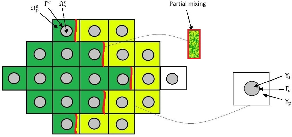
Figure 1. (left) Porous medium $\Omega=\Omega_{p}^{\varepsilon}\cup{\Omega}_{s}^{\varepsilon}$ as a periodic covering of the reference cell $Y=Y_{p}\cup Y_{s}$ (right). The red interface with the partial mixing of the fluids, is the microscopic boundary between two phases occupying the pore space $\Omega_{p}^{\varepsilon}$.

boundary of $\Omega$, respectively; $(c).$ $\Omega$ is periodic, i.e., the solid parts in $\Omega$ are periodically distributed, and is covered by a a finite union of the cells $Y_{k}=Y+k,k\in\mathbb{Z}_{n}$. $Y_{p_{k}}\coloneqq\varepsilon{Y_{p}+k}$, $Y_{s_{k}}\coloneqq\varepsilon{Y_{s}+k}$ and $\Gamma_{s_{k}}=\bar{Y}_{p_{k}}\cap\bar{Y}_{s_{k}}$; $(d).$ for a scale parameter $\varepsilon>0$, we denote the pore space, solid parts and the union of the boundaries of the solid matrices in $\Omega$ by $\Omega_{p}^{\varepsilon}$, $\Omega_{s}^{\varepsilon}$ and $\Gamma^{\varepsilon}$; $(e).$ the boundaries $\Gamma,\Gamma_{s},\Gamma^{\varepsilon},\partial\Omega\in C^{2}$. We denote the volume elements of $\Omega$ and $Y$ by $\,dx$ and $\,dy$, and the surface elements on $\Gamma$ and $\Gamma^{\varepsilon}$ by $\,d\sigma_{x}$ and $\,d\sigma_{y}$, respectively, see figure 1; $(f).$ for $T>0$, $S\coloneqq[0,T)$ be the time interval. The required model under investigation at the micro scale is given by

$$\partial_{t}\mathbf{u}^{\varepsilon}-\mu\varepsilon^{2}\Delta\mathbf{u}^{\varepsilon}+\nabla p^{\varepsilon} =-\varepsilon\lambda c^{\varepsilon}\nabla w^{\varepsilon} S\times\Omega_{p}^{\varepsilon},$$ (1.6a)

$$\nabla.\mathbf{u}^{\varepsilon} =0 S\times\Omega_{p}^{\varepsilon},$$ (1.6b)

$$\mathbf{u}^{\varepsilon} =0 S\times\partial\Omega_{p}^{\varepsilon},$$ (1.6c)

$$\partial_{t}c^{\varepsilon}+\varepsilon\mathbf{u}^{\varepsilon}\cdot\nabla c^{\varepsilon} =\varepsilon^{2}\Delta w^{\varepsilon} S\times\Omega_{p}^{\epsilon},$$ (1.6d)

$$w^{\varepsilon} =-\Delta c^{\varepsilon}+f(c^{\varepsilon}) S\times\Omega_{p}^{\epsilon},$$ (1.6e)

$$\partial_{n}c^{\varepsilon} =\partial_{n}w^{\varepsilon}=0 S\times\partial\Omega_{p}^{\varepsilon},$$ (1.6f)

$$c^{\varepsilon}(0,x) =c_{0}(x) \Omega_{p}^{\varepsilon},$$ (1.6g)

Let $\theta\in[0,1]$ and $1\leq r,s\leq\infty$ be such that $\frac{1}{r}+\frac{1}{s}=1$. Assume that $\Xi\in\{\Omega,\Omega_{p}^{\varepsilon},\Omega_{s}^{\varepsilon}\}$ and $l\in\mathbb{N}_{0}$, then as usual, $L^{r}(\Xi)$ and $H^{l,r}(\Xi)$ denote the Lebesgue and Sobolev spaces with their usual norms and are denoted by $||.||_{r}$ and $||.||_{l,r}$. Similarly, $C^{\theta}(\bar{\Xi})$, $(\cdot,\cdot)_{\theta,r}$ and $[\cdot,\cdot]_{\theta}$ are the Hölder, real- and complex-interpolation spaces respectively endowed with their standard norms, for definition one may refer to [14]. $C^{\alpha}_{\#}(Y)$ denotes the set of all Y-periodic $\alpha$-times continuously differentiable functions in $y$ for $\alpha\in\mathbb{N}$. In particular, $C_{\#}(Y)$ is the space of all the Y-periodic continuous functions in $y$. The $C^{\infty}$-spaces are as usual, equipped with their maximum norm, whereas the space of all continuous functions $C(\Xi)$ is furnished with supremum norm, cf. [14]. The symbol $(.,.)_{H}$ represents the inner product on a Hilbert space H, and $||.||_{H}$ denotes the corresponding norm. For a Banach space $X$, $X^{*}$ denotes its dual and the duality pairing is denoted by $\langle.\;,\;.\rangle_{X^{*}\times X}$. For $p=2,\,H^{1,2}=H^{1}$ and $H^{1}_{0}(\Xi)^{*}=H^{-1}(\Xi)$, where subscript $0$ stands for zero trace. We use the following notations for the function spaces: $\mathcal{U}=\{\mathbf{u}\in\mathcal{D}(\overline{\Omega})^{d}:\divergence\mathbf{u}=0,\mathbf{u}|_{\partial\Omega}=0\},\quad\mathcal{C}=\{c\in\mathcal{D}(\overline{\Omega}):\partial_{n}c=\partial_{n}\Delta c=0\text{ on }\partial\Omega\}.$ We further define $L^{2}_{0}(\Omega^{\epsilon}_{p})=\{\zeta\in L^{2}(\Omega_{\epsilon}^{p}):\int_{\Omega_{\epsilon}^{p}}\zeta dx=0\}$, $\mathcal{U}_{r}(\Omega)\coloneqq\overline{\mathcal{U}}^{\mathbb{H}^{r}(\Omega)}$, $\mathcal{C}_{r}(\Omega)\coloneqq\overline{\mathcal{C}}^{H^{r}(\Omega)}$, $\mathcal{U}(\Omega)=\overline{\mathcal{U}}^{\mathbb{L}^{2}(\Omega)}$, $\mathcal{C}(\Omega)=\overline{\mathcal{C}}^{L^{2}(\Omega)}$, with $\mathbb{L}^{2}(\Omega)=L^{2}(\Omega)^{d}$ and $\mathbb{H}^{r}(\Omega)=H^{r}(\Omega)^{d}$. The spaces $\mathcal{C}_{r}^{\prime}(\Omega_{p}^{\varepsilon})$ and $\mathcal{U}_{r}^{\prime}(\Omega_{p}^{\varepsilon})$ represent the dual of $\mathcal{C}_{r}(\Omega_{p}^{\varepsilon})$ and $\mathcal{U}_{r}(\Omega_{p}^{\varepsilon})$ with respect to their standard norms.
We numerically solve the model at micro and macro-scale in this paper. As we know, at the micro-scale, the model takes into account the heterogeneities and oscillations present in the coefficients and medium; however, it fails to predict the global behaviour of the model. In such cases, we need to choose the size of step-length so small for numerically simulating the model in order to capture the micro-heterogeneities, which leads to complicated analysis and a large portion of execution time and energy consumption by the computer to get the desired results. This paper gives numerical results of how solutions to the Stokes-Cahn-Hilliard equations behave as $\varepsilon\to 0$. The emphasis is on behavior not seen in the original sharp-interface equations and how these behaviors can be suppressed in the limit. The diffuse-interface solutions are desired to converge to the sharp-interface solutions. However, the existence of such model and the homogenization from the micro to macro-scale in authors’ previous work, cf. [1, 15], shows that there does exist such solutions analytically. We now state the assumptions made for the analysis, weak formulation, existence and homogenization results in a nutshell for the reader’s convenience.

1. $F$ is of class $\mathbb{C}^{2}$, and $F\geq 0$ as physically-relevant functions $F$ are always bounded from below, and so the equations remain unchanged by adding a constant to $F$.

2. $\exists~{}\mathcal{K}_{1},\mathcal{K}_{2}>0$ such that $|f(x)|\leq\mathcal{K}_{1}|x|^{p}+\mathcal{K}_{2}$, $|f^{\prime}(x)|\leq\mathcal{K}_{1}|x|^{p-1}+\mathcal{K}_{2}$, $\forall x\in\mathbb{R}$.

3. $\forall\gamma\in\mathbb{R}$, $\exists~{}\mathcal{K}_{3}(\gamma)>0$, $\mathcal{K}_{4}(\gamma)\geq 0$ such that $(x-\gamma)f(x)\geq\mathcal{K}_{3}F(x)-\mathcal{K}_{4}(\gamma)$, $\forall x\in\mathbb{R}$
   where $1\leq p<+\infty$ if $d=2$ and $1\leq p\leq 3$ if $d=3$.

4. $\exists~{}\mathcal{K}_{5}\geq 0$ such that $f^{\prime}\geq-\mathcal{K}_{5}$, $\forall x\in\mathbb{R}$.

5. for all $x\in\Omega$, $\mathbf{u_{0}}$, $c_{0}$ and $w_{0}\geq 0$.

6. $\mathbf{u_{0}}\in L^{\infty}(\Omega)\cap H^{1}(\Omega)$, $c_{0}\in L^{\infty}(\Omega)\cap H^{1}(\Omega)$ and $w^{0}\in L^{\infty}(\Omega)\cap H^{1}(\Omega)$ such that $\sup_{\varepsilon>0}||\mathbf{u_{0}}||_{L^{\infty}(\Omega)\cap H^{1}(\Omega)}<\infty,$ $\sup_{\varepsilon>0}||c_{0}||_{L^{\infty}(\Omega)\cap H^{1}(\Omega)}<\infty,$ $\sup_{\varepsilon>0}||{w_{0}}||_{L^{\infty}(\Omega)\cap H^{1}(\Omega)}<\infty$.

Definition 1.1 (Weak formulation, cf. [15]).

Let the assumptions A1-A6 be satisfied. A quadruple $(c^{\varepsilon},w^{\varepsilon},\mathbf{u}^{\varepsilon},p^{\varepsilon})\in\mathfrak{C}^{\varepsilon}\times\mathfrak{W}^{\varepsilon}\times\mathfrak{V}^{\varepsilon}\times\mathfrak{P}^{\varepsilon}$ is a weak solution of $\mathcal{(P^{\varepsilon})}$ if $c^{\varepsilon},\mathbf{u}^{\varepsilon}$ satisfy $c^{\varepsilon}\in\mathfrak{C}^{\varepsilon}\cap C^{0}\left([0,T);\mathcal{C}_{1}(\Omega_{p}^{\varepsilon})\right)$, $\mathbf{u}^{\varepsilon}\in\mathfrak{V}^{\varepsilon}\cap C^{0}\left([0,T);\mathcal{U}^{\prime}_{\frac{d-2}{4}}(\Omega_{p}^{\varepsilon})\right),$ the initial conditions $(c^{\varepsilon},w^{\varepsilon},\mathbf{u}^{\varepsilon})(0,x)=(c_{0},w_{0},\mathbf{u}_{0})(x)$ for all $x\in\Omega_{p}^{\varepsilon}$, and

$$\left\langle\frac{\mathop{}\!\mathrm{d}c^{\varepsilon}}{\mathop{}\!\mathrm{d}t},\phi\right\rangle+\varepsilon^{2}\int_{\Omega_{p}^{\varepsilon}}\nabla w^{\varepsilon}\cdot\nabla\phi\,dx-\varepsilon\int_{\Omega_{p}^{\varepsilon}}c^{\varepsilon}(\mathbf{u}^{\varepsilon}\cdot\nabla\phi)\,dx=0\quad in\;\mathcal{D}([0,T)),$$ (1.7a)

$$\int_{\Omega_{p}^{\varepsilon}}w^{\varepsilon}\psi\,dx=\int_{\Omega_{p}^{\varepsilon}}\nabla c^{\varepsilon}\cdot\nabla\psi\,dx+\langle f(c^{\varepsilon}),\psi\rangle\qquad in\;\mathcal{D}([0,T)).$$ (1.7b)

$$\left\langle\frac{\mathop{}\!\mathrm{d}\mathbf{u}^{\varepsilon}}{\mathop{}\!\mathrm{d}t},\eta\right\rangle+\mu\varepsilon^{2}\int_{\Omega_{p}^{\varepsilon}}\nabla\mathbf{u}^{\varepsilon}\colon\nabla\eta\,dx=-\varepsilon\lambda\int_{\Omega_{p}^{\varepsilon}}c^{\varepsilon}(\eta\cdot\nabla w^{\varepsilon})\,dx\quad in\;\mathcal{D}([0,T)),$$ (1.7c)

for any $\phi$ in $\mathcal{C}_{1}(\Omega_{p}^{\varepsilon})$, $\psi$ in $\mathcal{C}_{1}(\Omega_{p}^{\varepsilon})$ and $\eta$ in $\mathcal{U}_{1}(\Omega_{p}^{\varepsilon})$. where $\mathcal{U}_{1}(\Omega_{p}^{\varepsilon}),\mathcal{C}_{1}(\Omega_{p}^{\varepsilon})$. We associate a pressure $p^{\varepsilon}\coloneqq\partial_{t}P^{\varepsilon}$ with each weak solution $(c^{\varepsilon},w^{\varepsilon},\mathbf{u}^{\varepsilon})$, which satisfies (1.6a) in the distributional sense, cf. [1].

Theorem 1.1 (Existence, cf. [1, 15]).

Let $d=2$. Assume that $c_{0}\in\mathcal{C}_{1}(\Omega_{p}^{\varepsilon})$, $\mathbf{u}_{0}\in\mathcal{U}(\Omega_{p}^{\varepsilon})$ with $\norm{c_{0}}_{L^{\infty}(\Omega)}\leq 1$ and $\absolutevalue{m(c_{0})}<1$. Also, $F$ satisfies the assumptions A1-A4 stated in section 2.1 of [15], then for any $T>0$, there exists a global weak solution $(\mathbf{u}^{\varepsilon},c^{\varepsilon},w^{\varepsilon})$ to the problem $\mathcal{(P^{\varepsilon})}$ in the sense of definition 3.1 of [15], which satisfies

$$\norm{c^{\varepsilon}-\overline{c^{\varepsilon}}}_{L^{\infty}(S;\mathcal{C}_{1}(\Omega_{p}^{\varepsilon})}+\norm{\mathbf{u}^{\varepsilon}}_{L^{\infty}(S;\mathcal{U}(\Omega_{p}^{\varepsilon}))}+\norm{w^{\varepsilon}}_{L^{2}(S;\mathcal{C}(\Omega_{p}^{\varepsilon}))}+\norm{\partial_{t}c^{\varepsilon}}_{L^{2}(S;\mathcal{C}_{1}^{\prime}(\Omega_{p}^{\varepsilon}))}+\norm{\partial_{t}\mathbf{u}^{\varepsilon}}_{L^{2}(S;\mathcal{U}_{1}^{\prime}(\Omega_{p}^{\varepsilon}))}$$

$$+\frac{\varepsilon}{2}\norm{\nabla w^{\varepsilon}}_{L^{2}(S\times\Omega_{p}^{\varepsilon})^{d}}+\norm{c^{\varepsilon}-\overline{c^{\varepsilon}}}_{L^{2}(S;\mathcal{C}(\Omega_{p}^{\varepsilon}))}+\sqrt{\mu}\varepsilon\norm{\nabla\mathbf{u}^{\varepsilon}}_{L^{2}(S;\mathcal{U}(\Omega_{p}^{\varepsilon})))}+\norm{c^{\varepsilon}-\overline{c^{\varepsilon}}}_{L^{2}(S;\mathcal{C}_{2}(\Omega_{p}^{\varepsilon}))}$$

$$\leq C\left(c_{0},\mathbf{u}_{0},T\right),$$ (1.8)

where the constant $C$ is independent of $\varepsilon$. Furthermore, to prove a result concerning strong solutions to $\mathcal{(P^{\varepsilon})}$, we assume that $F$ is of $C^{3}$-class, and there exists a non-negative $C^{\prime}$ such that

$$\absolutevalue{f^{\prime\prime}(x)}\leq C^{\prime}\left(1+\absolutevalue{x}^{r}\right),~{}\text{ for }r<+\infty,~{}~{}\forall x\in\mathbb{R},$$ (1.9)

Theorem 1.2 (Upscaled Problem $\mathcal{(P)}$, cf. [1, 15]).

Let the assumptions A1 - A6 be satisfied. Then, there exists a limit $(\mathbf{u},c,w)\in\mathfrak{U}\times\mathfrak{C}\times\mathfrak{W}$ of $(c^{\varepsilon},w^{\varepsilon},\mathbf{u^{\varepsilon}})$, such that $(c,w,\mathbf{u})$ satisfies the following problem:

$$\partial_{t}c(x) =\Delta_{y}w(x,y), \Omega_{S}\times Y_{p},$$ (1.10a)

$$\overline{w}(x)+\Delta_{x}c(x)+\nabla_{x}\cdot\overline{\nabla_{y}c_{1}}(x) =f(c(x)), \Omega_{S},$$ (1.10b)

$$\nabla_{y}\cdot\nabla_{y}c_{1}(x,y) =0, \Omega_{S}\times Y_{p}$$ (1.10c)

$$c(0,x) =c_{0}(x), \Omega,$$ (1.10d)

$$\partial_{t}\mathbf{u}(x,y)-\mu\Delta_{y}\mathbf{u}(x,y)+\nabla_{y}p_{1}(x,y)+\nabla_{x}p(x) =-\lambda c(x)\nabla_{y}w(x,y), \Omega_{S}\times Y_{p},$$ (1.10e)

$$\nabla_{y}\cdot\mathbf{u}(x,y) =0, \Omega_{S}\times Y_{p},$$ (1.10f)

$$\nabla_{x}\cdot\overline{\mathbf{u}}(x) =0, \Omega_{S},$$ (1.10g)

$$\bar{\mathbf{u}}(x)\cdot\mathbf{n} =0, \partial\Omega_{S},$$ (1.10h)

$$\mathbf{u}(x,y) =0, \Omega_{S}\times\Gamma_{s},$$ (1.10i)

$$\mathbf{u}(0,x) =\mathbf{u}_{0}(x), \Omega,$$ (1.10j)

where $\Omega_{S}\coloneqq S\times\Omega$, $\partial\Omega_{S}\coloneqq S\times\partial\Omega$ and $\overline{g(x)}\coloneqq\frac{1}{\absolutevalue{Y_{p}}}\int_{Y_{p}}g(x,y)\,dy$ represents the mean of quantity $g$ over the pore part $Y_{p}$ for $x\in\Omega$. Also, $c_{1}(t,x,y)=\phi(t,x)\varsigma(y)$ satisfies (1.10c), where $\varsigma(y)$ is a linear function. We note that $w(x,y)=\partial_{t}c(x)\xi(y)$ from (1.10a), which leads to the following cell problem:

$$\begin{cases}&\partial_{y_{i}y_{j}}\xi(y)=\delta_{ij}\quad\text{ in }Y_{p},\\ &\mathbf{n}\cdot\nabla_{y}\xi(y)=0\quad\text{ on }\partial Y_{p},\\ &\xi(y)\text{ is $Y_{p}$-periodic}.\end{cases}$$

The systems of equations (1.10a)-(1.10j) is the required upscaled model to the system (1.6a)-(1.6g).

2. Simulation of the model

Physical setting of the model. We consider a mixture of two fluids with space variable in $\Omega\subset\mathbb{R}^{2}$, with equal densities and viscosities $\rho_{1}=\rho_{2}=1$ and $\mu_{1}=\mu_{2}=10^{-2}$, and present a computational study to demonstrate the effect of different surface tension parameters. We consider the domain $\Omega=[0,1.2]\times[0,1.0]$ and prescribe homogeneous Dirichlet boundary conditions for the velocity field and homogeneous Neumann boundary conditions for $c$, $w$.

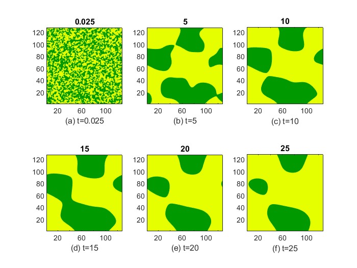
Figure 2. Evolution of the concentration of the two component mixture in 25 seconds (from left to right).

The unit reference cell $Y$ is as usual taken to be $[0,1]\times[0,1]$. The initial condition for the velocity and concentration are assumed to be: $\mathbf{u}_{0}(x_{1},x_{2})=\mathbf{1}$, $c_{0}(x_{1},x_{2})=x_{1}+3$. Further, we set $\lambda=4\times 10^{-2}$, $\varepsilon=5\times 10^{-2}$, $p=0.05$ and begin the simulations for the red interface residing in the pore part of the domain, see figure 1, where the partial mixing of two fluids is captured. We compute until a steady state is reached inside the interfacial region. We choose the free energy potential $F(x)=16~{}b~{}x^{2}(x-1)^{2}$ with $f(x)=F^{\prime}(x)=32~{}b~{}(2x^{3}-3x^{2}+x)$, and chemical potential $w=f(c)-a~{}\Delta c$, where $a$, $b$ are non-negative numbers. We solve the system of equations (1.6) at the micro scale for T = 25 s, i.e. $S=(0,25]$, with the time-step $5\times 10^{-3}$. To be more specific, we perform 5000 simulation in the software MATLAB R2022a version and obtain the following results for the model at micro and macro scale.

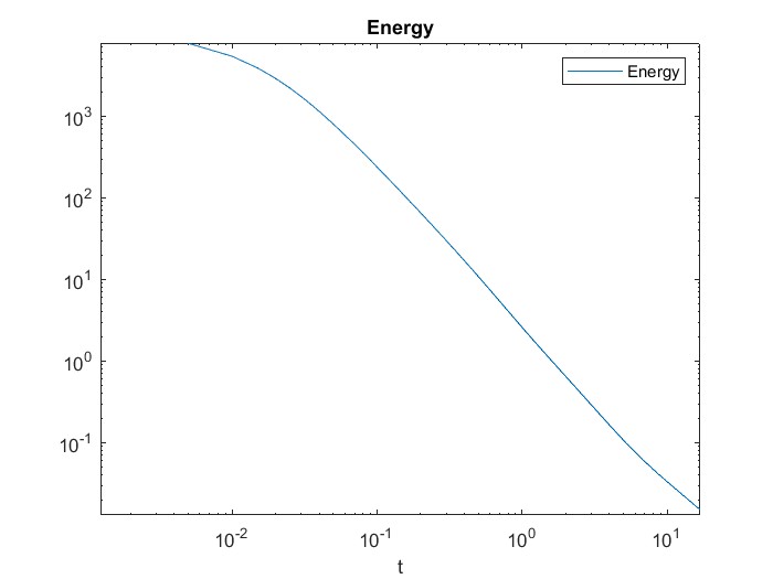
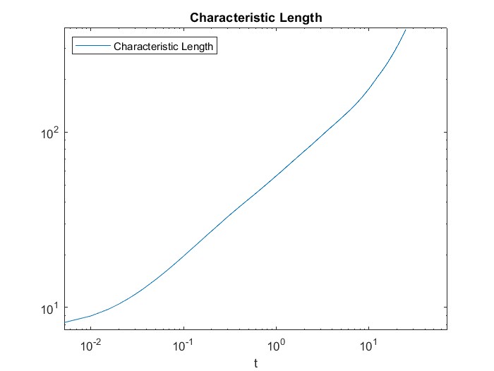
Figure 3. Evolution of the interfacial energy of the two component mixture.

Figure 4. Evolution of the interfacial length of the two component mixture.

2.1. Simulation at the Micro Scale

We choose $a=12$, $b=2$. We set the order parameter $\underline{\mathbf{c}}$ to be a $128\times 128$ matrix and set the variables and initial conditions accordingly, as described earlier, in order to get the contour plots for better visualization of concentration changes with time.

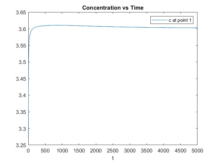
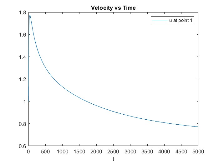
Figure 5. Concentration of one component at a fixed point.

Figure 6. Velocity of one component at a fixed point.

After performing the simulations, for time $t=0.025$ s, $t=5$ s, $t=10$ s, $t=15$ s, $t=20$ s and $t=25$ s, we get the plots, as depicted in the figure 2. We witness the desired phase separation (from left to right). Next, we plot the graph between interfacial energy with time, see figure 4, and interfacial length with time, see figure 4. To see the concentration and velocity variations at different points during the simulations, we choose two reference points $(0.2251,0.1876)$ and $(0.0111,0.0093)$. At the reference point $(0.2251,0.1876)$, we draw graphs for the concentration $c$ and velocity $\mathbf{u}$ in $\Omega_{p}^{\varepsilon}$ in $25$ s, see figure 6, 6. Similarly, at the reference point $(0.0111,0.0093)$, we plot the graphs for concentration $c$ and velocity $\mathbf{u}$ in $\Omega$ in $25$ s, see figure 8, 8.

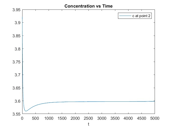
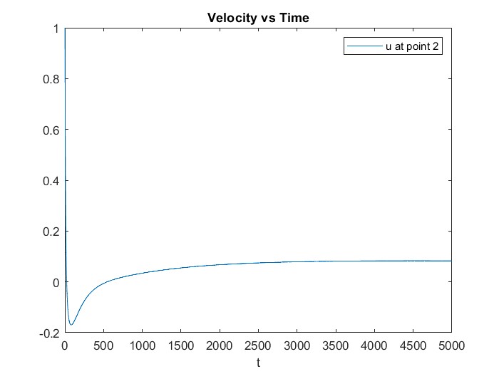
Figure 7. Concentration of one component at a fixed point.

Figure 8. Velocity of one component at a fixed point.

2.2. Simulation at the Macro Scale

We choose $a=10$, $b=1$. We again set $\underline{\mathbf{c}}$ as a $128\times 128$ matrix in order to get the contour plots for better visualization purpose. After performing the simulations, for time $t=0.025$ s, $t=5$ s, $t=10$ s, $t=15$ s, $t=20$ s and $t=25$ s, we get the plots, as depicted in the figure 9.

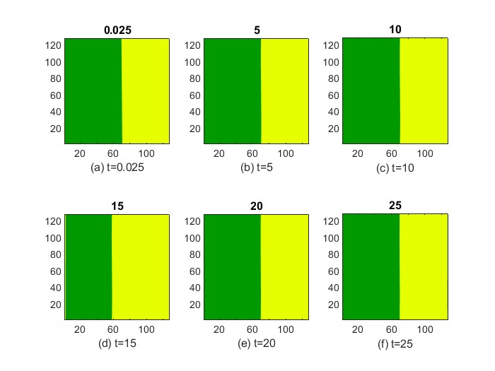
Figure 9. Evolution of the concentration of the two component mixture in 25 seconds (from left to right).

We witness the desired phase separation and the sharp interface over the diffused one. Next, we plot the graph between interfacial energy with time, see figure 11, and interfacial length with time, see figure 11. To see the concentration and velocity variations at different points during the simulations, we choose two reference points $(0.2251,0.1876)$ and $(0.0111,0.0093)$.

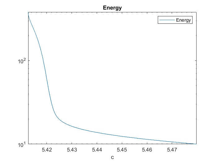
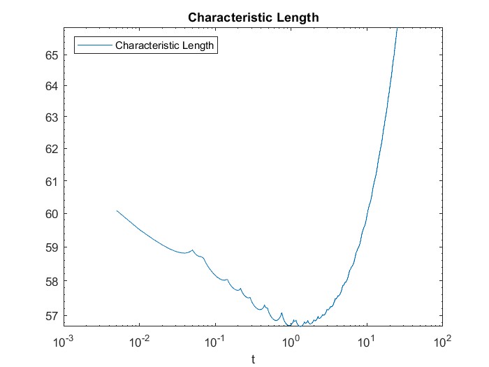
Figure 10. Evolution of the interfacial energy of the two component mixture with concentration.

Figure 11. Evolution of the interfacial length of the two component mixture.

At the reference point $(0.2251,0.1876)$, we draw graphs for the concentration $c$ and velocity $\mathbf{u}$ in $\Omega_{p}^{\varepsilon}$ in $25$ s, see figure 13, 13. Similarly, at the reference point $(0.0111,0.0093)$, we plot the graphs for concentration $c$ and velocity $\mathbf{u}$ in $\Omega$ in $25$ s, see figure 15, 15.

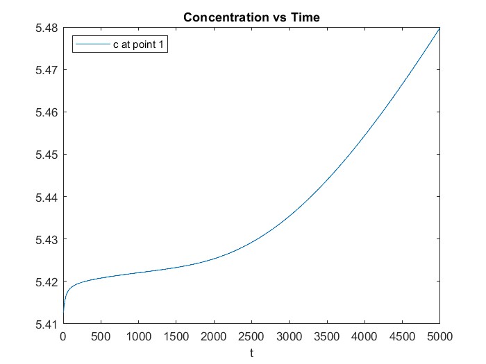
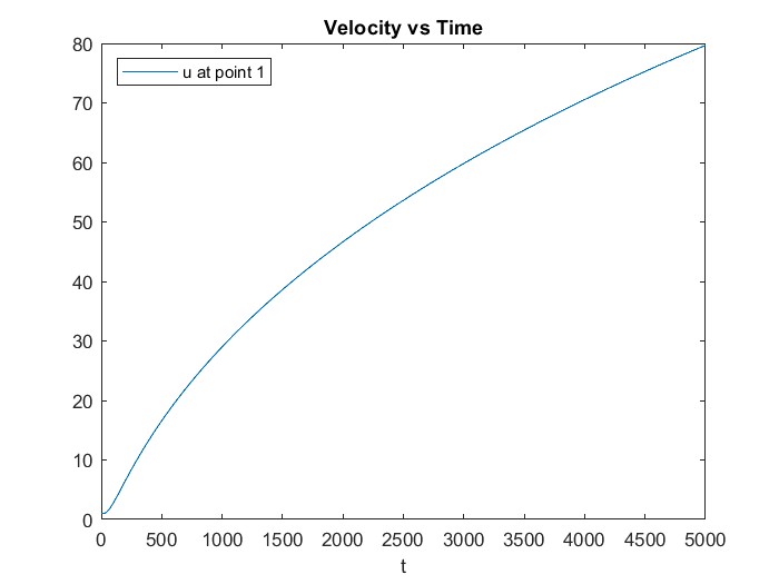
Figure 12. Concentration of one component at a fixed point.

Figure 13. Velocity of one component at a fixed point.

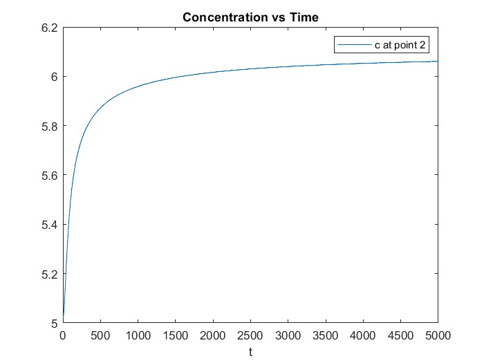
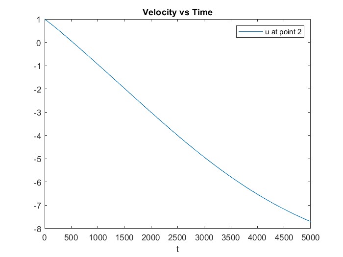
Figure 14. Concentration of one component at a fixed point.

Figure 15. Velocity of one component at a fixed point.

3. Conclusions

We studied a phase-field model for a mixture of two immiscible incompressible components in the context of a porous medium. The model considers surface tension effects and results in a strongly coupled system of Stokes-Cahn-Hilliard equations at the micro-scale. Using the homogenization techniques, we obtain the model at the macro-scale. In this article, we aim to perform numerical experiments on the authors’ previous work, cf. [1, 15]. We observe that the upscaled model has more advantages than the micro one for numerical simulations, as it takes less time than the micro-model, and it will reduce the computational cost while monitoring real-world problems. Furthermore, the numerical simulations for a test problem show that the homogenized equation’s solution approximates the microscopic model’s solution very well. In this way, we validate the homogenization procedure and establish that it is an efficient tool for dealing with such heterogeneous problems.

4. Acknowledgment

The first author would like to thank the Indian Institute of Technology Kharagpur for providing the funding for her PhD position.

5. Conflict of interest

The authors declare no conflict of interest.

References

- [1] N. Lakhmara and H. S. Mahato, “Homogenization of a coupled incompressible stokes–cahn–hilliard system modeling binary fluid mixture in a porous medium,” Nonlinear Analysis, vol. 222, p. 112927, 2022.
- [2] D. Jacqmin, “Calculation of two-phase navier–stokes flows using phase-field modeling,” Journal of computational physics, vol. 155, no. 1, pp. 96–127, 1999.
- [3] M. A. Peter, “Modelling and homogenisation of reaction and interfacial exchange in porous media,” 2003.
- [4] J. Kim, “Phase-field models for multi-component fluid flows,” Communications in Computational Physics, vol. 12, no. 3, pp. 613–661, 2012.
- [5] K. R. Daly and T. Roose, “Homogenization of two fluid flow in porous media,” Proceedings of the Royal Society A: Mathematical, Physical and Engineering Sciences, vol. 471, no. 2176, p. 20140564, 2015.
- [6] L. Baňas and H. S. Mahato, “Homogenization of evolutionary stokes–cahn–hilliard equations for two-phase porous media flow,” Asymptotic Analysis, vol. 105, no. 1-2, pp. 77–95, 2017.
- [7] F. Boyer and C. Lapuerta, “Study of a three component cahn-hilliard flow model,” ESAIM: Mathematical Modelling and Numerical Analysis, vol. 40, no. 4, pp. 653–687, 2006.
- [8] M. Schmuck, M. Pradas, G. A. Pavliotis, and S. Kalliadasis, “Derivation of effective macroscopic stokes–cahn–hilliard equations for periodic immiscible flows in porous media,” Nonlinearity, vol. 26, no. 12, p. 3259, 2013.
- [9] L. Baňas and R. Nürnberg, “Numerical approximation of a non-smooth phase-field model for multicomponent incompressible flow,” ESAIM: Mathematical Modelling and Numerical Analysis, vol. 51, no. 3, pp. 1089–1117, 2017.
- [10] M. I. M. Copetti and C. M. Elliott, “Numerical analysis of the cahn-hilliard equation with a logarithmic free energy,” Numerische Mathematik, vol. 63, no. 1, pp. 39–65, 1992.
- [11] I. Babuvška and W. C. Rheinboldt, “Error estimates for adaptive finite element computations,” SIAM Journal on Numerical Analysis, vol. 15, no. 4, pp. 736–754, 1978.
- [12] J. W. Barrett, R. Nürnberg, and V. Styles, “Finite element approximation of a phase field model for void electromigration,” SIAM Journal on Numerical Analysis, vol. 42, no. 2, pp. 738–772, 2004.
- [13] H. S. Mahato, “Numerical simulations for a two-scale model in a porous medium,” Numerical Analysis and Applications, vol. 10, pp. 28–36, 2017.
- [14] L. Evans, Partial differential equations. AMS Publication, 1998.
- [15] N. Lakhmara and H. S. Mahato, “Homogenization of a diffused interface model with flory-huggins logarithmic potential in a porous medium,” arXiv preprint, July 2022.