Hydrodynamics of a $d$-dimensional long jumps diffusive
symmetric exclusion with a slow barrier

Abstract.

We obtain the hydrodynamic limit of symmetric long-jumps exclusion in $\mathbb{Z}^{d}$ (for $d\geq 1$), where the jump rate is inversely proportional to a power of the jump’s length with exponent $\gamma+1$, where $\gamma\geq 2$. Moreover, movements between $\mathbb{Z}^{d-1}\times\mathbb{Z}_{-}^{*}$ and $\mathbb{Z}^{d-1}\times\mathbb{N}$ are slowed down by a factor $\alpha n^{-\beta}$ (with $\alpha>0$ and $\beta\geq 0$). In the hydrodynamic limit we obtain the heat equation in $\mathbb{R}^{d}$ without boundary conditions or with Neumann boundary conditions, depending on the values of $\beta$ and $\gamma$. The (rather restrictive) condition in [7] (for $d=1$) about the initial distribution satisfying an entropy bound with respect to a Bernoulli product measure with constant parameter is weakened or completely dropped.

1. Introduction

One of the most famous challenges in Thermodynamics is to describe the space/time evolution of a physical quantity of interest in a fluid, such as the density of a gas. However, since the number of molecules is extremely large (of the order of Avogadro’s number), a purely deterministic approach applying Newton’s laws is not feasible. Fortunately, it is possible to go around this issue by using concepts from Statistical Mechanics, where the macroscopic behavior of a fluid is analyzed from the rules governing the microscopic movements of its molecules.

This was the motivation of Spitzer when he introduced the Interacting Particle Systems (IPS) to the mathematical community in [18] as a possible research direction. In many cases, one studies models with a huge number of particles, that move through the sites of a lattice and whose evolution is described by random rules. One remarkable example of an IPS is the exclusion process, where the exclusion rule ensures that every site is occupied by at most one particle. Despite its simplicity it is a model that has been extensively studied in the literature because it captures many interesting phenomena that is shared by many other more complicated dynamics.

In this work, we study the exclusion process evolving on $\mathbb{Z}^{d}$, whose dynamics swaps the position of particles according to some transition probability, therefore the number of particles is the conserved quantity in the system. This motivates the investigation of the space/time evolution of the density of particles, since the total mass is conserved by the dynamics. This description is given by the derivation of a partial differential equation (PDE), known in the literature of IPSs as the hydrodynamic limit.

In this article, we combined the main features of the models presented in [7] and [12]. More specifically, we consider a symmetric exclusion process where particles move on a $d-$dimensional lattice and there exists a slow barrier hindering some of the (possibly long) jumps. This is quite an interesting feature, since multidimensional IPSs are much less common in the literature than the unidimensional ones. More precisely, particles move according to a probability transition $p:\mathbb{Z}^{d}\rightarrow[0,1]$, given by

$$p(\hat{x})=\begin{dcases}\frac{c_{\gamma}|\hat{x}|^{-\gamma-1}}{d},&\quad\text{if}\;\;\hat{x}\neq\hat{0}\;\;\text{and}\;\;\exists j\in\{1,\ldots,d\}:\hat{x}=\pm|\hat{x}|\hat{e}_{j};\\ 0,&\quad\text{otherwise}.\end{dcases}$$ (1.1)

Above, $\gamma\geq 2$ (the inclusion of the case $\gamma=2$ is an improvement on the conditions imposed upon the model in [7], where it was assumed $\gamma>2$), $c_{\gamma}$ is a normalizing constant and $\{\hat{e}_{1},\ldots,\hat{e}_{d}\}$ is the canonical basis of $\mathbb{R}^{d}$. From (1.1), we see that diagonal jumps are forbidden. For instance, when $d=2$ it is not possible for a particle to move from $(1,3)$ directly to $(4,8)$ with only one jump; it must move first to an intermediate site, such as $(4,3)$ or $(1,8)$. The reason for this choice of $p(\cdot)$ is due to the fact that in this work we want to obtain the heat equation, written in terms of the Laplacian operator in dimension $d$, which is given by $\Delta=\sum_{j=1}^{d}\partial_{\hat{e}_{j}}\partial_{\hat{e}_{j}}$. Indeed, for every $j$ fixed, the effect of only considering jumps in the direction determined by $\hat{e}_{j}$ leads to $\partial_{t}\rho=\partial_{\hat{e}_{j}}\partial_{\hat{e}_{j}}\rho$ (analogously to the results in [7]), see (3.6) and Lemma B.1 for more details.

Next, we add a barrier hindering the jumps between $\mathbb{Z}^{d-1}\times\mathbb{Z}_{-}^{*}$ and $\mathbb{Z}^{d-1}\times\mathbb{N}$, where $\mathbb{N}:=\{0,1,\ldots\}$ and $\mathbb{Z}_{-}^{*}:=\mathbb{Z}-\mathbb{N}=\{-1,-2,\ldots\}$. In the same way as it is done in [7] and [12], the slowing factor is $\alpha n^{-\beta}$, with $n\geq 1$, $\alpha>0$ and $\beta\geq 0$. We stress that only (some of the) movements affecting the last coordinate are affected. For instance, for $d=2$, the jump rate from $(-2,-2)$ to $(-2,2)$ is multiplied by $\alpha n^{-\beta}$; on the other hand jumps from $(-2,-3)$ to $(-2,-4)$, from $(-1,-3)$ to $(2,-3)$ and from $(2,1)$ to $(2,-1)$ are not realized through slow bonds. This is illustrated in Figure 1 below. The slow barrier hinders the transport of mass between $\mathbb{R}^{d-1}\times(-\infty,0)$ and $\mathbb{R}^{d-1}\times[0,\infty)$, leading to Neumann boundary conditions when $\beta$ is large enough.

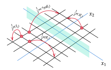
Figure 1. Dynamics of the long-jumps symmetric exclusion with slow bonds in $\mathbb{Z}^{2}$. The factor $1/2$ comes from $d=2$. Recall from (1.1) that $p(2\hat{e}_{1})=p(-2\hat{e}_{1})$ and $p(\hat{e}_{2})=p(-\hat{e}_{2})$.

We observe that this work is a non-trivial generalization of the results in [7, 12]. Indeed, in [7, 12], the initial distribution needs to satisfy an entropy bound with respect to a reference measure, the Bernoulli product measure of constant parameter (this is analogous to the case where $h$ in Definition 2.4 is taken as being constant). This assumption simplified the proofs and in [7], it was fundamental to derive global energy estimates, since the spatial domain was unbounded.

In previous works (see [7, 8]), those global energy estimates could not be dispensed, since they were crucial to prove the uniqueness of weak solutions according to Oleinik’s procedure; this uniqueness is, in turn, essential to obtain the hydrodynamic limit by using the tools of the entropy method introduced in [14]. In this work, by dropping the assumption that $h$ in Definition 2.4 is constant, we can treat a much larger class of initial profiles in our system, therefore Theorem 2.11 is much more general than the main result in [7] for most of the values for $(\beta,\gamma)$. Furthermore, for a slightly smaller range of values of $(\beta,\gamma)$, we can avoid any kind of entropy bounds, see Theorem 2.10.

Here, the setting is also substantially different from [12], since our spatial domain is unbounded, in opposition to the later one. A bounded spatial domain (such as the one in [12, 17] is particularly simpler in a multidimensional context, since it allows us to define the density at the boundary in the sense given by the Trace Theorem (Theorem 1 in Section 5.5 of [9]). However, we do not have this possibility in this work and we only present some definition of the density at the boundary for the particular case when $d=1$. This can be done since local energy estimates ensure that the density has a continuous representative in the neighborhood of the origin, see Proposition 2.5 for more details.

The only drawback of this work, in comparison with [7], is to treat the very particular case where $d=1$, $\gamma>2$ and $\beta=1$. In order to apply the entropy method in this case, we would have to prove the uniqueness of weak solutions with a space of test functions satisfying Robin boundary conditions, and unfortunately we were not able to obtain this particular result. So far, we were only able to treat this case by assuming an entropy bound with respect to the product measure given by Definition 2.4 when $h$ is constant. Since this assumption is exactly the same as in [7], we did not treat this case here.

Next we describe the outline of this article. In Section 2 we give the details of our model, we define the notions of weak solutions that are deduced and we state the hydrodynamic limit. In Section 3 we motivate the definitions of weak solutions presented in the previous section. In Section 4 we present the tightness of the sequence of empirical measures. In Section 5 we characterize the limiting point by showing that it is concentrated on a Dirac measure of a trajectory of measures which are absolutely continuous with respect to the Lebesgue measure, whose density is a weak solution of the corresponding hydrodynamic equation. Section 6 is devoted to the proof of some estimates which are applied in the proofs of the results of the previous section. Finally in Section 7 we treat the case $d=1$ and $\gamma>2$ in order to be able to define the density at the origin. Sections 6 and 7 both make use of Proposition 6.4, whose proof is postponed to Appendix C.

We complement the article with three appendices: Appendix A is devoted to the proof of uniqueness of weak solutions for our hydrodynamic equations, Appendix B is focused on the convergence from the discrete operators to the continuous ones, Appendix C presents a variety of bounds which were useful to show Proposition 6.4 and Appendix D is dedicated to the proof of the tightness criterium that we use since the process is evolving in infinite volume.

2. Statement of results

2.1. The model

For every $k\geq 1$ and $u_{1},\ldots u_{k}\in\mathbb{R}$, we will denote the maximum norm of a vector $(u_{1},\ldots,u_{k})\in\mathbb{R}^{k}$ by

$$|(u_{1},\ldots,u_{k})|:=\max\{|u_{1}|,\ldots,|u_{k}|\}.$$

Hereinafter, we fix a dimension $d\in\mathbb{Z}^{*}_{+}=\{1,2,3,\ldots,\}$ and we represent elements of $\mathbb{R}^{d}$ with a hat, e.g., $\hat{u}=(u_{1},\ldots,u_{d})$, unless we assume that $d=1$. We also make use of the canonical basis $\{\hat{e}_{1},\ldots,\hat{e}_{d}\}$ of $\mathbb{R}^{d}$. Usually we denote elements of $\mathbb{R}^{d}$ by $\hat{u}$ and $\hat{v}$.

Our goal is to study the space-time evolution of the density of particles in the symmetric exclusion process with long jumps evolving on the lattice $\mathbb{Z}^{d}$. This is a stochastic interacting particle system which allows at most one particle per site, therefore our space state is $\Omega:=\{0,1\}^{\mathbb{Z}^{d}}$. The elements of the lattice $\mathbb{Z}^{d}$ are called sites and will be denoted by Latin letters, such as $\hat{x}$, $\hat{y}$ and $\hat{z}$. The elements of $\Omega$ are called configurations and will be denoted by Greek letters, such as $\eta$. Moreover, we denote the number of particles at a site $\hat{x}$ on a configuration $\eta$ by $\eta(\hat{x})$; this means that the site $\hat{x}$ is empty (resp. occupied) if $\eta(\hat{x})=0$ (resp. $\eta(\hat{x})=1$).

The transition probability is denoted by $p:\mathbb{Z}^{d}\rightarrow[0,1]$ and it is given by (1.1). Since we want to observe a diffusive behavior, $\gamma\in[2,\infty)$ and $c_{\gamma}$ is a constant that turns $p(\cdot)$ into a probability. For $d=1$ and $\gamma>2$, we recover the long-jumps form of the probability distribution given in [7]. This motivates us to the denote (for the case $\gamma>2$) $\sigma^{2}:=d\sum_{r}r^{2}p(r\hat{e}_{d})=2d\sum_{r=1}^{\infty}c_{\gamma}r^{1-\gamma}<\infty$.

We observe that our dynamics does not allow diagonal jumps: therefore, after a direction determined by $\hat{e}_{j}$ is chosen, a particle can only jump from $\hat{x}=(x_{1},\ldots,x_{j-1},x_{j},x_{j+1},\ldots,x_{d})$ to $\hat{y}=(x_{1},\ldots,x_{j-1},y_{j},x_{j+1},\ldots,x_{d})$, for some $y_{j}\neq x_{j}$. This motivates us to write $\hat{u}=(\hat{u}_{\star,j},u_{j})$, where $\hat{u}_{\star,j}$ is the element of $\mathbb{R}^{d-1}$ constructed by removing the $j$-th coordinate of $\hat{u}$. In the particular case $j=d$, we use the notation $\hat{u}_{\star}:=\hat{u}_{\star,d}$.

According to the exclusion rule, given two sites $\hat{x},\hat{y}$, a particle only goes from $\hat{x}$ to $\hat{y}$ if the later one is empty and the former one is occupied, i.e. $\eta(\hat{y})=0$ and $\eta(\hat{x})=1$. This means that a movement between $\hat{x}$ and $\hat{y}$ only is possible if $\eta(\hat{x})[1-\eta(\hat{y})]+\eta(\hat{y})[1-\eta(\hat{x})]=1$. This operation acts on an initial configuration $\eta\in\Omega$ and transforms it into $\eta^{\hat{x},\hat{y}}\in\Omega$, that is defined by

$$\eta^{\hat{x},\hat{y}}(\hat{z})=\begin{cases}\eta(\hat{y}),&\quad\hat{z}=\hat{x};\\ \eta(\hat{x}),&\quad\hat{z}=\hat{y};\\ \eta(\hat{z}),&\quad\hat{z}\notin\{\hat{x},\hat{y}\}.\end{cases}$$

The elements of ${\mathcalboondox B}:=\big{\{}\{\hat{x},\hat{y}\}:\hat{x}\neq\hat{y}\in\mathbb{Z}^{d}\big{\}}$ are called bonds. We denote $\mathbb{N}:=\{0,1,2,\ldots\}$ $\mathbb{Z}_{-}^{*}:=\mathbb{Z}-\mathbb{N}=\{-1,-2,\ldots\}$, and ${\mathcalboondox S}:=\big{\{}\{\hat{x},\hat{y}\}\in{\mathcalboondox B}:\hat{x}\in\mathbb{Z}^{d-1}\times\mathbb{Z}_{-}^{*},\,\hat{y}\in\mathbb{Z}^{d-1}\times\mathbb{N}\big{\}}$. Moreover, we denote ${\mathcalboondox F}:={\mathcalboondox B}-{\mathcalboondox S}$.

Next we introduce a slow barrier in the system. Here we fix $\alpha>0$ and $\beta\geq 0$. Starting from a configuration $\eta$, a particle jumps from $\hat{x}$ to $\hat{y}$ at rate $\eta(\hat{x})[1-\eta(\hat{y})]r_{\hat{x},\hat{y}}^{n}$, where

$$r_{\hat{x},\hat{y}}^{n}:=\begin{cases}\alpha n^{-\beta},&\quad\{\hat{x},\hat{y}\}\in{\mathcalboondox S};\\ 1,&\quad\{\hat{x},\hat{y}\}\in{\mathcalboondox F}.\end{cases}$$ (2.1)

When $\beta>0$, we have $\lim_{n\rightarrow\infty}r_{\hat{x},\hat{y}}^{n}=0$ for every $\{\hat{x},\hat{y}\}$ in ${\mathcalboondox S}$, creating a physical barrier between $\mathbb{Z}^{d-1}\times\mathbb{Z}_{-}^{*}$ and $\mathbb{Z}^{d-1}\times\mathbb{N}$. Then ${\mathcalboondox S}$ and ${\mathcalboondox F}$ are the sets of slow and fast bonds, respectively.

We say that a function $f:\Omega\rightarrow\mathbb{R}$ is local if there exists a finite set $\Lambda\subset\mathbb{Z}^{d}$ such that

$$\forall\hat{x}\in\Lambda,\quad\eta_{1}(\hat{x})=\eta_{2}(\hat{x})\Rightarrow f(\eta_{1})=f(\eta_{2}).$$

Finally, the exclusion process with slow bonds is defined by the infinitesimal generator ${\mathcalboondox L}_{n}$, given by

$$({\mathcalboondox L}_{n}f)(\eta):=\sum_{\hat{x},\hat{y}}p(\hat{y}-\hat{x})\eta(\hat{x})[1-\eta(\hat{y})]r_{\hat{x},\hat{y}}^{n}\nabla_{\hat{x},\hat{y}}f(\eta)=\frac{1}{2}\sum_{\hat{x},\hat{y}}p(\hat{y}-\hat{x})r_{\hat{x},\hat{y}}^{n}\nabla_{\hat{x},\hat{y}}f(\eta),$$

where $\nabla_{\hat{x},\hat{y}}f(\eta):=[f(\eta^{\hat{x},\hat{y}})-f(\eta)]$ $f$ is a local function. In last line and in what follows, unless it is stated differently, we will assume that our discrete variables in a summation always range over $\mathbb{Z}^{d}$.

2.2. Notation

In this subsection, we begin by presenting the notation for some spaces of test functions. For every $r\in\mathbb{N}$, we denote by $C_{c}^{r}(\mathbb{R}^{d})$ the space of functions which are in $C^{r}(\mathbb{R}^{d})$ and have a compact support; this means that there exists $b_{1}>0$ such that $G(\hat{u})=0$ for $|\hat{u}|\geq b_{1}$. We also denote the space of functions $G:[0,\infty)\times\mathbb{R}^{d}\rightarrow\mathbb{R}$ with compact support $K\subset[0,\infty)\times\mathbb{R}$ which are of class $r_{1}$ regarding the temporal variable and of class $r_{2}$ regarding the spatial variable by $C_{c}^{r_{1},r_{2}}([0,\infty)\times\mathbb{R}^{d})$.

For every $j\in\{1,\ldots,d\}$, we denote by $\partial_{\hat{e}_{j}}G$ the partial derivative of $G$ in the direction of $\hat{e}_{j}$, i.e.

$$\partial_{\hat{e}_{j}}G(\hat{u}):=\lim_{h\rightarrow 0}\frac{G(\hat{u}+h\hat{e}_{j})-G(\hat{u})}{h}$$

when the above limit exists. We are aware of the more usual notation $\partial_{x_{j}}G$, but we will not use the later notation in order to avoid confusion with $x_{j}$, the $j$-th coordinate of the site $\hat{x}\in\mathbb{Z}^{d}$. Similarly, we denote the second derivative of $G$ in the direction determined by $\hat{e}_{j}$ by $\partial_{\hat{e}_{j}\hat{e}_{j}}G$. We do not make use of the notations $\partial_{x_{j}}G$ and $\partial_{x_{j}x_{j}}G$ in order to avoid confusion with $x_{j}$, the $j$-th coordinate of the site $\hat{x}\in\mathbb{Z}^{d}$. Naturally, the Laplacian of $G$ is $\Delta G:=\sum_{j=1}^{d}\partial_{\hat{e}_{j}\hat{e}_{j}}G$. In the particular case $d=1$, we denote $\partial_{\hat{e}_{d}}$ by $\nabla$. Finally, if $G:\mathbb{R}\rightarrow\mathbb{R}$ is bounded, we denote $\|G\|_{\infty}:=\sup_{u\in\mathbb{R}}|G(u)|$.

When $\beta\in[0,1)$, the slow bonds are not strong enough to have a macroscopic effect in our system, and this motivates the choice of ${\mathcalboondox S}_{Dif}:=C_{c}^{1,2}([0,\infty)\times\mathbb{R}^{d})$ as the space of test functions. On the other hand, when $\beta\geq 1$, the slow bonds will hinder the flow of mass between $\mathbb{R}_{-}^{d*}:=\mathbb{R}^{d-1}\times(-\infty,0)$ and $\mathbb{R}_{+}^{d*}:=\mathbb{R}^{d-1}\times[0,\infty)$, leading to functions which may be discontinuous at $\mathcal{H}:=\{\hat{u}\in\mathbb{R}^{d}:u_{d}=0\}$. This motivates the following definition:

$${\mathcalboondox S}_{Disc}:=\{G:[0,\infty)\times\mathbb{R}^{d}\rightarrow\mathbb{R}:\exists G^{-},G^{+}\in{\mathcalboondox S}_{Dif}\;\;\text{s.t.}\;\;G=\mathbbm{1}_{\{[0,\infty)\times\mathbb{R}_{-}^{d*}\}}G^{-}+\mathbbm{1}_{\{[0,\infty)\times\mathbb{R}_{-}^{d*}\}}G^{+}\}.$$

In particular, by choosing $G^{-}=G^{+}$, we get ${\mathcalboondox S}_{Dif}\subsetneq{\mathcalboondox S}_{Disc}$.

In order to observe a macroscopic influence of the slow bonds in our system, our Markov process will be accelerated in time by a factor of $\Theta(n)$, given by

$$\Theta(n):=\begin{cases}n^{2},&\quad\gamma>2;\\ n^{2}/\log(n),&\quad\gamma=2.\end{cases}$$ (2.2)

We make this choice in order to obtain a convergence (as $n\rightarrow\infty$) of a discrete operator to the Laplacian operator in $L^{1}(\mathbb{R}^{d})$, see Proposition 3.1 for more details. We study the process $\eta_{t}^{n}(\cdot):=\eta_{t\Theta(n)}(\cdot)$, whose infinitesimal generator is given by $\Theta(n){\mathcalboondox L}_{n}$. We fix $T>0$, which leads to a finite time horizon $[0,T]$. We always assume that we start from a configuration in $\Omega$, therefore the exclusion rule ensures that $(\eta^{n}_{t})_{t\in[0,T]}\in{\mathcalboondox D}([0,T],\Omega)$, the space of (right-continuous and with left limits) trajectories in $\Omega$.

Given a measure space $(X,\mu)$, for every $p\in[1,\infty]$ let $L^{p}(X):=L^{p}(X,\mu)$. In this work, $\mu$ is the Lebesgue measure on $X$. We also denote the norm in $L^{p}(X)$ by $\|\cdot\|_{p,X}$ for $p<\infty$ and by $\|\cdot\|_{\infty}$ for $p=\infty$. Moreover, given $f,g\in L^{2}(\mathbb{R}^{d})$, we define

$$\langle f,g\rangle:=\int_{\mathbb{R}^{d}}f(\hat{u})g(\hat{u})\,d\hat{u}.$$

Definition 2.1.

We denote the space of non-negative Radon measures on $\mathbb{R}^{d}$ endowed with the vague topology by ${\mathcalboondox M}^{+}$.

The empirical measure, denoted by $\pi^{n}$, is defined by

$$\pi^{n}(\eta,\,d\hat{u}):=\frac{1}{n^{d}}\sum_{\hat{x}}\eta(\hat{x})\delta_{\frac{\hat{x}}{n}}(d\hat{u}),$$ (2.3)

where $\delta_{\hat{v}}$ is the Dirac measure on $\hat{v}\in\mathbb{R}^{d}$. Denoting $\pi_{t}^{n}:=\pi^{n}(\eta_{t}^{n},\,d\hat{u})$, we produce a Markov process $(\pi^{n}_{t})_{t\in[0,T]}\in{\mathcalboondox D}([0,T],{\mathcalboondox M}^{+})$, the space of the càdlàg (right-continuous and with left limits) trajectories on ${\mathcalboondox M}^{+}$. We use the following notation for the integral of a function $G$ with respect to $\pi_{t}^{n}$:

$$\forall G\in L^{1}(\mathbb{R}^{d}),\forall t\in[0,T],\quad\langle\pi_{t}^{n},G\rangle:=\frac{1}{n^{d}}\sum_{\hat{x}}\eta_{t}^{n}(\hat{x})G(\tfrac{\hat{x}}{n}).$$ (2.4)

Definition 2.2.

We say that the sequence $(\mu_{n})_{n\geq 1}$ of probability measures on $\Omega$ is associated to a measurable profile $g:\mathbb{R}^{d}\rightarrow[0,1]$ if

$$\lim_{n\rightarrow\infty}\mu_{n}\big{(}\eta\in\Omega:|\langle\pi^{n},G\rangle-\langle g,G\rangle|>\delta\big{)}=0,$$ (2.5)

for every $\delta>0$ and every $G\in C_{c}^{0}(\mathbb{R}^{d})$. This means that the sequence of random empirical measures $\pi^{n}(\eta,d\hat{u})$ converges weakly to the deterministic measure $g(\hat{u})d\hat{u}$ in ${\mathcalboondox M}^{+}$, which can be interpreted as a weak Law of Large Numbers.

We denote by $(\mathbb{P}_{\mu_{n}})_{n\geq 1}$ (resp. $(\mathbb{Q}_{n})_{n\geq 1}$) the sequence of probability measures on ${\mathcalboondox D}([0,T],\Omega)$ (resp. ${\mathcalboondox D}([0,T],{\mathcalboondox M}^{+})$) induced by a given sequence $(\mu_{n})_{n\geq 1}$ of probability measures on $\Omega$. We also denote the expectation with respect to $\mathbb{P}_{\mu_{n}}$ by $\mathbb{E}_{\mu_{n}}$.

In this work we fix a measurable profile $g:\mathbb{R}^{d}\rightarrow[0,1]$ and a sequence $(\mu_{n})_{n\geq 1}$ of probability measures on $\Omega$ associated to $g$. This means that (2.5) holds for $t=0$ and want to prove that $\pi^{n}(\eta_{t}^{n},d\hat{u})$ converges weakly to a deterministic measure $\rho(t,\hat{u})d\hat{u}$, in some sense, for every $t\in[0,T]$. We will also prove that $\rho:[0,T]\times\mathbb{R}^{d}\rightarrow[0,1]$ is a weak solution of a partial differential equation (PDE), the hydrodynamic equation. In this work, the PDE will be the heat equation, since we want to observe a diffusive behavior, and for this reason we made the choice $\gamma\geq 2$.

2.2.1. Product measures

Next we introduce a class of product measures defined on the state space $\Omega$ which will be relevant later on.

Definition 2.3.

We say that $h:\mathbb{R}^{d}\rightarrow[0,1]$ is a reference profile if it satisfies the following conditions:

1. $h$ is bounded away from the boundary of $[0,1]$, i.e., there exist $a_{h}<b_{h}$ in $(0,1)$ such that $h(\hat{u})\in[a_{h},b_{h}]$, for every $\hat{u}\in\mathbb{R}^{d}$;

2. $h$ is Lipschitz, i.e., there exists $L_{h}>0$ such that $|h(\hat{v})-h(\hat{u})|\leq L_{h}|\hat{v}-\hat{u}|$, for every $\hat{u},\hat{v}\in\mathbb{R}^{d}$;

3. $h$ is constant far from the origin, i.e., there exist $A_{h}\in[a_{h},b_{h}]$ and $K_{h}>0$ such that $h(\hat{u})=A_{h}$ when $|\hat{u}|\geq K_{h}$.

We denote the space of reference profiles by $Ref$. An element of $Ref$ is analogous to the profile $h$ introduced in [4, 5]. Moreover (in the same way as it was done in [4, 5]), for every $h\in Ref$ and $n\geq 1$ we define a probability measure $\nu_{h}^{n}$ on $\Omega$.

Definition 2.4.

Let $h\in Ref$ and $n\geq 1$. We denote by $\nu_{h}^{n}$ the Bernoulli product measure on $\Omega$ with marginals given by

$$\forall\hat{x}\in\mathbb{Z}^{d},\;\;1-\nu_{h}^{n}\big{(}\eta(\hat{x})=0\big{)}=\nu_{h}^{n}\big{(}\eta(\hat{x})=1\big{)}=h(\tfrac{\hat{x}}{n}).$$

In order to use a procedure analogous to the one in [11, 10, 4, 13, 5, 3], in many cases we will require the following assumption:

$$\exists h\in Ref:H(\mu_{n}|\nu_{h}^{n})\lesssim n^{d}.$$ (2.6)

Above the notation $f(n)\lesssim g(n)$ means that there exists $C>0$ satisfying $0\leq f(n)\leq Cg(n)$, $n\geq 1$.

2.2.2. Sobolev spaces

In this subsubsection, we assume $d=1$. Moreover, in this work we always assume that $I\subset\mathbb{R}$ is an open interval and $\bar{I}$ is the closure of $I$. Next we introduce the notation for Sobolev spaces, following Chapter 8 of [6]. We say that $G\in{\mathcalboondox H}^{1}(I)$ if $G\in L^{2}(I)$ and there exists $g\in L^{2}(I)$ such that

$$\forall\phi\in C_{c}^{\infty}(I),\;\int_{\mathbb{R}}G(u)\partial_{1}\phi(u)\,du=-\int_{\mathbb{R}}g(u)\phi(u)\,du.$$

We denote $g$ by $\partial_{u}G$, and it is the weak derivative of $G$. We remark that ${\mathcalboondox H}^{1}(I)$ is a Hilbert space with norm given by $\|G\|^{2}_{{\mathcalboondox H}^{1}(I)}:=\|G\|^{2}_{2,I}+\|\partial_{u}G\|^{2}_{2,I}$. Next we present a classical result stated in [6], whose proof comes from a direct application of Hölder’s inequality.

Proposition 2.5.

For any $f\in{\mathcalboondox H}^{1}(I)$, there exists $\tilde{f}:\bar{I}\rightarrow\mathbb{R}$ such that $f=\tilde{f}$ almost everywhere on $I$ and $|\tilde{f}(v_{2})-\tilde{f}(v_{1})|\leq\|f\|_{{\mathcalboondox H}^{1}(I)}|v_{2}-v_{1}|^{1/2}$, for every$v_{1},v_{2}\in\bar{I}$.

We say $f\in{\mathcalboondox H}_{loc}^{1}(\mathbb{R}^{*})$ if there exist $a_{1},a_{2}>0$ and two intervals $I_{1}=(-a_{1},0)$ and $I_{2}=(0,a_{2})$ such that $f|_{I_{j}}\in{\mathcalboondox H}^{1}(I_{j})$, $j=1,2$. From Proposition 2.5, every $f\in{\mathcalboondox H}^{1}(I)$ has an unique continuous representative $\tilde{f}$ defined on $\bar{I}$, the closure of $I$, in the sense that $\tilde{f}(u)=f(u)$, almost everywhere in $I$. In particular, if $f\in{\mathcalboondox H}_{loc}^{1}(\mathbb{R}^{*})$, then $f$ has unique continuous representatives in $[-a_{1},0]$ and $[0,a_{2}]$, and the limits

$$f(0^{-}):=\lim_{\varepsilon\rightarrow 0^{+}}\int_{-\varepsilon}^{0}f(u)\,du;\quad f(0^{+}):=\lim_{\varepsilon\rightarrow 0^{+}}\int_{0}^{\varepsilon}f(u)\,du;$$

are well-defined. In next subsection, we describe the hydrodynamic equations that can we obtain; they depend on whether we are assuming (2.6) or not, and on the values of $\alpha$, $\beta$ and $\gamma$.

2.3. Hydrodynamic equations

We begin with the hydrodynamic equation obtained when $(\alpha,\beta)=(1,0)$ (i.e., $\alpha=1$ and $\beta=0$). Hereinafter, for every time-dependent function $f$ we denote its temporal derivative by $\partial_{t}f$. Moreover, for every $s\in[0,T]$, we denote $f_{s}:=f(s,\cdot):\mathbb{R}^{d}\rightarrow\mathbb{R}$.

Definition 2.6.

Let $\kappa>0$ and $g:\mathbb{R}^{d}\rightarrow[0,1]$ be a measurable function. Then $\rho:[0,T]\times\mathbb{R}^{d}\rightarrow[0,1]$ is a weak solution of the heat equation with initial condition $g$

$$\begin{cases}\partial_{t}\rho_{t}(\hat{u})=\kappa\Delta\rho_{t}(\hat{u}),&\quad(t,\hat{u})\in[0,T]\times\mathbb{R}^{d},\\ \rho_{0}(\hat{u})=g(\hat{u}),&\quad\hat{u}\in\mathbb{R}^{d},\end{cases}$$ (2.7)

if for every $t\in[0,T]$ and for every $G\in{\mathcalboondox S}_{\textrm{Dif}}$, we have $F_{\textrm{Dif}}(t,\rho,G,g,\kappa)=0$, where

$$F_{\textrm{Dif}}(t,\rho,G,g,\kappa):= \int_{\mathbb{R}^{d}}\rho_{t}(\hat{u})G_{t}(\hat{u})\,d\hat{u}-\int_{\mathbb{R}^{d}}g(\hat{u})G_{0}(\hat{u})\,d\hat{u}-\int_{0}^{t}\int_{\mathbb{R}^{d}}\rho_{s}(\hat{u})[\kappa\Delta+\partial_{s}]G_{s}(\hat{u})\,d\hat{u}\,ds.$$

Next we present the heat equation with Neumann boundary conditions; we observe that the elements of the space of test functions satisfy Neumann boundary conditions themselves. Observe that $\partial_{\hat{e}_{d}}$ is the partial derivative in the direction determined by $\hat{e}_{d}$, which is normal to the hyperplan $\mathcal{H}$.

Definition 2.7.

Let $\kappa>0$ and $g:\mathbb{R}^{d}\rightarrow[0,1]$ be a measurable function. Then $\rho:[0,T]\times\mathbb{R}^{d}\rightarrow[0,1]$ is a weak solution of the heat equation with Neumann boundary conditions and initial condition $g$

$$\begin{cases}\partial_{t}\rho_{t}(\hat{u})=\kappa\Delta\rho_{t}(\hat{u}),&\quad(t,\hat{u})\in[0,T]\times\mathbb{R}^{d},\\ \partial_{\hat{e}_{d}}\rho_{t}(\hat{u}_{\star},0^{+})=\partial_{\hat{e}_{d}}\rho_{t}(\hat{u}_{\star},0^{-})=0,&\quad t\in(0,T],\;\hat{u}_{\star}\in\mathcal{H},\\ \rho_{0}(\hat{u})=g(\hat{u}),&\quad\hat{u}\in\mathbb{R}^{d},\end{cases}$$ (2.8)

if for every $G\in{\mathcalboondox S}_{\textrm{Neu}}:=\{G\in{\mathcalboondox S}_{Disc}:\forall s\in[0,T],\forall\hat{u}_{\star}\in\mathcal{H},\quad\partial_{\hat{e}_{d}}G^{-}_{s}(\hat{u}_{\star},0)=\partial_{\hat{e}_{d}}G^{+}_{s}(\hat{u}_{\star},0)=0\}$ and every $t\in[0,T]$, we have $F_{\textrm{Dif}}(t,\rho,G,g,\kappa)=0$.

When (2.6) holds, some technical results (known in the literature as Replacement Lemmas) can be derived. Under that assumption, for $d=1$ and $\gamma>2$ we can treat a wider space of test functions, such as ${\mathcalboondox S}_{Disc}$ instead of ${\mathcalboondox S}_{Neu}$. This wider space leads to a new integral equation, given by $F_{\textrm{Neu}}$ below.

Definition 2.8.

Let $\kappa>0$ and $g:\mathbb{R}\rightarrow[0,1]$ be a measurable function. Then $\rho:[0,T]\times\mathbb{R}\rightarrow[0,1]$ is a weak solution of the heat equation with Neumann boundary conditions and initial condition $g$

$$\begin{cases}\partial_{t}\rho_{t}(u)=\kappa\Delta\rho_{t}(u),&\quad(t,u)\in[0,T]\times\mathbb{R}^{*},\\ \nabla\rho_{t}(0^{+})=\nabla\rho_{t}(0^{-})=0,&\quad t\in(0,T],\\ \rho_{0}(u)=g(u),&\quad u\in\mathbb{R},\end{cases}$$ (2.9)

if the following two conditions hold:

1. for every $G\in{\mathcalboondox S}_{\textrm{Disc}}$ and every $t\in[0,T]$, we have $F_{\textrm{Neu}}(t,\rho,G,g,\kappa)=0$, where

   $$F_{\textrm{Neu}}(t,\rho,G,g,\kappa):= \int_{\mathbb{R}}\rho_{t}(u)G_{t}(u)\,du-\int_{\mathbb{R}}g(u)G_{0}(u)\,du-\int_{0}^{t}\int_{\mathbb{R}}\rho_{s}(u)[\kappa\Delta+\partial_{s}]G_{s}(u)\,du\,ds$$

   $$+ \kappa\int_{0}^{t}[\nabla G_{s}(0^{-})\rho_{s}(0^{-})-\nabla G_{s}(0^{+})\rho_{s}(0^{+})]\,ds;$$

2. $\rho_{s}\in{\mathcalboondox H}_{loc}^{1}(\mathbb{R}^{*})$, for a.e. $s\in[0,T]$.

Due to $(2)$ in last definition, $\rho_{s}(0^{-})$ and $\rho_{s}(0^{+})$ are well-defined for a.e. $s\in[0,T]$. Combining this with some Replacement Lemmas (which require (2.6)), we are allowed to deal with ${\mathcalboondox S}_{Disc}$ as a space of test functions, which is significantly larger than ${\mathcalboondox S}_{Neu}$, the space of test functions of (2.8). Since all weak solutions of (2.9) are also weak solutions of (2.8), the uniqueness of weak solutions of (2.9) is a direct consequence of the uniqueness of weak solutions of (2.8).

The following result is proved in Appendix A.

Lemma 2.9.

There exists at most one weak solution of (2.7), (2.8) and (2.9).

Now we state the main results of this work. We do not present the results for the case $\beta=1$ and $\gamma>2$, because this case was already treated in Theorem 2.8 of [7].

2.4. Main results

We present two theorems, depending on whether we assume (2.6) or not. We recall that $c_{2}$ is the normalizing constant $c_{\gamma}$ in (1.1) for $\gamma=2$. The following notation will be useful to state the main results in a clean way. Let

$$R_{0}:=\big{(}[1,\infty)\times\{2\}\big{)}\cup\big{(}(1,\infty)\times(2,\infty)\big{)};\quad\kappa_{\gamma}:=\begin{cases}c_{2}/d,&\quad\gamma=2;\\ \sigma^{2}/2d,&\quad\gamma>2.\end{cases}$$ (2.10)

Theorem 2.10.

(Hydrodynamic Limit without an entropy bound) Let $g:\mathbb{R}^{d}\rightarrow[0,1]$ be a measurable function and $(\mu_{n})_{n\geq 1}$ be a sequence of probability measures on $\Omega$ associated to the initial profile $g$. Then, for every $t\in[0,T]$, every $G\in C_{c}^{0}(\mathbb{R}^{d})$ and every $\delta>0$,

$$\lim_{n\rightarrow\infty}\mathbb{P}_{\mu_{n}}\Big{(}\eta^{n}_{\cdot}\in{\mathcalboondox D}([0,T],\Omega):\Big{|}\langle\pi^{n}_{t},G\rangle-\int_{\mathbb{R}^{d}}G(\hat{u})\rho_{t}(\hat{u})\,d\hat{u}\Big{|}>\delta\Big{)}=0,$$

where $\rho$ is the unique weak solution of

$$\begin{cases}\eqref{ehd},\quad\text{with}\quad\kappa=\kappa_{\gamma},&\quad\text{if}\quad(\alpha,\beta)=(1,0)\quad\text{and}\quad\gamma\geq 2;\\ \eqref{ehdn},\quad\text{with}\quad\kappa=\kappa_{\gamma},&\quad\text{if}\quad\alpha>0\quad\text{and}\quad(\beta,\gamma)\in R_{0}.\end{cases}$$

When we assume (2.6), we are able to obtain a result for a wider range of values of $(\alpha,\beta,\gamma)$.

Theorem 2.11.

(Hydrodynamic Limit with an entropy bound) Let $g:\mathbb{R}^{d}\rightarrow[0,1]$ be a measurable function and $(\mu_{n})_{n\geq 1}$ be a sequence of probability measures on $\Omega$ associated to the initial profile $g$ satisfying (2.6). Then, for every $t\in[0,T]$, every $G\in C_{c}^{0}(\mathbb{R}^{d})$ and every $\delta>0$,

$$\lim_{n\rightarrow\infty}\mathbb{P}_{\mu_{n}}\Big{(}\eta^{n}_{\cdot}\in{\mathcalboondox D}([0,T],\Omega):\Big{|}\langle\pi^{n}_{t},G\rangle-\int_{\mathbb{R}^{d}}G(\hat{u})\rho_{t}(\hat{u})\,d\hat{u}\Big{|}>\delta\Big{)}=0,$$

where $\rho$ is the unique weak solution of

$$\begin{cases}\eqref{ehd},\quad\text{with}\quad\kappa=\kappa_{\gamma},&\quad\text{if}\quad(\alpha,\beta,\gamma)\in(0,\infty)\times[0,1)\times[2,\infty)\quad\text{and}\quad d\geq 1;\\ \eqref{ehdn},\quad\text{with}\quad\kappa=\kappa_{\gamma},&\quad\text{if}\quad\alpha>0\quad\text{and}\quad(\beta,\gamma)\in R_{0}\quad\text{and}\quad d\geq 2;\\ \eqref{ehdnlee},\quad\text{with}\quad\kappa=\kappa_{\gamma},&\quad\text{if}\quad(\alpha,\beta,\gamma)\in(0,\infty)\times(1,\infty)\times(2,\infty)\quad\text{and}\quad d=1.\end{cases}$$

The rest of this work is devoted to the proof of the two previous theorems. In Section 4, we prove that the sequence $(\mathbb{Q}_{n})_{n\geq 1}$ is tight with respect to the Skorohod topology of ${\mathcalboondox D}([0,T],{\mathcalboondox M}^{+})$ and therefore it has at least one limiting point $\mathbb{Q}$. We prove that any limit point $\mathbb{Q}$ is concentrated on trajectories that satisfy the first (resp. second) condition of weak solutions of the corresponding hydrodynamic equations from the results of Sections 5 and 6 (resp. Section 7). The necessary Replacement Lemmas are proved in Section 6 and the uniqueness of weak solutions to the hydrodynamic equations is derived in Appendix A. Finally, we present some auxiliary results in Appendices B, C and D. We stress that the uniqueness of weak solutions to the corresponding hydrodynamic equation implies the uniqueness of the limit point $\mathbb{Q}$ and the convergence of the sequence $(\mathbb{Q}_{n})_{n\geq 1}$, leading to the desired result.

3. Heuristic argument to deduce the hydrodynamic equations

Observe that ${\mathcalboondox S}_{Dif}\subsetneq{\mathcalboondox S}_{Neu}\subsetneq{\mathcalboondox S}_{Disc}$, therefore all test functions in Theorems 2.10 and 2.11 belong to $S_{Disc}$. From Dynkin’s formula, see, for example Appendix 1.5 of [16], for every $t\in[0,T]$ we have that

$${\mathcalboondox M}_{t}^{n}(G)=\langle\pi_{t}^{n},G_{t}\rangle-\langle\pi_{0}^{n},G_{0}\rangle-\int_{0}^{t}\partial_{s}\langle\pi_{s}^{n},G_{s}\rangle\,ds-\int_{0}^{t}\Theta(n){\mathcalboondox L}_{n}\langle\pi_{s}^{n},G_{s}\rangle\,ds,$$ (3.1)

is a martingale for every $G\in{\mathcalboondox S}_{Disc}$ with respect to the natural filtration ${\mathcalboondox F}_{t}^{n}=\sigma(\eta_{s}^{n}:0\leq s\leq t)$. The last term on the right-hand side of (3.1) is known in the literature as the integral term and it will determine which hydrodynamic equation we will obtain, depending on the values of $\alpha$, $\beta$, $\gamma$ and $d$. Next, we perform some (heuristic) computations in order to study the $L^{1}(\mathbb{P}_{\mu_{n}})$-convergence of that integral term. According to this, we define some operators which act on $G\in{\mathcalboondox S}_{Disc}$.

For ${\mathcalboondox C}\in\{{\mathcalboondox B},{\mathcalboondox S}\}$, we define the operator ${\mathcalboondox K}_{n,{\mathcalboondox C}}$ by

$${\mathcalboondox K}_{n,{\mathcalboondox C}}G_{s}(\tfrac{\hat{x}}{n}):=\sum_{\hat{y}:\,\{\hat{x},\hat{y}\}\in{\mathcalboondox C}}[G_{s}(\tfrac{\hat{y}}{n})-G_{s}(\tfrac{\hat{x}}{n})]p(\hat{y}-\hat{x}).$$ (3.2)

Next we treat two different cases: $\beta\in[0,1)$ and $(\beta,\gamma)\in R_{0}$.

I.: Case $\beta\in[0,1)$. In this case the space of test functions is ${\mathcalboondox S}_{Dif}$ and we make use of the next two results. Proposition 3.1 (resp. Proposition 3.2) is proved in Appendix B (resp. Section 6).

Proposition 3.1.

For every $G\in{\mathcalboondox S}_{\textrm{Dif}}$ we have

$$\lim_{n\rightarrow\infty}\frac{1}{n^{d}}\sum_{\hat{x}}\;\sup_{s\in[0,T]}|\Theta(n){\mathcalboondox K}_{n,{\mathcalboondox B}}G_{s}(\tfrac{\hat{x}}{n})-\kappa_{\gamma}\Delta G_{s}(\tfrac{\hat{x}}{n})|=0.$$

Proposition 3.2.

Assume (2.6), $\beta\in[0,1)$ and $t\in[0,T]$. For every $G\in{\mathcalboondox S}_{Dif}$ we have

$$\lim_{n\rightarrow\infty}\mathbb{E}_{\mu_{n}}\Big{[}\Big{|}\int_{0}^{t}\sum_{\hat{x}}\frac{\Theta(n)}{n^{d}}{\mathcalboondox K}_{n,{\mathcalboondox S}}G_{s}\left(\tfrac{\hat{x}}{n}\right)\eta_{s}^{n}(\hat{x})\,ds\Big{|}\Big{]}=0.$$

From the symmetry of $p(\cdot)$, the integral term $\int_{0}^{t}\Theta(n){\mathcalboondox L}_{n}\langle\pi_{s}^{n},G_{s}\rangle ds$ can be rewritten as

$$\int_{0}^{t}\sum_{\hat{x}}\frac{\Theta(n)}{n^{d}}{\mathcalboondox K}_{n,{\mathcalboondox B}}G_{s}\left(\tfrac{\hat{x}}{n}\right)\eta_{s}^{n}(\hat{x})\,ds+\Big{(}1-\frac{\alpha}{n^{\beta}}\Big{)}\int_{0}^{t}\sum_{\hat{x}}\frac{\Theta(n)}{n^{d}}{\mathcalboondox K}_{n,{\mathcalboondox S}}G_{s}\left(\tfrac{\hat{x}}{n}\right)\eta_{s}^{n}(\hat{x})\,ds.$$ (3.3)

Since our Markov process is the exclusion process, it holds

$$\forall n\geq 1,\forall s\in[0,T],\forall\hat{x}\in\mathbb{Z}^{d},\quad 0\leq\eta_{s}^{n}(\hat{x})\leq 1.$$ (3.4)

Therefore, by applying Proposition 3.1 the first term of (3.3) converges, as $n\rightarrow\infty$, to

$$\kappa_{\gamma}\int_{0}^{t}\int_{\mathbb{R}^{d}}\rho_{s}(\hat{u})\Delta G_{s}(\hat{u})\,d\hat{u}\,ds,$$

in $L^{1}(\mathbb{P}_{\mu_{n}})$. Moreover, if $\alpha=1$ and $\beta=0$, the second term of (3.3) is equal to zero. Otherwise, assuming (2.6) this term converges, as $n\rightarrow\infty$, to zero in $L^{1}(\mathbb{P}_{\mu_{n}})$, due to Proposition 3.2. Therefore for $\beta\in[0,1)$ we get in the limit (as $n\rightarrow\infty$) the integral equation in (2.7).

II.: Case $(\beta,\gamma)\in R_{0}$. In this case the space of test functions is ${\mathcalboondox S}_{\gamma,d}$, given by

$${\mathcalboondox S}_{\gamma,d}:=\begin{cases}{\mathcalboondox S}_{Neu},\quad\text{if}\quad\gamma=2\quad\text{or}\quad d\geq 2;\\ {\mathcalboondox S}_{Disc},\quad\text{if}\quad\gamma>2\quad\text{and}\quad d=1.\end{cases}$$ (3.5)

Since the test functions can be discontinuous at $\mathcal{H}$, the operator $\Theta(n){\mathcalboondox K}_{n,{\mathcalboondox B}}G_{s}$ is not assured to converge to $\kappa_{\gamma}\Delta G_{s}$ as $n\rightarrow\infty$ in $L^{1}(\mathbb{Z}^{d})$, as it was the case in Proposition 3.1. In order to address this issue, some adjustments are required. From (1.1), once that the direction of a jump (determined by $\hat{e}_{j}$, for some $j\in\{1,\ldots,d\}$) is chosen, a particle can only move from $(\hat{x}_{\star,j},x_{j})$ to some $(\hat{x}_{\star,j},y_{j})$, for $y_{j}\neq x_{j}$. Therefore ${\mathcalboondox K}_{n,{\mathcalboondox B}}$ can be rewritten as $\sum_{j=1}^{d}{\mathcalboondox K}_{n,j}$, where ${\mathcalboondox K}_{n,j}$ is given by

$${\mathcalboondox K}_{n,j}G_{s}(\tfrac{\hat{x}}{n})={\mathcalboondox K}_{n,j}G_{s}(\tfrac{\hat{x}_{\star,j}}{n},\tfrac{x_{j}}{n}):=\sum_{y_{j}\in\mathbb{Z}}[G_{s}(\tfrac{\hat{x}_{\star,j}}{n},\tfrac{y_{j}}{n})-G_{s}(\tfrac{\hat{x}_{\star,j}}{n},\tfrac{x_{j}}{n})]p\big{(}(y_{j}-x_{j})\hat{e}_{j}\big{)}.$$ (3.6)

From Lemma B.1, $\Theta(n){\mathcalboondox K}_{n,j}G_{s}$ converges to $\kappa_{\gamma}\partial_{\hat{e}_{j}\hat{e}_{j}}G_{s}$ in $L^{1}(\mathbb{Z}^{d})$, as $n\rightarrow\infty$, when $G$ is of class $C^{2}$ along the direction determined by $\hat{e}_{j}$; in particular, Proposition 3.1 is a direct consequence of Lemma B.1. However, for $G\in{\mathcalboondox S}_{Disc}$, $G$ may be discontinuous along the direction determined by $\hat{e}_{d}$, hence we cannot make use of ${\mathcalboondox K}_{n,d}$. Alternatively, we define the operators ${\mathcalboondox R}_{n,d}$ and $\tilde{{\mathcalboondox K}}_{n,d}$ by

$${\mathcalboondox R}_{n,d}G_{s}\left(\tfrac{\hat{x}}{n}\right)={\mathcalboondox R}_{n,d}G_{s}\left(\tfrac{\hat{x}_{\star}}{n},\tfrac{x_{d}}{n}\right):=\begin{dcases}\frac{1}{n}\partial_{\hat{e}_{d}}G_{s}^{+}(\tfrac{\hat{x}_{\star}}{n},0)\sum_{y_{d}=0}^{\infty}(y_{d}-x_{d})p\big{(}(y_{d}-x_{d})\hat{e}_{d}\big{)},&x_{d}\geq 0;\\ \frac{1}{n}\partial_{\hat{e}_{d}}G_{s}^{-}(\tfrac{\hat{x}_{\star}}{n},0)\sum_{y_{d}=-\infty}^{-1}(y_{d}-x_{d})p\big{(}(y_{d}-x_{d})\hat{e}_{d}\big{)},&x_{d}\leq-1.\end{dcases}$$ (3.7)

and

$$\tilde{{\mathcalboondox K}}_{n,d}G_{s}\left(\tfrac{\hat{x}_{\star}}{n},\tfrac{x_{d}}{n}\right):=\begin{dcases}-{\mathcalboondox R}_{n,d}G_{s}\left(\tfrac{\hat{x}_{\star}}{n},\tfrac{x_{d}}{n}\right)+\sum_{y_{d}=0}^{\infty}A^{n,\hat{x}_{\star}}_{x_{d},y_{d}}(G_{s}^{+}),&x_{d}\geq 0;\\ -{\mathcalboondox R}_{n,d}G_{s}\left(\tfrac{\hat{x}_{\star}}{n},\tfrac{x_{d}}{n}\right)+\sum_{y_{d}=-\infty}^{-1}A^{n,\hat{x}_{\star}}_{x_{d},y_{d}}(G_{s}^{-}),&x_{d}\leq-1.\end{dcases}$$ (3.8)

Above, for any $H:\mathbb{R}\rightarrow\mathbb{R}$, any $\hat{x}_{\star}\in\mathbb{Z}^{d-1}$, any $x,y\in\mathbb{Z}$ and $n\geq 1$, $A^{n,\hat{x}_{\star}}_{x_{d},y_{d}}(H)$ is given by

$$A^{n,\hat{x}_{\star}}_{x_{d},y_{d}}(H):=[H(\tfrac{\hat{x}_{\star}}{n},\tfrac{y_{d}}{n})-H(\tfrac{\hat{x}_{\star}}{n},\tfrac{x_{d}}{n})]p\big{(}(y_{d}-x_{d})\hat{e}_{d}\big{)}.$$ (3.9)

From Lemma B.2, $\Theta(n)\tilde{{\mathcalboondox K}}_{n,d}G_{s}$ converges to $\kappa_{\gamma}\partial_{\hat{e}_{d}\hat{e}_{d}}G_{s}$ in $L^{1}(\mathbb{Z}^{d})$, as $n\rightarrow\infty$, when $\gamma=2$ and $G\in{\mathcalboondox S}_{Neu}$ or $\gamma>2$ and $G\in{\mathcalboondox S}_{Disc}$. This motivates us to rewrite the integral term $\int_{0}^{t}\Theta(n){\mathcalboondox L}_{n}\langle\pi_{s}^{n},G_{s}\rangle\,ds$ as

$$\int_{0}^{t}\sum_{\hat{x}}\frac{\Theta(n)}{n^{d}}{\mathcalboondox K}_{n}^{*}G_{s}\left(\tfrac{\hat{x}}{n}\right)\eta_{s}^{n}(\hat{x})\,ds+\alpha\int_{0}^{t}\sum_{x}\frac{\Theta(n)}{n^{d+\beta}}{\mathcalboondox K}_{n,{\mathcalboondox S}}G_{s}(\tfrac{\hat{x}}{n})\eta_{s}^{n}(\hat{x})\,ds$$ (3.10)

$$+ \int_{0}^{t}\sum_{\hat{x}}\frac{\Theta(n)}{n^{d}}{\mathcalboondox R}_{n}G_{s}\left(\tfrac{\hat{x}}{n}\right)\eta_{s}^{n}(\hat{x})\,ds,$$ (3.11)

where ${\mathcalboondox K}_{n}^{*}:=\tilde{{\mathcalboondox K}}_{n,d}+\sum_{j=1}^{d-1}{\mathcalboondox K}_{n,j}$. Thus, we treat the first term of (3.10) with Proposition 3.3 below. This proposition is a direct consequence of Lemmas B.1 and B.2, proved in Appendix B.

Proposition 3.3.

Assume $\gamma=2$ and $G\in{\mathcalboondox S}_{Neu}$ or $\gamma>2$ and $G\in{\mathcalboondox S}_{Disc}$. Then

$$\lim_{n\rightarrow\infty}\frac{1}{n^{d}}\sum_{\hat{x}}\sup_{s\in[0,T]}|\Theta(n){\mathcalboondox K}_{n}^{*}G_{s}(\tfrac{\hat{x}}{n})-\kappa_{\gamma}\Delta G_{s}(\tfrac{\hat{x}}{n})|=0.$$

Applying last result, the first term of (3.10) converges, as $n\rightarrow\infty$, to

$$\kappa_{\gamma}\int_{0}^{t}\int_{\mathbb{R}^{d}}\rho_{s}(\hat{u})\Delta G_{s}(\hat{u})\,d\hat{u}\,ds,$$

in $L^{1}(\mathbb{P}_{\mu_{n}})$. In order to treat the second term of (3.10), it is enough to prove that it holds

$$\forall G\in{\mathcalboondox S}_{Disc},\;\forall(\beta,\gamma)\in R_{0},\quad\lim_{n\rightarrow\infty}\sum_{\hat{x}_{\star}\in\mathcal{H}}\;\sum_{x_{d}\in\mathbb{Z}}\;\sup_{s\in[0,T]}\Big{|}\frac{\Theta(n)}{n^{d+\beta}}{\mathcalboondox K}_{n,{\mathcalboondox S}}G_{s}(\tfrac{\hat{x}_{\star}}{n},\tfrac{x_{d}}{n})\Big{|}=0.$$ (3.12)

From (1.1) and the definition of ${\mathcalboondox S}$, for every $G\in{\mathcalboondox S}_{Disc}$ a particle can only jump between $\hat{x}$ and $\hat{y}$ for $\{\hat{x},\hat{y}\}\in{\mathcalboondox S}$ when there exist $x_{d}\geq 0,y_{d}<0$ or $x_{d}<0,y_{d}\geq 0$ and $\hat{x}_{\star}\in\mathbb{Z}^{d-1}$ such that $\hat{x}=(\hat{x}_{\star},x_{d})$ and $\hat{y}=(\hat{y}_{\star},y_{d})=(\hat{x}_{\star},y_{d})$ (i.e., $\hat{x}_{\star}=\hat{y}_{\star}$). Performing simple algebraic manipulations, we get

$${\mathcalboondox K}_{n,{\mathcalboondox S}}G_{s}(\tfrac{\hat{x}_{\star}}{n},\tfrac{x_{d}}{n}):=\begin{dcases}\sum_{y_{d}=-\infty}^{-1}A^{n,\hat{x}_{\star}}_{x_{d},y_{d}}(G_{s}),\quad&x_{d}\geq 0;\\ \sum_{y_{d}=0}^{\infty}A^{n,\hat{x}_{\star}}_{x_{d},y_{d}}(G_{s}),\quad&x_{d}<0.\end{dcases}$$ (3.13)

Since $G$ has compact support uniformly in time, this leads to

$$\sum_{\hat{x}_{\star}\in\mathbb{Z}^{d-1}}\;\sum_{x_{d}\in\mathbb{Z}}{\mathcalboondox K}_{n,{\mathcalboondox S}}G_{s}(\tfrac{\hat{x}_{\star}}{n},\tfrac{x_{d}}{n})=\sum_{|\hat{x}_{\star}|<b_{G}n}\Big{\{}\sum_{x_{d}=0}^{\infty}\;\sum_{y_{d}=-\infty}^{-1}A^{n,\hat{x}_{\star}}_{x_{d},y_{d}}(G_{s})+\sum_{x_{d}=-\infty}^{-1}\;\sum_{y_{d}=0}^{\infty}A^{n,\hat{x}_{\star}}_{x_{d},y_{d}}(G_{s})\Big{\}},$$ (3.14)

where $b_{G}$ is given by

$$b_{G}:=\inf\{b_{1}>0:|\hat{u}|\geq b_{1}\Rightarrow\sup_{s\in[0,T]}|G_{s}(\hat{u})|=0\}.$$ (3.15)

Indeed, for $|\hat{x}_{\star}|\geq b_{G}n$, we have $G_{s}(\tfrac{\hat{x}_{\star}}{n},\tfrac{y_{d}}{n})=G_{s}(\tfrac{\hat{x}_{\star}}{n},\tfrac{x_{d}}{n})=A^{n,\hat{x}_{\star}}_{x_{d},y_{d}}(G_{s})=0$, for every $x_{d},y_{d}\in\mathbb{Z}$. Thus, from (3.14) and the triangle inequality, the display inside the limit in (3.12) is bounded from above by

$$\frac{\Theta(n)2\|G\|_{\infty}c_{\gamma}}{dn^{d+\beta}}\sum_{|\hat{x}_{\star}|<b_{G}n}\Big{\{}\sum_{x_{d}=0}^{\infty}\;\sum_{y_{d}=-\infty}^{-1}|y_{d}-x_{d}|^{-1-\gamma}+\sum_{x_{d}=-\infty}^{-1}\;\sum_{y_{d}=0}^{\infty}|y_{d}-x_{d}|^{-1-\gamma}\Big{\}}$$

$$\leq\frac{\Theta(n)4\|G\|_{\infty}(2b_{G}n)^{d-1}c_{\gamma}}{dn^{d+\beta}}\sum_{x_{d}=0}^{\infty}\;\sum_{y_{d}=-\infty}^{-1}(x_{d}-y_{d})^{-1-\gamma}\lesssim\frac{\Theta(n)}{n^{1+\beta}}\sum_{z_{d}=1}^{\infty}(z_{d})^{-\gamma}\lesssim\frac{\Theta(n)}{n^{1+\beta}},$$

that goes to zero as $n\rightarrow\infty$, due to (2.2) and the fact that $(\beta,\gamma)\in R_{0}$. Above we used the fact that the sum over $z_{d}$ is convergent, since $\gamma\geq 2>1$. Therefore we have proved (3.12). By combining (3.4) and (3.12), the second term of (3.10) converges, as $n\rightarrow\infty$, to zero in $L^{1}(\mathbb{P}_{\mu_{n}})$. It remains to treat the term in (3.11). When $\gamma=2$ or $d\geq 2$, $G\in{\mathcalboondox S}_{Neu}$, and from (3.7) we get $\partial_{\hat{e}_{d}}G^{+}_{s}(\tfrac{\hat{x}_{\star}}{n},0)=\partial_{\hat{e}_{d}}G^{+}_{s}(\tfrac{\hat{x}_{\star}}{n},0)={\mathcalboondox R}_{n}G_{s}\left(\tfrac{\hat{x}}{n}\right)=0$ for every $\hat{x}\in\mathbb{Z}^{d-1}$ and every $s\in[0,T]$. Therefore, we get the integral equation in (2.8). It remains to analyse $\gamma>2$, $d=1$ and $G\in{\mathcalboondox S}_{Disc}$. Next for $\ell\geq 1$, we define the empirical averages on a box of size $\ell$ around $0$ as

$$\overrightarrow{\eta}^{\ell}(0):=\frac{1}{\ell}\sum_{y_{d}=1}^{\ell}\eta(y_{d})\;\;\text{and}\;\;\overleftarrow{\eta}^{\ell}(0):=\frac{1}{\ell}\sum_{y_{d}=-\ell}^{-1}\eta(y_{d}).$$ (3.16)

Thus, the term in (3.11) can be treated with next result, which is proved in Section 6.

Proposition 3.4.

Assume (2.6), $\gamma>2$, $t\in[0,T]$ and $d=1$. For every $G\in{\mathcalboondox S}_{Disc}$ we have

$$\limsup_{\varepsilon\rightarrow 0^{+}}\limsup_{n\rightarrow\infty}\mathbb{E}_{\mu_{n}}\Big{[}\Big{|}\int_{0}^{t}\Big{\{}\frac{\Theta(n)}{n^{d}}\sum_{x_{d}=0}^{\infty}{\mathcalboondox R}_{n}G_{s}(\tfrac{x_{d}}{n})\eta_{s}^{n}(x_{d})-\kappa_{\gamma}\nabla G_{s}^{+}(0)\overrightarrow{\eta}^{\varepsilon n}_{s}(0)\Big{\}}\,ds\Big{|}\Big{]}=0,$$

$$\limsup_{\varepsilon\rightarrow 0^{+}}\limsup_{n\rightarrow\infty}\mathbb{E}_{\mu_{n}}\Big{[}\Big{|}\int_{0}^{t}\Big{\{}\frac{\Theta(n)}{n^{d}}\sum_{x_{d}=-\infty}^{-1}{\mathcalboondox R}_{n}G_{s}(\tfrac{x_{d}}{n})\eta_{s}^{n}(x_{d})+\kappa_{\gamma}\nabla G_{s}^{-}(0)\overleftarrow{\eta}^{\varepsilon n}_{s}(0)\Big{\}}\,ds\Big{|}\Big{]}=0.$$

From last result, (3.11) converges, as $n\rightarrow\infty$, to

$$\kappa_{\gamma}\int_{0}^{t}[\nabla G_{s}(0^{+})\rho_{s}(0^{+})-\nabla G_{s}(0^{-})\rho_{s}(0^{-})]\,ds$$

in $L^{1}(\mathbb{P}_{\mu_{n}})$, and we get the integral equation in (2.9).

4. Tightness

This section is devoted to the proof of tightness of the sequence $(\mathbb{Q}_{n})_{n\geq 1}$. We will make use of the following definition, which is motivated by the time horizon $[0,T]$.

Definition 4.1.

We denote by $\mathcal{T}_{T}$ the set of stopping times bounded by $T$. Thus, if $t\geq 0$ and $\tau\in\mathcal{T}_{T}$, $\tau+t\mathcal{T}_{T}$ iff $\tau+t:=\min\{\tau+t,T\}$.

In many articles dealing with exclusion processes evolving in a bounded spatial domain, to prove tightness it is enough to invoke Propositions 1.6 and 1.7 in Chapter 4 of [16], see for example [11, 10, 4, 13, 5, 3]. We observe that the later proposition is explicitly stated for processes evolving in bounded spatial domains, therefore rigorously it cannot be directly applied for processes evolving in infinite volume, such as it is our context. To clarify the fact that we can actually use the same results as in the setting of bounded domains, we prove in Appendix D the following technical lemma.

Lemma 4.2.

Assume that for every $\varepsilon>0$,

$$\lim_{\lambda\rightarrow 0^{+}}\varlimsup_{n\rightarrow\infty}\sup_{\tau\in\mathcal{T}_{T},t\leq\lambda}{\mathbb{P}}_{\mu_{n}}\Big{[}\eta_{\cdot}^{n}\in{\mathcalboondox D}([0,T],\Omega):\left|\langle\pi^{n}_{\tau+t},G\rangle-\langle\pi^{n}_{\tau},G\rangle\right|>\varepsilon\Big{]}=0,$$ (4.1)

for any function $G\in C_{c}^{2}(\mathbb{R}^{d})$. Then the sequence $(\mathbb{Q}_{n})_{n\geq 1}$ is tight.

Due to (3.1), (4.1) is a direct consequence of the next result combined with Markov’s and Chebychev’s inequalities.

Proposition 4.3.

For $G\in C_{c}^{2}(\mathbb{R}^{d})$, it holds

$$\lim_{\lambda\rightarrow 0^{+}}\varlimsup_{n\rightarrow\infty}\sup_{\tau\in\mathcal{T}_{T},\bar{\tau}\leq\lambda}\mathbb{E}_{\mu_{n}}\left[\Big{|}\int_{\tau}^{\tau+\bar{\tau}}\Theta(n){\mathcalboondox L}_{n}\langle\pi_{s}^{n},G\rangle\,ds\Big{|}\right]=0,$$ (4.2)

$$\lim_{\lambda\rightarrow 0^{+}}\varlimsup_{n\rightarrow\infty}\sup_{\tau\in\mathcal{T}_{T},\bar{\tau}\leq\lambda}\mathbb{E}_{\mu_{n}}\left[\left({\mathcalboondox M}_{\tau}^{n}(G)-{\mathcalboondox M}_{\tau+\bar{\tau}}^{n}(G)\right)^{2}\right]=0.$$ (4.3)

We observe that (4.2) is a direct consequence of the following lemma.

Lemma 4.4.

If $G\in C_{c}^{2}(\mathbb{R}^{d})$, then $\sup_{s\in[0,T]}|\Theta(n){\mathcalboondox L}_{n}\langle\pi_{s}^{n},G\rangle|\lesssim 1$.

Proof.

We begin by claiming that

$$\forall G\in C_{c}^{2}(\mathbb{R}^{d})\subset{\mathcalboondox S}_{Dif},\quad\frac{\Theta(n)}{n^{d}}\sum_{\hat{x}}\big{|}{\mathcalboondox K}_{n,{\mathcalboondox S}}G_{s}\left(\tfrac{\hat{x}}{n}\right)\big{|}\lesssim 1.$$ (4.4)

Indeed, from (3.9) and (3.14), the sum in last line is bounded from above by

$$\frac{c_{\gamma}\Theta(n)}{dn^{d+1}}\sum_{|\hat{x}_{\star}|<b_{G}n}\Big{\{}\sum_{x_{d}=0}^{n-1}\;\sum_{y_{d}=-n+1}^{-1}2\|\partial_{\hat{e}_{d}}G\|_{\infty}|y_{d}-x_{d}|^{-\gamma}+\sum_{x_{d}=-\infty}^{-1}\;\sum_{y_{d}=0}^{\infty}2\|\partial_{\hat{e}_{d}}G\|_{\infty}|y_{d}-x_{d}|^{-\gamma}\Big{\}}$$ (4.5)

$$+ \frac{c_{\gamma}\Theta(n)}{dn^{d}}\sum_{|\hat{x}_{\star}|<b_{G}n}\Big{\{}2\sum_{x_{d}=0}^{n-1}\;\sum_{y_{d}=n}^{\infty}2\|G\|_{\infty}(x_{d}+y_{d})^{-1-\gamma}+2\sum_{x_{d}=n}^{\infty}\;\sum_{y_{d}=0}^{\infty}2\|G\|_{\infty}(x_{d}+y_{d})^{-1-\gamma}\Big{\}}.$$ (4.6)

In the first line of last display, we applied the Mean Value Theorem. Next, we claim that the expression in (4.5) is of order $1$; indeed, it is bounded from above by a constant, times

$$\frac{\Theta(n)}{n^{d+1}}\sum_{|\hat{x}_{\star}|<b_{G}n}2\sum_{x_{d}=0}^{n-1}\;\sum_{y_{d}=1}^{n-1}(x_{d}+y_{d})^{-\gamma}\lesssim\frac{\Theta(n)}{n^{2}}\sum_{z_{d}=1}^{2n-1}(z_{d})^{1-\gamma}.$$

For $\gamma>2$, the sum over $z_{d}$ is bounded for a constant independent of $n$ and last display is of order $1$. Moreover, for $\gamma=2$, the sum over $z_{d}$ is of order $\log(n)$ and last display is of order $1$.

It remains to treat the expression in (4.6); note that it is bounded from above by a constant, times

$$\frac{\Theta(n)}{n^{d}}\sum_{|\hat{x}_{\star}|<b_{G}n}\;\sum_{y_{d}=0}^{\infty}\;\sum_{x_{d}=n}^{\infty}(x_{d}+y_{d})^{-1-\gamma}\lesssim\frac{\Theta(n)}{n^{\gamma}}\frac{1}{n^{2}}\sum_{y_{d}=0}^{\infty}\;\sum_{x_{d}=n}^{\infty}\Big{(}\frac{x_{d}+y_{d}}{n}\Big{)}^{-1-\gamma}\lesssim\frac{\Theta(n)}{n^{\gamma}},$$

which goes to zero as $n\rightarrow\infty$, due to (2.2). Therefore, (4.4) is proved. Plugging (3.3) with (3.4) and the fact that $|1-\alpha n^{-\beta}|\lesssim 1$, then

$$\sup_{s\in[0,T]}|\Theta(n){\mathcalboondox L}_{n}\langle\pi_{s}^{n},G\rangle|$$

$$\lesssim \frac{1}{n^{d}}\sum_{\hat{x}}|\Theta(n){\mathcalboondox K}_{n,{\mathcalboondox B}}G(\tfrac{\hat{x}}{n})-\kappa_{\gamma}\Delta G(\tfrac{\hat{x}}{n})|+\kappa_{\gamma}\frac{1}{n^{d}}\sum_{x}|\Delta G(\tfrac{\hat{x}}{n})|+\frac{\Theta(n)}{n^{d}}\sum_{\hat{x}}|{\mathcalboondox K}_{n,{\mathcalboondox S}}G_{s}\left(\tfrac{\hat{x}}{n}\right)|\lesssim 1.$$

In last display we used Proposition 3.1 (resp. (4.4)), to bound the first term (resp. third term), due to the fact that $G\in C_{c}^{2}(\mathbb{R}^{d})\subset{\mathcalboondox S}_{Dif}$. ∎

Next, we observe that (4.3) is a direct consequence of the following result.

Lemma 4.5.

Define ${\mathcalboondox S}_{\beta}$ by ${\mathcalboondox S}_{\beta}:={\mathcalboondox S}_{Dif}$ if $\beta=0$ and ${\mathcalboondox S}_{\beta}:={\mathcalboondox S}_{Disc}$ if $\beta>0$. Let $G\in{\mathcalboondox S}_{\beta}$. It holds

$$\sup_{s\in[0,T]}\big{|}\Theta(n)[{\mathcalboondox L}_{n}(\langle\pi_{t}^{n},G_{t}\rangle^{2})-2\langle\pi_{t}^{n},G_{t}\rangle{\mathcalboondox L}_{n}(\langle\pi_{t}^{n},G_{t}\rangle)]\big{|}\lesssim\frac{1}{\log(n)}.$$ (4.7)

In particular, it holds

$$\lim_{\lambda\rightarrow 0^{+}}\varlimsup_{n\rightarrow\infty}\sup_{\tau\in\mathcal{T}_{T},\bar{\tau}\leq\lambda}\mathbb{E}_{\mu_{n}}\big{[}\big{(}{\mathcalboondox M}_{\tau}^{n}(G)-{\mathcalboondox M}_{\tau+\bar{\tau}}^{n}(G)\big{)}^{2}\big{]}=0,$$ (4.8)

$$\forall\delta_{1}>0,\quad\lim_{n\rightarrow\infty}\mathbb{P}_{\mu_{n}}\Big{(}\sup_{t\in[0,T]}|{\mathcalboondox M}_{t}^{n}(G)|>\delta_{1}\Big{)}=0.$$ (4.9)

Remark 4.6.

The statement of the previous proposition also includes functions $G$ which are time dependent and may be discontinuous at the origin. In order to prove the tightness of $(\mathbb{Q}_{n})_{n\geq 1}$, it is only necessary to consider $G\in C_{c}^{2}(\mathbb{R}^{d})$. Nevertheless, we will prove this more general result since it will be useful in Section 5.

Proof of Lemma 4.5.

We begin by proving (4.8) and (4.9) assuming (4.7); and at the end we prove (4.7). From Appendix 1.5 of [16], we know that

$$\mathbb{E}_{\mu_{n}}\left[\left({\mathcalboondox M}_{\tau}^{n}(G)-{\mathcalboondox M}_{\tau+\bar{\tau}}^{n}(G)\right)^{2}\right]$$

$$\leq \mathbb{E}_{\mu_{n}}\Big{[}\int_{0}^{T}\sup_{s\in[0,T]}\big{|}\Theta(n)\left({\mathcalboondox L}_{n}[\langle\pi_{s}^{n},G_{s}\rangle]^{2}-2\langle\pi_{s}^{n},G_{s}\rangle{\mathcalboondox L}_{n}\langle\pi_{s}^{n},G_{s}\rangle\right)\,ds\big{|}\Big{]}\lesssim\frac{T}{\log(n)},$$

that vanishes as $n\rightarrow\infty$, leading to (4.8). Moreover, Doob’s inequality leads to (4.9). It remains to prove (4.7). In order to do so, we claim that

$$\forall H\in{\mathcalboondox S}_{Dif},\quad\sum_{\hat{x},\hat{y}}\frac{\Theta(n)}{n^{2d}}\sup_{s\in[0,T]}\big{[}H_{s}(\tfrac{\hat{y}}{n})-H_{s}(\tfrac{\hat{x}}{n})\big{]}^{2}p(\hat{y}-\hat{x})\lesssim\frac{1}{n^{d-1}\log(n)}.$$ (4.10)

Indeed, from (1.1), the sum in last display can be rewritten as

$$\frac{c_{\gamma}\Theta(n)}{dn^{2d}}\sum_{j=1}^{d}\sum_{|\hat{x}_{\star,j}|\leq b_{G}n}\;\sum_{x_{j}\in\mathbb{Z}}\;\sum_{y_{j}\neq x_{j}\in\mathbb{Z}}\;\sup_{s\in[0,T]}\big{[}G_{s}(\hat{x}_{\star,j},\tfrac{y_{j}}{n})-G_{s}(\hat{x}_{\star,j},\tfrac{x_{j}}{n})\big{]}^{2}|y_{j}-x_{j}|^{-1-\gamma},$$ (4.11)

where $b_{G}$ is defined in (3.15). We treat the cases $\gamma=2$ and $\gamma>2$ separately. For $\gamma=2$, from the Mean Value Theorem the double sum over $x_{j}\neq y_{j}\in\mathbb{Z}$ in (4.11) is bounded from above by

$$\sum_{|x_{j}|\leq b_{G}n}\;\sum_{|y_{j}|>2b_{G}n}\|G\|_{\infty}^{2}|y_{j}-x_{j}|^{-1-\gamma}+\sum_{|y_{j}|\leq 2b_{G}n}\;\sum_{|x_{j}|>3b_{G}n}\|G\|_{\infty}^{2}|y_{j}-x_{j}|^{-1-\gamma}$$

$$+ \sum_{|y_{j}|\leq 2b_{G}n}\;\sum_{|x_{j}|\leq 3b_{G}n}\frac{\|\partial_{\hat{e}_{j}}G\|_{\infty}^{2}}{n^{2}}(y_{j}-x_{j})^{2}|y_{j}-x_{j}|^{-1-\gamma}\mathbbm{1}_{\{y_{j}\neq x_{j}\}}$$

$$\lesssim n^{-1}\frac{1}{n^{2}}\sum_{|x_{j}|\leq b_{G}n}\;\sum_{y_{j}>2b_{G}n}\Big{(}\frac{y_{j}-x_{j}}{n}\Big{)}^{-3}+\sum_{|y_{j}|\leq 2b_{G}n}\;\sum_{x_{j}>3b_{G}n}\Big{(}\frac{x_{j}-y_{j}}{n}\Big{)}^{-3}+\sum_{|y_{j}|\leq 2b_{G}n}\;\sum_{|x_{j}|\leq 3b_{G}n}\frac{1}{n^{2}}$$

$$\lesssim n^{-1}+n^{-1}+1.$$

In last display we used the fact that $(y_{j}-x_{j})^{2}|y_{j}-x_{j}|^{-1-\gamma}\mathbbm{1}_{\{y_{j}\neq x_{j}\}}\leq 1$, due to the fact that $\gamma=2>1$. Therefore, the expression in (4.11) is bounded from above, by a constant times

$$\frac{c_{\gamma}\Theta(n)}{dn^{2d}}\sum_{j=1}^{d}\;\sum_{|\hat{x}_{\star,j}|\leq b_{G}n}1\lesssim\frac{\Theta(n)}{n^{d+1}}=\frac{n^{2}}{n^{d+1}\log(n)}=\frac{1}{n^{d-1}\log(n)},$$

leading to (4.10). On the other hand, for $\gamma>2$, by applying the Mean Value Theorem, the double sum over $x_{j}\neq y_{j}\in\mathbb{Z}$ in (4.11) is bounded from above by

$$\|\partial_{\hat{e}_{j}}G\|_{\infty}^{2}\Big{[}\sum_{|y_{j}|>2b_{G}n}\;\sum_{|x_{j}|\leq b_{G}n}\Big{(}\frac{y_{j}-x_{j}}{n}\Big{)}^{2}|y_{j}-x_{j}|^{-1-\gamma}+\sum_{|y_{j}|\leq 2b_{G}n}\;\sum_{x_{j}\neq y_{j}}\Big{(}\frac{y_{j}-x_{j}}{n}\Big{)}^{2}|y_{j}-x_{j}|^{-1-\gamma}\Big{]}$$

$$\lesssim \frac{1}{n^{2}}\sum_{|x_{j}|\leq 2b_{G}n}\;\sum_{z_{j}=1}^{\infty}(z_{j})^{1-\gamma}\lesssim\frac{1}{n}.$$

Therefore, (4.11) is bounded from above, by a constant times

$$\frac{c_{\gamma}\Theta(n)}{dn^{2d}}\sum_{j=1}^{d}\;\sum_{|\hat{x}_{\star,j}|\leq b_{G}n}\frac{1}{n}\lesssim\frac{\Theta(n)}{n^{d+2}}=\frac{n^{2}}{n^{d+2}}=\frac{1}{n^{d}}\lesssim\frac{1}{n^{d-1}\log(n)},$$

leading again to (4.10). Next we prove (4.7) from (4.10). Performing simple algebraic manipulations, we get for $G\in{\mathcalboondox S}_{Disc}$ (which includes the case $G\in{\mathcalboondox S}_{Dif}$), that the left-hand side of (4.7) is bounded from above by

$$\frac{\Theta(n)}{2n^{2d}}\Big{[}\sum_{\{\hat{x},\hat{y}\}\in{\mathcalboondox F}}\;\sup_{s\in[0,T]}\big{[}G_{s}(\tfrac{\hat{y}}{n})-G_{s}(\tfrac{\hat{x}}{n})\big{]}^{2}p(\hat{y}-\hat{x})+\sum_{\{\hat{x},\hat{y}\}\in{\mathcalboondox S}}\frac{\alpha}{n^{\beta}}\sup_{s\in[0,T]}\big{[}G_{s}(\tfrac{\hat{y}}{n})-G_{s}(\tfrac{\hat{x}}{n})\big{]}^{2}p(\hat{y}-\hat{x})\Big{]}.$$ (4.12)

In last display we used (3.4). We treat the cases $\beta=0$ and $\beta>0$ separately. For $\beta=0$, we have ${\mathcalboondox S}_{\beta}={\mathcalboondox S}_{{Dif}}$ and the expression in (4.12) is bounded from above by a constant times

$$\sum_{\hat{x},\hat{y}}\frac{\Theta(n)}{n^{2d}}\sup_{s\in[0,T]}\big{[}G_{s}(\tfrac{\hat{y}}{n})-G_{s}(\tfrac{\hat{x}}{n})\big{]}^{2}p(\hat{y}-\hat{x}),$$

hence an application of (4.10) leads to the desired result. On the other hand, for $\beta>0$ we have ${\mathcalboondox S}_{\beta}={\mathcalboondox S}_{{Disc}}$ and the sum over $\{\hat{x},\hat{y}\}\in{\mathcalboondox F}$ in (4.12) is bounded from above by

$$\sum_{\hat{x},\hat{y}}\frac{\Theta(n)}{2n^{2d}}\Big{\{}\sup_{s\in[0,T]}\big{[}G_{s}^{+}(\tfrac{\hat{y}}{n})-G_{s}^{+}(\tfrac{\hat{x}}{n})\big{]}^{2}+\sup_{s\in[0,T]}\big{[}G_{s}^{-}(\tfrac{\hat{y}}{n})-G_{s}^{-}(\tfrac{\hat{x}}{n})\big{]}^{2}\Big{\}}p(\hat{y}-\hat{x})\lesssim\frac{1}{n^{d-1}\log(n)},$$

that vanishes when $n\rightarrow\infty$. Above we applied (4.10) to $G^{+}$ and $G^{-}$. Finally, due to (1.1), the sum over $\{\hat{x},\hat{y}\}\in{\mathcalboondox S}$ in (4.12) is bounded from above by

$$\frac{\alpha c_{\gamma}\Theta(n)}{dn^{2d+\beta}}\|G\|_{\infty}\sum_{|\hat{x}_{\star}|\leq b_{G}n}\Big{(}\sum_{x_{d}=0}^{\infty}\;\sum_{y_{d}=-\infty}^{-1}(x_{d}-y_{d})^{-1-\gamma}+\sum_{x_{d}=-\infty}^{-1}\;\sum_{y_{d}=0}^{\infty}(y_{d}-x_{d})^{-1-\gamma}\Big{)}$$

$$\lesssim \frac{\Theta(n)}{n^{2d+\beta}}\sum_{|\hat{x}_{\star}|\leq b_{G}n}\;\sum_{z_{d}=1}^{\infty}(z_{d})^{-\gamma}\lesssim\frac{\Theta(n)}{n^{2d+\beta}}\sum_{|\hat{x}_{\star}|\leq b_{G}n}\lesssim\frac{\Theta(n)}{n^{d+1+\beta}}=\frac{\Theta(n)}{n^{2}}\frac{1}{n^{d-1+\beta}}\lesssim\frac{1}{n^{d-1+\beta}}\lesssim\frac{1}{n^{\beta}},$$

that vanishes when $n\rightarrow\infty$ due to $\beta>0$, and the proof ends. ∎

5. Characterization of limit points

In this section we characterize the limit point $\mathbb{Q}$ of the sequence $(\mathbb{Q}_{n})_{n\geq 1}$, whose existence is a consequence of the results of last section. We first observe that since we deal with an exclusion process, according to the proof of Theorem 2.1, Chapter 4, of [16], $\mathbb{Q}$ is concentrated on trajectories $\pi_{t}(d\hat{u})$ which are absolutely continuous with respect to the Lebesgue measure, that is $\pi_{t}(d\hat{u})=\rho_{t}(\hat{u})\,d\hat{u}$. In particular, $\rho_{t}(\hat{u})\in[0,1]$ for every $(t,\hat{u})\in[0,T]\times\mathbb{R}^{d}$.

Now we want to show that $\mathbb{Q}$ is concentrated on trajectories $\varrho$ satisfying the corresponding integral equation of our hydrodynamic equations.

Proposition 5.1.

Every limit point $\mathbb{Q}$ of $(\mathbb{Q}_{n})_{n\geq 1}$ satisfies

$$\mathbb{Q}\Big{(}\pi_{\cdot}\in{\mathcalboondox D}([0,T],{\mathcalboondox M}^{+}):\forall t\in[0,T],\forall G\in{\mathcalboondox S}_{\alpha,\beta,\gamma},\quad F_{\textrm{Dif}}(t,\rho,G,g,\kappa_{\gamma})=0\Big{)}=1.$$

The space of test functions ${\mathcalboondox S}_{\alpha,\beta,\gamma}$ depends on whether (2.6) holds or not. If (2.6) does not hold, ${\mathcalboondox S}_{\alpha,\beta,\gamma}$ is given by

$${\mathcalboondox S}_{\alpha,\beta,\gamma}:=\begin{cases}{\mathcalboondox S}_{Neu},&\quad\text{if}\quad(\beta,\gamma)\in R_{0}\quad\text{and}\quad\alpha>0;\\ {\mathcalboondox S}_{Dif},&\quad\text{if}\quad(\alpha,\beta)=(1,0)\quad\text{and}\quad\gamma\geq 2.\end{cases}$$

On the other hand, if (2.6) holds, ${\mathcalboondox S}_{\alpha,\beta,\gamma}$ is given by

$${\mathcalboondox S}_{\alpha,\beta,\gamma}:=\begin{cases}{\mathcalboondox S}_{Neu},&\quad\text{if}\quad(\beta,\gamma)\in R_{0}\quad\text{and}\quad\alpha\geq 0;\\ {\mathcalboondox S}_{Dif},&\quad\text{if}\quad\beta\in[0,1)\quad\text{and}\quad(\alpha,\gamma)\in(0,\infty)\times[2,\infty).\end{cases}$$

Proof.

The proof ends as long as we show, for any $\delta_{1}>0$ fixed and $G\in{\mathcalboondox S}_{\alpha,\beta,\gamma}$, that

$$\mathbb{Q}\Big{(}\pi_{\cdot}\in{\mathcalboondox D}([0,T],{\mathcalboondox M}^{+}):\sup_{t\in[0,T]}|F_{Dif}(t,\rho,G,g,\kappa_{\gamma})|>\delta_{1}\Big{)}=0.$$

To simplify notation hereinafter we erase $\pi_{\cdot}$ from the sets where we look at. We can bound last probability from above by the sum of the following terms:

$$\mathbb{Q}\Big{(}\sup_{t\in[0,T]}\Big{|}\int_{\mathbb{R}^{d}}[\rho_{t}(\hat{u})G_{t}(\hat{u})-\rho_{0}(\hat{u})G_{0}(\hat{u})]\,d\hat{u}-\int_{0}^{t}\int_{\mathbb{R}^{d}}\rho_{s}(\hat{u})[\kappa_{\gamma}\Delta+\partial_{s}]G_{s}(\hat{u})\,d\hat{u}\,ds\Big{|}>\dfrac{\delta_{1}}{2}\Big{)},$$ (5.1)

$$+ \mathbb{Q}\Big{(}\Big{|}\int_{\mathbb{R}^{d}}\left[\rho_{0}(\hat{u})-g(\hat{u})\right]G_{0}(\hat{u})\,d\hat{u}\Big{|}>\dfrac{\delta_{1}}{2}\Big{)}.$$

Last probability is equal to zero, since $(\mu_{n})_{n\geq 1}$, which is a sequence associated to the profile $g$ and $\mathbb{Q}$ is a limit point of $(\mathbb{Q}_{n})_{n\geq 1}$, which is induced by $(\mathbb{P}_{\mu_{n}})_{n\geq 1}$ and $(\mu_{n})_{n\geq 1}$. Now from Portmanteau’s Theorem, the probability in (5.1) is bounded from above by

$$\varliminf_{n\rightarrow\infty}\mathbb{Q}_{n}\Big{(}\sup_{t\in[0,T]}\Big{|}\int_{\mathbb{R}^{d}}[\rho_{t}(\hat{u})G_{t}(\hat{u})-\rho_{0}(\hat{u})G_{0}(\hat{u})]\,d\hat{u}-\int_{0}^{t}\int_{\mathbb{R}^{d}}\rho_{s}(\hat{u})[\kappa_{\gamma}\Delta+\partial_{s}]G_{s}(\hat{u})\,d\hat{u}\,ds\Big{|}>\dfrac{\delta_{1}}{2}\Big{)}.$$ (5.2)

Next we treat two cases: $(\beta,\gamma)\in R_{0}$ and $\beta\in[0,1)$.

I.: Case $(\beta,\gamma)\in R_{0}$. Combining the definition of ${\mathcalboondox M}_{t}^{n}(G)$ in (3.1) with (3.10) and (3.11), the display (5.2) is bounded from above by the sum of the next terms

$$\varliminf_{n\rightarrow\infty}\mathbb{P}_{\mu_{n}}\Big{(}\sup_{t\in[0,T]}|{\mathcalboondox M}_{t}^{n}(G)|>\dfrac{\delta_{1}}{6}\Big{)}$$ (5.3)

$$+ \varliminf_{n\rightarrow\infty}\mathbb{P}_{\mu_{n}}\Big{(}\sup_{t\in[0,T]}\Big{|}\int_{0}^{t}\frac{1}{n^{d}}\sum_{\hat{x}}[\Theta(n){\mathcalboondox K}_{n}^{*}G_{s}(\tfrac{\hat{x}}{n})-\kappa_{\gamma}\Delta G_{s}(\tfrac{\hat{x}}{n})]\eta_{s}^{n}(\hat{x})\,ds\Big{|}>\dfrac{\delta_{1}}{6}\Big{)}$$ (5.4)

$$+ \varliminf_{n\rightarrow\infty}\mathbb{P}_{\mu_{n}}\Big{(}\sup_{t\in[0,T]}\Big{|}\int_{0}^{t}\sum_{\hat{x}}\frac{\Theta(n)}{n^{d}}\Big{[}\frac{\alpha}{n^{\beta}}{\mathcalboondox K}_{n,{\mathcalboondox S}}G_{s}(\tfrac{\hat{x}}{n})+{\mathcalboondox R}_{n,d}G_{s}\left(\tfrac{\hat{x}}{n}\right)\Big{]}\eta_{s}^{n}(\hat{x})\,ds\Big{|}>\dfrac{\delta_{1}}{6}\Big{)}.$$ (5.5)

Since $(\beta,\gamma)\in R_{0}$, then $G\in{\mathcalboondox S}_{Neu}$ and we can apply Proposition 3.3. Hence, from (4.9) (resp. Proposition 3.3) the limit in (5.3) (resp. (5.4)) is equal to zero. It remains to treat (5.5). From the fact that $G\in{\mathcalboondox S}_{Neu}$ and (3.7) we get ${\mathcalboondox R}_{n,d}G_{s}\left(\tfrac{\hat{x}}{n}\right)=0$ for every $\hat{x}\in\mathbb{Z}^{d}$ and every $s\in[0,T]$. Combining this with (3.12), the limit in (5.5) is also equal to zero.

II.: Case $\beta\in[0,1)$. Combining the definition of ${\mathcalboondox M}_{t}^{n}(G)$ in (3.1) with (3.3), the display in (5.2) is bounded from above by the sum of the next terms

$$\varliminf_{n\rightarrow\infty}\mathbb{P}_{\mu_{n}}\Big{(}\sup_{t\in[0,T]}|{\mathcalboondox M}_{t}^{n}(G)|>\dfrac{\delta_{1}}{6}\Big{)}$$ (5.6)

$$+ \varliminf_{n\rightarrow\infty}\mathbb{P}_{\mu_{n}}\Big{(}\sup_{t\in[0,T]}\Big{|}\int_{0}^{t}\frac{1}{n^{d}}\sum_{\hat{x}}[\Theta(n){\mathcalboondox K}_{n,{\mathcalboondox B}}G_{s}(\tfrac{\hat{x}}{n})-\kappa_{\gamma}\Delta G_{s}(\tfrac{\hat{x}}{n})]\eta_{s}^{n}(\hat{x})\,ds\Big{|}>\dfrac{\delta_{1}}{6}\Big{)}$$ (5.7)

$$+ \varliminf_{n\rightarrow\infty}\mathbb{P}_{\mu_{n}}\Big{(}\sup_{t\in[0,T]}\Big{|}(1-\alpha n^{-\beta})\int_{0}^{t}\frac{\Theta(n)}{n^{d}}\sum_{\hat{x}}{\mathcalboondox K}_{n,{\mathcalboondox S}}G_{s}(\tfrac{\hat{x}}{n})\eta_{s}^{n}(\hat{x})\,ds\Big{|}>\dfrac{\delta_{1}}{6}\Big{)}.$$ (5.8)

Since $(\beta,\gamma)\notin R_{0}$, then $G\in{\mathcalboondox S}_{Dif}$ and can apply Proposition 3.1. Hence, from (4.9) (resp. Proposition 3.1) the limit in (5.6) (resp. (5.7)) is equal to zero. It remains to treat (5.8). If $(\alpha,\beta)=(1,0)$, the expression inside the absolute value is equal to zero and we are done. Otherwise (2.6) holds, and applying Proposition 3.2 we conclude that (5.8) is equal to zero, ending the proof. ∎

In the particular case $\beta>1$, $\gamma>2$ and $d=1$, the integral equation in (2.9) can be obtained when (2.6) is assumed. Next result can be proved exactly in the same way as Proposition 4.2 of [7], therefore we omit its proof; it is obtained by combining (3.11) and (3.12) with Propositions 3.3 and 3.4.

Proposition 5.2.

Assume $\eqref{1entbound}$, $\beta>1$, $\gamma>2$ and $d=1$. Then every limit point $\mathbb{Q}$ of $(\mathbb{Q}_{n})_{n\geq 1}$ satisfies

$$\mathbb{Q}\Big{(}\pi_{\cdot}\in{\mathcalboondox D}([0,T],{\mathcalboondox M}^{+}):\forall t\in[0,T],\forall G\in{\mathcalboondox S}_{Disc},\quad F_{\textrm{Neu}}(t,\rho,G,g,\kappa_{\gamma})=0\Big{)}=1.$$

6. Useful $L^{1}(\mathbb{P}_{\mu_{n}})$ estimates

The goal of this section is to prove Propositions 3.2 and 3.4. We begin with the former one.

Proof of Proposition 3.2.

We begin by rewriting $\int_{0}^{t}\sum_{\hat{x}}\frac{\Theta(n)}{n^{d}}{\mathcalboondox K}_{n,{\mathcalboondox S}}G_{s}\left(\tfrac{\hat{x}}{n}\right)\eta_{s}^{n}(\hat{x})\,ds$ as $\sum_{j=1}^{3}{\mathcalboondox A}_{n,j}(G)$, where

$${\mathcalboondox A}_{n,1}(G):=\int_{0}^{t}\frac{\Theta(n)}{n^{d}}\sum_{|\hat{x}_{\star}|<b_{G}n}\Big{\{}\sum_{x_{d}=0}^{n-1}\;\sum_{y_{d}=-\infty}^{-n}A^{n,\hat{x}_{\star}}_{x_{d},y_{d}}(G_{s})+\sum_{x_{d}=-n+1}^{-1}\;\sum_{y_{d}=n}^{\infty}A^{n,\hat{x}_{\star}}_{x_{d},y_{d}}(G_{s})\Big{\}}\eta_{s}^{n}(\hat{x}_{\star},x_{d})\,ds,$$

$${\mathcalboondox A}_{n,2}(G):=\int_{0}^{t}\frac{\Theta(n)}{n^{d}}\sum_{|\hat{x}_{\star}|<b_{G}n}\Big{\{}\sum_{x_{d}=n}^{\infty}\;\sum_{y_{d}=-\infty}^{-1}A^{n,\hat{x}_{\star}}_{x_{d},y_{d}}(G_{s})+\sum_{x_{d}=-\infty}^{-n}\;\sum_{y_{d}=0}^{\infty}A^{n,\hat{x}_{\star}}_{x_{d},y_{d}}(G_{s})\Big{\}}\eta_{s}^{n}(\hat{x}_{\star},x_{d})\,ds,$$

$${\mathcalboondox A}_{n,3}(G):=\int_{0}^{t}\frac{\Theta(n)}{n^{d}}\sum_{|\hat{x}_{\star}|<b_{G}n}\Big{\{}\sum_{x_{d}=0}^{n-1}\;\sum_{y_{d}=-n+1}^{-1}A^{n,\hat{x}_{\star}}_{x_{d},y_{d}}(G_{s})+\sum_{x_{d}=-n+1}^{-1}\;\sum_{y_{d}=0}^{n-1}A^{n,\hat{x}_{\star}}_{x_{d},y_{d}}(G_{s})\Big{\}}\eta_{s}^{n}(\hat{x}_{\star},x_{d})\,ds.$$ (6.1)

Above we used (3.14) and the definition of $A^{n,\hat{x}_{\star}}_{x_{d},y_{d}}(G_{s})$ given in (3.9). Next we claim that $\mathbb{E}_{\mu_{n}}[|{\mathcalboondox A}_{n,1}(G)+{\mathcalboondox A}_{n,2}(G)|]$ goes to zero as $n\rightarrow\infty$. Indeed, combining (3.4) and (3.9), it holds

$$|{\mathcalboondox A}_{n,1}(G)|+|{\mathcalboondox A}_{n,2}(G)|\leq \int_{0}^{T}\frac{8\Theta(n)\|G\|_{\infty}c_{\gamma}}{dn^{d}}\sum_{|\hat{x}_{\star}|<b_{G}n}\;\sum_{x_{d}=n}^{\infty}\;\sum_{y_{d}=0}^{\infty}(x_{d}+y_{d})^{-1-\gamma}\,ds$$

$$\lesssim \frac{\Theta(n)}{n^{\gamma}}\frac{1}{n^{2}}\sum_{x_{d}=n}^{\infty}\;\sum_{y_{d}=0}^{\infty}\Big{(}\frac{x_{d}+y_{d}}{n}\Big{)}^{-1-\gamma}\lesssim\frac{\Theta(n)}{n^{\gamma}},$$

which vanishes as $n\rightarrow\infty$, due to (2.2). Above we used the fact that $\gamma\geq 2>1$. It remains to treat ${\mathcalboondox A}_{n,3}(G)$. Exchanging the variables $x_{d}$ and $y_{d}$, and from the symmetry of $p(\cdot)$, (6.1) can be rewritten as

$$-\int_{0}^{t}\frac{\Theta(n)c_{\gamma}}{dn^{d}}\sum_{|\hat{x}_{\star}|<b_{G}n}\;\sum_{x_{d}=0}^{n-1}\;\sum_{y_{d}=-n+1}^{-1}\big{[}G_{s}(\tfrac{\hat{x}_{\star}}{n},\tfrac{y_{d}}{n})-G_{s}(\tfrac{\hat{x}_{\star}}{n},\tfrac{x_{d}}{n})\big{]}(x_{d}-y_{d})^{-\gamma-1}[\eta_{s}^{n}(\hat{x}_{\star},y_{d})-\eta_{s}^{n}(\hat{x}_{\star},x_{d})]\,ds.$$

Since $G\in{\mathcalboondox S}_{Dif}$, we can perform a second order Taylor expansion on $G_{s}(\tfrac{\hat{x}_{\star}}{n},\cdot)$ around $x_{d}/n$ and afterwards a first order Taylor expansion on $\partial_{\hat{e}_{d}}G_{s}(\tfrac{\hat{x}_{\star}}{n},\cdot)$ around $0$, and both of the expansions being along the direction determined by $\hat{e}_{d}$. In this way, last display can be rewritten as $c_{\gamma}\sum_{j=4}^{6}{\mathcalboondox A}_{n,j}(G)$, where

$${\mathcalboondox A}_{n,4}(G):=-\int_{0}^{t}\frac{\Theta(n)}{dn^{d}}\sum_{|\hat{x}_{\star}|<b_{G}n}\;\sum_{x_{d}=0}^{n-1}\;\sum_{y_{d}=-n+1}^{-1}\frac{(x_{d}-y_{d})^{1-\gamma}}{2n^{2}}\partial_{\hat{e}_{d}\hat{e}_{d}}G_{s}(\tfrac{\hat{x}_{\star}}{n},\xi^{n}_{x_{d},y_{d}})\big{[}\eta_{s}^{n}(\hat{x}_{\star},y_{d})-\eta_{s}^{n}(\hat{x}_{\star},x_{d})\big{]}\,ds$$

$${\mathcalboondox A}_{n,5}(G):=\int_{0}^{t}\frac{\Theta(n)}{dn^{d}}\sum_{|\hat{x}_{\star}|<b_{G}n}\;\sum_{x_{d}=0}^{n-1}\;\sum_{y_{d}=-n+1}^{-1}\frac{x_{d}(x_{d}-y_{d})^{-\gamma}}{n^{2}}\partial_{\hat{e}_{d}\hat{e}_{d}}G_{s}(\tfrac{\hat{x}_{\star}}{n},\tilde{\xi}^{n}_{x_{d}})\big{[}\eta_{s}^{n}(\hat{x}_{\star},y_{d})-\eta_{s}^{n}(\hat{x}_{\star},x_{d})\big{]}\,ds$$

$${\mathcalboondox A}_{n,6}(G):=\int_{0}^{t}\frac{\Theta(n)}{dn^{d+1}}\sum_{|\hat{x}_{\star}|<b_{G}n}\partial_{\hat{e}_{d}}G_{s}(\tfrac{\hat{x}_{\star}}{n},0)\sum_{x_{d}=0}^{n-1}\;\sum_{y_{d}=-n+1}^{-1}(x_{d}-y_{d})^{-\gamma}\big{[}\eta_{s}^{n}(\hat{x}_{\star},y_{d})-\eta_{s}^{n}(\hat{x}_{\star},x_{d})\big{]}\,ds,$$

for some $\xi^{n}_{x_{d},y_{d}}\in(\tfrac{y_{d}}{n},\tfrac{x_{d}}{n})$ and some $\tilde{\xi}^{n}_{x_{d}}\in(0,\tfrac{x_{d}}{n})$. We claim that $\mathbb{E}_{\mu_{n}}[|{\mathcalboondox A}_{n,4}(G)+{\mathcalboondox A}_{n,5}(G)|]$ goes to zero as $n\rightarrow\infty$. Indeed, due to (3.4), $|{\mathcalboondox A}_{n,4}(G)|+|{\mathcalboondox A}_{n,5}(G)|$ is bounded from above by

$$\int_{0}^{T}\frac{\Theta(n)}{dn^{d+2}}\sum_{|\hat{x}_{\star}|<b_{G}n}\;\sum_{x_{d}=0}^{n-1}\;\sum_{y_{d}=-n+1}^{-1}\|\partial_{\hat{e}_{d}\hat{e}_{d}}G\|_{\infty}(x_{d}-y_{d})^{1-\gamma}\,ds\lesssim\frac{\Theta(n)}{n^{3}}\sum_{z_{d}=0}^{2n-1}(z_{d})^{2-\gamma}.$$

If $\gamma>3$ the sum over $z_{d}$ is of order $1$ and last display is of order $\Theta(n)n^{-3}=n^{-1}$. If $\gamma=3$ the sum over $z_{d}$ is of order $\log(n)$ and last display is of order $\log(n)/n$. If $\gamma\in(2,3)$ the sum over $z_{d}$ is of order $n^{3-\gamma}$ and last display is of order $n^{2-\gamma}$. Finally, if $\gamma\in(2,3)$ the sum over $z_{d}$ is of order $n$ and last display is of order $1/\log(n)$. Hence, last display goes to zero as $n\rightarrow\infty$ and $\lim_{n\rightarrow\infty}\mathbb{E}_{\mu_{n}}[|{\mathcalboondox A}_{n,4}(G)+{\mathcalboondox A}_{n,5}(G)|]=0$.

It remains to treat ${\mathcalboondox A}_{n,6}(G)$. It is bounded from above by

$$\int_{0}^{t}\frac{\Theta(n)}{dn^{d+1}}\sum_{|\hat{x}_{\star}|<b_{G}n}\|\partial_{\hat{e}_{d}}G\|_{\infty}\sum_{x_{d}=0}^{n-1}\;\sum_{y_{d}=-n+1}^{-1}p(x_{d}-y_{d})^{-\gamma}\big{[}\eta_{s}^{n}(\hat{x}_{\star},y_{d})-\eta_{s}^{n}(\hat{x}_{\star},x_{d})\big{]}\,ds.$$

Therefore, the claim that $\lim_{n\rightarrow\infty}\mathbb{E}_{\mu_{n}}[|{\mathcalboondox A}_{n,6}(G)|]=0$ is a direct consequence of next two lemmas, which are stated and proved below. The first one deals with exchanges of particles through fast bonds, therefore there are no restrictions on the value of $\beta$. On the other hand, the second one makes use of exchanges of particles through slow bonds, hence a restriction on the value of $\beta$ is necessary. ∎

Lemma 6.1.

Assume (2.6). For $t\in[0,T]$ and $C>0$, it holds

$$\lim_{n\rightarrow\infty}\mathbb{E}_{\mu_{n}}\Big{[}\Big{|}\int_{0}^{t}\frac{\Theta(n)}{n^{d+1}}\sum_{|\hat{x}_{\star}|<Cn}\;\sum_{x_{d}=0}^{n-1}\;\sum_{y_{d}=-n+1}^{-1}(x_{d}-y_{d})^{-\gamma}\big{[}\eta_{s}^{n}(\hat{x}_{\star},x_{d})-\eta_{s}^{n}(\hat{x}_{\star},0)\big{]}\,ds\Big{|}\Big{]}=0,$$ (6.2)

$$\lim_{n\rightarrow\infty}\mathbb{E}_{\mu_{n}}\Big{[}\Big{|}\int_{0}^{t}\frac{\Theta(n)}{n^{d+1}}\sum_{|\hat{x}_{\star}|<Cn}\;\sum_{x_{d}=0}^{n-1}\;\sum_{y_{d}=-n+1}^{-1}(x_{d}-y_{d})^{-\gamma}\big{[}\eta_{s}^{n}(\hat{x}_{\star},-1)-\eta_{s}^{n}(\hat{x}_{\star},y_{d})\big{]}\,ds\Big{|}\Big{]}=0.$$ (6.3)

Lemma 6.2.

Assume (2.6). For $t\in[0,T]$ and $C>0$, it holds

$$\lim_{n\rightarrow\infty}\mathbb{E}_{\mu_{n}}\Big{[}\Big{|}\int_{0}^{t}\frac{\Theta(n)}{n^{d+1}}\sum_{|\hat{x}_{\star}|<Cn}\;\sum_{x_{d}=0}^{n-1}\;\sum_{y_{d}=-n+1}^{-1}(x_{d}-y_{d})^{-\gamma}\big{[}\eta_{s}^{n}(\hat{x}_{\star},0)-\eta_{s}^{n}(\hat{x}_{\star},-1)\big{]}\,ds\Big{|}\Big{]}=0.$$ (6.4)

Heuristically, from Lemma 6.1 the occupation variable $\eta_{s}^{n}(\hat{x}_{\star},x_{d})$ (resp., $\eta_{s}^{n}(\hat{x}_{\star},y_{d})$) can be replaced by $\eta_{s}^{n}(\hat{x}_{\star},0)$ when $0\leq x_{d}<n$ (resp., can be replaced by $\eta_{s}^{n}(\hat{x}_{\star},-1)$ when $-n<y_{d}\leq-1$). Similarly, from Lemma 6.2 the occupation variable $\eta_{s}^{n}(\hat{x}_{\star},0)$ can be replaced by $\eta_{s}^{n}(\hat{x}_{\star},-1)$ when $\beta\in[0,1)$.

Recall the definition of a element of $Ref$ (resp. of $\nu_{h}^{n}$) in Definition 2.3 (resp. Definition 2.4). In order to show Lemmas 6.1 and 6.2, we will use the Dirichlet form, defined by $\langle\sqrt{f},-{\mathcalboondox L}_{n}\sqrt{f}\rangle_{\nu_{h}^{n}}$, where $f:\Omega\rightarrow\mathbb{R}$ is a density with respect to $\nu_{h}^{n}$. For functions $g_{1},g_{2}:\Omega\rightarrow\mathbb{R}$, $\langle g_{1},g_{2}\rangle_{\nu_{h}^{n}}$ denotes the scalar product in $L^{2}(\Omega,\nu_{h}^{n})$. For every $\hat{x},\hat{y}\in\mathbb{Z}^{d}$ we define

$$I_{\hat{x},\hat{y}}(\sqrt{f},\nu_{h}^{n}):=\int_{\Omega}\big{[}\sqrt{f\left(\eta^{\hat{x},\hat{y}}\right)}-\sqrt{f\left(\eta\right)}\big{]}^{2}\,d\nu_{h}^{n}.$$

Next result is analogous to Lemma 5.5 of [4], therefore we omit its proof.

Proposition 6.3.

For every $h\in Ref$ and every density $f$ with respect to $\nu_{h}^{n}$, there exists a constant $E_{h}>0$ depending only on $h$ such that for every $\hat{x},\hat{y}\in\mathbb{Z}^{d}$ and every $A_{\hat{x},\hat{y}}>0$,

$$\Big{|}\int[\eta(\hat{x})-\eta(\hat{y})]f(\eta)d\nu_{h}^{n}\Big{|}\leq E_{h}\Big{[}\frac{I_{\hat{x},\hat{y}}(\sqrt{f},\nu_{h}^{n})}{A_{\hat{x},\hat{y}}}+A_{\hat{x},\hat{y}}+\frac{|\hat{x}-\hat{y}|}{n}\Big{]}.$$ (6.5)

Next we define $D_{n}(\sqrt{f},\nu_{h}^{n}):=D^{{\mathcalboondox F}}(\sqrt{f},\nu_{h}^{n})+\alpha n^{-\beta}D^{{\mathcalboondox S}}(\sqrt{f},\nu_{h}^{n})$, where for ${\mathcalboondox K}\in\{{\mathcalboondox F},{\mathcalboondox S}\}$,

$$D^{{\mathcalboondox K}}(\sqrt{f},\nu_{h}^{n}):=\frac{1}{2}\sum_{\{\hat{x},y\}\in{\mathcalboondox K}}p(\hat{y}-\hat{x})I_{\hat{x},\hat{y}}(\sqrt{f},\nu_{h}^{n}).$$

Next we state an useful result to estimate the Dirichlet form; we postpone its proof to Appendix C.

Proposition 6.4.

For every $h\in Ref$ and every density $f$ with respect to $\nu_{h}^{n}$, there exists a constant $M_{h}>0$ depending only on $h$ such that for every $n\geq 1$,

$$\frac{\Theta(n)}{n^{d}}\langle{\mathcalboondox L}_{n}\sqrt{f},\sqrt{f}\rangle_{\nu_{h}^{n}}\leq-\frac{\Theta(n)}{4n^{d}}D_{n}(\sqrt{f},\nu_{h}^{n})+M_{h}.$$ (6.6)

Due to (2.6), we fix here and in what follows a constant $C_{h}>0$ such that

$$\forall n\geq 1,\quad H(\mu_{n}|\nu_{h}^{n})\leq C_{h}n^{d}.$$ (6.7)

Next result will be useful in what follows.

Lemma 6.5.

Assume (2.6). For every $n\geq 1$, let $(\tilde{Z}_{n,j})_{j\geq 1}$ be a sequence of arbitrary random applications ${\mathcalboondox D}([0,T],\Omega)\rightarrow\mathbb{R}$. For every $j\geq 1$, define $Z_{n,j}$ by $Z_{n,j}:=\max_{1\leq i\leq j}\{\tilde{Z}_{n,i}\}$. Then

$$\forall n,j\geq 1,\,\,\forall B>0,\quad\quad\mathbb{E}_{\mu_{n}}[Z_{n,j}]\leq\frac{C_{h}}{B}+\frac{j}{Bn^{d}}+\frac{1}{Bn^{d}}\log\Big{(}\max_{1\leq i\leq j}\mathbb{E}_{\nu_{h}^{n}}\big{[}\exp(Bn^{d}\tilde{Z}_{n,i})\big{]}\Big{)}.$$

Proof.

For every $n\geq 1$, from the that $\mathbb{P}_{\mu_{n}}$ is induced by $\mu_{n}$ and Fubini’s Theorem, we get

$$\mathbb{E}_{\mu_{n}}[Z_{n,j}]=\int_{{\mathcalboondox D}([0,T],\Omega)}Z_{n,j}\,d\mathbb{P}_{\mu_{n}}=\int_{\Omega}\Big{(}\int Z_{n,j}d\mathbb{P}_{\eta_{\cdot}}\Big{)}\,d\mu_{n}=\frac{1}{Bn^{d}}\int_{\Omega}\Big{(}\int Bn^{d}Z_{n,j}d\mathbb{P}_{\eta_{\cdot}}\Big{)}\,d\mu_{n}.$$

Applying the entropy’s inequality, last display is bounded from above by

$$\begin{split}&\frac{H(\mu_{n}|\nu_{h}^{n})}{Bn^{d}}+\frac{1}{Bn^{d}}\log\Big{(}\int_{\Omega}\exp\Big{\{}Bn^{d}\int Z_{n,j}d\mathbb{P}_{\eta_{\cdot}}\Big{\}}\,d\nu_{h}^{n}\Big{)}.\end{split}$$ (6.8)

Since for every $n\geq 1$ $\lambda\mapsto e^{Bn^{d}\lambda}$ is a convex function, from Jensen’s inequality, we conclude that

$$\exp\Big{\{}Bn^{d}\int Z_{n,j}\,d\mathbb{P}_{\eta_{\cdot}}\Big{\}}\leq\int e^{Bn^{d}Z_{n,j}}\,d\mathbb{P}_{\eta_{\cdot}}.$$

Combining this with Fubini’s Theorem, (6.8) is bounded from above by

$$\frac{H(\mu_{n}|\nu_{h}^{n})}{Bn^{d}}+\frac{1}{Bn^{d}}\log\Big{\{}\int_{\Omega}\Big{(}\int e^{Bn^{d}Z_{n,j}}\,d\mathbb{P}_{\eta_{\cdot}}\Big{)}\,d\nu_{h}^{n}\Big{\}}=\frac{C_{h}}{B}+\frac{1}{Bn^{d}}\log\big{(}\mathbb{E}_{\nu_{h}^{n}}\big{[}e^{Bn^{d}Z_{n,j}}\big{]}\big{)}.$$

In the equality above we used (2.6). Recall the definition of $Z_{n,j}$. Then the second term in last display is bounded from above by

$$\frac{1}{Bn^{d}}\log\Big{(}\mathbb{E}_{\nu_{h}^{n}}\big{[}\max_{1\leq i\leq j}\exp(Bn^{d}\tilde{Z}_{n,i})\big{]}\Big{)}\leq\frac{1}{Bn^{d}}\log\Big{(}\mathbb{E}_{\nu_{h}^{n}}\Big{[}\sum_{1\leq i\leq j}\exp(Bn^{d}\tilde{Z}_{n,i})\Big{]}\Big{)}$$

$$\leq \frac{1}{Bn^{d}}\log\Big{(}j\max_{1\leq i\leq j}\mathbb{E}_{\nu_{h}^{n}}[\exp(n^{d}\tilde{Z}_{n,i})]\Big{)}=\frac{j}{Bn^{d}}+\frac{1}{Bn^{d}}\log\Big{(}\max_{1\leq i\leq j}\mathbb{E}_{\nu_{h}^{n}}[\exp(Bn^{d}\tilde{Z}_{n,i})]\Big{)},$$

and the proof ends. ∎

Proof of Lemma 6.1.

We present here only the proof of (6.2), but we observe that the proof of (6.3) is analogous. Recall the definition of $\Theta(n)$ in (2.2). For every $\varepsilon>0$, define $\ell=\ell(\varepsilon,n)$ by

$$\ell=\frac{\varepsilon\Theta(n)}{n}=\begin{cases}\varepsilon n,\quad&\gamma>2;\\ \varepsilon n/\log(n),\quad&\gamma=2.\end{cases}.$$ (6.9)

Next we claim that

$$\varlimsup_{\varepsilon\rightarrow 0^{+}}\varlimsup_{n\rightarrow\infty}\mathbb{E}_{\mu_{n}}\Big{[}\Big{|}\int_{0}^{t}\Theta(n)\sum_{|\hat{x}_{\star}|<Cn}\;\sum_{x_{d}=\ell}^{n-1}\;\sum_{y_{d}=-n+1}^{-1}\frac{(x_{d}-y_{d})^{-\gamma}}{n^{d+1}}\big{[}\eta_{s}^{n}(\hat{x}_{\star},x_{d})-\eta_{s}^{n}(\hat{x}_{\star},0)\big{]}\,ds\Big{|}\Big{]}=0.$$ (6.10)

Indeed, due to (3.4), last expectation is bounded from above by

$$\Big{|}\int_{0}^{t}\frac{\Theta(n)}{n^{d+1}}\sum_{|\hat{x}_{\star}|<Cn}\;\sum_{x_{d}=\ell}^{n-1}\;\sum_{y_{d}=-n+1}^{-1}(x_{d}-y_{d})^{-\gamma}\big{[}\eta_{s}^{n}(\hat{x}_{\star},x_{d})-\eta_{s}^{n}(\hat{x}_{\star},0)\big{]}\,ds\Big{|}$$

$$\leq T(2Cn)^{d-1}\frac{\Theta(n)}{n^{d+1}}\sum_{x_{d}=\ell}^{n-1}\;\sum_{y=-n+1}^{-1}(x_{d}-y_{d})^{-\gamma}\lesssim\frac{\Theta(n)}{n^{2}}\sum_{x_{d}=\ell}^{n-1}x^{1-\gamma},$$

which vanishes as $n\rightarrow\infty$, for every $\varepsilon>0$ fixed. Indeed, if $\gamma>2$ last expression is equal to

$$\sum_{x_{d}=\varepsilon n}^{Cn-1}x^{1-\gamma}\leq(\varepsilon n)^{1-\gamma}+\int_{\varepsilon n}^{Cn}u^{1-\gamma}\,du\lesssim(\varepsilon n)^{2-\gamma},$$

that goes to zero as $n\rightarrow\infty$; while for $\gamma=2$, it is equal to

$$\frac{1}{\log(n)}\sum_{x_{d}=\varepsilon n/\log(n)}^{n-1}x^{-1}\leq\frac{1}{\log(n)}\Big{[}\Big{(}\frac{\varepsilon n}{\log(n)}\Big{)}^{-1}+\int_{\varepsilon n/\log(n)}^{n}\,u^{-1}du\Big{]}\lesssim\frac{1}{\varepsilon n}+\frac{1}{\log(n)}\log\Big{(}\frac{\log(n)}{\varepsilon}\Big{)},$$

and it also goes to zero as $n\rightarrow\infty$. It remains to prove that

$$\varlimsup_{\varepsilon\rightarrow 0^{+}}\varlimsup_{n\rightarrow\infty}\mathbb{E}_{\mu_{n}}\Big{[}\Big{|}\int_{0}^{t}\frac{\Theta(n)}{n^{d+1}}\sum_{|\hat{x}_{\star}|<Cn}\;\sum_{x_{d}=1}^{\ell-1}\;\sum_{y_{d}=-n+1}^{-1}(x_{d}-y_{d})^{-\gamma}\big{[}\eta_{s}^{n}(\hat{x}_{\star},x_{d})-\eta_{s}^{n}(\hat{x}_{\star},0)\big{]}\,ds\Big{|}\Big{]}=0.$$ (6.11)

Defining the random application $Z_{n}^{\varepsilon}:{\mathcalboondox D}([0,T],\Omega)\rightarrow\mathbb{R}$ by

$$Z_{n}^{\varepsilon}:=\int_{0}^{t}\frac{\Theta(n)}{n^{d+1}}\sum_{|\hat{x}_{\star}|<Cn}\;\sum_{x_{d}=1}^{\ell-1}\;\sum_{y_{d}=-n+1}^{-1}(x_{d}-y_{d})^{-\gamma}\big{[}\eta_{s}^{n}(\hat{x}_{\star},x_{d})-\eta_{s}^{n}(\hat{x}_{\star},0)\big{]}\,ds,$$

the expectation in (6.11) can be rewritten as

$$\mathbb{E}_{\mu_{n}}[|Z_{n}^{\varepsilon}|]=\mathbb{E}_{\mu_{n}}[\max\{Z_{n}^{\varepsilon},-Z_{n}^{\varepsilon}\}].$$ (6.12)

From Lemma 6.5, the display in (6.11) is bounded from above by

$$\varlimsup_{\varepsilon\rightarrow 0^{+}}\varlimsup_{n\rightarrow\infty}\Big{\{}\frac{C_{h}}{B}+\frac{2}{Bn^{d}}+\frac{1}{Bn^{d}}\log\Big{(}\max\big{\{}\mathbb{E}_{\nu_{h}^{n}}\big{[}\exp(Bn^{d}Z_{n}^{\varepsilon}),\mathbb{E}_{\nu_{h}^{n}}\big{[}\exp(-n^{d}Z_{n}^{\varepsilon})\big{]}\Big{)}\Big{\}},$$

for every $B>0$. Applying Feynman-Kac’s formula (see Lemma A.1 of [1]) and (6.12), the expression inside last double limit is bounded from above by

$$\begin{split}\frac{C_{h}+2}{B}+T\sup_{f}\Big{\{}&\frac{\Theta(n)}{n^{d+1}}\sum_{|\hat{x}_{\star}|<Cn}\;\sum_{x_{d}=1}^{\ell-1}\;\sum_{y_{d}=-n+1}^{-1}(x_{d}-y_{d})^{-\gamma}|\langle\eta(\hat{x}_{\star},x_{d})-\eta(\hat{x}_{\star},0),f\rangle_{\nu_{h}^{n}}|\\ +&\frac{\Theta(n)}{Bn^{d}}\langle{\mathcalboondox L}_{n}\sqrt{f},\sqrt{f}\rangle_{\nu_{h}^{n}}\Big{\}},\end{split}$$ (6.13)

for every $B>0$, where the supremum above is carried over all the densities $f$ with respect to $\nu_{h}^{n}$. From Proposition 6.4, the second term inside the supremum in last display is bounded from above by

$$\frac{M_{h}}{B}-\frac{\Theta(n)}{8Bn^{d}}\sum_{|\hat{x}_{\star}|\leq Cn}\;\sum_{w=0}^{\ell-1}I_{((\hat{x}_{\star},w+1)),((\hat{x}_{\star},w))}(\sqrt{f},\nu_{h}^{n})p(\hat{e}_{d}),$$ (6.14)

where $M_{h}$ is a positive constant depending only on $h\in Ref$. Observe that

$$|\langle\eta(\hat{x}_{\star},x_{d})-\eta(\hat{x}_{\star},0),f\rangle_{\nu_{h}^{n}}|\leq \sum_{w=0}^{x-1}\Big{|}\int_{\Omega}[\eta(\hat{x}_{\star},w+1)-\eta(\hat{x}_{\star},w)]f(\eta)\,d\nu_{h}^{n}\Big{|}$$

$$\leq \sum_{w=0}^{\ell-1}\Big{|}\int_{\Omega}[\eta(\hat{x}_{\star},w+1)-\eta(\hat{x}_{\star},w)]f(\eta)\,d\nu_{h}^{n}\Big{|}.$$

Above we used that $0\leq x\leq\ell-1$. Without loss of generality we take $\ell-1\leq Cn$. Then the first term inside the supremum in (6.13) is bounded from above by

$$\frac{\Theta(n)}{n^{d+1}}\sum_{|\hat{x}_{\star}|<Cn}\;\sum_{x_{d}=1}^{\ell-1}\;\sum_{y_{d}=-n+1}^{-1}(x_{d}-y_{d})^{-\gamma}\sum_{w=0}^{\ell-1}\Big{|}\int_{\Omega}[\eta(\hat{x}_{\star},w+1)-\eta(\hat{x}_{\star},w)]f(\eta)\,d\nu_{h}^{n}\Big{|}.$$

Before proceeding, we claim that for every $K>0$ fixed, we have

$$\lim_{n\rightarrow\infty}\frac{\Theta(n)}{n^{2}}\sum_{r=1}^{Kn}c_{\gamma}r^{1-\gamma}=d\kappa_{\gamma}=\lim_{n\rightarrow\infty}\frac{\Theta(n)}{n^{2}}\sum_{r=1}^{Cn-1}c_{\gamma}r^{1-\gamma}.$$ (6.15)

In particular, we get

$$\frac{\Theta(n)}{n^{2}}\sum_{x_{d}=0}^{Kn-1}\;\sum_{y_{d}=-Kn+1}^{-1}(x_{d}-y_{d})^{-\gamma}\leq\frac{\Theta(n)}{n^{2}}\sum_{r=1}^{2Kn}r^{1-\gamma}\lesssim 1.$$ (6.16)

Indeed, assume that either $a_{n}=Kn$ for every $n\geq 1$ or $a_{n}=Kn-1$ for every $n\geq 1$. If $\gamma>2$, it holds

$$\lim_{n\rightarrow\infty}\frac{\Theta(n)}{n^{2}}\sum_{r=1}^{a_{n}}c_{\gamma}r^{1-\gamma}=\lim_{n\rightarrow\infty}\sum_{r=1}^{a_{n}}r^{2}p(r)=\sum_{r=1}^{\infty}r^{2}p(r)=\frac{\sigma^{2}}{2}=d\kappa_{\gamma}.$$

In order to analyse the case $\gamma=2$, observe that

$$\log(a_{n}+1)=\sum_{r=1}^{a_{n}}\int_{r}^{r+1}u^{-1}du\leq\sum_{r=1}^{a_{n}}r^{-1}\leq 1+\sum_{r=2}^{a_{n}}\int_{r-1}^{r}u^{-1}\,du=1+\log(a_{n}).$$

Then

$$\forall n\geq 1,\quad c_{2}\frac{\log(a_{n}+1)}{\log(n)}\leq\frac{\Theta(n)}{n^{2}}\sum_{r=1}^{a_{n}}c_{\gamma}r^{1-\gamma}=\frac{c_{2}}{\log(n)}\sum_{r=1}^{a_{n}}r^{-1}\leq c_{2}\frac{1+\log(a_{n})}{\log(n)}.$$

When $n\rightarrow\infty$, the left-hand and right-hand sides of the display above both go to $c_{2}=\kappa_{\gamma}$, proving (6.15), and also (6.16). Hence, there exists $M_{1}>0$ such that

$$\frac{\Theta(n)}{n^{2}}\sum_{x_{d}=1}^{\ell-1}\;\sum_{y_{d}=-n+1}^{-1}(x_{d}-y_{d})^{-\gamma}\leq\frac{\Theta(n)}{n^{2}}\sum_{x_{d}=1}^{n-1}\;\sum_{y_{d}=-n+1}^{-1}(x_{d}-y_{d})^{-\gamma}\leq M_{1},$$ (6.17)

for every $\varepsilon>0$ and every $n\geq 1$. Combining this with (6.5), last display is bounded from above by a constant times

$$\frac{M_{1}E_{h}}{n^{d-1}}\sum_{|\hat{x}_{\star}|\leq Cn}\;\sum_{w=0}^{\ell-1}I_{\big{(}(\hat{x}_{\star},w+1)),((\hat{x}_{\star},w)\big{)}}(\sqrt{f},\nu_{h}^{n})A+\frac{M_{1}E_{h}}{n^{d-1}}\sum_{|\hat{x}_{\star}|\leq Cn}\;\sum_{w=0}^{\ell-1}\Big{(}\frac{1}{A}+\frac{1}{n}\Big{)}.$$ (6.18)

Above, $E_{h}$ is another positive constant depending only on $h\in Ref$. Choosing $A=\Theta(n)p(\hat{e}_{d})[8M_{1}E_{h}Bn]^{-1}$, the sum of the expressions in (6.14) and (6.18) is bounded from above by a constant times

$$\frac{B\ell n}{\Theta(n)}+\frac{\ell}{n},$$

therefore the display in (6.13) is bounded from above by a constant (depending on $h\in Ref$) times

$$\frac{1}{B}+B\varepsilon+\varepsilon.$$

In last line we used the definition of $\ell$ in (6.9). By choosing $B=\varepsilon^{-1/2}$, due to (2.2) last display vanishes by taking first the limit in $n\rightarrow\infty$ and then $\epsilon\rightarrow 0^{+}$ and the proof ends. ∎

Proof of Lemma 6.2.

Applying Lemma 6.5 and Feynman-Kac’s formula in the same way as in the proof of Lemma 6.1, the expectation in (6.4) is bounded from above by

$$\begin{split}\frac{C_{h}+2}{B}+T\sup_{f}\Big{\{}&\frac{\Theta(n)}{n^{d+1}}\sum_{|\hat{x}_{\star}|<Cn}\;\sum_{x_{d}=0}^{n-1}\;\sum_{y_{d}=-n+1}^{-1}(x_{d}-y_{d})^{-\gamma}\big{|}\langle\eta(\hat{x}_{\star},0)-\eta(\hat{x}_{\star},-1),f\rangle_{\nu_{h}^{n}}\big{|}\\ +&\frac{\Theta(n)}{Bn^{d}}\langle{\mathcalboondox L}_{n}\sqrt{f},\sqrt{f}\rangle_{\nu_{h}^{n}}\Big{\}},\end{split}$$ (6.19)

for every $B>0$, where the supremum above is carried over all the densities $f$ with respect to $\nu_{h}^{n}$. From Proposition 6.4, the second term inside the supremum in last display is bounded from above by

$$\frac{M_{h}}{B}-\frac{\alpha\Theta(n)}{8Bn^{d+\beta}}\sum_{|\hat{x}_{\star}|\leq Cn}I_{((\hat{x}_{\star},0)),((\hat{x}_{\star},-1))}(\sqrt{f},\nu_{h}^{n})p(\hat{e}_{d}),$$ (6.20)

where $M_{h}$ is a positive constant depending only on $h\in Ref$. Recall the definition of $M_{1}$ in (6.17). From (6.17) and (6.5), the first term inside the supremum in (6.19) is bounded from above by

$$\frac{M_{1}E_{h}}{n^{d-1}}\sum_{|\hat{x}_{\star}|\leq Cn}I_{\big{(}(\hat{x}_{\star},-1)),((\hat{x}_{\star},0)\big{)}}(\sqrt{f},\nu_{h}^{n})A+\frac{M_{1}E_{h}}{n^{d-1}}\sum_{|\hat{x}_{\star}|\leq Cn}\Big{(}\frac{1}{A}+\frac{1}{n}\Big{)},$$ (6.21)

where $E_{h}$ is another positive constant depending only on $h\in Ref$. Choosing $A=\alpha\Theta(n)p(\hat{e}_{d})[M_{1}E_{h}Bn^{1+\beta}]^{-1}$, the sum of the expressions in (6.14) and (6.18) is bounded from above by a constant times $\frac{Bn^{1+\beta}}{\Theta(n)}+\frac{1}{n}$, therefore the display in (6.19) is bounded from above by a constant (depending on $h\in Ref$) times

$$\frac{1}{B}+\frac{Bn^{1+\beta}}{\Theta(n)}+\frac{1}{n}.$$

Choose $B=\log(n)$. Since $\beta\in[0,1)$, from (2.2), last display vanishes by taking first the limit in $n\rightarrow\infty$ and then $\epsilon\rightarrow 0^{+}$ and the proof ends. ∎

We end this section by observing that Proposition 3.4 is a direct consequence of Lemma 6.6 below, when we choose $F_{1}=\nabla G^{+}(0)$, $F_{2}=\nabla G^{-}(0)$ and $\lambda=\lambda_{0}$, where $\lambda_{0}:\mathbb{Z}\rightarrow\mathbb{R}$ is given by

$$\lambda_{0}(x):=\sum_{y=-\infty}^{-1}(y-x)p(y-x),\,\,x\leq-1;\quad\lambda_{0}(x):=\sum_{y=0}^{\infty}(y-x)p(y-x),\,\,x\geq 0.$$

In order to state the result of Lemma 6.6, we assume that $d=1$. Recall the definitions of $\overleftarrow{\eta}^{\varepsilon n}_{s}(0)$ and $\overrightarrow{\eta}^{\varepsilon n}_{s}(0)$ in (3.16). Similar results to Lemma 6.6 are stated in Lemma 6.2 of [7] and Lemma 5.7 of [4]. Since Lemma 6.6 can obtained in an analogous way as those two previous results, we leave the proof of Lemma 6.6 to the reader.

Lemma 6.6.

Assume (2.6). Fix $\gamma>2$ and $t\in[0,T]$. For every $F_{1},F_{2}\in L^{\infty}([0,T])$ and $\lambda\in L^{1}(\mathbb{Z})$, it holds

$$\varlimsup_{\varepsilon\rightarrow 0^{+}}\varlimsup_{n\rightarrow\infty}\mathbb{E}_{\mu_{n}}\Big{[}\Big{|}\int_{0}^{t}F_{1}(s)\sum_{x=0}^{\infty}\lambda(x)[\eta_{s}^{n}(x)-\overrightarrow{\eta}^{\varepsilon n}_{s}(0)]\,ds\Big{|}\Big{]}=0,$$

$$\varlimsup_{\varepsilon\rightarrow 0^{+}}\varlimsup_{n\rightarrow\infty}\mathbb{E}_{\mu_{n}}\Big{[}\Big{|}\int_{0}^{t}F_{2}(s)\sum_{x=-\infty}^{-1}\lambda(x)[\eta_{s}^{n}(x)-\overleftarrow{\eta}^{\varepsilon n}_{s}(0)]\,ds\Big{|}\Big{]}=0.$$

7. Energy estimates

In this section, we assume$d=1$ and $\gamma>2$. Our goal is to prove that $\rho$ satisfies the second condition of weak solutions of (2.9), and therefore $\rho_{s}(0^{+})$ and $\rho_{s}(0^{-})$ are well-defined for a.e. $s\in[0,T]$. It is sufficient to prove that

$$\mathbb{Q}\big{(}\rho_{s}\in{\mathcalboondox H}^{1}(J),\;\text{a.e.}\;s\in[0,T]\big{)}=1$$ (7.1)

for every bounded open interval $J$ such that $J\subset\mathbb{R}_{-}^{*}$ or $J\subset\mathbb{R}_{+}^{*}$. Without loss of generality, we assume that $J=(0,a_{J})$, where $a_{J}>0$ is fixed. In order to prove (7.1), we apply the argument analogous to the one used in Section 6.1 of [4]. More exactly, we define $N:=C_{c}^{0,\infty}([0,T]\times J)$, $Y:=L^{2}([0,T]\times J)$ and make use of the (random) auxiliary linear functional $l_{\rho,J}$ on $N\subset Y$ given by

$$l_{\rho,J}(G):= \int_{0}^{T}\int_{J}\nabla G_{t}(u)\rho_{t}(u)\,du\,dt.$$ (7.2)

The following lemma will be useful in order to prove (7.1).

Lemma 7.1.

If there exist $K_{0},K_{1}$ such that

$$\forall j\geq 1,\forall G_{1},\ldots G_{j}\in N,\quad\mathbb{E}_{\mathbb{Q}}\big{[}\max_{1\leq i\leq j}\{l_{\rho,J}(G_{i})-K_{0}\|G_{i}\|_{Y}^{2}\}\big{]}\leq K_{1},$$ (7.3)

then (7.1) holds. Above, $K_{0}$ and $K_{1}$ are positive constants independent of $j$ and $G_{1},\ldots G_{j}$.

Proof.

First, define $X:=L^{2}\big{(}0,T;{\mathcalboondox H}^{1}(J)\big{)}$ as the metric space of the functions $G:[0,T]\times J$ such that

$$\|G\|_{X}^{2}:=\int_{0}^{T}\|G_{s}\|^{2}_{{\mathcalboondox H}^{1}(J)}ds<\infty.$$

Next, observe that from the fact that $|\rho|\leq 1$ and Hölder’s inequality, we get from (7.2) that

$$\forall G\in N,\quad|l_{\rho,J}(G)|\leq\Big{[}\int_{0}^{T}\int_{J}\,du\,dt\Big{]}^{1/2}\Big{[}\int_{0}^{T}\int_{J}\nabla G_{t}(u)\,du\,dt\Big{]}^{1/2}\leq\sqrt{Ta_{J}}\|G\|_{X}.$$ (7.4)

Since $(H^{1}(J),\|\cdot\|)$ is a separable metric space, we get from Proposition 23.2 (f) in [19] that $(X,\|\cdot\|_{X})$ is a separable metric space. In particular, $(N,\|\cdot\|_{X})$ is a separable metric space and we can fix a sequence $(G_{j})_{j\geq 1}\subset N$ which is dense in $(N,\|\cdot\|_{X})$. In order to apply the Monotone Convergence Theorem (MCT), we define $K_{2}:=\sqrt{Ta_{J}}\|G_{1}\|_{X}+K_{0}\|G_{1}\|_{Y}^{2}<\infty$ and for every $j\geq 1$, we define

$$Z_{j}:=K_{2}+\max_{1\leq i\leq j}\{l_{\rho,J}(G_{i})-K_{0}\|G_{i}\|_{Y}^{2}\}.$$

In particular, from (7.4) and (7.3) we get $Z_{j+1}\geq Z_{j}\geq Z_{1}\geq 0$ and $\mathbb{E}_{\mathbb{Q}}[Z_{j}]\leq K_{1}+K_{2}$, for every $j\geq 1$. Therefore, an application of the MCT leads to

$$\mathbb{E}_{\mathbb{Q}}\big{[}\sup_{j\geq 1}\{l_{\rho,J}(G_{j})-K_{0}\|G_{j}\|_{Y}^{2}\}\big{]}= -K_{2}+\mathbb{E}_{\mathbb{Q}}\big{[}\sup_{j\geq 1}\{Z_{j}\}\big{]}=-K_{2}+\lim_{j\rightarrow\infty}\mathbb{E}_{\mathbb{Q}}[Z_{j}]\leq K_{1}.$$ (7.5)

Next we claim that

$$\mathbb{E}_{\mathbb{Q}}\big{[}\sup_{G\in N}\{\ell_{\rho,J}(G)-3K_{0}\|G\|^{2}_{Y}\}\big{]}\leq K_{3},$$ (7.6)

where $K_{3}:=K_{1}+\sqrt{Ta_{J}}+3K_{0}$. Indeed, let $\tilde{G}\in N$. Since $(G_{i})_{j\geq 1}$ is dense in $(N,\|\cdot\|_{X})$, there exists $j_{0}\geq 1$ such that $\|\tilde{G}-G_{j_{0}}\|_{X}<1$. From (7.4) and the fact that $\|G\|_{Y}\leq\|G\|_{X}$ for every $G\in N$, we get

$$l_{\rho,J}(\tilde{G}-G_{j_{0}})+K_{0}\big{(}|G_{j_{0}}\|^{2}_{Y}-\|\tilde{G}\|^{2}_{Y}\big{)}$$

$$\leq |l_{\rho,J}(\tilde{G}-G_{j_{0}})|+K_{0}(|G_{j_{0}}\|_{Y}-\|\tilde{G}\|_{Y})(\|G_{j_{0}}\|_{Y}+\|\tilde{G}\|_{Y})$$

$$\leq \big{[}\sqrt{Ta_{J}}+K_{0}(|G_{j_{0}}\|_{Y}+\|\tilde{G}\|_{Y})\big{]}\|\tilde{G}-G_{j_{0}}\|_{X}<\sqrt{Ta_{J}}+K_{0}(\|G_{j_{0}}\|_{Y}+\|\tilde{G}\|_{Y}),$$

which leads to

$$\begin{split}l_{\rho,J}(\tilde{G})-K_{0}\|\tilde{G}\|_{Y}^{2}=&l_{\rho,J}(G_{j_{0}})-K_{0}\|G_{j_{0}}\|_{Y}^{2}+l_{\rho,J}(\tilde{G}-G_{j_{0}})+K_{0}\big{(}\|G_{j_{0}}\|^{2}_{Y}-\|\tilde{G}\|^{2}_{Y}\big{)}\\ \leq&\sup_{j\geq 1}\{l_{\rho,J}(G_{j})-K_{0}\|G_{j}\|_{Y}^{2}\}\sqrt{Ta_{J}}+K_{0}(\|G_{j_{0}}\|_{Y}+\|\tilde{G}\|_{Y}).\end{split}$$ (7.7)

Since $\|\tilde{G}\|_{Y}\leq 1+\|\tilde{G}\|_{Y}^{2}$, we have

$$\|G_{j_{0}}\|_{Y}+\|\tilde{G}\|_{Y}\leq\|G_{j_{0}}-\tilde{G}\|_{Y}+2\|\tilde{G}\|_{Y}\leq 3+2\|\tilde{G}\|_{Y}^{2}.$$ (7.8)

Then from (7.7) and (7.8) we get

$$l_{\rho,J}(\tilde{G})-3K_{0}\|\tilde{G}\|_{Y}^{2}\leq\sup_{j\geq 1}\{l_{\rho,J}(G_{j})-K_{0}\|G_{j}\|_{Y}^{2}\}+\sqrt{Ta_{J}}+3K_{0},$$

for every $\tilde{G}\in N$. This leads to

$$\sup_{\tilde{G}\in N}\{l_{\rho,J}(\tilde{G})-3K_{0}\|\tilde{G}\|_{Y}^{2}\}\leq\sup_{j\geq 1}\{l_{\rho,J}(G_{j})-K_{0}\|G_{j}\|_{Y}^{2}\}+\sqrt{Ta_{J}}+3K_{0}.$$

Taking the expectation in both sides of last inequality, we get

$$\mathbb{E}_{\mathbb{Q}}\big{[}\sup_{\tilde{G}\in N}\{l_{\rho,J}(\tilde{G})-3K_{0}\|\tilde{G}\|_{Y}^{2}\}\big{]}$$

$$\leq \mathbb{E}_{\mathbb{Q}}\big{[}\sup_{j\geq 1}\{l_{\rho,J}(G_{j})-K_{0}\|G_{j}\|_{Y}^{2}\}\big{]}+\sqrt{Ta_{J}}+3K_{0}\leq K_{1}+\sqrt{Ta_{J}}+3K_{0}=K_{3},$$

leading to (7.6). In last line we used (7.5). Finally, in order to obtain (7.1), we need to prove that $\mathbb{Q}(E_{1})=1$, where $E_{1}$ is the event in which there exists $g_{s}^{\rho}\in L^{2}(J)$ such that

$$\forall\phi\in C_{c}^{\infty}(J),\quad\int_{J}\partial_{1}\phi(u)\rho_{s}(u)\,du=-\int_{J}\phi(u)g_{s}^{\rho}(u)\,du,$$ (7.9)

for a.e. $s$ in $[0,T]$. From (7.6), we get

$$\mathbb{E}_{\mathbb{Q}}\big{[}\sup_{G\in N,\|G\|_{Y}\leq 1}\{l_{\rho,J}(G)\}\big{]}\leq 3K_{0}+K_{3}<\infty.$$

In particular, $\mathbb{Q}(E_{2})=1$, where $E_{2}$ is the event where $l_{\rho,J}$ is continuous. By density we can extend it from $N$ to the Hilbert space $Y$. Then we can apply Riesz’s Representation Theorem to conclude that there exists $\xi^{\rho}\in Y$ such that

$$l_{\rho,J}(G)=\int_{0}^{T}\int_{J}\nabla G_{t}(u)\rho_{t}(u)\,du\,dt=\int_{0}^{T}\int_{J}G_{t}(u)\xi_{t}^{\rho}(u)\,du\,dt,$$ (7.10)

for every $G\in Y$. Now given $\phi\in C_{c}^{\infty}(J)$ and $t\in[0,T]$, define $G_{t,\phi}:[0,T]\times\mathbb{R}\rightarrow\mathbb{R}$ in $L^{2}\big{(}[0,T]\times J\big{)}$ by $G_{t,\phi}(s,u)=\phi(u)\mathbbm{1}_{(s,u)\in[0,t]\times J}$. Therefore from (7.10), for every $t\in[0,T]$ it holds

$$\int_{0}^{t}\Big{\{}\int_{J}\nabla\phi(u)\rho_{s}(u)\,du+\int_{J}\phi(u)\big{(}-\xi^{\rho}_{t}(u)\big{)}\,du\Big{\}}\,ds=0.$$

As a consequence, for a.e. $s$ in $[0,T]$ we have

$$\int_{J}\nabla\phi(u)\rho_{s}(u)\,du=-\int_{J}\phi(u)\big{(}-\xi^{\rho}_{s}(u)\big{)}\,du.$$

Note that $\xi^{\rho}\in Y$, hence $-\xi^{\rho}(s,\cdot)\in L^{2}(J)$ for a.e. $s$ in $[0,T]$. Choosing $g^{\rho}_{s}:=-\xi^{\rho}_{s}$ for every $s\in[0,T]$, we get (7.9), therefore $E_{2}\subset E_{1}$ and $\mathbb{Q}(E_{1})\geq\mathbb{Q}(E_{2})=1$ as desired. ∎

In order to be able to apply Lemma 7.1, we need the following result.

Proposition 7.2.

Assume (2.6). Then, there exist positive constants $K_{0}$ and $K_{1}$ satisfying (7.3).

Proof.

In order to prove this result, we apply the strategy used to prove Proposition 6.1 in [4]. Fix $j\geq 1,G_{1},\ldots,G_{j}\in N$. For every $c>0$, define the random application $\Phi_{j,c}:{\mathcalboondox D}([0,T],{\mathcalboondox M}^{+})\rightarrow\mathbb{R}$ by

$$\Phi_{j,c}(\pi):= \max_{1\leq 1\leq j}\Big{\{}-c\|G_{i}\|_{Y}^{2}+\int_{0}^{T}\int_{J}\nabla G_{i}(t,u)\pi_{t}(du)\,dt\Big{\}}$$

$$= \max_{1\leq 1\leq j}\Big{\{}-c\|G_{i}\|_{Y}^{2}+\int_{0}^{T}\int_{J}\nabla G_{i}(t,u)\rho(t,u)\,du\,dt\Big{\}}=\max_{1\leq 1\leq j}\{-c\|G_{i}\|_{Y}^{2}+\ell_{\rho,J}(G_{i})\}.$$

Let $(\mathbb{Q}_{n_{k}})_{k\geq 1}$ be a subsequence converging weakly to the limit point $\mathbb{Q}$. Since $\Phi_{j,c}$ is a continuous and bounded linear functional in the Skorohod topology of ${\mathcalboondox D}([0,T],{\mathcalboondox M}^{+})$ for every $c>0$, it holds

$$\mathbb{E}_{\mathbb{Q}}\big{[}\max_{1\leq 1\leq j}\{-c\|G_{i}\|_{Y}^{2}+\ell_{\rho,J}(G_{i})\}\big{]}= \mathbb{E}_{\mathbb{Q}}[\Phi_{j,c}(\pi)]=\lim_{k\rightarrow\infty}\mathbb{E}_{\mathbb{Q}_{n_{k}}}[\Phi_{j,c}(\pi)]\leq\varlimsup_{n\rightarrow\infty}\mathbb{E}_{\mathbb{Q}_{n}}[\Phi_{j,c}(\pi)].$$

Since $(\mathbb{Q}_{n})_{n\geq 1}$ is induced by $(\mathbb{P}_{\mu_{n}})_{n\geq 1}$, which is induced by $(\mu_{n})_{n\geq 1}$, the last expectation above can be rewritten as $\mathbb{E}_{\mu_{n}}[Z_{j,n}]$, where $Z_{j,n}:=\max_{1\leq i\leq j}\{\tilde{Z}_{i,n}\}$ and for $i\in\{1,\ldots,j\}$, $\tilde{Z}_{i,n}:{\mathcalboondox D}([0,T],{\mathcalboondox M}^{+})\rightarrow\mathbb{R}$ is given by

$$\tilde{Z}_{i,n}:=-c\|G_{i}\|_{Y}^{2}+\int_{0}^{T}\frac{1}{n}\sum_{x=2}^{a_{J}n-1}\nabla G_{t}(\tfrac{x}{n})\eta_{t}^{n}(x)\,dt.$$

Choosing $B=1$ in Lemma 6.5, we have that $\varlimsup_{n\rightarrow\infty}\mathbb{E}_{\mu_{n}}[Z_{j,n}]$ is bounded from above by

$$\varlimsup_{n\rightarrow\infty}\Big{(}C_{h}+\frac{j}{n}+\max_{1\leq i\leq j}\Big{\{}\frac{1}{n}\log\Big{(}\mathbb{E}_{\nu_{h}^{n}}\Big{[}\exp\Big{\{}\int_{0}^{T}\sum_{x=2}^{a_{J}n-1}\nabla G_{i}(t,\tfrac{x}{n})\eta_{t}^{n}(x)\,dt-cn\|G_{i}\|_{Y}^{2}\Big{\}}\Big{]}\Big{)}\Big{\}}\Big{)}$$

$$= C_{h}+\varlimsup_{n\rightarrow\infty}\Big{(}\max_{1\leq i\leq j}\Big{\{}\frac{1}{n}\log\Big{(}\mathbb{E}_{\nu_{h}^{n}}\Big{[}\exp\Big{\{}\int_{0}^{T}\sum_{x=2}^{a_{J}n-1}\nabla G_{i}(t,\tfrac{x}{n})\eta_{t}^{n}(x)\,dt-cn\|G_{i}\|_{Y}^{2}\Big{\}}\Big{]}\Big{)}\Big{\}}\Big{)}.$$

Therefore we are done if we can prove that there exist $c>0$ and $K_{1}>0$ such that

$$\forall G\in N,\quad\varlimsup_{n\rightarrow\infty}\Big{\{}\frac{1}{n}\log\Big{(}\mathbb{E}_{\nu_{h}^{n}}\Big{[}\exp\Big{\{}\int_{0}^{T}\sum_{x=2}^{a_{J}n-1}\nabla G(t,\tfrac{x}{n})\eta_{t}^{n}(x)\,dt-cn\|G\|_{Y}^{2}\Big{\}}\Big{]}\Big{)}\Big{\}}\leq K_{1}.$$ (7.11)

From the Feynman-Kac’s formula, the left-hand side in last display is bounded from above by

$$\int_{0}^{T}\sup_{f}\Big{\{}\sum_{x=2}^{a_{J}n-1}\frac{1}{n}\nabla G_{t}\left(\tfrac{x}{n}\right)\langle\eta(x),f\rangle_{\nu_{h}^{n}}+\frac{\Theta(n)}{n}\langle{\mathcalboondox L}_{n}\sqrt{f},\sqrt{f}\rangle_{\nu_{h}^{n}}-c\|G\|_{Y}^{2}\Big{\}}\,dt,$$ (7.12)

where the supremum is carried over all the densities $f$ with respect to $\nu_{h}^{n}$. Since $G\in N$, by a first order Taylor expansion on $G$, we get (neglecting terms of lower order with respect to $n$)

$$\frac{1}{n}\nabla G_{t}\left(\tfrac{x}{n}\right)=G_{t}\left(\tfrac{x}{n}\right)-G_{t}\left(\tfrac{x-1}{n}\right),\quad x\in\{2,\ldots,a_{J}n-1\}.$$

Since $G$ has compact support, we can assume without loss of generality that $\nabla G_{t}(\tfrac{1}{n})=0$ for every $t\in[0,T]$. Then the sum inside the supremum in (7.12) is bounded from above by

$$\Big{|}\sum_{x=1}^{a_{J}n-1}G(t,\tfrac{x}{n})\int[\eta(x)-\eta(x+1)]f(\eta)\,d\nu_{h}^{n}\Big{|}\leq\sum_{x=1}^{a_{J}n-1}|G(t,\tfrac{x}{n})|\Big{|}\int[\eta(x)-\eta(x+1)]f(\eta)\,d\nu_{h}^{n}\Big{|},$$ (7.13)

plus terms of lower order with respect to $n$ that vanish as $n\rightarrow\infty$. Recalling the definition of $E_{h}$ in (6.5) and choosing

$$A_{x,x+1}:=\frac{8E_{h}|G\left(t,\tfrac{x}{n}\right)|}{np(1)},\quad x\in\{1,\ldots,a_{J}n-1\},$$

we get from (6.5) that the right-hand side of (7.13) is bounded from above by

$$\sum_{x=1}^{a_{J}n-1}\frac{np(1)I_{x,x+1}(\sqrt{f},\nu_{h}^{n})}{8}+\frac{8E_{h}^{2}}{p(1)}\frac{1}{n}\sum_{x=1}^{a_{J}n-1}[G\left(t,\tfrac{x}{n}\right)]^{2}+\frac{E_{h}}{n}\sum_{x=1}^{a_{J}n-1}|G\left(t,\tfrac{x}{n}\right)|.$$ (7.14)

Above we used the fact that $p(1)>0$. Next, observe that all the bonds $\{x,x+1\}$ in (7.13) are fast bonds. Due to (6.6) and $\gamma>2$, it holds

$$\frac{\Theta(n)}{n}\langle{\mathcalboondox L}_{n}\sqrt{f},\sqrt{f}\rangle_{\nu_{h}^{n}}\leq-\frac{n}{4}D^{{\mathcalboondox F}}(\sqrt{f},\nu_{h}^{n})+M_{h}\leq-\sum_{x=1}^{a_{J}n-1}\frac{np(1)I_{x,x+1}(\sqrt{f},\nu_{h}^{n})}{8}+M_{h},$$

where $M_{h}$ is given in (6.6). Combining last display with (7.14), we conclude that the expression inside the supremum in (7.12) is bounded from above by

$$\frac{8E_{h}^{2}}{p(1)}\frac{1}{n}\sum_{x=1}^{a_{J}n-1}[G\left(t,\tfrac{x}{n}\right)]^{2}+M_{h}-c\|G\|_{Y}^{2}+E_{h}\sum_{x=1}^{a_{J}n-1}\frac{|G\left(t,\tfrac{x}{n}\right)|}{\sqrt{n}}\frac{1}{\sqrt{n}}.$$

Since $\frac{|G\left(t,\tfrac{x}{n}\right)|}{\sqrt{n}}\frac{1}{\sqrt{n}}\leq\frac{1}{n}+\frac{[G\left(t,\tfrac{x}{n}\right)]^{2}}{n}$, last sum is bounded from above by $a_{J}+n^{-1}\sum_{j=1}^{a_{J}n-1}[G\left(t,\tfrac{x}{n}\right)]^{2}$. Then taking the $\varlimsup$ when $n\rightarrow\infty$, the display in (7.12) is bounded from above by

$$T(M_{h}+a_{J}E_{h})+\big{(}E_{h}\big{(}8E_{h}[p(1)]^{-1}+1\big{)}-c\big{)}\|G\|_{Y}^{2}.$$

Therefore, choosing $c=2E_{h}\big{(}8E_{h}[p(1)]^{-1}+1\big{)}>0$ and taking the $\limsup$ when $n\rightarrow\infty$ we get that the left-hand side of (7.11) is bounded from above by $K_{1}:=T(M_{h}+a_{J}E_{h})$, ending the proof. ∎

Appendix A Uniqueness of weak solutions

In this section we prove Lemma 2.9. We recall that weak solutions of (2.9) are also weak solutions of (2.8), therefore Lemma 2.9 is a direct consequence of Propositions A.1 and A.2.

Proposition A.1.

There exists at most one weak solution of (2.7).

Proof.

By linearity, it is enough to prove the uniqueness of (2.7) when $g\equiv 0$. Assume that $\rho:[0,T]\times\mathbb{R}^{d}\rightarrow[0,1]$ is such that for every $t\in[0,T]$ and for every $G\in{\mathcalboondox S}_{Dif}$, it holds

$$F_{Dif}(t,\rho,G,0,\kappa)=\int_{\mathbb{R}^{d}}\rho_{t}(u)G_{t}(\hat{u})\,d\hat{u}-\int_{0}^{t}\int_{\mathbb{R}^{d}}\rho_{s}(\hat{u})[\kappa\Delta+\partial_{s}]G_{s}(\hat{u})\,d\hat{u}\,ds=0.$$

Next, we will make use of the regularization argument of Section 8.1 of [15]. More exactly, define the following extension $\rho_{1}:(-\infty,T]\times\mathbb{R}^{d}\rightarrow[0,1]$ of $\rho$:

$$\rho_{1}(s,u)=\begin{cases}0,\quad&(s,\hat{u})\in(-\infty,0]\times\mathbb{R}^{d};\\ \rho(s,u),\quad&(s,\hat{u})\in(0,T]\times\mathbb{R}^{d}.\end{cases}$$

For every $\theta\geq 0$ and for every $(s,\hat{u})\in(-\infty,T]\times\mathbb{R}^{d}$, define $\rho_{1,\theta}:(-\infty,T]\times\mathbb{R}^{d}\rightarrow[0,1]$ by $\rho_{1,\theta}(s,\hat{u})=\rho_{1}(s-\theta,\hat{u})$. Moreover, for every $\phi\in C_{c}^{1}(\mathbb{R})$ and for every $\psi\in C_{c}^{2}(\mathbb{R}^{d})$, define

$$\rho_{1,\phi}(s,\hat{u}):=\int_{\mathbb{R}}\rho_{1}(s-\theta,\hat{u})\phi(\theta)\,d\theta;\quad\rho_{1,\phi,\psi}(s,\hat{u}):=\int_{\mathbb{R}^{d}}\rho_{1,\phi}(s,\hat{u}-\hat{v})\psi(\hat{v})\,d\hat{v}.$$

In particular, $F_{Dif}(t,\rho_{1,\phi,\psi},G,0,\kappa)=0$, for every $G\in{\mathcalboondox S}_{Dif}$ and after performing some integrations by parts, we get $[\kappa\Delta-\partial_{s}]\varrho_{1,\phi,\psi}\equiv 0$ a.e. in $(0,T)\times\mathbb{R}^{d}$.

The proof follows by contradiction. In what follows, given $f:[0,T]\times\mathbb{R}^{d}\rightarrow\mathbb{R}$, we write $f\not\equiv 0$ a.e. in $[0,T]\times\mathbb{R}^{d}$ to denote that it is false that $f\equiv 0$ a.e. in $[0,T]\times\mathbb{R}^{d}$ (but we do not exclude the possibility that $f\equiv 0$ in a very large subset $[0,T]\times\mathbb{R}^{d}$).

Assume $\rho\not\equiv 0$ a.e. in $[0,T]\times\mathbb{R}^{d}$. In this case, we can choose $\phi,\psi$ appropriately such that $\rho_{1,\phi,\psi}\not\equiv 0$ a.e. in $[0,T]\times\mathbb{R}^{d}$. This leads to $\rho_{2}\not\equiv 0$ a.e. in $[0,T]\times\mathbb{R}^{d}$, where $\rho_{2}:[0,T]\times\mathbb{R}\rightarrow\mathbb{R}$ is given by

$$\rho_{2}(s,\hat{u})=\rho_{1,\phi}(s,\kappa^{-\frac{1}{2}}\hat{u}),(s,\hat{u})\in[0,T]\times\mathbb{R}^{d}.$$

However, $[\Delta-\partial_{s}]\rho_{2}\equiv 0$ a.e. in $(0,T)\times\mathbb{R}^{d}$, $\rho_{2}\in C^{1,2}\big{(}(0,T]\times\mathbb{R}^{d}\big{)}$, $\rho_{2}$ is bounded, $\rho_{2}\in C\big{(}[0,T]\times\mathbb{R}^{d}\big{)}$ and $\rho_{2}\equiv 0$ on $\{0\}\times\mathbb{R}^{d}$. Therefore, from Theorem 2.6 in [9], $\rho_{2}\equiv 0$ in $(0,T)\times\mathbb{R}^{d}$. Since this leads to a contradiction, we get $\rho\equiv 0$ a.e. in $[0,T]\times\mathbb{R}^{d}$ and the proof ends. ∎

Proposition A.2.

There exists at most one weak solution of (2.8).

Proof.

Assume that $\rho:[0,T]\times\mathbb{R}^{d}\rightarrow[0,1]$ is such that for every $t\in[0,T]$ and for every $G\in{\mathcalboondox S}_{Neu}$, it holds

$$\int_{\mathbb{R}^{d}}\rho_{t}(u)G_{t}(\hat{u})\,d\hat{u}-\int_{0}^{t}\int_{\mathbb{R}^{d}}\rho_{s}(\hat{u})[\kappa\Delta+\partial_{s}]G_{s}(\hat{u})\,d\hat{u}\,ds=0.$$ (A.1)

This means that $\rho$ is a weak solution of (2.8) for $g\equiv 0$. By linearity, the proof ends if we can prove that $\rho\equiv 0$ a.e. in $[0,T]\times\mathbb{R}^{d}$. Next, define $\rho^{+}:[0,T]\times\mathbb{R^{d}}\rightarrow[0,1]$ by

$$\rho^{+}_{s}(\hat{u}_{\star},u_{d}):=\begin{cases}\rho_{s}(\hat{u}_{\star},-u_{d}),\quad&(s,\hat{u}_{\star},u_{d})\in[0,T]\times\mathbb{R}^{d-1}\times(-\infty,0),\\ \rho_{s}(\hat{u}_{\star},u_{d}),\quad&(s,\hat{u}_{\star},u_{d})\in[0,T]\times\mathbb{R}^{d-1}\times[0,\infty).\end{cases}$$

Now choose $G\in{\mathcalboondox S}_{Dif}$ and define $G^{*-},G^{*+}\in{\mathcalboondox S}_{Dif}$ by

$$\forall(s,\hat{u}_{\star},u_{d})\in[0,\infty)\times\mathbb{R}^{d-1}\times\mathbb{R},\quad G^{*-}_{s}(\hat{u}_{\star},u_{d}):=0,\quad G^{*+}_{s}(\hat{u}_{\star},u_{d}):=G_{s}(\hat{u}_{\star},u_{d})+G_{s}(\hat{u}_{\star},-u_{d}).$$

In particular, $\partial_{\hat{e}_{d}}G^{*-}_{s}(\hat{u}_{\star},0)=\partial_{\hat{e}_{d}}G^{*+}_{s}(\hat{u}_{\star},0)=0$, for every $s\in[0,T]$ and every $\hat{u}_{\star}\in\mathbb{R}^{d-1}$. Next, define $G^{*}=\mathbbm{1}_{\{[0,\infty)\times\mathbb{R}_{-}^{d*}\}}G^{*-}+\mathbbm{1}_{\{[0,\infty)\times\mathbb{R}_{-}^{d*}\}}G^{*+}$. Then $G^{*}\in{\mathcalboondox S}_{Neu}$. Finally, we observe that

$$F_{Dif}(t,\rho^{+},G,0,\kappa)=F_{Dif}(t,\rho,G^{*},0,\kappa)=0,$$

for every $t\in[0,T]$. In last equality above we used (A.1), since $G^{*}\in{\mathcalboondox S}_{Neu}$. Since $G\in{\mathcalboondox S}_{Dif}$ is arbitrary, we conclude that $\rho^{+}$ is the unique weak solution of (2.7) with initial condition equal to zero. In particular, due to the arguments in the proof of Proposition A.2, $\rho^{+}\equiv 0$ a.e. in $[0,T]\times\mathbb{R}^{d}$, which leads to $\rho\equiv 0$ a.e. in $[0,T]\times\mathbb{R}^{d-1}\times[0,\infty)$.

Reasoning in an analogous way, we get $\rho\equiv 0$ a.e. in $[0,T]\times\mathbb{R}^{d-1}\times(-\infty,0]$, ending the proof. ∎

Appendix B Discrete convergences

In this section we state and prove Lemmas B.1 and B.2, which are useful to obtain Propositions 3.1 and 3.3. Recall from (3.6) the definition of ${\mathcalboondox K}_{n,j}$ and the fact that ${\mathcalboondox K}_{n,{\mathcalboondox B}}=\sum_{j=1}^{d}{\mathcalboondox K}_{n,j}$. Due to $\Delta=\sum_{j=1}^{d}\partial_{\hat{e}_{d}\hat{e}_{d}}$, Proposition 3.1 is a direct consequence of next result.

Lemma B.1.

Assume $G\in{\mathcalboondox S}_{Dif}$ and $j\in\{1,\ldots,d\}$ or $G\in{\mathcalboondox S}_{Disc}$ and $j\in\{1,\ldots,d-1\}$. Then

$$\lim_{n\rightarrow\infty}\frac{1}{n^{d}}\sum_{\hat{x}}\sup_{s\in[0,T]}\big{|}\Theta(n){\mathcalboondox K}_{n,j}G_{s}(\tfrac{\hat{x}}{n})-\kappa_{\gamma}\partial_{\hat{e}_{j}\hat{e}_{j}}G_{s}(\tfrac{\hat{x}}{n})\big{|}=0.$$

Proof.

The expression inside the limit in last display can be rewritten as

$$\frac{1}{n^{d}}\sum_{|\hat{x}_{\star,j}|<b_{G}n}\;\sum_{x_{j}\in\mathbb{Z}}\;\sup_{s\in[0,T]}\big{|}\Theta(n){\mathcalboondox K}_{n,j}G_{s}(\tfrac{\hat{x}_{\star,j}}{n},\tfrac{x_{j}}{n})-\kappa_{\gamma}\partial_{\hat{e}_{j}\hat{e}_{j}}G_{s}(\tfrac{\hat{x}_{\star,j}}{n},\tfrac{x_{j}}{n})\big{|},$$

due to the fact that $G_{s}(\tfrac{\hat{x}_{\star,j}}{n},\tfrac{y_{j}}{n})=G_{s}(\tfrac{\hat{x}_{\star,j}}{n},\tfrac{x_{j}}{n})={\mathcalboondox K}_{n,j}G_{s}(\tfrac{\hat{x}_{\star,j}}{n},\tfrac{x_{j}}{n})=\partial_{\hat{e}_{j}\hat{e}_{j}}G_{s}(\tfrac{\hat{x}_{\star,j}}{n},\tfrac{x_{j}}{n})=0$ when $|\hat{x}_{\star,j}|\geq b_{G}n$ and $s\in[0,T]$, where $b_{G}>0$ comes from (3.15). Last display is bounded from above by

$$\frac{1}{n^{d}}\sum_{|\hat{x}_{\star,j}|<b_{G}n}\;\sum_{|x_{j}|>2b_{G}n}\;\sup_{s\in[0,T]}\big{|}\Theta(n){\mathcalboondox K}_{n,j}G_{s}(\tfrac{\hat{x}_{\star,j}}{n},\tfrac{x_{j}}{n})-\kappa_{\gamma}\partial_{\hat{e}_{j}\hat{e}_{j}}G_{s}(\tfrac{\hat{x}_{\star,j}}{n},\tfrac{x_{j}}{n})\big{|}$$ (B.1)

$$+ \frac{1}{n^{d}}\sum_{|\hat{x}_{\star,j}|<b_{G}n}\;\sum_{|x_{j}|\leq 2b_{G}n}\;\sup_{s\in[0,T]}\big{|}\Theta(n){\mathcalboondox K}_{n,j}G_{s}(\tfrac{\hat{x}_{\star,j}}{n},\tfrac{x_{j}}{n})-\kappa_{\gamma}\partial_{\hat{e}_{j}\hat{e}_{j}}G_{s}(\tfrac{\hat{x}_{\star,j}}{n},\tfrac{x_{j}}{n})\big{|}.$$ (B.2)

From (3.6) and the definition of $b_{G}$, the sum in (B.1) as can be rewritten as

$$\frac{1}{n^{d}}\sum_{|\hat{x}_{\star,j}|<b_{G}n}\;\sum_{|x_{j}|>2b_{G}n}\;\sup_{s\in[0,T]}\Theta(n)\sum_{|y_{j}|\leq b_{G}n}\Big{|}G_{s}(\tfrac{\hat{x}_{\star,j}}{n},\tfrac{y_{j}}{n})p\big{(}(y_{j}-x_{j})\hat{e}_{j}\big{)}\Big{|}$$

$$\lesssim\|G\|_{\infty}\frac{\Theta(n)}{n^{\gamma}}\frac{1}{n^{2}}\sum_{|x_{j}|>2b_{G}n}\;\sum_{|y_{j}|\leq b_{G}n}\frac{1}{n^{2}}\Big{(}\frac{|y_{j}-x_{j}|}{n}\Big{)}^{-\gamma-1}\lesssim\frac{\Theta(n)}{n^{\gamma}},$$

which vanishes as $n\rightarrow\infty$, due to (2.2). Above we used the fact that the double sum in the second line is the Riemann sum of a finite double integral, since $\gamma\geq 2$. Therefore we are done if we can prove that the expression in (B.2) also goes to zero when $n\rightarrow\infty$. In order to do so, we observe from (3.6) that for every $\varepsilon>0$, ${\mathcalboondox K}_{n,j}G_{s}(\tfrac{\hat{x}_{\star,j}}{n},\tfrac{x_{j}}{n})$ can be rewritten as

$$\sum_{|r|\geq\varepsilon n}[G_{s}(\tfrac{\hat{x}_{\star,j}}{n},\tfrac{x_{j}+r}{n})-G_{s}(\tfrac{\hat{x}_{\star,j}}{n},\tfrac{x_{j}}{n})]p(r\hat{e}_{j})+\sum_{|r|<\varepsilon n}[G_{s}(\tfrac{\hat{x}_{\star,j}}{n},\tfrac{x_{j}+r}{n})-G_{s}(\tfrac{\hat{x}_{\star,j}}{n},\tfrac{x_{j}}{n})]p(r\hat{e}_{j}).$$

Now we proceed in the same way as we did to deal with (B.1). Note that

$$\frac{1}{n^{d}}\sum_{|\hat{x}_{\star,j}|<b_{G}n}\;\sum_{|x_{j}|\leq 2b_{G}n}\;\sup_{s\in[0,T]}\Big{|}\Theta(n)\sum_{|r|\geq\varepsilon n}[G_{s}(\tfrac{\hat{x}_{\star,j}}{n},\tfrac{x_{j}+r}{n})-G_{s}(\tfrac{\hat{x}_{\star,j}}{n},\tfrac{x_{j}}{n})]p(r\hat{e}_{j})\Big{|}$$

$$\leq \frac{2c_{\gamma}\|G\|_{\infty}\Theta(n)}{n^{d}d}\sum_{|\hat{x}_{\star,j}|<b_{G}n}\;\sum_{|x_{j}|\leq 2b_{G}n}\;\sum_{|r|\geq\varepsilon n}|r|^{-\gamma-1}\lesssim\frac{\Theta(n)}{n^{\gamma}}\frac{1}{n}\sum_{r=\varepsilon n}^{\infty}\Big{(}\frac{r}{n}\Big{)}^{-\gamma-1}\lesssim\frac{\Theta(n)}{n^{\gamma}}\varepsilon^{-\gamma},$$

which vanishes as $n\rightarrow\infty$, for every $\varepsilon>0$, again due to (2.2). Therefore, the desired result follows if we can prove that the display in (B.3) below goes to zero when $n\rightarrow\infty$ and afterwards, $\varepsilon\rightarrow 0^{+}$.

$$\frac{1}{n^{d}}\sum_{|\hat{x}_{\star,j}|<2b_{G}n}\;\sum_{|x_{j}|\leq 2b_{G}n}\;\sup_{s\in[0,T]}\Big{|}\Theta(n)\sum_{|r|<\varepsilon n}[G_{s}(\tfrac{\hat{x}_{\star,j}}{n},\tfrac{x_{j}+r}{n})-G_{s}(\tfrac{\hat{x}_{\star,j}}{n},\tfrac{x_{j}}{n})]p(r\hat{e}_{j})-\kappa_{\gamma}\partial_{\hat{e}_{j}\hat{e}_{j}}G_{s}(\tfrac{\hat{x}}{n})\Big{|}.$$ (B.3)

Since $p(\cdot)$ is symmetric, $\sum_{|r|<\varepsilon n}rp(r\hat{e}_{j})=0$ for every $\varepsilon>0$. By performing a second order Taylor expansion on $G_{s}(\tfrac{\hat{x}_{\star,j}}{n},\cdot)$ around $\tfrac{x_{j}}{n}$, the term inside the absolute value in (B.3) can be rewritten as

$$\kappa_{\gamma}\partial_{\hat{e}_{j}\hat{e}_{j}}G_{s}(\tfrac{\hat{x}_{\star,j}}{n},\tfrac{x_{j}}{n})\Big{(}-1+\frac{\Theta(n)}{2n^{2}d\kappa_{\gamma}}\sum_{|r|<\varepsilon n}c_{\gamma}r^{1-\gamma}\mathbbm{1}_{\{r\neq 0\}}\Big{)}$$

$$+ \frac{\Theta(n)}{2n^{2}d}\sum_{|r|<\varepsilon n}c_{\gamma}r^{1-\gamma}\mathbbm{1}_{\{r\neq 0\}}\big{[}\partial_{\hat{e}_{j}\hat{e}_{j}}G_{s}(\chi^{n}_{s,x_{j},r})-\partial_{\hat{e}_{j}\hat{e}_{j}}G_{s}(\tfrac{\hat{x}_{\star,j}}{n},\tfrac{x_{j}}{n})\big{]},$$

for some $\chi^{n}_{s,x_{j},r}$ between $\tfrac{x_{j}}{n}$ and $\tfrac{x_{j}+r}{n}$. Then (B.3) is bounded from above by

$$\frac{1}{n^{d}}\sum_{|\hat{x}_{\star,j}|\leq 2b_{G}n}\;\sum_{|x_{j}|\leq 2b_{G}n}\;\sup_{s\in[0,T]}\Big{|}\frac{\kappa_{\gamma}}{d}\partial_{\hat{e}_{j}\hat{e}_{j}}G_{s}(\tfrac{\hat{x}_{\star,j}}{n},\tfrac{x_{j}}{n})\Big{(}-1+\frac{\Theta(n)}{2n^{2}d\kappa_{\gamma}}\sum_{|r|<\varepsilon n}c_{\gamma}r^{1-\gamma}\mathbbm{1}_{\{r\neq 0\}}\Big{)}\Big{|}$$ (B.4)

$$+ \frac{c_{\gamma}}{n^{d}}\sum_{|\hat{x}_{\star,j}|\leq 2b_{G}n}\;\sum_{|x_{j}|\leq 2b_{G}n}\;\sup_{s\in[0,T]}\Big{|}\frac{\Theta(n)}{2n^{2}d}\sum_{|r|<\varepsilon n}r^{1-\gamma}\mathbbm{1}_{\{r\neq 0\}}[\partial_{\hat{e}_{j}\hat{e}_{j}}G_{s}(\tfrac{\hat{x}_{\star,j}}{n},\chi^{n}_{s,x_{j},r})-\partial_{\hat{e}_{j}\hat{e}_{j}}G_{s}(\tfrac{\hat{x}_{\star,j}}{n},\tfrac{x_{j}}{n})]\Big{|}.$$ (B.5)

The term in (B.4) is bounded from above by a constant times

$$\|\partial_{\hat{e}_{j}\hat{e}_{j}}G\|_{\infty}\Big{|}-1+\frac{\Theta(n)}{2n^{2}d\kappa_{\gamma}}\sum_{|r|<\varepsilon n}c_{\gamma}r^{1-\gamma}\mathbbm{1}_{\{r\neq 0\}}\Big{|},$$

which goes to as first $n\rightarrow\infty$ and then $\varepsilon\rightarrow 0^{+}$, due to (6.15). Next we bound (B.5) from above by

$$\frac{1}{n^{d}}\sum_{|\hat{x}_{\star,j}|\leq 2b_{G}n}\;\sum_{|x_{j}|\leq 2b_{G}n}\frac{\Theta(n)}{2n^{2}d\kappa_{\gamma}}\sum_{|r|<\varepsilon n}c_{\gamma}r^{1-\gamma}\mathbbm{1}_{\{r\neq 0\}}\sup_{s\in[0,T],\hat{u},\hat{v}\in\mathbb{R}^{d}:|\hat{v}-\hat{u}|\leq\varepsilon}|\partial_{\hat{e}_{j}\hat{e}_{j}}G_{s}(\hat{v})-\partial_{\hat{e}_{j}\hat{e}_{j}}G_{s}(\hat{u})|$$

$$\lesssim \sup_{s\in[0,T],\hat{u},\hat{v}\in\mathbb{R}^{d}:|\hat{v}-\hat{u}|\leq\varepsilon}|\partial_{\hat{e}_{j}\hat{e}_{j}}G_{s}(\hat{v})-\partial_{\hat{e}_{j}\hat{e}_{j}}G_{s}(\hat{u})|,$$

which vanishes as $\varepsilon\rightarrow 0^{+}$, since each of the functions $\partial_{\hat{e}_{j}\hat{e}_{j}}G$ is uniformly continuous. The bound in second line of last display holds due to (6.15). This proves (B.3) , ending the proof. ∎

Recall the definition of $\tilde{{\mathcalboondox K}}_{n,d}$ in (3.8). Proposition 3.3 follows by combining the previous result with next one.

Lemma B.2.

Assume $\gamma=2$ and $G\in{\mathcalboondox S}_{Neu}$ or $\gamma>2$ and $G\in{\mathcalboondox S}_{Disc}$. Then

$$\lim_{n\rightarrow\infty}\frac{1}{n^{d}}\sum_{|\hat{x}_{\star}|\leq b_{G}}\;\sum_{x_{d}\in\mathbb{Z}}\;\sup_{s\in[0,T]}\big{|}\Theta(n)\tilde{{\mathcalboondox K}}_{n,d}G_{s}(\tfrac{\hat{x}_{\star}}{n},\tfrac{x_{d}}{n})-\kappa_{\gamma}\partial_{\hat{e}_{d}\hat{e}_{d}}G_{s}(\tfrac{\hat{x}_{\star}}{n},\tfrac{x_{d}}{n})\big{|}=0.$$

Proof.

We begin by rewriting the expression inside the limit in last display as

$$\frac{1}{n^{d}}\sum_{|\hat{x}_{\star}|<b_{G}n}\;\sum_{x_{d}\in\mathbb{Z}}\;\sup_{s\in[0,T]}\big{|}\Theta(n)\tilde{{\mathcalboondox K}}_{n,d}G_{s}(\tfrac{\hat{x}_{\star}}{n},\tfrac{x_{d}}{n})-\kappa_{\gamma}\partial_{\hat{e}_{d}\hat{e}_{d}}G_{s}(\tfrac{\hat{x}_{\star}}{n},\tfrac{x_{d}}{n})\big{|}\leq\frac{1}{n^{d}}\sum_{|\hat{x}_{\star}|<b_{G}n}\;\sum_{i=1}^{4}\mathcal{B}^{G}_{n,i}(\hat{x}_{\star}),$$

where for every $\hat{x}_{\star}\in\mathbb{Z}^{d-1}$ and $n\geq 1$,

$$\mathcal{B}^{G}_{n,1}(\hat{x}_{\star}):=\sup_{s\in[0,T]}\Big{|}\Theta(n) \sum_{r=0}^{\infty}\Big{[}[G^{+}_{s}(\tfrac{\hat{x}_{\star}}{n},\tfrac{r}{n})-G^{+}_{s}(\tfrac{\hat{x}_{\star}}{n},\tfrac{0}{n})]-\frac{1}{n}\partial_{\hat{e}_{d}}G^{+}_{s}(\tfrac{\hat{x}_{\star}}{n},0)r\Big{]}p(r\hat{e}_{d})-\kappa_{\gamma}\partial_{\hat{e}_{d}\hat{e}_{d}}G^{+}_{s}(\tfrac{\hat{x}_{\star}}{n},0)\Big{|},$$

$$\mathcal{B}^{G}_{n,2}(\hat{x}_{\star}):=\sup_{s\in[0,T]}\sum_{x_{d}=1}^{\infty}\Big{|} \Theta(n)\Big{[}[G^{+}_{s}(\tfrac{\hat{x}_{\star}}{n},\tfrac{0}{n})-G^{+}_{s}(\tfrac{\hat{x}_{\star}}{n},\tfrac{x_{d}}{n})]-\frac{1}{n}\partial_{\hat{e}_{d}}G^{+}_{s}(\tfrac{\hat{x}_{\star}}{n},0)(-x_{d})\Big{]}p(-x_{d}\hat{e}_{d})\Big{|},$$

$$\mathcal{B}^{G}_{n,3}(\hat{x}_{\star}):=\sup_{s\in[0,T]}\sum_{x_{d}=1}^{\infty}\Big{|} \Theta(n)\sum_{y_{d}=1}^{\infty}\Big{[}\big{[}G^{+}_{s}(\tfrac{\hat{x}_{\star}}{n},\tfrac{y_{d}}{n})-G^{+}_{s}(\tfrac{\hat{x}_{\star}}{n},\tfrac{x_{d}}{n})\big{]}-\frac{1}{n}\partial_{\hat{e}_{d}}G^{+}_{s}(\tfrac{\hat{x}_{\star}}{n},0)(y_{d}-x_{d})\Big{]}p\big{(}(y_{d}-x_{d})\hat{e}_{d}\big{)}$$

$$- \kappa_{\gamma}\partial_{\hat{e}_{d}\hat{e}_{d}}G^{+}_{s}(\tfrac{\hat{x}_{\star}}{n},\tfrac{x_{d}}{n})\Big{|},$$

$$\mathcal{B}^{G}_{n,4}(\hat{x}_{\star}):=\sup_{s\in[0,T]}\sum_{x_{d}=-\infty}^{-1}\Big{|} \Theta(n)\sum_{y_{d}=-\infty}^{-1}\big{[}G^{-}_{s}(\tfrac{\hat{x}_{\star}}{n},\tfrac{y_{d}}{n})-G^{-}_{s}(\tfrac{\hat{x}_{\star}}{n},\tfrac{x_{d}}{n})\big{]}-\frac{1}{n}\partial_{\hat{e}_{d}}G^{-}_{s}(\tfrac{\hat{x}_{\star}}{n},0)(y_{d}-x_{d})\Big{]}p\big{(}(y_{d}-x_{d})\hat{e}_{d}\big{)}$$

$$- \kappa_{\gamma}\partial_{\hat{e}_{d}\hat{e}_{d}}G^{-}_{s}(\tfrac{\hat{x}_{\star}}{n},\tfrac{x_{d}}{n})\Big{|}.$$

In last display we applied (3.8). Therefore we are done if we can prove that for every $i\in\{1,2,3,4\}$,

$$\lim_{n\rightarrow\infty}\sum_{|\hat{x}_{\star}|<b_{G}n}\frac{1}{n^{d}}\mathcal{B}^{G}_{n,i}(\hat{x}_{\star})=0.$$ (B.6)

We begin by obtaining (B.6) for $i=1$. In this case, the sum in (B.6) is bounded from above by

$$\frac{\kappa_{\gamma}}{n^{d}}\sum_{|\hat{x}_{\star}|<b_{G}n}\|\partial_{\hat{e}_{d}\hat{e}_{d}}G^{+}\|_{\infty}$$

$$+ \frac{1}{n^{d}}\sum_{|\hat{x}_{\star}|<b_{G}n}\;\sup_{s\in[0,T]}\Big{|}\Theta(n)\sum_{r=0}^{\infty}\Big{[}[G^{+}_{s}(\tfrac{\hat{x}_{\star}}{n},\tfrac{r}{n})-G^{+}_{s}(\tfrac{\hat{x}_{\star}}{n},0)]-\frac{r}{n}\partial_{\hat{e}_{d}}G^{+}_{s}(\tfrac{\hat{x}_{\star}}{n},0)\Big{]}p(r\hat{e}_{d})\Big{|}.$$ (B.7)

The expression inside the first line of last display is or order $n^{-1}$ and vanishes as $n\rightarrow\infty$. Next we treat (B.7). For $\gamma=2$, $G\in{\mathcalboondox S}_{Neu}$ and $\partial_{\hat{e}_{d}}G^{+}_{s}(\tfrac{\hat{x}_{\star}}{n},0)=0$ for every $\hat{x}_{\star}\in\mathbb{Z}^{d-1}$ and every $s\in[0,T]$. Hence, by performing a first order Taylor expansion on $G_{s}^{+}(\tfrac{\hat{x}_{\star}}{n},\cdot)$ around $0$, (B.7) is bounded from above by

$$\frac{\Theta(n)}{n^{d+1}}\sum_{|\hat{x}_{\star}|<b_{G}n}\;\sum_{r=1}^{\infty}rp(r\hat{e}_{d})\|\partial_{\hat{e}_{d}}G^{+}\|_{\infty}\lesssim\frac{1}{\log(n)}\sum_{r=1}^{\infty}r^{-2}\lesssim\frac{1}{\log(n)},$$

which goes to zero as $n\rightarrow\infty$. Next, we treat the case $\gamma>2$, where $\Theta(n)=n^{2}$. By performing a second order Taylor expansion on $G_{s}^{+}(\tfrac{\hat{x}_{\star}}{n},\cdot)$ around $0$, (B.7) is bounded from above by

$$\frac{\Theta(n)}{n^{d}}\sum_{|\hat{x}_{\star}|<b_{G}n}\frac{\Theta(n)}{2n^{2}}\sum_{r=1}^{\infty}r^{2}p(r\hat{e}_{d})\|\partial_{\hat{e}_{d}\hat{e}_{d}}G^{+}\|_{\infty}\lesssim\frac{1}{n}\sum_{r=1}^{\infty}r^{1-\gamma}\lesssim\frac{1}{n},$$

which vanishes as $n\rightarrow\infty$. Analogously, performing a first order (resp. second order) Taylor expansion on $G_{s}^{+}(\tfrac{\hat{x}_{\star}}{n},\cdot)$ around $0$, the sum in (B.6) vanishes as $n\rightarrow\infty$ for $\gamma=2$ (resp. $\gamma>2$). We observe that the proof of (B.6) for $i=4$ is analogous to the proof for $i=3$, then we omit it for $i=4$. Now for $i=3$, the expression inside the limit in (B.6) is bounded from above by

$$\frac{1}{n^{d}}\sum_{|\hat{x}_{\star}|<b_{G}n}\;\sum_{x_{d}=1}^{\varepsilon n-1}\;\sup_{s\in[0,T]}\Big{|}\kappa_{\gamma}\partial_{\hat{e}_{d}\hat{e}_{d}}G^{+}_{s}(\tfrac{\hat{x}_{\star}}{n},\tfrac{x_{d}}{n})\Big{|}$$ (B.8)

$$+ \frac{\Theta(n)}{n^{d}}\sum_{|\hat{x}_{\star}|<b_{G}n}\;\sum_{x_{d}=1}^{\varepsilon n-1}\;\sup_{s\in[0,T]}\Big{|}\sum_{r>-x_{d}}\Big{[}[G^{+}_{s}(\tfrac{\hat{x}_{\star}}{n},\tfrac{x_{d}+r}{n})-G^{+}_{s}(\tfrac{\hat{x}_{\star}}{n},\tfrac{x_{d}}{n})]-\frac{r}{n}\partial_{\hat{e}_{d}}G^{+}_{s}(\tfrac{\hat{x}_{\star}}{n},0)\Big{]}p\big{(}r\hat{e}_{d}\big{)}\Big{|}$$ (B.9)

$$+ \frac{1}{n^{d}}\sum_{|\hat{x}_{\star}|<b_{G}n}\;\sum_{x_{d}=\varepsilon n}^{\infty}\frac{\Theta(n)}{n}\sup_{s\in[0,T]}\Big{|}\partial_{\hat{e}_{d}}G^{+}_{s}(\tfrac{\hat{x}_{\star}}{n},0)\sum_{r=1-x_{d}}^{\infty}rp\big{(}r\hat{e}_{d}\big{)}\Big{|}$$ (B.10)

$$+ \frac{1}{n^{d}}\sum_{|\hat{x}_{\star}|<b_{G}n}\;\sum_{x_{d}=\varepsilon n}^{\infty}\;\sup_{s\in[0,T]}\Big{|}\Theta(n)\sum_{r>-x_{d}}[G^{+}_{s}(\tfrac{\hat{x}_{\star}}{n},\tfrac{x_{d}+r}{n})-G^{+}_{s}(\tfrac{\hat{x}_{\star}}{n},\tfrac{x_{d}}{n})]p\big{(}r\hat{e}_{d}\big{)}-\kappa_{\gamma}\partial_{\hat{e}_{d}\hat{e}_{d}}G^{+}_{s}(\tfrac{\hat{x}_{\star}}{n},\tfrac{x_{d}}{n})\Big{|},$$ (B.11)

for any $\varepsilon>0$. Therefore, we are done if we can prove that (B.8), (B.9), (B.10) and (B.11) go to zero when first $n\rightarrow\infty$ and afterwards, $\varepsilon\rightarrow 0^{+}$. We begin by treating (B.8). We bound it from above by

$$\frac{1}{n^{d-1}}\sum_{|\hat{x}_{\star}|<b_{G}n}\;\sum_{x_{d}=1}^{\varepsilon n-1}\frac{\kappa_{\gamma}}{n}\|\partial_{\hat{e}_{d}\hat{e}_{d}}G^{+}\|_{\infty}\leq(2b_{G})^{d-1}\kappa_{\gamma}\|\partial_{\hat{e}_{d}\hat{e}_{d}}G^{+}\|_{\infty}\varepsilon\lesssim\varepsilon,$$

which vanishes when $\varepsilon\rightarrow 0^{+}$. Next we bound (B.9) from above by

$$\frac{\Theta(n)}{n^{d}}\sum_{|\hat{x}_{\star}|<b_{G}n}\;\sum_{x_{d}=1}^{\varepsilon n-1}\;\sup_{s\in[0,T]}\Big{|}\sum_{r=1-x_{d}}^{x_{d}-1}\Big{[}[G^{+}_{s}(\tfrac{\hat{x}_{\star}}{n},\tfrac{x_{d}+r}{n})-G^{+}_{s}(\tfrac{\hat{x}_{\star}}{n},\tfrac{x_{d}}{n})]-\frac{r}{n}\partial_{\hat{e}_{d}}G^{+}_{s}(\tfrac{\hat{x}_{\star}}{n},0)\Big{]}p(r\hat{e}_{d})\Big{|}$$ (B.12)

$$+ \frac{\Theta(n)}{n^{d}}\sum_{|\hat{x}_{\star}|<b_{G}n}\;\sum_{x_{d}=1}^{\varepsilon n-1}\;\sup_{s\in[0,T]}\Big{|}\sum_{r=x_{d}}^{\varepsilon n-1}\Big{[}[G^{+}_{s}(\tfrac{\hat{x}_{\star}}{n},\tfrac{x_{d}+r}{n})-G^{+}_{s}(\tfrac{\hat{x}_{\star}}{n},\tfrac{x_{d}}{n})]-\frac{r}{n}\partial_{\hat{e}_{d}}G^{+}_{s}(\tfrac{\hat{x}_{\star}}{n},0)\Big{]}p(r\hat{e}_{d})\Big{|}$$ (B.13)

$$+ \frac{\Theta(n)}{n^{d}}\sum_{|\hat{x}_{\star}|<b_{G}n}\;\sum_{x_{d}=1}^{\varepsilon n-1}\;\sup_{s\in[0,T]}\ \Big{|}\sum_{r=\varepsilon n}^{\infty}\Big{[}[G^{+}_{s}(\tfrac{\hat{x}_{\star}}{n},\tfrac{x_{d}+r}{n})-G^{+}_{s}(\tfrac{\hat{x}_{\star}}{n},\tfrac{x_{d}}{n})]-\frac{r}{n}\partial_{\hat{e}_{d}}G^{+}_{s}(\tfrac{\hat{x}_{\star}}{n},0)\Big{]}p(r\hat{e}_{d})\Big{|}.$$ (B.14)

Due to the symmetry of $p(\cdot)$, by performing a second order Taylor expansion on $G_{s}^{+}(\tfrac{\hat{x}_{\star}}{n},\cdot)$ around $\tfrac{x_{d}}{n}$, the display in (B.12) is bounded from above by

$$\frac{1}{n^{d}}\sum_{|\hat{x}_{\star}|<b_{G}n}\frac{\Theta(n)\|\partial_{\hat{e}_{d}\hat{e}_{d}}G^{+}\|_{\infty}}{2n^{2}}\sum_{x_{d}=1}^{\varepsilon n-1}\;\sum_{r=1-x_{d}}^{x_{d}-1}r^{2}p(r\hat{e}_{d})\lesssim\frac{\Theta(n)}{n^{3}}\sum_{x_{d}=1}^{\varepsilon n}\;\sum_{r=1}^{\varepsilon n}r^{1-\gamma}\lesssim\varepsilon\frac{\Theta(n)}{n^{2}}\sum_{r=1}^{\varepsilon n}r^{1-\gamma}\lesssim\varepsilon,$$

which goes to zero as $\varepsilon\rightarrow 0^{+}$. Above we applied (6.16). From a first order Taylor expansion of first order on $G^{+}_{s}(\tfrac{\hat{x}_{\star}}{n},\cdot)$ around $\tfrac{x_{d}}{n}$, the double limit in (B.13) is bounded from above by

$$\frac{1}{n^{d}}\sum_{|\hat{x}_{\star}|<b_{G}n}\frac{\Theta(n)}{n}\sum_{x_{d}=1}^{\varepsilon n-1}\;\sum_{r=x_{d}}^{\varepsilon n}rp(r\hat{e}_{d})\sup_{s\in[0,T],\,\hat{u},\hat{v}\in\mathbb{R}^{d}:|\hat{u}-\hat{v}|\leq 2\varepsilon}|\partial_{\hat{e}_{d}}G^{+}_{s}(\hat{u})-\partial_{\hat{e}_{d}}G^{+}_{s}(\hat{v})|$$

$$\lesssim \frac{1}{n^{d-1}}\sum_{|\hat{x}_{\star}|<b_{G}n}\frac{\Theta(n)}{n^{2}}\sum_{r=1}^{\varepsilon n}r^{1-\gamma}\sup_{s\in[0,T],\,\hat{u},\hat{v}\in\mathbb{R}^{d}:|\hat{u}-\hat{v}|\leq 2\varepsilon}|\partial_{\hat{e}_{d}}G^{+}_{s}(\hat{u})-\partial_{\hat{e}_{d}}G^{+}_{s}(\hat{v})|$$

$$\lesssim \sup_{s\in[0,T],\,\hat{u},\hat{v}\in\mathbb{R}^{d}:|\hat{u}-\hat{v}|\leq 2\varepsilon}|\partial_{\hat{e}_{d}}G^{+}_{s}(\hat{u})-\partial_{\hat{e}_{d}}G^{+}_{s}(\hat{v})|,$$

which vanishes when $\varepsilon\rightarrow 0^{+}$, due to the uniform continuity of $\partial_{\hat{e}_{d}}G^{+}$. Above we used (6.16). Next we treat (B.14), which is bounded from above by a constant times

$$\frac{\Theta(n)}{n^{d}}\sum_{|\hat{x}_{\star}|<b_{G}n}\sum_{x_{d}=1}^{\varepsilon n-1}\Big{[}2\|G\|_{\infty}\sum_{r=\varepsilon n}^{\infty}r^{-\gamma-1}+\frac{1}{n}\sum_{r=\varepsilon n}^{\infty}r^{-\gamma}\|\partial_{\hat{e}_{d}}G^{+}\|_{\infty}\Big{]}$$

$$\lesssim \varepsilon\frac{\Theta(n)}{n^{\gamma}}\Big{[}\frac{1}{n}\sum_{z_{d}=\varepsilon n}^{\infty}\Big{(}\frac{z_{d}}{n}\Big{)}^{-\gamma-1}+\frac{1}{n}\sum_{z_{d}=\varepsilon n}^{\infty}\Big{(}\frac{z_{d}}{n}\Big{)}^{-\gamma}\Big{]}\lesssim\frac{\Theta(n)}{n^{\gamma}}\varepsilon^{1-\gamma}\big{(}1+\varepsilon\big{)},$$

which goes to zero when $n\rightarrow\infty$ for every $\varepsilon>0$, due to the fact that $\lim_{n\rightarrow\infty}\Theta(n)/n^{\gamma}=0$ (this comes from (2.2)). Thus, we conclude that (B.9) vanishes when first $n\rightarrow\infty$ and then $\varepsilon\rightarrow 0^{+}$. Next we analyse (B.10), and we note that it is equal to zero for $\gamma=2$, since in this case $G\in{\mathcalboondox S}_{Neu}$ and we have $\partial_{\hat{e}_{d}}G^{+}_{s}(\tfrac{\hat{x}_{\star}}{n},0)=0$ for every $\hat{x}_{\star}\in\mathbb{Z}^{d-1}$ and every $s\in[0,T]$. If $\gamma>2$, from the symmetry of $p(\cdot)$, we rewrite (B.10) as

$$\frac{1}{n^{d-1}}\sum_{|\hat{x}_{\star}|<b_{G}n}\;\sum_{x_{d}=\varepsilon n}^{\infty}\Big{|}\sum_{r=x_{d}}^{\infty}\partial_{\hat{e}_{d}}G^{+}_{s}(\tfrac{\hat{x}_{\star}}{n},0)rp(r\hat{e}_{d})\Big{|}\lesssim\sum_{x_{d}=\varepsilon n}^{\infty}\;\sum_{r=x_{d}}^{\infty}r^{-\gamma}\lesssim\sum_{x_{d}=\varepsilon n}^{\infty}(x_{d})^{1-\gamma}\lesssim(\varepsilon n)^{2-\gamma},$$

which again goes to zero when $n\rightarrow\infty$ for every $\varepsilon>0$, since we are in the case $\gamma>2$. It remains to treat (B.11), which is bounded from above by the sum

$$\frac{1}{n^{d}}\sum_{|\hat{x}_{\star}|<b_{G}n}\;\sum_{x_{d}=2b_{G}n+1}^{\infty}\;\sup_{s\in[0,T]}\Big{|}\Theta(n)\sum_{r>-x_{d}}^{\infty}G^{+}_{s}(\tfrac{\hat{x}_{\star}}{n},\tfrac{x_{d}+r}{n})p(r\hat{e}_{d})\Big{|}$$ (B.15)

$$+ \frac{1}{n^{d}}\sum_{|\hat{x}_{\star}|<b_{G}n}\;\sum_{x_{d}=\varepsilon n}^{2b_{G}n}\;\sup_{s\in[0,T]}\Big{|}\Theta(n)\sum_{r>-x_{d},|r|\geq\varepsilon n}^{\infty}[G^{+}_{s}(\tfrac{\hat{x}_{\star}}{n},\tfrac{x_{d}+r}{n})-G^{+}_{s}(\tfrac{\hat{x}_{\star}}{n},\tfrac{x_{d}}{n})]p(r\hat{e}_{d})\Big{|}$$ (B.16)

$$+ \frac{1}{n^{d}}\sum_{|\hat{x}_{\star}|<b_{G}n}\;\sum_{x_{d}=\varepsilon n}^{2b_{G}n}\;\sup_{s\in[0,T]}\Big{|}\Theta(n)\sum_{|r|<\varepsilon n}[G^{+}_{s}(\tfrac{\hat{x}_{\star}}{n},\tfrac{x_{d}+r}{n})-G^{+}_{s}(\tfrac{\hat{x}_{\star}}{n},\tfrac{x_{d}}{n})]p(r\hat{e}_{d})-\kappa_{\gamma}\partial_{\hat{e}_{d}\hat{e}_{d}}G^{+}_{s}(\tfrac{\hat{x}_{\star}}{n},\tfrac{x_{d}}{n})\Big{|}.$$ (B.17)

In (B.15) we used the fact that $\partial_{\hat{e}_{d}\hat{e}_{d}}G^{+}_{s}(\tfrac{\hat{x}_{\star}}{n},\tfrac{x_{d}}{n})=G^{+}_{s}(\tfrac{\hat{x}_{\star}}{n},\tfrac{x_{d}}{n})=0$ when $x_{d}>2b_{G}$, due to the definition of $b_{G}$ in (3.15). Thus, (B.15) is bounded from above by

$$\frac{\Theta(n)}{n^{d}}\sum_{|\hat{x}_{\star}|<b_{G}n}\;\sum_{x_{d}>2b_{G}n}\;\sum_{y_{d}=1}^{b_{G}n}\|G\|_{\infty}\frac{c_{\gamma}(x_{d}-y_{d})^{-1-\gamma}}{d}\lesssim\frac{\Theta(n)}{n^{\gamma}}\frac{1}{n^{2}}\sum_{x_{d}=2b_{G}n}^{\infty}\;\sum_{y_{d}=1}^{b_{G}n}\Big{(}\frac{x_{d}-y_{d}}{n}\Big{)}^{-1-\gamma}\lesssim\frac{\Theta(n)}{n^{\gamma}},$$

which vanishes as $n\rightarrow\infty$, again due to (2.2). Next we bound the display (B.16) from above by

$$\frac{\Theta(n)}{n^{d}}\sum_{|\hat{x}_{\star}|<b_{G}n}\;\sum_{x=1}^{2b_{G}n}4c_{\gamma}\|G\|_{\infty}\sum_{r=\varepsilon n}^{\infty}r^{-\gamma-1}\lesssim\frac{\Theta(n)}{n^{\gamma}}\frac{1}{n}\sum_{r=\varepsilon n}^{\infty}\Big{(}\frac{r}{n}\Big{)}^{-\gamma}\lesssim\frac{\Theta(n)}{n^{\gamma}}\varepsilon^{-\gamma},$$

which goes to zero as $n\rightarrow\infty$, for every $\varepsilon>0$. Applying an argument analogous to the one used to treat (B.3), we have that (B.17) also vanishes as $n\rightarrow\infty$ and then $\varepsilon\rightarrow 0^{+}$, ending the proof. ∎

Appendix C Estimates on Dirichlet Forms

In this section we present some lemmas that were useful to prove Proposition 6.4. Recall the definition of a element of $Ref$ in Definition 2.3, and also the definitions of $a_{h}$, $b_{h}$, $K_{h}$ and $L_{h}$ in Definition 2.3.

Lemma C.1.

Let $h\in Ref$. Then there exist $M_{1,h}>0$ depending only on $h$ such that

$$\forall n\geq 1,\quad\frac{\Theta(n)}{n^{d}}\sum_{\hat{x},\hat{y}}p(\hat{y}-\hat{x})[h(\tfrac{\hat{y}}{n})-h(\tfrac{\hat{x}}{n})]^{2}\leq M_{1,h}.$$ (C.1)

Proof.

From (1.1), the left-hand side of last display can be rewritten as

$$\frac{\Theta(n)c_{\gamma}}{dn^{d}}\sum_{j=1}^{d}\;\sum_{|\hat{x}_{\star,j}|<K_{h}n}\;\sum_{x_{j},y_{j}\in\mathbb{Z}}[h(\tfrac{\hat{x}_{\star,j}}{n},\tfrac{y_{j}}{n})-h(\tfrac{\hat{x}_{\star,j}}{n},\tfrac{x_{j}}{n})]^{2}|y_{j}-x_{j}|^{-1-\gamma}\mathbbm{1}_{\{x_{j}\neq y_{j}\}},$$

since $h(\tfrac{\hat{x}_{\star,j}}{n},\tfrac{y_{j}}{n})-h(\tfrac{\hat{x}_{\star,j}}{n},\tfrac{x_{j}}{n})=0$ for $|\hat{x}_{\star,j}|\geq K_{h}n$. Last display is bounded from above by

$$\frac{\Theta(n)c_{\gamma}}{dn^{d}}\sum_{j=1}^{d}\;\sum_{|\hat{x}_{\star,j}|<K_{h}n}\Big{[}\sum_{|y_{j}|\leq K_{h}n}\;\sum_{|x_{j}|\geq 2K_{h}n}|y_{j}-x_{j}|^{-\gamma-1}+\sum_{|x_{j}|\leq 2K_{h}n}\;\sum_{|y_{j}|\geq 3K_{h}n}|y_{j}-x_{j}|^{-\gamma-1}\Big{]}$$ (C.2)

$$+ \frac{\Theta(n)c_{\gamma}}{dn^{d+2}}\sum_{j=1}^{d}\;\sum_{|\hat{x}_{\star,j}|<K_{h}n}\;\sum_{x_{j}=-2K_{h}n+1}^{2K_{h}n-1}\;\sum_{y_{j}=-3K_{h}n}^{x_{j}-1}L_{h}(x_{j}-y_{j})^{-\gamma+1}$$ (C.3)

$$+ \frac{\Theta(n)c_{\gamma}}{dn^{d+2}}\sum_{j=1}^{d}\;\sum_{|\hat{x}_{\star,j}|<K_{h}n}\;\sum_{x_{j}=-2K_{h}n+1}^{2K_{h}n-1}\;\sum_{y-j=x_{j}+1}^{3K_{h}n}L_{h}(y_{j}-x_{j})^{-\gamma+1},$$ (C.4)

since $h(\tfrac{\hat{x}_{\star,j}}{n},\tfrac{y_{j}}{n})-h(\tfrac{\hat{x}_{\star,j}}{n},\tfrac{x_{j}}{n})=0$ when $\min\{|x_{j}|,|y_{j}|\}\geq K_{h}n$, $h$ being uniformly bounded by $1$ and $|h(\tfrac{\hat{y}}{n})-h(\tfrac{\hat{x}}{n})|\leq L_{h}n^{-1}|\hat{y}-\hat{x}|$. The expression in (C.2) is bounded from above by

$$\frac{\Theta(n)}{dn^{\gamma}}\sum_{j=1}^{d}\frac{1}{n^{d-1}}\sum_{|\hat{x}_{\star,j}|<K_{h}n}\frac{2c_{\gamma}}{n^{2}}\Big{[}\sum_{|y_{j}|\leq K_{h}n}\;\sum_{x_{j}\geq 2K_{h}n}\Big{(}\frac{x_{j}-y_{j}}{n}\Big{)}^{-\gamma-1}+\sum_{|x_{j}|\leq 2K_{h}n}\;\sum_{y_{j}\geq 3K_{h}n}\Big{(}\frac{y_{j}-x_{j}}{n}\Big{)}^{-\gamma-1}\Big{]}\lesssim\frac{\Theta(n)}{n^{\gamma}},$$

that goes to zero as $n\rightarrow\infty$, due to (2.2). It remains to treat (C.3) and (C.4). From $|x_{j}-y_{j}|\leq 5K_{h}n$ in the double sums over $x_{j}$ and $y_{j}$, the sum of (C.3) and (C.4) is bounded from above by a constant times

$$(K_{h})^{d-1}L_{h}\sum_{x=-2K_{h}n+1}^{2K_{h}n-1}\sum_{z=1}^{5K_{h}n}\frac{\Theta(n)}{n^{3}}z^{-\gamma+1}\leq 4K_{h}^{d}L_{h}\frac{\Theta(n)}{n^{2}}\sum_{z=1}^{5K_{h}n}z^{-\gamma+1}.$$

From (2.2), last display can be rewritten as

$$\begin{dcases}\frac{4K_{h}^{d}L_{h}}{\log(n)}\sum_{z=1}^{5K_{h}n}z^{-1}\leq\frac{4K_{h}^{d}L_{h}}{\log(n)}[1+\log(5K_{h}n)]\leq\frac{4K_{h}^{d}L_{h}}{\log(n)}+4K_{h}^{d}L_{h}\frac{\log(5K_{h})}{\log(n)},&\quad\gamma=2,\\ 4K_{h}^{d}L_{h}\sum_{z=1}^{5K_{h}n}z^{-\gamma+1}\leq 4K_{h}^{d}L_{h}\sum_{z=1}^{\infty}z^{-\gamma+1},&\quad\gamma>2,\end{dcases}$$

hence the sum of (C.2) and (C.3) is bounded from above by a positive constant depending only on $h$; and we are done. ∎

Next we present a result which is very useful to estimate Radon-Nikodym derivatives of the form $d\nu_{h}^{n}(\eta)/d\nu_{h}^{n}(\eta^{\hat{x},\hat{y}})$. Next result is a direct consequence of the definition of $\nu_{h}^{n}$ in Definition 2.4, therefore we omit its proof.

Lemma C.2.

Let $h\in Ref$, $\eta\in\Omega$, $x\neq y\in\mathbb{Z}$. Then

$$\frac{\nu_{h}^{n}(\eta)}{\nu_{h}^{n}(\eta^{\hat{x},\hat{y}})}\leq\Big{(}\frac{b_{h}}{a_{h}}\Big{)}^{2}\quad\text{and}\quad\Big{|}\frac{\nu_{h}^{n}(\eta^{\hat{x},\hat{y}})}{\nu_{h}^{n}(\eta)}-1\Big{|}\leq\frac{|h(\tfrac{\hat{y}}{n})-h(\tfrac{\hat{x}}{n})|}{(a_{h})^{2}}.$$

In particular, if $f$ is a density with respect to $\nu_{h}^{n}$, we have

$$\int_{\Omega}f(\eta)\,d\nu_{h}^{n}+\int_{\Omega}f(\eta^{\hat{x},\hat{y}})\,d\nu_{h}^{n}\leq 1+\Big{(}\frac{b_{h}}{a_{h}}\Big{)}^{2}.$$

Next result is an adaptation of Lemma 5.1 in [4] to our model.

Lemma C.3.

For every $h\in Ref$ there exists $M_{2,h}>0$ depending only on $h$ such that

$$\int_{\Omega}\big{[}\sqrt{f(\eta^{\hat{x},\hat{y}})}-\sqrt{f(\eta)}\big{]}\sqrt{f(\eta)}\,d\nu_{h}^{n}\leq-\frac{1}{4}I_{\hat{x},\hat{y}}(\sqrt{f},\nu_{h}^{n})+M_{2,h}[h(\tfrac{\hat{y}}{n})-h(\tfrac{\hat{x}}{n})]^{2},$$ (C.5)

for every $f$ density with respect to $\nu_{h}^{n}$.

Proof.

Here, we follow the proof of Lemma 5.1 in [4]. The left-hand side of (C.5) can be rewritten as

$$-\frac{1}{2}\int_{\Omega}[\sqrt{f(\eta^{\hat{x},\hat{y}})}-\sqrt{f(\eta)}]^{2}\,d\nu_{h}^{n}+\frac{1}{2}\int_{\Omega}[\sqrt{f(\eta^{\hat{x},\hat{y}})}]^{2}\Big{[}1-\frac{\nu_{h}^{n}(\eta^{\hat{x},\hat{y}})}{\nu_{h}^{n}(\eta)}\Big{]}\,d\nu_{h}^{n}$$

$$= -\frac{1}{2}I_{\hat{x},\hat{y}}(\sqrt{f},\nu_{h}^{n})+\frac{1}{4}\int_{\Omega}[\sqrt{f(\eta^{\hat{x},\hat{y}})}-\sqrt{f(\eta)}][\sqrt{f(\eta^{\hat{x},\hat{y}})}+\sqrt{f(\eta)}]\Big{[}1-\frac{\nu_{h}^{n}(\eta^{\hat{x},\hat{y}})}{\nu_{h}^{n}(\eta)}\Big{]}\,d\nu_{h}^{n}.$$

Above we performed the change of variables $\eta\rightarrow\eta^{\hat{x},\hat{y}}$. Now we prove (C.5). Applying Young’s inequality, last display is bounded from above by

$$-\frac{1}{2}I_{\hat{x},\hat{y}}(\sqrt{f},\nu_{h}^{n})+\frac{1}{4}I_{\hat{x},\hat{y}}(\sqrt{f},\nu_{h}^{n})+\frac{1}{16}\int_{\Omega}[\sqrt{f(\eta^{\hat{x},\hat{y}})}+\sqrt{f(\eta)}]^{2}\Big{[}1-\frac{\nu_{h}^{n}(\eta^{\hat{x},\hat{y}})}{\nu_{h}^{n}(\eta)}\Big{]}^{2}\,d\nu_{h}^{n}(\eta).$$

Combining Lemma C.2 with the fact that $(u+v)^{2}\leq 2(u^{2}+v^{2})$, the rightmost term in last display is bounded from above by

$$\frac{[h(\tfrac{\hat{y}}{n})-h(\tfrac{\hat{x}}{n})]^{2}}{16(a_{h})^{4}}\int_{\Omega}2[\sqrt{f(\eta^{\hat{x},\hat{y}})}+\sqrt{f(\eta)}]^{2}\,d\nu_{h}^{n}(\eta)\leq\frac{[h(\tfrac{\hat{y}}{n})-h(\tfrac{\hat{x}}{n})]^{2}}{8(a_{h})^{4}}\Big{[}1+\Big{(}\frac{b_{h}}{a_{h}}\Big{)}^{2}\Big{]},$$

leading to (C.5) and ending the proof. ∎

Finally we are ready to show Proposition 6.4.

Proof of Proposition 6.4.

From (C.5), $\langle{\mathcalboondox L}_{n}\sqrt{f},\sqrt{f}\rangle_{\nu_{h}^{n}}$ is bounded from above by

$$\frac{1}{2}\sum_{\{\hat{x},\hat{y}\}\in{\mathcalboondox F}}p(\hat{y}-\hat{x})\Big{(}-\frac{1}{4}I_{\hat{x},\hat{y}}(\sqrt{f},\nu_{h}^{n})+M_{2,h}[h(\tfrac{\hat{y}}{n})-h(\tfrac{\hat{x}}{n})]^{2}\Big{)}$$

$$+ \frac{\alpha}{2n^{\beta}}\sum_{\{\hat{x},\hat{y}\}\in{\mathcalboondox S}}p(\hat{y}-\hat{x})\Big{(}-\frac{1}{4}I_{\hat{x},\hat{y}}(\sqrt{f},\nu_{h}^{n})+M_{2,h}[h(\tfrac{\hat{y}}{n})-h(\tfrac{\hat{x}}{n})]^{2}\Big{)}$$

$$\leq -\frac{1}{4}D_{n}(\sqrt{f},\nu_{h}^{n})+\frac{\alpha+1}{2}M_{2,h}\sum_{\hat{x},\hat{y}}p(\hat{y}-\hat{x})[h(\tfrac{\hat{y}}{n})-h(\tfrac{\hat{x}}{n})]^{2}.$$

Multiplying last inequality by $\Theta(n)/n^{d}$, we get from Lemma C.1 that

$$\frac{\Theta(n)}{n^{d}}\langle{\mathcalboondox L}_{n}\sqrt{f},\sqrt{f}\rangle_{\nu_{h}^{n}}\leq-\frac{\Theta(n)}{4n^{d}}D_{n}(\sqrt{f},\nu_{h}^{n})+\frac{\alpha+1}{2}M_{1,h}M_{2,h},$$

and (6.6) follows, ending the proof. ∎

Appendix D Proof of Lemma 4.2

In this section we prove Lemma 4.2. We begin by observing that the space ${\mathcalboondox M}^{+}$ defined in Definition 2.1 is a Polish space, due to Theorem 31.5 of [2]. This means that we are done if we can prove that $(\mathbb{Q}_{n})_{n\geq 1}$ satisfies both conditions of Theorem 1.3 in Chapter 4 of [16].

We begin with the first condition. Keeping this in mind, define $H\subset{\mathcalboondox M}^{+}$ as

$$H:=\Big{\{}\pi\in{\mathcalboondox M}^{+}:\forall G\in C_{c}(\mathbb{R}^{d}),\quad\Big{|}\int G\,d\pi\Big{|}\leq 3(b_{G})^{d}\|G\|_{\infty}\Big{\}}.$$

From Definition 31.1 and Theorem 31.2 of [2], $H$ is vaguely relatively compact, therefore its closure $\bar{H}$ is vaguely compact. Now from (2.4) and (3.4), we have that $|\langle\pi_{t}^{n},G\rangle|\leq 3(b_{G})^{d}\|G\|_{\infty}$, where $b_{G}$ is given in (3.15). This leads to

$$\forall n\geq 1,\forall t\in[0,T],\quad\mathbb{Q}_{n}\big{(}\pi_{t}^{n}\in\bar{H}\big{)}=1.$$

Therefore, choosing $K(t,\varepsilon)=H$ in the first condition of Theorem 1.3 in Chapter 4 of [16], we have

$$\forall t\in[0,T],\forall\varepsilon>0,\quad\sup_{n\geq 1}\mathbb{Q}_{n}\big{(}\pi_{t}^{n}\notin\bar{H}\big{)}=0<\varepsilon.$$ (D.1)

In order to obtain the second condition of Theorem 1.3 in Chapter 4 of [16], we adapt the strategy used in the proof of Proposition 1.7 in Chapter 4 of [16] to our context. First, we need to introduce a clever metric in ${\mathcalboondox M}^{+}$. Following the arguments in the proof of Theorem 31.5 in [2], there exists a countable set $D\subset C_{c}^{0}(\mathbb{R}^{d})$ such that the mapping $\tilde{\delta}:{\mathcalboondox M}^{+}\times{\mathcalboondox M}^{+}\rightarrow[0,\infty)$ given by

$$\tilde{\delta}(\pi,\hat{\pi}):=\sum_{k=1}^{\infty}\frac{1}{2^{k}}\min\Big{\{}1,\Big{|}\int f_{k}\,d\pi-\int f_{k}\,d\tilde{\pi}\Big{|}\Big{\}}$$ (D.2)

determines a topology that is exactly the vague topology in ${\mathcalboondox M}^{+}$. In last display, $\{f_{1},f_{2},\ldots\}$ is any fixed enumeration of the elements of $D$. Now, motivated by equation (1.1) in Chapter 4 of [16], we define the mapping $\delta:{\mathcalboondox M}^{+}\times{\mathcalboondox M}^{+}\rightarrow[0,\infty)$ as

$$\delta(\pi,\hat{\pi}):=\sum_{k=1}^{\infty}\frac{1}{2^{k}}\frac{\Big{|}\int f_{k}\,d\pi-\int f_{k}\,d\tilde{\pi}\Big{|}}{1+\Big{|}\int f_{k}\,d\pi-\int f_{k}\,d\tilde{\pi}\Big{|}}.$$ (D.3)

From (D.2) and (D.3), we have that $\delta(\pi,\hat{\pi})\leq\tilde{\delta}(\pi,\hat{\pi})\leq 2\delta(\pi,\hat{\pi})$, for every $\pi$, $\tilde{\pi}$ in ${\mathcalboondox M}^{+}$. In particular, $\delta$ determines a topology in ${\mathcalboondox M}^{+}$ which also coincides with the vague topology.

In the same way as it is done in Chapter 4 of [16], given $\pi\in{\mathcalboondox M}^{+}$, we define

$$\forall\lambda>0,\quad \omega_{\pi}(\lambda):=\inf_{\{t_{j}\}_{0\leq j\leq r}}\;\;\max_{0\leq j<r}\;\;\sup_{t_{j}\leq s<t<t_{j+1}}\delta(\pi_{s},\pi_{t}),$$

$$\forall f\in C_{c}^{0}(\mathbb{R}^{d}),\;\forall\lambda>0,\quad \omega_{\langle\pi,f\rangle}(\lambda):=\inf_{\{t_{j}\}_{0\leq j\leq r}}\;\;\max_{0\leq j<r}\;\;\sup_{t_{j}\leq s<t<t_{j+1}}\Big{|}\int f\,d\pi_{s}-\int f\,d\pi_{t}\Big{|}.$$

Above, the infima are taken over all the partitions $\{t_{0},t_{1},\ldots t_{r}\}$ of $[0,T]$ such that $0=t_{0}<t_{1}<\ldots<t_{r}=T$ and $t_{j}-t_{j-1}>\epsilon$, for any $j\in\{1,\ldots,r\}$. Therefore, following the second condition of Theorem 1.3 in Chapter 4 of [16], we are done if we can prove that

$$\forall\varepsilon>0,\quad\lim_{\lambda\rightarrow 0^{+}}\varlimsup_{n\rightarrow\infty}\mathbb{Q}_{n}\big{(}\pi^{n}:\omega_{\pi^{n}}(\lambda)>\varepsilon\big{)}=0.$$ (D.4)

Above, $\pi^{n}:=(\pi_{t}^{n})_{0\leq t\leq T}$. In order to be able to apply (4.1) (which is stated for functions in $C_{c}^{2}(\mathbb{R}^{d})$ instead of $C_{c}^{0}(\mathbb{R}^{d})$, such as the elements of $D$), we observe that for every $f\in C_{c}^{0}(\mathbb{R}^{d})\subsetneq L^{1}(\mathbb{R}^{d})$, there exists some $(G_{i}^{f})_{i\geq 1}\subset C_{c}^{\infty}(\mathbb{R}^{d})\subsetneq C_{c}^{2}(\mathbb{R}^{d})$ such that $(G_{i}^{f})_{i\geq 1}$ converges to $f$ in $L^{1}(\mathbb{R}^{d})$. Plugging this with (2.4) and (3.4), we get

$$\forall\varepsilon>0,\quad\lim_{i\rightarrow\infty}\mathbb{Q}^{n}\big{(}|\langle\pi^{n}_{s},f-G_{i}^{f}\rangle-\langle\pi^{n}_{t},f-G_{i}^{f}\rangle|>\varepsilon)=0,$$

for any $s,t\in[0,T]$. Combining last display with (4.1), we get

$$\lim_{\lambda\rightarrow 0^{+}}\varlimsup_{n\rightarrow\infty}\sup_{\tau\in\mathcal{T}_{T},t\leq\lambda}{\mathbb{Q}}_{n}\big{(}\left|\langle\pi^{n}_{\tau+t},f\rangle-\langle\pi^{n}_{\tau},f\rangle\right|>\varepsilon\big{)}=0,$$ (D.5)

for any $f\in C_{c}^{0}(\mathbb{R}^{d})$. Above, $\mathcal{T}_{T}$ is given in (4.1). Finally, in order to obtain (D.4), we reproduce the arguments of the second part of the proof of Proposition 1.7 in Chapter 4 of [16]. More exactly, fix $\varepsilon>0$. For every $f_{k}$ element of $D$, we have that $\langle\pi^{n},f_{k}\rangle\in{\mathcalboondox D}([0,T],\mathbb{R})$. Thus, combining (D.5) with Proposition 1.7 in Chapter 4 of [16], we get that

$$\forall k\geq 1,\quad\lim_{\lambda\rightarrow 0^{+}}\varlimsup_{n\rightarrow\infty}\mathbb{Q}_{n}\Big{(}\omega_{\langle\pi^{n},f_{k}\rangle}(\lambda)>\frac{\varepsilon}{2}\Big{)}=0.$$ (D.6)

Now fix $k_{\varepsilon}\geq 1$ such that $2^{1-k_{\varepsilon}}<\varepsilon$. Thus, from (D.3), we have

$$\forall\lambda>0,\forall n\geq 1,\quad\omega_{\pi^{n}}(\lambda)\leq\frac{\varepsilon}{2}+\sum_{k=1}^{k_{\varepsilon}}\frac{1}{2^{k}}\omega_{\langle\pi^{n},f_{k}\rangle}(\lambda).$$ (D.7)

Next, fix $\beta>0$. From (D.6), there exists $\lambda_{0}>0$ such that

$$\forall\lambda\in(0,\lambda_{0}],\;\forall k\in\{1,\ldots,k_{\varepsilon}\},\quad\varlimsup_{n\rightarrow\infty}\mathbb{Q}^{n}\Big{(}\omega_{\langle\pi^{n},f_{k}\rangle}>\frac{\varepsilon}{2}\Big{)}\leq\frac{\beta}{2^{k}}.$$

This leads to

$$\forall\lambda\in(0,\lambda_{0}],\;\forall k\in\{1,\ldots,k_{\varepsilon}\},\quad\varlimsup_{n\rightarrow\infty}\mathbb{Q}^{n}\Big{(}\sum_{k=1}^{k_{\varepsilon}}\frac{1}{2^{k}}\omega_{\langle\pi^{n},f_{k}\rangle}>\frac{\varepsilon}{2}\Big{)}\leq\beta.$$

Combining last display with (D.7), we get

$$\forall\lambda\in(0,\lambda_{0}],\quad\varlimsup_{n\rightarrow\infty}\mathbb{Q}^{n}\Big{(}\omega_{\pi^{n}}\geq\varepsilon\Big{)}\leq\beta.$$

Since $\beta>0$ is arbitrary, we conclude that (D.4) holds, ending the proof.

Acknowledgements: P.C. was funded by the Deutsche Forschungsgemeinschaft (DFG, German Research Foundation) under Germany’s Excellence Strategy – EXC-2047/1 – 390685813. P.G. thanks FCT/Portugal for financial support through the projects UIDB/04459/2020 and UIDP/04459/2020. B.J.O. thanks Universidad Nacional de Costa Rica for sponsoring the participation in this article. This project has received funding from the European Research Council (ERC) under the European Union’s Horizon 2020 research and innovative programme (grant agreement n. 715734).

Pedro Cardoso, Institute for Applied Mathematics, University of Bonn
Endenicher Allee, no. 60, 53115 Bonn, Germany

E-mail address: pgondimc@uni-bonn.de

Patrícia Gonçalves, Center for Mathematical Analysis, Geometry and Dynamical Systems
Instituto Superior Técnico, Universidade de Lisboa
Av. Rovisco Pais, no. 1, 1049-001 Lisboa, Portugal

E-mail address: pgoncalves@tecnico.ulisboa.pt

Byron Jiménez-Oviedo, Escuela de Matemática,
Faculdad de Ciencias Exactas y Naturales, Universidad Nacional de Costa Rica
Heredia, Costa Rica

E-mail address: byron.jimenez.oviedo@una.cr

References

- [1] R. Baldasso, O. Menezes, A. Neumann, and R. Souza. Exclusion process with slow boundary. J. Stat. Phys., 167(5):1112–1142, 2017.
- [2] Heinz Bauer. Measure and integration theory, volume 26 of De Gruyter Studies in Mathematics. Walter de Gruyter & Co., Berlin, 2001. Translated from the German by Robert B. Burckel.
- [3] C. Bernardin, P. Cardoso, P. Gonçalves, and S. Scotta. Hydrodynamic limit for a boundary driven super-diffusive symmetric exclusion. arXiv preprint arXiv:2007.01621, 2021.
- [4] C. Bernardin, P. Gonçalves, and B. Jiménez-Oviedo. Slow to fast infinitely extended reservoirs for the symmetric exclusion process with long jumps. Markov Process. Related Fields, 25(2):217–274, 2019.
- [5] C. Bernardin, P. Gonçalves, and B. Jiménez-Oviedo. A microscopic model for a one parameter class of fractional Laplacians with Dirichlet boundary conditions. Arch. Ration. Mech. Anal., 239(1):1–48, 2021.
- [6] H. Brezis. Functional analysis, Sobolev spaces and partial differential equations. Springer Science & Business Media, 2010.
- [7] P. Cardoso, P. Gonçalves, and B. Jiménez-Oviedo. Hydrodynamic behavior of long-range symmetric exclusion with a slow barrier: diffusive regime. to appear in Annales de l’IHP Probab. Stat., 2023+.
- [8] P. Cardoso, P. Gonçalves, and B. Jiménez-Oviedo. Hydrodynamic behavior of long-range symmetric exclusion with a slow barrier: superdiffusive regime. to appear in Annali della Scuola Normale Superiore di Pisa, Classe di Scienze, 2023+.
- [9] L. C. Evans. Partial differential equations. Graduate studies in mathematics, 19(2), 1998.
- [10] T. Franco, P. Gonçalves, and A. Neumann. Phase transition of a heat equation with robin’s boundary conditions and exclusion process. Transactions of the American Mathematical Society, 367(9):6131–6158, 2015.
- [11] T. Franco, P. Gonçalves, and A. Neumann. Hydrodynamical behavior of symmetric exclusion with slow bonds. Ann. Inst. Henri Poincaré Probab. Stat., 49(2):402–427, 2013.
- [12] T. Franco and M. Tavares. Hydrodynamic limit for the SSEP with a slow membrane. J. Stat. Phys., 175(2):233–268, 2019.
- [13] P. Gonçalves and S. Scotta. Diffusive to super-diffusive behavior in boundary driven exclusion. Markov Process. Related Fields, 28(1):149–178, 2022.
- [14] M. Z. Guo, G. C. Papanicolaou, and S. R. S. Varadhan. Nonlinear diffusion limit for a system with nearest neighbor interactions. Comm. Math. Phys., 118(1):31–59, 1988.
- [15] M. Jara. Hydrodynamic limit of particle systems with long jumps. arXiv preprint arXiv:0805.1326, 2008.
- [16] C. Kipnis and C. Landim. Scaling limits of interacting particle systems, volume 320. Springer Science & Business Media, 1998.
- [17] M. Mourragui, E. Saada, and S. Velasco. Hydrodynamic and hydrostatic limit for a generalized contact process with mixed boundary conditions. arXiv preprint arXiv:2212.07762, 2022.
- [18] F. Spitzer. Interaction of Markov processes. Advances in Math., 5:246–290 (1970), 1970.
- [19] E. Zeidler. Nonlinear functional analysis and its applications. II/A. Springer-Verlag, New York, 1990. Linear monotone operators, Translated from the German by the author and Leo F. Boron.