Learning Interacting Theories from Data

Abstract

One challenge of physics is to explain how collective properties arise from microscopic interactions. Indeed, interactions form the building blocks of almost all physical theories and are described by polynomial terms in the action. The traditional approach is to derive these terms from elementary processes and then use the resulting model to make predictions for the entire system. But what if the underlying processes are unknown? Can we reverse the approach and learn the microscopic action by observing the entire system? We use invertible neural networks (INNs) to first learn the observed data distribution. By the choice of a suitable nonlinearity for the neuronal activation function, we are then able to compute the action from the weights of the trained model; a diagrammatic language expresses the change of the action from layer to layer. This process uncovers how the network hierarchically constructs interactions via nonlinear transformations of pairwise relations. We test this approach on simulated data sets of interacting theories. The network consistently reproduces a broad class of unimodal distributions; outside this class, it finds effective theories that approximate the data statistics up to the third cumulant. We explicitly show how network depth and data quantity jointly improve the agreement between the learned and the true model. This work shows how to leverage the power of machine learning to transparently extract microscopic models from data.

I Introduction

Models of physical systems are frequently described on the microscopic scale in terms of interactions between their degrees of freedom. Often one seeks to understand the collective behavior that arises in the system as a whole. The interactions can feature symmetries, such as spatial or temporal translation invariance. Prominent examples of these theories can be found in statistical physics, high energy physics, but also in neuroscience. The nature of the interactions is often derived as an approximation of a more complex theory.

The description of systems on the microscopic scale is key to their understanding. In the absence of an underlying theory, the inverse problem has to be solved: one needs to infer the microscopic model by measurements of the collective states. This is typically a hard problem. A recent route towards a solution comes from studies [1, 2, 3, 4, 5, 6, 7, 8] that explore the link between the learned features of artificial neural networks and the statistics of the data they were trained on. This inspection yields insights both into the mechanisms by which artificial neural networks achieve stellar performance on many tasks and into the nature of the data. In this study, we make the link between learned parameters and data statistics explicit by studying generative neural networks.

Generative models learn the statistics which underlie the data they are trained on. As such they must possess an internal, learned model of data which is encoded in the network parameters. In this work, we gain insights into the nature of the training data by extracting the model from the network parameters, thus bridging the gap between the learned model and its interpretation.

One class of generative models are invertible neural networks (INNs), also called normalizing flows. INNs are invertible mappings trained to approximate the unknown probability distribution of the training set [9, 10]. They can be used to generate new samples from the same distribution as the training set, or to manipulate existing data consistent with the features of the training set (for example, transitions between images [11, 12, 13]). This is achieved by mapping the highly structured input data to a completely unstructured latent space. The model learned by the network is expressed through the inverse mapping, as this must generate all interactions in the data. However, the network mapping is typically high-dimensional and depends on many parameters, which does not allow for a direct interpretation.

In this work, we derive interpretable microscopic theories from trained INNs. We extract an explicit data distribution, formulated in terms of interactions, from the trained network parameters. These interactions form the building blocks of the microscopic theory that describes the distribution of the training data. Furthermore, the process of extracting the microscopic theory makes the relation between the trained network parameters and the learned theory explicit. We show how interactions are hierarchically built through the composition of the network layers. This approach provides an interpretable relation between the network parameters and the learned model.

We illustrate and test this framework on several examples where the underlying theory is exactly known. We find that the networks are able to learn nontrivial interacting theories. Furthermore, we show that theories with higher-order interactions emerge as the network depth increases. Thus, we show how to leverage the power of machine learning to extract interacting models from data.

Solving inverse problems is a well-known challenge, to which several approaches have been developed. Previous approaches either rely on prior knowledge on dynamical systems or stochastic processes such as specifics of basis functions [14, 15, 16, 17, 18] or the form of update equations [19, 20, 21, 22], or they are restricted to pairwise couplings between discrete variables [23, 24, 25, 26, 27, 28, 29, 30, 31, 32], or they require particular symmetries and specific approximation schemes to infer higher order couplings [33, 34]. In contrast our approach considers continuous variables, is not restricted to pairwise interactions, and does not require prior knowledge of the interaction structure.

This paper is structured as follows: in Section II we introduce the action as the central object of a theory. We then describe how to extract the action from a trained INN in Section III. Subsequently, we test this framework in several settings in Section IV.Finally, we summarize and discuss the main findings, compare our work to different previously proposed inference schemes, and provide an outlook on how to extend the framework in Section V.

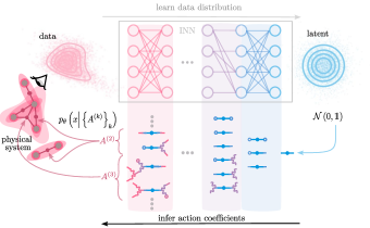
FIG. 1: Learning actions from data. We observe a physical system of interacting degrees of freedom (gray dots), whose precise interactions are unknown (shaded areas). We train a neural network on measurements of the system. The network learns in unsupervised fashion an estimate of the distribution of training data. We extract the action from the network parameters layer by layer, using a diagrammatic language. The final action coefficients $A^{(k)}$ represent the learned interactions (pink nodes).

II Actions in Physics

Physical theories are often formulated in terms of microscopic interactions of many constituents, the degrees of freedom $\left\{x_{i}\right\}_{1\leq i\leq d}$, where $d$ is the number of constituents and $x$ describes the system’s state. The degrees of freedom $\left\{x_{i}\right\}_{1\leq i\leq d}$ can be Ising spins, firing rates of neurons, social agents, or field points. The interactions of the constituents provide a mechanistic understanding of the system. The energy or Hamiltonian $H$ of the system can be written as the sum of these interactions. One can then ask how probable it is to observe the system in a specific microscopic state $x$ given an average energy $\langle H\rangle$. The most unbiased (maximum entropy) estimate of the probability density is then

$$p_{X}(x)=\frac{1}{Z}e^{-\beta H(x)}\,,$$

with $Z$ the normalization factor or partition function. Here $p_{X}$ is also known as the Boltzmann distribution [35]. In statistical physics, the prefactor $\beta$ is identified as the inverse temperature.

The action $S_{X}$ of this system is defined as the log probability, hence $S_{X}(x)=\ln\,p_{X}(x)=-\beta H(x)-\text{$\ln$}Z$. Therefore the system is fully characterized by $S_{X}$ and measurements of the system state $x$ correspond to drawing samples from $p_{X}$. Furthermore, up to the constant prefactor $-\beta$ and the constant $\text{$\ln$}Z$, the terms in the action are the same interaction terms as those in the Hamiltonian.

Consider an action of the form

$$S_{X}(x)= \,A^{(0)}+\sum_{i=1}^{d}A_{i}^{(1)}\,x_{i}+\sum_{i,j=1}^{d}A_{ij}^{(2)}\,x_{i}x_{j}$$

$$+\sum_{i,j,k=1}^{d}A_{ijk}^{(3)}\,x_{i}x_{j}x_{k}+\dots\,,$$ (1)

where the coefficients $A^{(k)}$ are tensors of rank $k$ and dimension $d$. Without loss of generality we choose the $A^{(k)}$ to be symmetric tensors, $A_{i_{1}\dots i_{k}}^{(k)}=A_{\mathcal{P}(i_{1},\dots,i_{k})}^{(k)}$ for any permutation $\mathcal{P}$ of the indices. These coefficients encode the coordination between the different degrees of freedom $x_{i}$. In general, we refer to a term of type $A_{i_{1},\dots,i_{k}}^{(k)}\,x_{i_{1}}\cdots x_{i_{k}}$, as a $k$-point interaction, since this term describes a coaction of $k$ degrees of freedom for $i_{1},\dots,i_{k}\in\left\{1,\dots,d\right\}$ all unequal. In this work, we focus exclusively on actions of the form of Eq. (1), which are suitable only for describing classical fields $x_{i}$, as the fields and the action coefficients are tensors and scalars, not operators. However, we are not limited to equilibrium statistical mechanics: the samples could as well stem from a time-dependent process; in this case, the action describes the measure on a path, which is allowed to come from a non-equilibrium system. Furthermore, even for quantum systems where the interactions are exactly known, a renormalized classical theory is sometimes sought to effectively describe the influence of quantum fluctuations [36, 37].

Notation

In the following, we use the notation $u^{\otimes k}$ for the outer product of $k$ instances of a tensor $u$

$$u^{\otimes k}=\underbrace{u\otimes u\otimes\cdots\otimes u}_{k\,\text{times}}\,,$$

and $T^{(k)}\cdot(u)^{\otimes l}$ for $l\leq k$ to denote the contraction of the first $l$ indices of a rank $k$ tensor $A^{(k)}$ with the first index of each tensor $u$:

$$\left(A^{(k)}\cdot(u)^{\otimes l}\right)_{\beta_{1},\dots\beta_{l},i_{l+1},\dots,i_{k}}=\sum_{i_{1},\dots,i_{l}}A_{i_{1},\dots,i_{k}}^{(k)}u_{i_{1}\beta_{1}}\cdots\,u_{i_{l}\beta_{l}},$$

with multi-indices $\beta_{1},\dots,\beta_{l}$ whose rank depends on the rank of $u$. In the special case that $u$ is a vector, the indices $\beta_{1},\dots,\beta_{l}$ vanish from the expression. If additionally $k=l$, the result is a scalar. Hence, Eq. (1) becomes

$$S_{X}(x)= \,A^{(0)}+A^{(1)}\cdot x+$$

$$\,A^{(2)}\cdot(x)^{\otimes 2}+A^{(3)}\cdot(x)^{\otimes 3}+\dots\,.$$

We symmetrize a tensor by averaging over the set $\mathcal{P}(\alpha)$ of all permutations of the multi-index $\alpha$:

$$\left(\operatorname{sym}A^{(k)}\right)_{\alpha}=\left|\mathcal{P}(\alpha)\right|^{-1}\sum_{\pi\in\mathcal{P}(\alpha)}A_{\pi}^{(k)}\,;$$

this operation does not change the result of polynomial contractions: $A^{(k)}\cdot(x_{l})^{\otimes k}\equiv\bigl{(}\operatorname{sym}A^{(k)}\bigr{)}\cdot(x_{l})^{\otimes k}$.

A typical objective in statistical physics is understanding how the microscopic interactions $A^{(k)}$ determine the macroscopic properties of the system. In this work, we take a different approach: Given samples from a system with unknown microscopic properties, we extract the interactions. Generative models such as INNs are a powerful tool to approximate data distributions $p_{X}$ [9, 10, 38, 13]. In the next section, we demonstrate how we can extract the interaction coefficients $A^{(k)}$ from trained networks.

III Learning Actions with Invertible Neural Networks

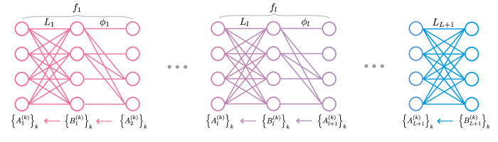
FIG. 2: Architecture and coefficient order. Invertible network composed of multiple layers. $L_{1},\ldots,L_{L+1}$ denote linear fully connected layers, $\phi_{1},\ldots,\phi_{L}$ are quadratic nonlinear activation functions. Coefficients $B_{l}^{(k)}$ of the action $S_{H,l}$ of pre–activations $h_{l}$ in layer $l$ of order $k$; coefficients $A_{l}^{(k)}$ of the action $S_{X,l}$ prior to linear layer $l$ of order $k$.

Invertible neural networks are used to learn the data distribution $p_{X}$ from a data set $\mathcal{D}$ of training samples [9]. They implement a bijective mapping $f_{\theta}:\mathbb{R}^{d}\rightarrow\mathbb{R}^{d}$, where the network output $z=f_{\theta}(x)$ is often referred to as the latent variable. The parameters $\theta$ of the network are trained such that the latent variables follow a prescribed target distribution. We follow a common choice for this latent distribution as a set of $d$ uncorrelated centered Gaussian variables with unit variance [9]

$$p_{Z}(z)=\exp\left(-\frac{1}{2}z^{\mathrm{\mathrm{T}}}z-\frac{d}{2}\ln 2\pi\right),$$ (2)

where $z^{\mathrm{\mathrm{T}}}z=\sum_{i=1}^{d}z_{i}^{2}$ denotes the Euclidean scalar product. Given $p_{Z}$, the probability assigned to a specific input is given by the change of variables formula

$$p_{\theta}(x)=p_{Z}\left(f_{\theta}(x)\right)\left|\det J_{f_{\theta}}\left(x\right)\right|\,,$$ (3)

which depends only on the network mapping $f_{\theta}$ and its Jacobian $J_{f_{\theta}}$. The training objective is to minimize the negative log-likelihood

$$\mathcal{L}\left(\theta\right) =-\sum_{x\in\mathcal{D}}\ln p_{\theta}(x)$$

$$=-\sum_{x\in\mathcal{D}}S_{\theta}(x)\,,$$ (4)

where in the second line we used that $\ln\,p_{\theta}$ is precisely the action $S_{\text{$\theta$}}$ of the learned distribution.

In this manner, we optimize Eq. (3) to approximate the unknown underlying data distribution using stochastic gradient descent. Since the target distribution, Eq. (2) is a set of independent Gaussians, the mapping $f_{\theta}:x\mapsto z$ of the network aims to eliminate cross-correlations and higher order dependencies of the components of the latent. On the level of the action, this means that all $k$-point interactions with $k\geq 3$ between components of $z$ must vanish. In turn, the inverse mapping defines a generative process that induces interactions in the learned distribution from a non-interacting latent theory.

We now define the architecture that allows us to obtain a polynomial action $S_{\text{$\theta$}}$ from the network parameters $\theta$. The network is composed of multiple layers $l$; every layer mapping $f_{l,\theta}:\mathbb{R}^{d}\rightarrow\mathbb{R}^{d}$ is an invertible function. For each layer, we define an output action $S_{X,l+1}$, which transforms into the input action $S_{X,l}$ via the change of variables formula. Using Eq. (3) we compute the input action $S_{X,l}$ of each layer given the output action $S_{X,l+1}$

$$S_{X,l}\left(x_{l}\right)=S_{X,l+1}\left(f_{l}\left(x_{l}\right)\right)+\ln\left|\det J_{f_{l}}\left(x_{l}\right)\right|\,,$$ (5)

starting with the polynomial action of the latent variable $S_{Z}(y)=\ln p_{Z}(y)$. We construct all layer mappings $f_{l}$ such that a polynomial action $S_{X,l+1}$ generates a polynomial action $S_{X,l}$ in Eq. (5) and thus by induction we obtain a polynomial learned input action $S_{\theta}$.

Each layer mapping $f_{l}$ is composed of a linear mapping $L_{l}$ and a nonlinear mapping $\phi_{l}$:

$$f_{l}\left(x_{l}\right)=\phi_{l}\circ L_{l}\left(x_{l}\right)\,.$$ (6)

In the overall architecture, linear and nonlinear mappings are therefore stacked alternately (see Fig. 2). After the last nonlinear transform $\phi_{L}$, we add an additional linear transform $L_{L+1}$, such that the network architecture begins and ends with a linear transform.

The transform of the action via a single layer, Eq. (5), similarly decomposes into two steps, with $h_{l}=L_{l}(x_{l})$ the intermediate activation:

$$S_{H,l}\left(h_{l}\right) =S_{X,l+1}\left(\phi_{l}\left(h_{l}\right)\right)+\ln\left|\det J_{\phi_{l}}\left(h_{l}\right)\right|\,,$$ (7)

$$S_{X,l}\left(x_{l}\right) =S_{H,l}\left(L_{l}\left(x_{l}\right)\right)+\ln\left|\det J_{L_{l}}\left(x_{l}\right)\right|\,.$$ (8)

The transformations from $S_{X,l+1}$ to $S_{H,l}$, and from $S_{H,l}$ to $S_{X,l}$ are therefore determined by $\phi_{l}$ and $L_{l}$, respectively, which we express schematically as

$$S_{X,l+1}\xrightarrow{\phi_{l}}S_{H,l}\overset{L_{l}}{\longrightarrow}S_{X,l}\,.$$ (9)

The remainder of this section is concerned with expressing (9) in terms of transforms of the action coefficients.

Since the actions are polynomials, at each step we can write $S_{X,l},\,S_{H,l}$ in terms of coefficients $\left\{A_{l}^{(k)}\right\}_{k},\left\{B_{l}^{(k)}\right\}_{k}$:

$$S_{X,l}(x_{l}) =\sum_{k=0}^{K_{l}}A_{l}^{(k)}\cdot(x_{l})^{\otimes k}\,,$$ (10)

$$S_{H,l}(h_{l}) =\sum_{k=0}^{K_{l}}B_{l}^{(k)}\cdot(h_{l})^{\otimes k}\,,$$ (11)

where the sum runs over the ranks $k$ of the coefficient tensors. Here $K_{l}$ is the degree of the polynomial in $h_{l}$, which depends on the layer index $l$. We show in the following that the rank of the polynomial does not change between $S_{X,l}$ and $S_{H,l}$ in the latter step of Eq. (9). The coefficients further uniquely determine the action. Therefore Eq. (9) is equivalent to the coefficient mapping

$$\left\{A_{l+1}^{(k)}\right\}_{k}\overset{\phi_{l}}{\longrightarrow}\left\{B_{l}^{(k)}\right\}_{k}\overset{L_{l}}{\longrightarrow}\left\{A_{l}^{(k)}\right\}_{k}\,.$$ (12)

In Fig. 2 we illustrate the order in which the coefficients are transformed.

We now derive the recursive equations for the coefficient transforms, beginning with the linear mapping.

Linear mapping

The linear mapping is given by

$$h_{l}=L_{l}\left(x_{l}\right) =W_{l}x_{l}+b_{l}\,,$$ (13)

with $W_{l},b_{l}\in\theta$. Combining Eq. (8) and Eq. (11) yields

$$S_{X,l}(x_{l}) =\sum_{k}B_{l}^{(k)}\cdot(W_{l}x_{l}+b_{l})^{\otimes k}+\ln\left|\det W_{l}\right|\,.$$ (14)

We find the transformed coefficients $A_{l}^{(k)}$ by expanding Eq. (14) and ordering them by powers in $x_{l}$. Higher-rank coefficients of $S_{H,l}$ contribute to lower-rank coefficients of $S_{X,l}$ via the contraction with the bias $b_{l}$. All remaining indices of $B_{l}^{(k)}$ must then be contracted with the first index of $W_{l}$:

$$A_{l}^{(k)}= \left[\sum_{k^{\prime}=0}^{K_{l}-k}\,\binom{k+k^{\prime}}{k^{\prime}}\,B_{l}^{(k+k^{\prime})}\cdot(b_{l})^{\otimes k^{\prime}}\right]\cdot(W_{l})^{\otimes k}\,$$

$$+\delta_{k0}\ln|\det W_{l}|\,.$$ (15)

The combinatorial factor $\binom{k+k^{\prime}}{k^{\prime}}$ arises due to the symmetry of the coefficients $B^{(k)}$: since they are symmetric under permutations of the indices, we only need to fix the number of contractions $k^{\prime}$ with the bias term $b_{l}$ and count all $\binom{k+k^{\prime}}{k^{\prime}}$ possible combinations of $k^{\prime}$ indices in $B^{(k)}$. Since $L_{l}$ is linear, $S_{X,l}$ and $S_{H,l}$ both have the same rank $K_{l}$.

We illustrate Eq. (15) for the final linear mapping of the network, the first coefficient transform that starts on the known latent space coefficients $\left\{B_{L+1}^{(k)}\right\}_{k}$ (on the far right in Fig. 2). The action of the latent distribution given in Eq. (2) describes a centered Gaussian with unit covariance; its first three coefficients are therefore $B_{L+1}^{(0)}=-\frac{d}{2}\ln 2\pi$, $B_{L+1}^{(1)}=0$ and $B_{L+1}^{(2)}=-\frac{1}{2}\mathds{1}$, and all coefficients with rank $k\geq 3$ being zero.

The transformed zeroth-rank coefficient $A_{L+1}^{(0)}$, which ensures that the action stays normalized, reads

$$A_{L+1}^{(0)} =-\frac{d}{2}\ln 2\pi+B_{L+1}^{(2)}\cdot(b_{L+1})^{\otimes k}+\ln\left|\det W_{L+1}\right|$$

$$=-\frac{d}{2}\ln 2\pi-\frac{|b_{L+1}|^{2}}{2}+\ln\left|\det W_{L+1}\right|\,.$$ (16)

The bias in the linear mapping shifts the mean of the probability distribution, which is induced by the first-order coefficient

$$A_{L+1}^{(1)} =\left[\,\binom{2}{1}\,B_{L+1}^{(2)}\cdot(b_{L+1})^{\otimes 1}\right]\cdot(W_{L+1})^{\otimes 1}\,$$

$$=-W_{L+1}^{\mathrm{\mathrm{T}}}b_{L+1}\,.$$ (17)

The second-rank coefficient is transformed in accordance with the rotation and scaling of the space due to $W_{L+1}$:

$$A_{L+1}^{(2)} =-B_{L+1}^{(2)}\cdot(W_{L+1})^{\otimes 2}\,$$

$$=-\frac{1}{2}W_{L+1}^{\mathrm{\mathrm{T}}}W_{L+1}\,.$$ (18)

In the case of actions with higher-order interactions $k\geq 3$, the coefficient transform Eq. (15) requires the computation of many more terms. To simplify the coefficient transforms, we therefore employ a diagrammatic language. A common practice in statistical physics is to represent $k$-th order interactions as vertices with $k$ legs [35]. Accordingly, we here express tensors of rank $k$ as vertices with $k$ legs and the contraction between tensors by an attachment of legs. This facilitates the computation of combinatorial factors, which can be read off from the diagram topology. The diagrammatic representations of Eqs. (16), (17), and (18) read:

$$A^{(0)}_{L+1} =\vbox{\hbox{\includegraphics[scale={1}]{Figures/Diagrams/A_0.pdf}}}+\vbox{\hbox{\includegraphics[scale={1}]{Figures/Diagrams/A_2_with_two_biases.pdf}}}+\ln\left|\det W_{L+1}\right|$$ (19)

$$A^{(1)}_{L+1} =2\vbox{\hbox{\includegraphics[scale={1}]{Figures/Diagrams/A_2_with_one_bias.pdf}}}$$ (20)

$$A^{(2)}_{L+1} =\vbox{\hbox{\includegraphics[scale={1}]{Figures/Diagrams/A_2_extended_legs.pdf}}}$$ (21)

A complete presentation of the diagrammatic method is provided in Appendix A.

Nonlinear mapping

We follow Dinh et al. [9] to define an invertible nonlinear mapping: we split the activation vectors and activation functions into two halves, denoting them by $h_{l}=\begin{pmatrix}h_{l}^{1}\\ h_{l}^{2}\end{pmatrix}$ and $\phi_{l}=\begin{pmatrix}\phi_{l}^{1}\\ \phi_{l}^{2}\end{pmatrix}$. The first half is passed onto the next layer unchanged; we then add a nonlinear function $\tilde{\phi}\left(h_{l}^{1}\right)$ of the first half onto the second half

$$x_{l+1}=\phi_{l}(h_{l})=\begin{pmatrix}\phi_{l}^{1}(h_{l})\\ \phi_{l}^{2}(h_{l})\end{pmatrix}=\begin{pmatrix}h_{l}^{1}\\ h_{l}^{2}\end{pmatrix}+\begin{pmatrix}0\\ \tilde{\phi}_{l}(h_{l}^{1})\end{pmatrix}\,.$$ (22)

We choose a quadratic nonlinearity,

$$\tilde{\phi}_{l}(h_{l}^{1})=\tilde{\chi}_{l}\cdot(h_{l}^{1})^{\otimes 2}\,,$$ (23)

where $\tilde{\chi}_{l}\in\mathbb{R}^{\left\lfloor\frac{d}{2}\right\rfloor\times\left\lceil\frac{d}{2}\right\rceil\times\left\lceil\frac{d}{2}\right\rceil}$ is a third-order tensor whose coefficients are trained, $\tilde{\chi}_{l}\in\theta$. In the following, we will use a shorthand notation $\phi_{l}(h_{l})=h_{l}+\chi_{l}\cdot(h_{l})^{\otimes 2}$ with $\tilde{\chi}_{l}$ being the non-zero part of $\chi_{l}$.

Equation (23) is the most elementary nonlinearity which is compatible with a polynomial action. Through the composition of $L$ layer transforms $f_{l}$, the network mapping becomes a polynomial of order $2^{L+1}$. The advantage of decomposing such a transform in terms of multiple applications of Eqs. (13) and (22) is a particularly simple form of the update equations for the coefficients.

Splitting the nonlinear mapping (22) makes it trivially invertible

$$h_{l}=\phi_{l}^{-1}(x_{l+1})=\begin{pmatrix}x_{l+1}^{1}\\ x_{l+1}^{2}\end{pmatrix}-\begin{pmatrix}0\\ \tilde{\phi}_{l}(x_{l+1}^{1})\end{pmatrix}\,,$$ (24)

as one can observe by evaluating the composition of Eqs. (22) and (24) on an arbitrary vector $h_{l}$.

We compute the action $S_{H,l}$ from $S_{X,l+1}$ using Eq. (8). Since the Jacobian $J_{\phi,l}$ of $\phi_{l}$ is a triangular matrix with ones on the diagonal, we have $\ln\left|\det J_{\phi,l}\right|=\text{0}.$ Therefore, the transform of the action induced by $\phi_{l}$ is just the composition

$$S_{H,l}(h_{l}) =S_{X,l+1}\left(h_{l}+\chi_{l}\cdot\left(h_{l}\right)^{\otimes 2}\right)$$

$$=\sum_{k}A_{l+1}^{(k)}\cdot\left(h_{l}+\chi_{l}\cdot\left(h_{l}\right)^{\otimes 2}\right)^{\otimes k}\,.$$ (25)

Equation (25) yields a polynomial of order $K_{l}=2K_{l+1}$. We expand the products in Eq. (25) and reorder the terms to obtain the transform of the action coefficients. Since each factor of $\chi_{l}$ increases the rank of the resulting tensor by one, lower-order coefficients $A_{l+1}^{(k-k^{\prime})}$ contribute to the coefficient $B_{l}^{(k)}$ via

$$\binom{k-k^{\prime}}{k^{\prime}}\,A_{l+1}^{(k-k^{\prime})}\cdot(\chi_{l})^{\otimes k^{\prime}}\,,$$

with $k>k^{\prime}\geq 1$. Each contraction of $A_{l+1}^{(k-k^{\prime})}$ with $\chi_{l}$ consumes one index in $A_{l+1}^{(k-k^{\prime})}$ and the first index in $\chi_{l}$, but adds two indices to the resulting tensor. As a result, for each $\chi_{l}$ in the contraction, the rank is raised by one. Therefore $k^{\prime}$ factors of $\chi_{l}$ are needed to increase the rank from $k-k^{\prime}$ to $k$. The factor $\binom{k-k^{\prime}}{k^{\prime}}$ arises because there are $\binom{k-k^{\prime}}{k^{\prime}}$ ways of choosing $k^{\prime}$ of the $k-k^{\prime}$ indices of the tensor to which to contract the factors of $\chi_{l}$. However, contractions of this type are no longer symmetric tensors because the resulting $k$-th order tensor has $2k^{\prime}$ indices stemming from $\chi_{l}$ and the remaining ones from $A^{(l+1,k-k^{\prime})}$. To express this result as a symmetric tensor, we symmetrize the result. This yields

$$B_{l}^{(k\leq 1)} =A_{l+1}^{(k)}$$

$$B_{l}^{(k>1)} =\operatorname{sym}\sum_{k^{\prime}=0}^{k}\,\binom{k-k^{\prime}}{k^{\prime}}\,A_{l+1}^{(k-k^{\prime})}\cdot(\chi_{l})^{\otimes k^{\prime}}\,.$$ (26)

Diagramatically, the contraction with $\chi_{l}$ is represented by splitting the legs of a vertex. By counting the number of splits we can therefore infer the number of factors $\chi_{l}$ of any diagram. To illustrate this, we here show the mapping $\left\{A_{L+1}^{(k)}\right\}_{k}\overset{\phi_{L}}{\longrightarrow}\left\{B_{L}^{(k)}\right\}_{k}$, which generates interactions up to the fourth order. The zeroth- and first-rank coefficients remain unchanged $B_{L}^{(0)}=A_{L+1}^{(0)}$ and $B_{L}^{(1)}=A_{L+1}^{(1)}$, as the $A_{L+1}^{(0)}$ has no legs to split; the splitting of legs in $A_{L+1}^{(1)}$ gives a contribution to $B_{L}^{(2)}$:

$$B^{(2)}_{L}=$$

$$+2\vbox{\hbox{\includegraphics[scale={1}]{Figures/Diagrams/A_2_one_bias_one_chi.pdf}}}$$ (27)

This diagrammatic expression corresponds to

$$B_{L}^{(2)}= B_{L+1}^{(2)}\cdot\left(W_{L+1}\right)^{\otimes 2}$$

$$+\operatorname{sym}\left(\left[B_{L+1}^{(2)}\cdot b_{L+1}\right]\cdot W_{L+1}\right)\cdot\chi_{L}$$

No further diagrams are generated from $A_{L+1}^{(1)}$, as all legs are split. The higher-order interactions $B_{L}^{(3)},\,B_{L}^{(4)}$ emerge through the splitting of legs in $A_{L+1}^{(2)}$

$$B^{(3)}_{L}= \,\binom{2}{1}\vbox{\hbox{\includegraphics[scale={1}]{Figures/Diagrams/A_2_one_chi.pdf}}}\,,$$ (28)

$$B^{(4)}_{L}=$$ (29)

In tensor notation, the same expressions read

$$B_{L}^{(3)} =\,\binom{2}{1}\,\operatorname{sym}\left[B_{L+1}^{(3)}\cdot\left(W_{L+1}\right)^{\otimes 2}\right]\cdot\chi_{L}\,,$$

$$B_{L}^{(4)} =\,\operatorname{sym}\left[B_{L+1}^{(3)}\cdot\left(W_{L+1}\right)^{\otimes 2}\right]\cdot\left(\chi_{L}\right)^{\otimes 2}\,.$$

This exemplifies how the interactions are built hierarchically as further layer transforms contribute contractions with $W_{l\leq L}$, $b_{l\leq L}$ and $\chi_{l<L}$, to previous coefficients. See Appendix A for further details.

The degree $K_{l}$ of the action doubles with each layer, starting from the output action with degree two. Networks of depth $L$ thus generate actions of degree $2^{L+1}$. Through the composition of several nonlinear mappings like Eq. (22), the prefactors $\chi_{l}$ of later layers will be exponentiated alongside their activations. Increasing the number of layers will therefore generate terms of arbitrarily high degree in both $x$ and in the prefactors. For example, the contribution of $\chi_{1}$ to $x_{L}$ will be of order $(\chi_{1})^{2^{L-1}}$. As a result, large values in $\chi_{l}$ are unfavorable as they make the activations diverge. In practice, we find that the entries of the tensors $\chi_{l}$ of trained networks are typically small, $\left|\left(\chi_{l}\right)_{ijk}\right|\ll 1$.

We note that all coefficients with rank $k>2$ must contain at least $k-2$ factors of $\chi_{l}$, where the different factors in general originate from different layers. These terms of rank $k>2$ constitute the non-Gaussian part of the action. Therefore, for applications where the data can be described as a perturbed Gaussian, small entries in $\chi_{l}$ are sufficient. The higher the rank of the coefficient, the smaller its entries. Consequently, we place a cutoff of two on the number of factors of $\chi_{l}$ in the action coefficients, thus ignoring negligible contributions. This effectively imposes a maximum rank of $k=4$ onto the action coefficients.

Coefficients of high rank can be numerically intractable for large dimension $d$, as their size grows as $\mathcal{O}\left(d^{k}\right)$. To mitigate this, we make use of Eq. (23) to write the coefficients in a decomposed form, focusing on the most significant contributions, which speeds up the computations and allows for tractable reductions in the size of the stored tensors. We specify this decomposition in Appendix B.

We began this section by equating the transform of the action through the network to the transform of its coefficients, decomposed as alternating linear and nonlinear transforms. We then made these transforms explicit in Eqs. (15) and (26). Given a trained network, these expressions allow us to extract the learned action through the iterative application of the coefficient transforms from the last layer to the first. In this way, we can describe the data distribution constructively, by tracking how the latent distribution is transformed through successive network layers.

Equation (26) shows how higher-rank coefficients hierarchically emerge through repeated contractions with the parameters $\chi_{L},\dots,\chi_{1}$ of the nonlinear mappings and $W_{L},\dots,W_{1},b_{L},\dots,b_{1}$ of the linear mappings of different layers. In the data space, these coefficients correspond to interactions; therefore this approach establishes an explicit relation between network parameters $\theta$ and the characteristic properties of the learned distribution $p_{\theta}.$ In the next section, we test this method in several cases with known ground-truth distributions.

IV Experiments

In this section, we will test the learning of actions in three different settings. In Section IV.1, we use a randomly initialized teacher network to generate samples. The teacher network has the same architecture as the one described in Section III, enabling us to compute the ground truth action. In Section IV.2, the ground truth action coefficients themselves are generated randomly, leading to multimodal data distributions. Finally in Section IV.3, we study a physics-inspired model system with interactions on a square lattice of $d=10^{2}$ sites.

IV.1 In-class distributions

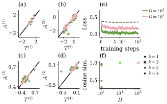
FIG. 3: Teacher-student coefficient comparison for varying training set sizes $D=|\mathcal{D}|$. Both teacher and student have depth $L=1$. (a–d) Student coefficients $A^{(k)}$ over teacher coefficients $T^{(k)}$ up to fourth order for $D=10^{3}$ in green and $D=10^{5}$ in pink. (e) Training loss (full lines) and test loss (dashed lines) over training steps. (f) Cosine similarity of coefficients over number of training samples.

First, we test whether we can recover the action coefficients of a known action from samples drawn from the respective distribution. We initialize a teacher network with random weights and compute the corresponding action coefficients $\left\{T^{(k)}\right\}_{k\leq 4}$ with the method outlined in Section III. We then generate a training set $\mathcal{D}$ by sampling Gaussian random variables $z\sim p_{Z}$ and apply the inverse network transform of the teacher on them; the elements of $\mathcal{D}$ are therefore samples from the teacher distribution. Since the teacher distribution is by construction part of the set of learnable student distributions, we refer to this as an in-class distribution. We then initialize a student network to identity $W_{l}=\mathds{1},\,b_{l}=0,\,\chi_{l}=0\,\forall l$ and train it on the training set $\mathcal{D}$. This choice for the initialization ensures that all variability in the trained result is due to the training data and the sequence of random batches drawn during training. After training, we extract the student coefficients $\left\{A^{(k)}\right\}_{k\leq 4}$ as described in Section III. The student network has learned the teacher distribution if the associated action coefficients match, $T^{(k)}=A^{(k)}\,\forall k$.

Note that $T^{(k)}=A^{(k)}\,\forall k$ does not imply that the parameters $\theta$ of the teacher and student network are equal. Due to the rotational invariance of the latent space, an additional linear transform which rotates the latent space $z$ does not result in a change in the learned action. Hence $T^{(k)}=A^{(k)}\,\forall k$ implies only that the two networks learn the same statistics.

We compare teacher and student coefficients in Fig. 3 for two different training set sizes $\left|\mathcal{D}\right|$. For a sufficiently large data set, the student can learn the teacher coefficients arbitrarily well: In Fig. 3 (a–d), the coefficient entries coincide while the network parameters $\theta$ do not align (see Appendix C for a comparison between network parameters). This confirms that the extracted coefficients are indeed characteristic of what the network has learned, as opposed to the parameters. Given sufficient samples, we therefore find that the method recovers the correct action coefficients.

For a smaller training set with $\lvert\mathcal{D}\rvert=10^{3}$, we find that the student network overfits the training set. To see this, we compute the test loss $\mathcal{L}_{\mathrm{test}}(\theta)$ on a test set of $10^{4}$ samples. In Fig. 3 (e) the test loss is significantly larger than the training loss. This is reflected in deviating coefficient entries in Fig. 3 (a–d). To quantify this disparity, we compute the cosine similarity between the tensors

$$\text{{\hbox{\cos\angle}}}\left(T^{(k)},S^{(k)}\right)=\frac{\left|\sum_{\alpha}T_{\alpha}^{(k)}S_{\alpha}^{(k)}\right|}{\sqrt{\sum_{\alpha}\left(S_{\alpha}^{(k)}\right)^{2}\sum_{\alpha}\left(T_{\alpha}^{(k)}\right)^{2}}}$$ (30)

where the sum runs over all independent indices $\alpha$, excluding duplicate tensors entries which are equal due to the symmetry. The cosine similarity ranges between zero and one, for perfect alignment it is equal to one. Fig. 3 (f) shows how the cosine similarity between teacher and student coefficients increases with the training set size. The lower order coefficients $T^{(k\leq 2)}$ are approximated well even in the case of little training data. The learned higher-order coefficients clearly deviate from the teacher coefficients in this case (see Fig. 3 (c,d,f)), indicating that the higher-order coefficients, corresponding to higher-order interactions in the teacher distribution, can only be conveyed through larger data sets.

Learning rules in coefficient space

Higher-order interactions depend on higher-order statistics of the data distribution, which must be expressed through a limited amount of samples. We train the network using stochastic gradient descent (SGD), which updates all parameters of the network at training time $t$ according to the dependence of the loss $\mathcal{L}$ on a subset of training data $\mathcal{D}_{t}\subset\mathcal{D}.$ In SGD, the update of a single weight $\Delta\theta_{i}=\theta_{i}(t+1)-\theta_{i}(t)$ is

$$\Delta\theta_{i} =-\eta\frac{\partial}{\partial\theta_{i}}\mathcal{L}_{\mathcal{D}_{t}}$$

$$=\eta\frac{\partial}{\partial\theta_{i}}\langle S_{\theta}(x)\rangle_{\mathcal{D}_{t}},$$ (31)

where $\eta$ is the learning rate and $\langle\cdot\rangle_{\mathcal{D}_{t}}$ denotes the average over the current training batch $\mathcal{D}_{t}$. In Appendix D, we show that this leads to a noisy update in the coefficients $A^{(k)}$ for $k\geq 1$ of

$$\Delta A_{\alpha}^{(k)}= \eta\left(\xi_{\alpha,t}^{(k)}+\bigl{\langle}\left(x^{\otimes k}\right)_{\alpha}\bigr{\rangle}_{\mathcal{D}}-\bigl{\langle}\left(x^{\otimes k}\right)_{\alpha}\bigr{\rangle}_{A}\right)\sum_{i}\left(\frac{\partial A_{\alpha}^{(k)}}{\partial\theta_{i}}\right)^{2}$$

$$+\eta\sum_{l,\alpha_{l}\neq\alpha}\left(\xi_{\alpha_{l},t}^{(l)}+\bigl{\langle}\left(x^{\otimes l}\right)_{\alpha_{l}}\bigr{\rangle}_{\mathcal{D}}-\bigl{\langle}\left(x^{\otimes l}\right)_{\alpha_{l}}\bigr{\rangle}_{A}\right)\sum_{i}\frac{\partial A_{\alpha}^{(k)}}{\partial\theta_{i}}\frac{\partial A_{\alpha_{l}}^{(l)}}{\partial\theta_{i}}+\mathcal{O}(\Delta\theta^{2})\,,$$ (32)

where $\langle\cdot\rangle_{\mathcal{D}}$ is the empirical average over all samples in the full training set $\mathcal{D}$, and $\langle\cdot\rangle_{A}$ is the expectation with regard to the current estimate of the density depending on learned coefficients $\left\{A^{(k)}\right\}_{k}$. The random variable $\xi_{t}^{(k)}$ encodes the difference between the mean estimated on the whole training set and a training batch. One can show that on average over all batches, the noise vanishes, $\langle\xi^{(k)}\rangle=0$ , and the variance also decreases with the training set size

$$\bigl{\langle}\!\bigl{\langle}\xi^{(k)}\bigr{\rangle}\!\bigr{\rangle}=\left(\bigl{\langle}x^{\otimes 2k}\bigr{\rangle}_{\mathcal{D}}-\left(\bigl{\langle}x^{\otimes k}\bigr{\rangle}_{\mathcal{D}}\right)^{\otimes 2}\right)|\mathcal{D}_{t}|^{-1}$$

(see e.g. [39]). Smaller batch sizes $|\mathcal{D}_{t}|$ therefore increase the noise in the updates of the action coefficients.

The expected update $\bigl{\langle}\text{$\Delta A_{\theta}^{(k)}\bigr{\rangle}$}$ vanishes on average over all batches when the learned moments and the moments on the training set match: $\langle x^{\otimes k}\rangle_{\mathcal{D}}=\langle x^{\otimes k}\rangle_{A}$. However, for any finite training set, there will furthermore be a deviation between $\langle x{}^{\otimes k}\rangle_{\mathcal{D}}$ and the true moment $\langle x{}^{\otimes k}\rangle_{T}$ of the teacher network. This expected difference scales as

$$\langle x{}^{\otimes k}\rangle_{\mathcal{D}}-\langle x{}^{\otimes k}\rangle_{T}\propto\sqrt{\left[\langle x{}^{\otimes 2k}\rangle_{T}-\left(\langle x{}^{\otimes k}\rangle_{T}\right)^{\otimes 2}\right]|\mathcal{D}|^{-1}}\,.$$

Therefore, not only will there be a batch-size dependent variability in the coefficient updates, but a bias induced by the limited amount of training data. This drift introduces a bias in the training, leading to overfitting. For many distributions, both $\langle x{}^{\otimes k}\rangle_{\mathcal{D}}-\langle x{}^{\otimes k}\rangle_{T}$ and $\langle\langle\xi^{(k)}\rangle\rangle$ increase with $k$ [40, 41]. In this case, both the bias and the variability of the training procedure increase with $k$, explaining why it is harder to learn higher-order statistics.

IV.2 Out-of-class distributions

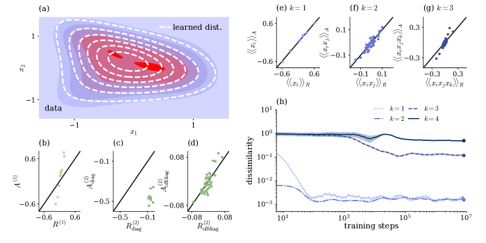
FIG. 4: Learning an effective monomodal theory. (a) Two-dimensional example of random density with multiple maxima. White lines are level lines of learned distribution for a five layer network. All other panels show results from a $d=10$-dimensional data set. (b–d) Learned over true coefficients for a three layer network on a $d=10$. We distinguish diagonal tensor entries from off-diagonal ones, where at least two indices differ. (e–g) Learned over true cumulants, computed from samples. Error bars are typically smaller than marker size. (h) Dissimilarity of true and learned cumulants: $1-\text{$\cos\angle$}\left(\langle\!\langle x^{\otimes k}\rangle\!\rangle_{A},\langle\!\langle x^{\otimes k}\rangle\!\rangle_{R}\right)$ over training steps. We record the cumulants at logarithmically spaced intervals during training. The curves are then smoothed by averaging over ten adjacent recording steps. Shaded areas show the variation due to the estimation of the cumulants from samples. Dots indicate training stage of cumulants shown in (e–g).

In the previous section, we have demonstrated that invertible networks accurately learn any distribution generated by the image set of inverse mappings $f_{\theta}^{-1}$. However, it is interesting to investigate how our approach deals with distributions outside this set. A first step to this end lies in understanding the nature of mappings employed by the invertible network.

The proposed network architecture belongs to the class of volume-preserving networks [9, 10]: the additive nature of the nonlinearity in Eq. (22) leads to a constant Jacobian determinant $\det J_{f_{\theta}}(x)$. The Jacobian determinant $\det J_{f_{\theta}}(x)$ of a mapping states how the image of the mapping is locally stretched. Since the only contribution to $\left|\det J_{f_{\theta}}(x)\right|$ comes from the linear transform, Eq. (13), the Jacobian determinant is constant. Therefore, this stretch is homogeneous everywhere. As a result, an invertible network with $\left|\det J_{f_{\theta}}(x)\right|=const.$ and a Gaussian target distribution $p_{Z}$ can only learn unimodal distributions $p_{\theta}$, i.e. distributions with only one maximum. To see this, we compute the gradient of Eq. (3) with respect to $x$:

$$\nabla_{x}p_{\theta}(x)=0\,\overset{\left|\det J_{f_{\theta}}(x)\right|=const.>0}{\Longleftrightarrow}\nabla_{f_{\theta}}p_{Z}\left(f_{\theta}(x)\right)=0\,.$$

This shows that the learned input distribution $p_{\theta}(x)$ has an extremum at $x_{0}$ if and only if the target distribution has an extremum at $f_{\theta}(x_{0})$. Since $p_{Z}$ has a single extremum, so does $p_{\theta}.$ This limitation is not unique to the choice of polynomial activations, but a consequence of the special structure of the Jacobian of the nonlinearity Eq. (22) and the latent distribution $p_{Z}$.

Since not every distribution is unimodal, we discuss in Section V how to extend the framework introduced here to incorporate multimodal distributions. An effective unimodal model, however, may also prove useful. While volume-preserving invertible networks with unimodal latent distribution $p_{Z}$ cannot learn a multimodal distribution $p_{\theta}$ exactly, they can learn an approximation. In this section we show how volume preserving networks can therefore be used to extract an effective theory in the multimodal case.

To avoid tieing results to a particular choice of distribution, we generate actions $S_{R}$ with random coefficients $\left\{R^{(k)}\right\}_{k\leq 3}$. A diagonal negative action coefficient $R^{(4)}$ is then added to obtain a normalizable distribution. We ensure that the corresponding distributions are multimodal and that their terms are balanced in strength using a sampling method for the coefficients that is detailed in Appendix E. Although the action $S_{R}$ is an unnormalized log-probability, we can then sample a training set $\mathcal{D}$ using Markov chain Monte Carlo; for this work we used a Hamiltonian Monte Carlo [42, 43, 44] sampler implemented in PyMC3 [45]. (For details see Appendix F.)

Given a known random action $S_{R}$ and a corresponding training set $\mathcal{D}$ of generated samples, we train networks of different depths and compare their action coefficients. In Fig. 4 (a) we show a two-dimensional example of such a randomly generated distribution as well as the learned monomodal approximation. Figure Fig. 4 (b)-(d) show comparisons of the true compared to the learned coefficients in the $d=10$ dimensional case. As expected, some action coefficients cannot be learned correctly. The largest deviations from the true coefficients occur in the diagonal entries $A_{i}^{(1)},A_{ii}^{(2)},\ldots$. However, we observe that many action coefficient entries that have at least two different indices (shown as $A_{\mathrm{offdiag.}}^{(2)}$in Fig. 4 (d)) recover approximately the correct value.

Using the network to generate samples, which hence belong to the learned distribution $p_{\theta}$, we compare the cumulants of the two distributions. The cumulants of a distribution can be computed from its moments and vice versa. For example, the first three cumulants are equal to the mean, the variance, and the centered third moment of a distribution. Cumulants are better suited than moments to compare two different distributions because they contain only independent statistical information. We distinguish $k$-th order cumulants from moments by using single brackets $\langle x^{k}\rangle$ for moments and double brackets $\langle\!\langle x^{k}\rangle\!\rangle$ for cumulants.

Despite the disparity in the coefficients, we find that the cumulants agree up to third order (compare panels (e) - (g) in Fig. 4). The learned distribution is therefore an effective theory that reproduces the statistics of the system beyond the Gaussian order, since in a Gaussian model the third-order cumulants are zero. Equation (32) shows that the action coefficient $A^{(k)}$ converges in expectation either when the moments of the training set and the learned distribution coincide, $\langle x{}^{\otimes k}\rangle_{\mathcal{D}}=\langle x^{\otimes k}\rangle_{A}$, or when the network cannot tune the coefficients in the relevant direction. Therefore the training aims to match the moments $\langle x{}^{\otimes k}\rangle_{\mathcal{D}},\langle x^{\otimes k}\rangle_{A}$ (and thereby, the cumulants) within the bounds of the flexibility allowed by the network architecture. We find that the higher order cumulants are learned later in training (see Fig. 4(h)).

Mulitmodality often appears as a result of symmetry breaking. Consider the classical example of an Ising model [46]. The action of this system is symmetric under a global flipping of all spins. Below the critical temperature, two modes appear, one for positive and one for negative net magnetization. However, in a physical system, this multimodality cannot be observed, because the probability of a global sign flip approaches zero as the system size increases. Furthermore, external factors such as coupling to the environment or a measurement device will also break the symmetry. In such a setting, the network can nevertheless find an informative theory, characterizing the observed monomodal distribution.

IV.3 Interaction on a lattice

Physical theories often feature a local structure of the interactions, for example, a lattice structure. We here construct such a system by introducing nearest-neighbor couplings on a square lattice of $d=10\times 10$ sites with periodic boundary conditions. Furthermore, we introduce self-interaction terms of second and fourth order. The resulting action is symmetric under a global sign change and under translations along the lattice. In an experiment, such symmetries may be broken by the coupling of the system to an external environment. We model this breaking of both symmetries by introducing a heterogeneous external field which introduces a bias to each degree of freedom.

The action therefore reads

$$S_{I} (x)=-\beta\left[\frac{1}{2}\sum_{i,j}x_{i}\left(r_{0}\delta_{ij}-\Lambda_{ij}\right)x_{j}+\sum_{i}\left(h_{i}x_{i}+ux_{i}^{4}\right)\right]\,$$

$$=:I^{(1)}\cdot x+I^{(2)}\cdot\left(x\right)^{\otimes 2}+I^{(4)}\cdot\left(x\right)^{\otimes 4}\,,$$ (33)

where the $I^{(k)}$ are the coefficients of the true distribution and we have omitted the normalization. Here $\beta$ serves as an inverse temperature. The matrix Laplacian $\Lambda_{ij}=-\delta_{ij}\text{deg}(i)+a_{ij}$ with $a_{ij}$ the adjacency matrix ($a_{ij}=1$ if $i,j$ are connected and $a_{ij}=0$ else) constitutes an interaction with the $\deg(i)=4$ nearest neighbors on the lattice. Both the diagonal part of $\Lambda$ and $r_{0}$ encode a second-order self-interaction.

The fourth-order term is another self-interaction $-\beta ux_{i}^{4}$. This model can be considered the lattice version of the effective long distance theory of an Ising model in two dimensions [46]. We illustrate the network topology and external field in Fig. 4(a).

As in Section IV.2, we sample from this distribution using an MCMC sampler (see Appendix F for details) and train networks of different depths $L$. In Fig. 5 (b-d) we compare the learned action coefficients $A^{(k)}$ to the corresponding target values $I^{(k)}.$ We find good agreement for $A^{(1)}$ and the off-diagonal values $A_{ij}^{(2)},i\neq j$, independent of network depth. The external field and nearest-neighbor coupling is therefore recovered accurately. The self-interaction $A_{\mathrm{diag}}^{(2)}$ is typically lower than the target value while the fourth-order self-interaction $A_{\mathrm{diag}}^{(4)}$ is typically larger. Since both parameters control the widths of the distributions, the slightly lower $A_{\mathrm{diag}}^{(2)}$ can compensate for the too small magnitude of $A_{\mathrm{diag}}^{(4)}$, producing an effective theory.

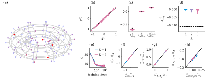
FIG. 5: Symmetry broken lattice model for networks of varying depth trained on a $d=10^{2}$ dimensional data set with $D=10^{6}$ samples. (a) Sites of square lattice with periodic boundary conditions distributed on a two-dimensional torus. Colored dots show strength of external field $h$ at connected lattice sites. (b) Learned over true first order coefficients for network depth $L=3$. (c) Distribution of learned coefficient entries $A^{(2)}$ compared to target values (black crosses) for network depth $L=3$. We distinguish self-interaction terms $A_{\mathrm{diag}}^{(2)}$ from off-diagonal entries $A_{\mathrm{offdiag}}^{(2)}$. From the off-diagonal entries $A_{\mathrm{offdiag}}^{(2)}$, we further separate those entries belonging to adjacent lattice sites $A_{\mathrm{offdiag}}^{(2),\mathrm{adj.}}$. (d) Training loss (solid curves) and test loss (dashed curves). Colors distinguish different network depths $L$. (e) Distribution of learned fourth order self-interactions as function of network depth. The dashed line marks the target value. (f–h) Learned over true cumulants of up to third order. Cumulants were computed on a subset of $10$ randomly chosen lattice sites. Colors distinguish different network depths $L$.

Nevertheless the higher-order coefficients $A^{(k\geq 3)}$ of the learned theory are relevant. We show in Fig. 5 (f-h), that the first, second, and third cumulants of the learned and true distribution approach each other as the network depth increases. A Gaussian approximation of $S_{I}$ would only tune $A^{(1)}$ and $A^{(2)}$ with $A^{(k\geq 3)}=0$ to match the first and second cumulants shown in Fig. 5 (f,g). As in the multimodal case therefore, we learn an effective non-Gaussian theory. The effective theory may result from the depth of the network being small in comparison to the dimensionality of the system to tune all higher order coefficients $A^{(k\geq 3)}$. The number of independent entries in the action coefficients up to the fourth order is $\mathcal{O}\left(d^{4}\right)$, roughly $4.6\cdot 10^{6}$ for the case of $d=10^{2}$, with by far the most number of entries in the highest-order coefficient $A^{(4)}.$ In contrast, the number of free parameters of a single layer is $\left\lceil\frac{d}{2}\right\rceil^{3}$ in $\tilde{\chi_{l}}$, $d^{2}$ in $W_{l}$, and $d$ in $b_{l}$, so all in all $\left\lceil\frac{d}{2}\right\rceil^{3}+d(d+1)$. Although the coefficients do not depend linearly on the network parameters, this gives a rough estimate of the required depth $L=34$ of the network, at which the number of free parameters in the network and in the coefficients coincide. Since the number of entries in the coefficients grows with $\mathcal{O}\left(d^{4}\right)$, but the number of free parameters in the network is only $\mathcal{O}\left(Ld^{3}\right)$, the depth required to tune all coefficient entries grows with $d$. Below this depth, it may well be that the flexibility of the network is too small to tune all fourth-order action coefficients. Even though $\bigl{\langle}\left(x^{\otimes k}\right)_{\alpha}\bigr{\rangle}_{\mathcal{D}}-\bigl{\langle}\left(x^{\otimes k}\right)_{\alpha}\bigr{\rangle}_{A}$ in Eq. (32) is likely non-zero then, the coefficients may still reach stationary values by the combination of the terms on the right hand side of Eq. (32) vanishing. Indeed we find in Appendix G, that in lower dimensions smaller network depths are sufficient to tune the higher statistical orders. Furthermore, the learned coefficients $A^{(4)}$ approach the target value as the depth increases. In all examples studied here, the alignment between learned and true statistics improves with depth, which increases the network flexibility. For shallow networks, however, although the learned action is not equal to the true one, it effectively describes the statistics of the true distribution beyond the Gaussian order as indicated by the good agreement of the cumulants. This behavior is equivalent to that of renormalized theories [46], which feature the same statistical correlations while changing the interaction strengths in a consistent manner.

V Discussion

We have developed a method to learn a microscopic theory from data – concretely, we learn a classical action that assigns a probability to each observed state. For this data-driven approach, we employ a specific class of deep neural networks that are invertible and that can be trained in an unsupervised manner, without the need of labeled training data. Such networks have been used before as generative models [9, 10, 13] but are generally considered a black box: after training the learned information is stored in a large number of parameters in an accessible, yet distributed and generally incomprehensible manner.

The diagrammatic formalism developed here allows us to extract the data statistics from the trained network in terms of an underlying set of interactions – a common formulation used throughout physics. To achieve this, we designed the network architecture as a trade-off between flexibility and analytical tractability. The choice of a quadratic polynomial, along with a volume-preserving invertible architecture, allows us to obtain explicit expressions for the interaction coefficients. This formalism shows how the interplay between linear and nonlinear mappings in the network composes non-Gaussian statistics, and hence higher-order interactions, in a hierarchical manner. As a consequence of the quadratic interaction constituting the fundamental building block, higher-order interactions are decomposed into this simplest possible form of nonlinear interplay. As a result, the order of interaction in the data directly maps to the required depth of the network in an understandable manner, thus providing an explanation why deep networks are required to learn higher-order interactions.

The analytical framework we developed can also readily be extended to higher-order nonlinearities: In terms of the diagrammatic language, the quadratic activations used in this work amount to splitting of “legs” in the Feynman diagrams into pairs. Likewise one obtains a three-fold splitting from a cubic term, a four-fold splitting from a quartic term and so on. Such higher-order nonlinearities would allow the building of more complex interactions with fewer layers.

From a physics point of view one may regard the trained network as a device to solve an interacting classical field theory in a data-driven manner: once the network has been trained, it maps each configuration of the interacting theory in data space to samples in latent space that follow a Gaussian theory, hence a non-interacting one. Such a mapping allows one to compute arbitrary connected correlation functions of the interacting theory. The framework offers two routes to this end. The traditional one uses common rules of diagrammatic perturbation theory to obtain controlled approximations of connected correlation functions in terms of connected diagrams constructed from propagators and interaction vertices of the inferred action. An alternative one directly constructs connected correlation functions hierarchically across the layers of the network, ultimately reduced to pairwise interactions on the level of the latent Gaussian. For example, the second order correlations read $\langle\!\langle x_{i}x_{j}\rangle\!\rangle_{p_{\theta}}=\langle\!\langle f_{\theta,i}^{-1}(z)f_{\theta,j}^{-1}(z)\rangle\!\rangle_{z\sim\mathcal{N}(0,\mathds{1})}$. For the n-th order correlations $\langle\!\langle x_{i_{1}}\cdots x_{n}\rangle\!\rangle_{p_{\theta}}$ one can therefore either work out the coefficients of the polynomial $f_{\theta,i_{1}}^{-1}(z)\cdots f_{\theta,i_{n}}^{-1}(z)$, in a similar manner to the action transform, and then average the resulting function over $p_{Z},$ or estimate the correlations by drawing samples from the generative network. An open avenue to explore further in this regard is the link between the presented framework and asymptotically free theories, where an interacting theory becomes non-interacting at high energy (UV) scales. In that case, different scales are connected by a renormalization group (RG) flow. It would be interesting to investigate whether the change of couplings described by the RG flow can be related to the transformations performed by the network. More broadly, the ability to learn an interacting theory by the network can be considered an alternative to asymptotic freedom, as the flow across layers does not have to correspond to a change of length scale.

To provide the most transparent setting, we have here chosen the simplest but common case of a latent Gaussian distribution, which has the aforementioned advantage of mapping to a non-interacting theory. A consequence is that the latent distribution only has a single maximum. Since for invertible volume-preserving networks the number of modes in data space and in latent space are identical, these network architectures therefore only learn monomodal distributions. For many settings of interest this is sufficient: multi-modal distributions in physical systems often occur together with non-ergodic behavior such as spontaneous symmetry breaking, selecting one of the modes of the distribution. As presented, our approach necessarily learns the statistics of the selected mode, and thus obtains an effective theory of the single selected phase of the system. The simplest way to learn genuine multi-modal distributions is the use of a multi-modal latent distribution, such as a Gaussian mixture. Our framework would then provide one set of action coefficient for each mixture component, correspondingly offering one effective theory for each phase.

We complement this study with a characterization of the training process, confirming the expectation that both larger training set size and network depth improve learning. Larger data sets in general decrease the bias of the learned distribution due to undersampling of the true distribution. This point is most severe for higher-order statistics, while the first two orders of the statistics are typically learned robustly also from limited data. We provide an approximate expression, Eq. (32), to investigate the convergence properties of statistics of different orders. While deeper networks are required to offer sufficient flexibility to learn higher-order statistics, the larger number of trainable parameters at the same time requires more to learn the statistics accurately. Alternatively, the network flexibility can be increased by raising the order of the polynomial activation function. Finding the optimal tradeoff between local nonlinearity and depth is an interesting point of future research.

Several studies have highlighted the role of the stochasticity of the training algorithm for networks performing classification [47, 48, 49]. A possible starting point to understanding SGD for generative models could be Eq. (32), which relates the trajectory of the learned distribution in coefficient space to the training algorithm. Equation (32) closely resembles the training of Restricted Boltzmann machines (RBMs), where the pairwise coupling matrix between hidden and visible layers updated according to the difference between learned and observed pairwise correlations [23]. Studying Eq. (32) could shed light on the dynamics of unsupervised learning, for which the architecture used in this work is a fully tractable prototype.

Another challenge in learning interacting theories of higher order is the necessarily large size of the action coefficients which grows with the dimension, irrespective of the manner in which these interactions are inferred. However, it is plausible that not all terms in these tensors are equally important: For spatially or temporally extended systems, interactions between distant degrees of freedom may be irrelevant. The framework explicitly shows how higher-order interactions are composed out of lower-rank coefficients. This may be leveraged to extract the most relevant contributions in a tractable manner (see Appendix B).

The general problem of inferring models from data discussed in this work is a well-known challenge. In the dynamical systems setting, the authors of [16, 17, 18, 50] use regression to infer the right hand side of the governing differential equation of a system from a set of basis functions. Other studies [14, 15] infer rules for the time-dependence of couplings (synaptic plasticity) using regression and genetic programming. These approaches produce interpretable models, but require a pre-determined a set of basis functions or operations, through the combination of which the system dynamics are approximated. Inference of parameters stochastic processes [19, 20, 21, 22] also relies on the specific form of the update equations. Prior knowledge about likely terms in the dynamical equations or their exact functional form is therefore needed in these works.

Many approaches exist to infer pair-wise couplings of binary degrees of freedom, such as for Ising models [46]. Prominent among them are Boltzmann machines [23]. Other techniques for Ising models first solve the forward problem, namely the statistics given the couplings – using variations of mean-field theory [24, 25, 26] or the TAP equations [51, 52, 27] – and then invert these relations explicitly or iteratively [53, 28, 29, 27]. Maximum likelihood methods or the TAP equations have also been used to infer the patterns of Hopfield models [30, 31]. In the special case of a tree-like, known network topology, or translationally invariant higher-order couplings along a linear chain, the inverse problem can be solved exactly [34]. Further works maximize the likelihood of the network model given the data, by using belief propagation to reconstruct the network structure from infection cascades [32], or Monte Carlo sampling to infer amino acid sequences in proteins [54]. In contrast to these works, in this study we consider continuous rather than discrete variables. Furthermore, we are not restricted to pairwise interactions and do not require prior knowledge on the structure of interactions.

Zache et al. [33] also solve the forward problem: they approximate a higher-order interacting theory to tree-level or one-loop-order in the effective action, and thereby obtain an invertible relation between interactions and correlations. This approach relies on the validity of the approximations, namely for the typically difficult step from interactions to correlation functions. These approximations are not necessary to train INNs, as the correlation functions are implicitly generated by the network mapping.

Neural networks have also previously been used to treat inverse problems. They are trained to infer the posterior probability of characteristic parameters given data [55, 56], and to compute renormalized degrees of freedom that are maximally informative about the global state of a system [57]. For systems of interacting identical particles, Cranmer et al. [58] use symbolic regression on trained Graphical Neural Networks to derive interpretable interactions. However, these approaches make no lucid connection between the learned model and the parameters of the neural network as we do in this study.

With the here proposed extraction method for the action of a physical system at hand, one can now proceed to extract hitherto unknown interacting models from data. One interesting application of this approach is to learn actions for systems for which a microscopic or mesoscopic description is not known, for example in biological neuronal networks: the inferred coefficients would determine the importance of nonlinear interactions in biological information processing. The approach may also be fruitful when applied to systems in physics where the microscopic theory may be known but an effective theory is sought that captures an observed macroscopic phenomenon.

APPENDIX A Diagrammatic update equations

We here describe the diagrammatic rules to compute the action coefficient transforms in Eqs. (15) and (26).

Following the structure in Section III, we first treat the linear transform (13). Each action coefficient $A_{l+1}^{(k)}$ is represented by a vertex, where the number of outgoing lines, also called legs, is equal to the rank of the coefficient. Each leg is assigned an index $i_{l}$ corresponding to the indices $(i_{1},\dots,i_{k})$ of the coefficient entry of $A_{l+1}^{(k)}$ it represents. Equation (15) shows that each index of the coefficient must either be contracted with $W_{l}$, and therefore remains a leg of the resulting vertex from the second index of $W_{l}$, or it must be contracted with $b_{l},$and therefore drops out. We represent the contraction with $W_{l}$ by an elongated line decorated with $W_{l}$, and the contraction with $b_{l}$ as a leg ending on an empty circle. Thus to compute the transformed action coefficients, we must add empty circles to the previous vertices in all possible ways and then elongate the remaining legs using $W_{l}$. A diagram with $k$ legs therefore produces the following diagrams:

$$\vbox{\hbox{\includegraphics[scale={1}]{Figures/Diagrams/LinearTransform.pdf}}}\rightarrow \vbox{\hbox{\includegraphics[scale={1}]{Figures/Diagrams/LinearTransformRHS_1.pdf}}},\binom{k}{1}\vbox{\hbox{\includegraphics[scale={1}]{Figures/Diagrams/LinearTransformRHS_2.pdf}}},$$

$$\dots,\binom{k}{k}\vbox{\hbox{\includegraphics[scale={1}]{Figures/Diagrams/LinearTransformRHS_3.pdf}}}$$

where the combinatorial factors $\binom{k}{l}$ arise due to the different ways of choosing legs which are contracted with $b_{l}$. For example, there are $\binom{k}{1}=k$ ways of choosing a single leg from a vertex with $k$ legs which is then contracted with $b_{l}$. We first compute the new diagrams for all $k$, then sum up all diagrams that have equal numbers of legs to one coefficient. This illustrates how higher-order action coefficients, by the contraction of their indices with the biases, i.e. the attachment of empty circles to their legs, contribute to lower-order coefficients.

For the nonlinear transform, we have the opposite effect: each index in the coefficient either remains or is contracted with $\chi_{l}$, which increases the rank of the transformed diagram by one. Therefore either the legs of vertices remain as they are, or they must be split into two to signify the contraction with $\chi_{l}$, which increases the number of legs of the vertex by one. We keep the split legs distinguishable from threepoint vertices by using curved lines for the split legs and sum over all possible ways to split legs. A diagram with $k$ legs therefore produces the following diagrams:

$$\vbox{\hbox{\includegraphics[scale={1}]{Figures/Diagrams/NonLinearTransformLHS.pdf}}}\rightarrow \vbox{\hbox{\includegraphics[scale={1}]{Figures/Diagrams/NonLinearTransformLHS.pdf}}},\binom{k}{1}\vbox{\hbox{\includegraphics[scale={1}]{Figures/Diagrams/NonLinearTransformRHS_2.pdf}}}$$

$$\dots,\binom{k}{k}\vbox{\hbox{\includegraphics[scale={1}]{Figures/Diagrams/NonLinearTransformRHS_3.pdf}}}$$

Here, the combinatorial factors arise due to the number of ways in which to choose the split legs. The number of factors $\chi_{l}$ in any diagram can then be read off from the number of leg splits. As in the linear transform, to compute the transformed action coefficients of rank $k,$ we must therefore sum over all diagrams with equal numbers of legs. This illustrates how higher-order action coefficients arise through the splitting of legs by factors of $\chi_{l}$.

APPENDIX B Decomposed tensors

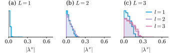
FIG. 6: Eigenvalue distributions of decomposed $\chi_{l}$ for networks of different depths. We decompose trained network parameters $\chi_{l}$ from Section IV.3 to the form of Eq. (35) and distinguish eigenvalues from the decomposed form of different layers $l$.

Higher-order tensors $T^{(k)}$ of rank $k$ can become numerically intractable for large dimension $d$ as the number of entries in $T^{(k)}$ grows as $\mathcal{O}\left(d^{k}\right)$. Specifically, two challenges arise: First, to store the entries of the tensors. Second, to compute contractions with matrices $W$ such as

$$T^{(k)}\cdot\left(W\right)^{\otimes k}\,,$$ (34)

which arise due to the linear coefficient transform Eq. (15). For these contractions, we must compute the sum over all entries

$$\left(T^{(k)}\cdot\left(W\right)^{\otimes k}\right)_{i_{{}^{1}}^{.},\dots i_{k}}=\sum_{j_{1},\dots j_{k}=1}^{d}T_{j_{1},\dots j_{k}}^{(k)}W_{j_{1},i_{1}}\cdots W_{j_{k},i_{k}}\,;$$

therefore without further simplification this entails the computation of $d^{k}$ entries of $T^{(k)}\cdot\left(W\right)^{\otimes k}$ from $d^{k}$ terms each, so the total number of floating point operations scales as $\mathcal{O}(d^{2k})$. Even though the number of steps required therefore only grows polynomially with $d$, for realistic data set sizes and $k=4$, this number increases very fast.

To facilitate the computation of coefficients with rank $k=4$, we exploit that they are built from coefficients of lower rank to write the tensors in a decomposed form.

As a first step, we decompose the network parameters $\chi_{l}$. Without loss of network expressivity, we may choose $\chi_{l}$ to be symmetric in its latter two indices $\left(\chi_{l}\right)_{\mu jk}=\left(\chi_{l}\right)_{\mu kj}$. In the following, we drop the layer index $l$ for brevity, as the structure of the computation is the same for any layer. We then rearrange the tensor to be a list of $d$ symmetric matrices $\bar{\beta}^{\mu},\,\mu=1,\dots,d$ such that $\chi_{\mu kj}=\bar{\beta}_{kj}^{\mu}$. Using the eigendecomposition of these matrices $\bar{\beta}^{\mu}$, we may write

$$\chi =\sum_{\mu,\nu=1}^{d}\gamma^{\mu,\nu}\otimes\beta^{\mu,\nu}\otimes\beta^{\mu,\nu}$$ (35)

where $\gamma^{\mu,\nu},\beta^{\nu}$ are vectors and $\gamma_{\tau}^{\mu,\nu}=\delta_{\tau,\mu}\lambda_{\nu}^{\mu}$ has only one non-zero entry, namely the $\nu$-th eigenvalue of the $\mu$-th matrix $\bar{\beta}^{\mu}$. To store this object we require $2d^{2}$ vectors of length $d$, namely $d^{2}$ vectors $\beta^{\mu,\nu}$ and $d^{2}$ vectors $\gamma^{\mu,\nu}$.The magnitude of entries in $\chi$ is directly related to the magnitude of the eigenvalues $\lambda_{\nu}^{\mu}$, which is typically small for trained networks. We show distributions of eigenvalues from trained networks in Fig. 6. The distributions broaden with increasing depth, however the peak of the distribution remains at $\left|\lambda_{\nu}^{\mu}\right|=0$. It is therefore possible to reduce the space required to store $\chi$ and all tensors related to it by placing a cutoff $\bar{\lambda}\geq\text{0}$ on the eigenvalues, keeping only the $\bar{n}\leq d^{2}$ largest eigenvalues which have $\left|\lambda_{\nu}^{\mu}\right|\geq\text{$\bar{\lambda}$}$. Then the number of entries required to store $\chi$ scales as $\mathcal{O}\left(2\bar{n}d\right)$, as again we need $2\bar{n}$ vectors of length $d$ each. To further simplify the expression, we absorb the sum over $\mu,\,\nu$ into a single index $\tau=1,\dots,\bar{n}$.

An alternative way to achieve the decomposition of $\chi$ into a reduced number of components would be to use the decomposed form Eq. (35) directly during training and limit the number of independent vectors $\beta^{\tau}$. This approach effectively trades the network expressivity for the tractability of the action coefficient transforms.

In addition to reduced storage requirements, the decomposed form (35) also has the advantage is that the decomposition translates to all tensors computed via contraction with $\chi$, which is how higher order coefficients are originally generated (compare with Eq. (26)). The contraction between a rank $k$ symmetric tensor $T^{(k)}$ and $\chi$ is

$$T^{(k)}\cdot\chi=\sum_{\tau}\left(T^{(k)}\cdot\gamma^{\tau}\right)\otimes\beta^{\tau}\otimes\beta^{\tau}\,.$$

If $k=1$, the result is just a matrix. If $k=2$, then $T^{(k)}\cdot\gamma^{\tau}=:\alpha^{\tau}$ is a vector, therefore $T^{(k)}\cdot\chi$ can be written as a sum of outer products between three vectors. If $k=3,$ the result is a sum of outer products between a matrix $T^{(k)}\cdot\gamma^{\tau}=\bar{\alpha}^{\tau}$ and two vectors;

$$T^{(3)}\cdot\chi=\sum_{\tau}\bar{\alpha}^{\tau}\otimes\beta^{\tau}\otimes\beta^{\tau}\,.$$ (36)

The matrices$\bar{\alpha}^{\tau}$ are symmetric since

$$\bar{\alpha}_{ab}^{\tau}=\sum_{c}T_{abc}^{(k)}\gamma_{c}^{\tau}=\sum_{c}T_{bac}^{(k)}\gamma_{c}^{\tau}=\bar{\alpha}_{ba}^{\tau}\,.$$

The case $k\geq 4$ does not arise, as any coefficient with degree $k\geq 4$ must already contain at least two factors $\chi$.

To store the factors of Eq. (36)we therefore require $\bar{n}$ matrices $\bar{\alpha}^{\tau}$ and $\bar{n}$ vectors $\beta^{\tau}$. The number of matrix and vector entries required to store this object is therefore $\mathcal{O}\left(\bar{n}d^{2}\right)$. The contraction with matrices $W$ along all indices is

$$\left(T^{(3)}\cdot\chi\right)\cdot\left(W\right)^{\otimes 4}=\sum_{\tau}\left(W^{T}\bar{\alpha}^{\tau}W\right)\otimes\left(W^{T}\beta^{\tau}\right)\otimes\left(W^{T}\beta^{\tau}\right)\,,$$

which corresponds to $\bar{n}$ matrix-vector products $W^{T}\beta^{\tau}$ and $2\bar{n}$ matrix-matrix products for $\bar{\alpha}^{\tau}W$ and $W^{T}\left(\bar{\alpha}^{\tau}W\right)$. Each term in the matrix-matrix product is computed from $d$ terms, therefore the number of terms required to compute $W^{T}\bar{\alpha}^{\tau}W$ is $\mathcal{O}(2d^{\omega})$ with the matrix multiplication exponent $\omega$, which depends on the concrete algorithm used for matrix multiplication, e.g. $\omega\approx 2.8$ for the Strassen algorithm [59]. To evaluate the contraction, we therefore need to compute $\mathcal{O}($$2\bar{n}d^{\omega})$ terms. Even in the case of no cutoff $\bar{\lambda}=0\Rightarrow\bar{n}=d^{2}$, this approach significantly reduces the required computations compared to the naive implementation.

In [60] it was shown that the number of floating point operations needed to compute general contractions of the type of Eq. (34) can be reduced by exploiting the symmetry of the tensors. They propose a simple scheme to reduce the number of floating point operations (using $\omega=3)$ to roughly $\mathcal{O}(d^{k+1}),$ and a more complex structure of saving these tensors, which further speeds up the computations at the expense of storing more intermediate entries. In our experiments, we have used a maximal dimensionality of $d=10^{2}$ in Section IV.3 and no cutoff $\overline{\lambda}=0.$ In the absence of any cutoff, we find a scaling of our algorithm roughly equal to the simpler scheme proposed in [60]. The combination of a cutoff, more efficient storing of symmetric tensors as suggested in [60], or restricting the number of free components in $\chi$ directly, facilitates the extension of the coefficient transforms to higher dimension $d$.

APPENDIX C Dissimilarity of parameters

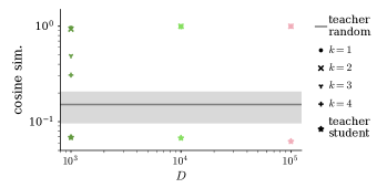
FIG. 7: Dissimilarity of parameters. Stars show the cosine similarities of the teacher and student network parameters trained on varying data set sizes $D$. The average cosine similarity between the teacher and $10^{2}$ randomly generated random networks is marked by the grey line, the shaded area encompasses one standard deviation. The remaining markers display the cosine similarity between the teacher coefficients $T^{(k)}$ and student coefficients $S^{(k)}.$

We here show that although the learned statistics of two networks may be the same, their parameters do not need to align. To this end, we use the teacher-student setup presented in Section IV.1, and compute the cosine similarities between pairs of network parameters $b_{l},\,W_{l},\,\chi_{l}$ – both between the teacher and the student, and between the teacher and a network of the same architecture with random Gaussian weights. We then average over the cosine similarities of the different parameters to obtain the average network cosine similarity. We show in Fig. 7 that although the teacher and student coefficients approach each other for increasing data set sizes $D$, their network parameters remain dissimilar. The appropriate object to compare the learned statistics is therefore the action, not the parameters of the network.

APPENDIX D Learning action coefficients with SGD

The learned action $S_{\theta}(x)$ depends on the parameters $\theta$ only through the coefficients $A^{(k)}$. We can therefore also view the training as a nonlinear optimization of the action coefficients via the parameters. However, we cannot freely move in this coefficient space: we must ensure that the action stays normalized, $\int\exp(S_{\theta}(x))dx=1$. To this end we fix the constant term in the action:

$$A^{(0)}=-\ln\int\exp\left(\sum_{k\geq 1}A^{(k)}\cdot\left(x\right)^{\otimes k}\right)dx\,.$$ (37)

Given this constraint, we rewrite the update equation (31) in terms of the coefficients using the chain rule,

$$\Delta\theta_{i}=\eta\sum_{k\geq 1}\sum_{\alpha_{k}}\frac{\partial}{\partial A_{\alpha_{k}}^{(k)}}\langle S_{\theta}(x)\rangle_{\mathcal{D}_{t}}\frac{\partial A_{\alpha_{k}}^{(k)}}{\partial\theta_{i}}\,,$$

where $\sum_{\alpha_{k}}$ runs over all possible (multi-)indices of $A^{(k)}.$ The update in the parameters induces a change in the action coefficients. We use this to approximate the update step for the coefficient entry $A_{\alpha}^{(k)}$ to linear order in the parameter updates:

$$\Delta A_{\alpha}^{(k)}\approx \sum_{i}\frac{\partial A_{\alpha}^{(k)}}{\partial\theta_{i}}\Delta\theta_{i}$$

$$= \eta\frac{\partial}{\partial A_{\alpha}^{(k)}}\langle S_{\theta}(x)\rangle_{\mathcal{D}_{t}}\sum_{i}\left(\frac{\partial A_{\alpha}^{(k)}}{\partial\theta_{i}}\right)^{2}$$

$$+\eta\sum_{l,\alpha_{l}\neq\alpha}\frac{\partial}{\partial A_{\alpha_{l}}^{(l)}}\langle S_{\theta}(x)\rangle_{\mathcal{D}_{t}}\sum_{i}\frac{\partial A_{\alpha}^{(k)}}{\partial\theta_{i}}\frac{\partial A_{\alpha_{l}}^{(l)}}{\partial\theta_{i}}\,.$$ (38)

The update step $\Delta A_{\alpha}^{(k)}$ therefore depends on the network architecture through the derivatives $\frac{\partial A_{\alpha}^{(k)}}{\partial\theta_{i}}$. The derivative of the expectation of the action with respect to the the coefficients in the former factor in Eq. (38) is

$$\frac{\partial}{\partial A_{\alpha}^{(k)}}\langle S_{\theta}(x)\rangle_{\mathcal{D}_{t}} =\langle\left(x^{\otimes k}\right)_{\alpha}\rangle_{\mathcal{D}_{t}}+\frac{\partial A^{(0)}}{\partial A_{\alpha}^{(k)}}$$

$$=\langle\left(x^{\otimes k}\right)_{\alpha}\rangle_{\mathcal{D}_{t}}-\langle\left(x^{\otimes k}\right)_{\underline{\alpha}}\rangle_{A},$$ (39)

where $\langle\cdot\rangle_{A}$ denotes the current average of the learned distribution and we used Eq. (37) in the second line. This term induces a variability in the coefficient updates, as $\langle x^{\otimes k}\rangle_{\mathcal{D}_{t}}$ will vary from batch to batch due to the finite size of each batch. We define the random variable $\xi_{t}^{(k)}=\langle x^{\otimes k}\rangle_{\mathcal{D}_{t}}-\langle x^{\otimes k}\rangle_{\mathcal{D}}$ to be the deviation between the moment estimated on the current batch $\mathcal{D}_{t}$ and the moment estimated on the entire data set $\mathcal{D}$. Combining Eqs. (39) and (38) yields Eq. (32).

APPENDIX E Random generation of multimodal actions(E)

Coefficient distributions for random actions

In section Section IV.2 we use multimodal actions $S_{R}$ constructed from randomly drawn coefficients $R^{(k)}$. A basic condition these coefficients must satisfy is that the resulting action be normalizable: $\int S_{R}(x)\,dx<\infty$. We note that for large enough $x$, the action is dominated by the highest order terms:

$$S(x)\xrightarrow[\lVert x\rVert\to\infty]{}\bigl{(}R^{(4)}\bigr{)}\cdot x^{\otimes 4}\,.$$

It is therefore necessary and sufficient for normalizability that $R^{(4)}$ be negative definite, which we ensure by choosing $R^{(4)}$ to be a diagonal tensor with negative coefficients:

$$R_{i_{1}i_{2}i_{3}i_{4}}^{(4)}=\begin{cases}-\frac{x_{r}^{-4}}{d}&\text{if }i_{1}=i_{2}=i_{3}=i_{4}\,;\\ 0&\text{otherwise}\,.\end{cases}$$ (40)

Here $d$ is the dimensionality of the data, and $x_{r}\in\mathbb{R}$ is a length scale which we are free to choose; one can view $R^{(4)}$ as a regulator term, and $x_{r}$ as the value for which it becomes strongly suppressing. For our experiments we used $x_{r}=1.0$.

Having ensured that the action is normalizable, we can define the probability $p_{R}(x\,|\,\{R^{(k)}\}_{k\leq 4})=\exp\bigl{(}S_{R}(x)\bigr{)}/\int\exp\bigl{(}S_{R}(x)\bigr{)}\,dx$ . We choose the $S_{R}$ such that the data can be described as a perturbation of a Gaussian theory — we therefore also choose $R^{(2)}$ to be negative definite (i.e. a valid precision matrix). Since any $d$-dimensional multivariate Gaussian can be written as a linear combination of $d$ independent Gaussian variables, we define $R^{(2)}$ as follows:

$$W_{ij} \sim\mathcal{N}(0,1/d^{2})\,, i,j =1,\dotsc d\,;$$

$$R_{ij}^{(2)} \coloneqq c-\frac{1}{2}\sum_{a}W_{ia}W_{ja}\,;$$ (41)

with $c=-0.1$ in our experiments. This is equivalent to transforming a Gaussian variable $z\sim\mathcal{N}(0,\mathds{1})$ by a linear transform $x=W^{-1}z$ and then computing the action of $x$ (compare to Eq. (18)).

Finally, the coefficients $R^{(1)}$ and $R^{(3)}$ are chosen as follows ($i,j,k=1,\dotsc d$):

$$R_{i}^{(1)} \sim\mathcal{N}\bigl{(}0,\sigma_{i}^{2}\bigr{)} \sigma_{i} =\frac{x_{r}^{-1}}{d}\,;$$

$$R_{ijk}^{(3)} \sim\mathcal{N}\bigl{(}0,\sigma_{ijk}^{2}\bigr{)} \sigma_{ijk} =\frac{x_{r}^{-3}}{s_{ijk}\gamma_{ijk}}\,.$$

The scaling with respect to $x_{r}^{-1}$ and $x_{r}^{-3}$ ensures that neither linear and cubic terms are negligible within the region where the regulator term $R^{(4)}$ is non-suppressing. The variable $\gamma_{\alpha}=\lvert\mathcal{P}(\alpha)\rvert$ in the denominator of $\sigma_{\alpha}$ is the multiplicity of the index $\alpha$. This is the number of times the component $R_{ijk}^{(3)}$ appears in $R^{(3)}$; since coefficients are symmetric, it is equal to the number of distinct permutations of $(i,j,k)$. We scale the multiplicity by $s_{\alpha}$, the number of different components which have the same number of permutations – for example the permutations of the indices $(2,1,1)$ and $(5,3,3)$ appear $\gamma_{ijj}=3$ times each, and there are $s_{ijj}=d(d-1)$ distinct entries of such indices. Scaling $\sigma_{\alpha}$ by $\gamma_{\alpha}$ and $s_{\alpha}$ ensures that both the on-diagonal and off-diagonal components of $R^{(2)},\,R^{(3)}$ are significant.

Multimodality of random actions

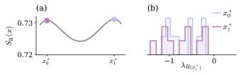
FIG. 8: Multiple local maxima in $S_{R}$. (a) $S_{R}$ along the straight line connecting two local maxima $x_{0}^{*},\,x_{1}^{*}$ of $S_{R}$ found by the optimization algorithm. (b,c)  Eigenvalues of the Hessian $H$ of $S_{R}$ at local maxima $x_{0}^{*},\,x_{1}^{*}$. All eigenvalues $\lambda_{H(x_{i}^{*})}$ are negative, therefore the action is convex down in all directions.

We here provide evidence that the distribution in Section IV.2 is indeed multimodal. To do so, we initialize an optimization algorithm at random points and attempt to find the maximum of $S_{R}(x^{*})$. We initialized at $10^{3}$ different values. In Fig. 8 we show the maximal values of $S_{R}(x^{*})$ found by the algorithm as well as the eigenvalues of the Hessian for selected, distinct final values $x^{*}$. Since all eigenvalues are below zero, the action $S_{R}$ is locally convex down in all directions at both points. The action $S_{R}$ therefore has at least two local maxima.

APPENDIX F Sampling actions with MCMC

Given ground truth coefficients $T^{(k)}$, we create a data set $\mathcal{D}$ by drawing samples according to the probability $p_{C}(x\,|\,\{T^{(k)}\}_{k\leq 4})$. Markov chain Monte Carlo (MCMC) is well suited to this task since it requires only the unnormalized log-probability, i.e. $S_{C}(x)$, and is guaranteed to converge to the true distribution (in contrast to variational methods like ADVI [61]). To generate $\mathcal{D}$, we used the No-U-Turn Sampler (NUTS) [62] implementation provided by PyMC3 [45]; sampler parameters mostly followed recommended defaults, with $10^{3}$ tuning steps and a mass matrix initialized to unity. The target acceptance rate was increased to $0.95$ to increase the sensitivity to small features of the probability distribution.

APPENDIX G Lattice model in low dimensions

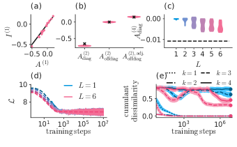
FIG. 9: Coefficients of lattice model for networks of varying depth trained on a $d=16$ dimensional data set with $D=10^{5}$ samples. (a) Learned ($L^{(1)})$ over true ($A^{(1)}$) first order coefficients. (b) Distribution of learned coefficient entries $A^{(2)}$ compared to target values (black crosses). Self-interaction terms are labeled $A_{\mathrm{diag}}^{(2)}$, off-diagonal entries $A_{\mathrm{offdiag}}^{(2)}$. Among the off-diagonal entries $A_{\mathrm{offdiag}}^{(2)}$, entries belonging to adjacent lattice sites $A_{\mathrm{offdiag}}^{(2),\mathrm{adj.}}$ are shown separately. (c) Training loss (full curves) and test loss (dashed curves). Colors distinguish different network depths $L$. (d) Distribution of learned fourth order self-interactions over network depth. The dashed line marks the target value. (e) Dissimilarity of true and learned cumulants: $1-\text{$\cos\angle$}\left(\langle\!\langle x^{\otimes k}\rangle\!\rangle_{A},\langle\!\langle x^{\otimes k}\rangle\!\rangle_{R}\right)$ over training steps. We record the cumulants at logarithmically spaced intervals during training. The curves are smoothed by averaging over ten adjacent recording steps. Shaded areas show the variation due to the estimation of the cumulants from samples. Dots indicate training stage of coefficients shown in (a,b).

We here show a lower dimensional version of the lattice model introduced in Section IV.3.

Here, the combined number of independent entries in the first four action coefficients is only $4844$, which corresponds to roughly $6$ network layers. Figure 9 shows a comparison of true vs. learned coefficients. Independent of network depth, we find that $A^{(1)}$ and the off-diagonal entries $A_{ij}^{(2)}$ with $i\neq j$ are recovered correctly (see Fig. 9 (a,b)). For shallow networks, the diagonal entries in the fourth order coefficient $A_{\mathrm{diag}}^{(4)}$ are approximately zero. Their magnitudes increase with $L$ (see Fig. 9 (d)). Increasing the depth $L$ also speeds up learning (see Fig. 9 (c)). Furthermore, we find that up to the fourth order, the cumulants of the learned distribution increasingly align with those of the true distribution as we increase network depth. Therefore we can conclude that increasing the depth of the network increases the accuracy of the learned distribution, both in terms of its coefficients and of its cumulants.

We repeated the experiment for $d=9$ without any heterogeneous external field, therefore $h=0$. Again, we find an alignment of most entries in $A^{(1)},A^{(2)},$with $A_{\mathrm{diag}}^{(2)}$ slightly lower than expected and $A_{\mathrm{diag}}^{(4)}$ larger than expected (see Fig. 10 (a,b)). In this setting, the symmetry of the action causes the first and third cumulant to vanish. We therefore only compute the alignment of the second and fourth cumulants. As in the previous cases, this alignment increases with depth, as shown in Fig. 10 (d). Therefore, the effective nature of the learned theory does not depend on the system’s symmetry being broken.

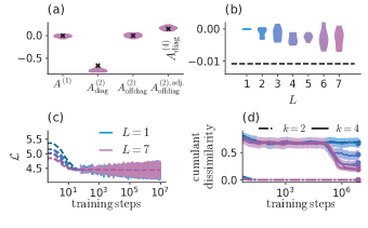
FIG. 10: Coefficients of lattice model without external field for networks of varying depth trained on a $d=9$ dimensional data set with $D=10^{5}$ samples. (a) Distribution of learned coefficient entries $A^{(1)},\,A^{(2)}$ compared to target values (black crosses). Self-interaction terms $A_{\mathrm{diag}}^{(2)}$ are shown separately from off-diagonal entries $A_{\mathrm{offdiag}}^{(2)}$. Among the off-diagonal entries $A_{\mathrm{offdiag}}^{(2)}$, those entries belonging to adjacent lattice sites $A_{\mathrm{offdiag}}^{(2),\mathrm{adj.}}$ are shown separately. (b) Distribution of learned fourth order self-interactions compared to network depth. The dashed line marks the target value. (c) Training loss (full curves) and test loss (dashed curves). Colors distinguish different network depths $L$. (d) Dissimilarity of true and learned cumulants: $1-\text{$\cos\angle$}\left(\langle\!\langle x^{\otimes k}\rangle\!\rangle_{A},\langle\!\langle x^{\otimes k}\rangle\!\rangle_{R}\right)$ over training steps. We record the cumulants at logarithmically spaced intervals during training. The curves are smoothed by averaging over ten adjacent recording steps. Shaded areas show the variation due to the estimation of the cumulants from samples. Dots indicate training stage of coefficients shown in (a,b).

References

- Lee and Jo [2022] S. Lee and J. Jo, Scale-invariant representation of machine learning, Physical Review E 105, 044306 (2022).
- Cohen et al. [2020] U. Cohen, S. Chung, D. D. Lee, and H. Sompolinsky, Separability and geometry of object manifolds in deep neural networks, Nature Communications 11, 746 (2020).
- Duranthon et al. [2021] O. Duranthon, M. Marsili, and R. Xie, Maximal relevance and optimal learning machines, Journal of Statistical Mechanics: Theory and Experiment 2021, 033409 (2021).
- Goldt et al. [2020] S. Goldt, M. Mézard, F. Krzakala, and L. Zdeborová, Modeling the influence of data structure on learning in neural networks: The hidden manifold model, Physical Review X 10, 041044 (2020).
- Refinetti et al. [2022] M. Refinetti, A. Ingrosso, and S. Goldt, Neural networks trained with SGD learn distributions of increasing complexity (2022), arxiv:arXiv:2211.11567 .
- Fischer et al. [2022] K. Fischer, A. René, C. Keup, M. Layer, D. Dahmen, and M. Helias, Decomposing neural networks as mappings of correlation functions (2022), arxiv:arXiv:2202.04925 .
- Tubiana and Monasson [2017] J. Tubiana and R. Monasson, Emergence of Compositional Representations in Restricted Boltzmann Machines, Physical Review Letters 118, 138301 (2017), arxiv:1611.06759 [cond-mat, physics:physics, stat] .
- Xiao and Pennington [2022] L. Xiao and J. Pennington, Synergy and Symmetry in Deep Learning: Interactions between the Data, Model, and Inference Algorithm, in Proceedings of the 39th International Conference on Machine Learning (PMLR, 2022) pp. 24347–24369.
- Dinh et al. [2014] L. Dinh, D. Krueger, and Y. Bengio, Nice: Non-linear independent components estimation, (2014), arXiv:1410.8516 .
- Dinh et al. [2017] L. Dinh, J. Sohl-Dickstein, and S. Bengio, Density estimation using Real NVP, arXiv:1605.08803 [cs, stat] (2017), arxiv:1605.08803 [cs, stat] .
- Ardizzone et al. [2019a] L. Ardizzone, J. Kruse, S. Wirkert, D. Rahner, E. W. Pellegrini, R. S. Klessen, L. Maier-Hein, C. Rother, and U. Köthe, Analyzing Inverse Problems with Invertible Neural Networks (2019a), arxiv:arXiv:1808.04730 .
- Odstrcil et al. [2022] R. E. Odstrcil, P. Dutta, and J. Liu, LINES: Log-Probability Estimation via Invertible Neural Networks for Enhanced Sampling, Journal of Chemical Theory and Computation 18, 6297 (2022).
- Kingma and Dhariwal [2018] D. P. Kingma and P. Dhariwal, Glow: Generative Flow with Invertible 1x1 Convolutions, in Advances in Neural Information Processing Systems, Vol. 31, edited by S. Bengio, H. Wallach, H. Larochelle, K. Grauman, N. Cesa-Bianchi, and R. Garnett (Curran Associates, Inc., 2018).
- Jordan et al. [2021] J. Jordan, M. Schmidt, W. Senn, and M. A. Petrovici, Evolving interpretable plasticity for spiking networks, eLife 10, e66273 (2021).
- Confavreux et al. [2020] B. Confavreux, F. Zenke, E. Agnes, T. Lillicrap, and T. Vogels, A meta-learning approach to (re)discover plasticity rules that carve a desired function into a neural network, in Advances in Neural Information Processing Systems, Vol. 33 (Curran Associates, Inc., 2020) pp. 16398–16408.
- Brunton et al. [2016] S. L. Brunton, J. L. Proctor, and J. N. Kutz, Discovering governing equations from data by sparse identification of nonlinear dynamical systems, Proceedings of the National Academy of Sciences 113, 3932 (2016).
- Casadiego et al. [2017] J. Casadiego, M. Nitzan, S. Hallerberg, and M. Timme, Model-free inference of direct network interactions from nonlinear collective dynamics, Nature Communications 8, 2192 (2017).
- Miller et al. [2020] J. Miller, S. Tang, M. Zhong, and M. Maggioni, Learning Theory for Inferring Interaction Kernels in Second-Order Interacting Agent Systems (2020), arxiv:arXiv:2010.03729 .
- Opper and Sanguinetti [2007] M. Opper and G. Sanguinetti, Variational inference for Markov jump processes, in Advances in Neural Information Processing Systems, Vol. 20 (Curran Associates, Inc., 2007).
- Opper [2019] M. Opper, Variational Inference for Stochastic Differential Equations, Annalen der Physik 531, 1800233 (2019).
- Vrettas et al. [2015] M. D. Vrettas, M. Opper, and D. Cornford, Variational mean-field algorithm for efficient inference in large systems of stochastic differential equations, Physical Review E 91, 012148 (2015).
- Ruttor and Opper [2009] A. Ruttor and M. Opper, Efficient Statistical Inference for Stochastic Reaction Processes, Physical Review Letters 103, 230601 (2009).
- Ackley et al. [1985] D. H. Ackley, G. E. Hinton, and T. J. Sejnowski, A learning algorithm for boltzmann machines, Cognitive Science 9, 147 (1985).
- Mezard and Sakellariou [2011] M. Mezard and J. Sakellariou, Exact mean field inference in asymmetric kinetic Ising systems, Journal of Statistical Mechanics: Theory and Experiment 2011, L07002 (2011), arxiv:1103.3433 [cond-mat] .
- Schneidman et al. [2006] E. Schneidman, M. J. Berry, R. Segev, and W. Bialek, Weak pairwise correlations imply strongly correlated network states in a neural population, Nature 440, 1007 (2006).
- Zeng et al. [2011a] H.-L. Zeng, E. Aurell, M. Alava, and H. Mahmoudi, Network inference using asynchronously updated kinetic Ising model, Physical Review E 83, 041135 (2011a).
- Sakellariou et al. [2012] J. Sakellariou, Y. Roudi, M. Mezard, and J. Hertz, Effect of coupling asymmetry on mean-field solutions of direct and inverse Sherrington-Kirkpatrick model, Philosophical Magazine 92, 272 (2012), arxiv:1106.0452 [cond-mat] .
- Roudi and Hertz [2011] Y. Roudi and J. Hertz, Mean field theory for nonequilibrium network reconstruction, 106, 048702 (2011).
- Baldassi et al. [2018] C. Baldassi, F. Gerace, L. Saglietti, and R. Zecchina, From inverse problems to learning: A Statistical Mechanics approach, Journal of Physics: Conference Series 955, 012001 (2018).
- Decelle et al. [2021] A. Decelle, S. Hwang, J. Rocchi, and D. Tantari, Inverse problems for structured datasets using parallel TAP equations and restricted Boltzmann machines, Scientific Reports 11, 19990 (2021).
- Cocco et al. [2011] S. Cocco, R. Monasson, and V. Sessak, High-dimensional inference with the generalized Hopfield model: Principal component analysis and corrections, Physical Review E 83, 051123 (2011).
- Braunstein et al. [2019] A. Braunstein, A. Ingrosso, and A. P. Muntoni, Network reconstruction from infection cascades, Journal of The Royal Society Interface 16, 20180844 (2019).
- Zache et al. [2020] T. V. Zache, T. Schweigler, S. Erne, J. Schmiedmayer, and J. Berges, Extracting the Field Theory Description of a Quantum Many-Body System from Experimental Data, Physical Review X 10, 011020 (2020).
- Mastromatteo [2012] I. Mastromatteo, Beyond Inverse Ising Model: Structure of the Analytical Solution, Journal of Statistical Physics 150, 10.1007/s10955-013-0707-y (2012).
- Goldenfeld [1992] N. Goldenfeld, Lectures on phase transitions and the renormalization group (Perseus books, Reading, Massachusetts, 1992).
- [36] S. Wessel, S. Trebst, and M. Troyer, A Renormalization Approach to Simulations of Quantum Effects in Nanoscale Magnetic Systems, MULTISCALE MODEL. SIMUL. 4, 237.
- Cuccoli et al. [1995] A. Cuccoli, R. Giachetti, V. Tognetti, R. Vaia, and P. Verrucchi, The effective potential and effective Hamiltonian in quantum statistical mechanics, Journal of Physics: Condensed Matter 7, 7891 (1995).
- Papamakarios et al. [2021] G. Papamakarios, E. Nalisnick, D. J. Rezende, S. Mohamed, and B. Lakshminarayanan, Normalizing flows for probabilistic modeling and inference, The Journal of Machine Learning Research 22, 57:2617 (2021).
- Cramér [1200] H. Cramér, Mathematical Methods of Statistics (PMS-9), Volume 9 (Mon, 04/12/1999 - 12:00).
- Krasilnikov et al. [2019] A. Krasilnikov, V. Beregun, and O. Harmash, Analysis of Estimation Errors of the Fifth and Sixth Order Cumulants, in 2019 IEEE 39th International Conference on Electronics and Nanotechnology (ELNANO) (2019) pp. 754–759.
- Beregun and Harmash [2018] V. Beregun and O. Harmash, Application of Cumulant Coefficients for Solving the Problems of Testing and Diagnostics in Control Systems, in 2018 IEEE 5th International Conference on Methods and Systems of Navigation and Motion Control (MSNMC) (2018) pp. 210–213.
- Duane et al. [1987] S. Duane, A. D. Kennedy, B. J. Pendleton, and D. Roweth, Hybrid Monte Carlo, Physics Letters B 195, 216 (1987).
- Neal [2012] R. M. Neal, MCMC using Hamiltonian dynamics, arXiv:1206.1901 [physics, stat] (2012), arxiv:1206.1901 [physics, stat] .
- Betancourt [2017] M. Betancourt, A Conceptual Introduction to Hamiltonian Monte Carlo, arXiv:1701.02434 [stat] (2017), arxiv:1701.02434 [stat] .
- Salvatier et al. [2016] J. Salvatier, T. V. Wiecki, and C. Fonnesbeck, Probabilistic programming in Python using PyMC3, PeerJ Computer Science 2, e55 (2016).
- Amit [1984] D. J. Amit, Field theory, the renormalization group, and critical phenomena (World Scientific, 1984).
- Li et al. [2017] Q. Li, C. Tai, and W. E, Stochastic Modified Equations and Adaptive Stochastic Gradient Algorithms, in Proceedings of the 34th International Conference on Machine Learning (PMLR, 2017) pp. 2101–2110.
- Chaudhari and Soatto [2018] P. Chaudhari and S. Soatto, Stochastic gradient descent performs variational inference, converges to limit cycles for deep networks (2018), arxiv:arXiv:1710.11029 .
- Mignacco et al. [2021] F. Mignacco, F. Krzakala, P. Urbani, and L. Zdeborová, Dynamical mean-field theory for stochastic gradient descent in Gaussian mixture classification*, Journal of Statistical Mechanics: Theory and Experiment 2021, 124008 (2021).
- Lu et al. [2019] F. Lu, M. Maggioni, and S. Tang, Learning interaction kernels in heterogeneous systems of agents from multiple trajectories, ArXiv (2019).
- Thouless et al. [1977] D. J. Thouless, P. W. Anderson, and R. G. Palmer, Solution of ’solvable model of a spin glass’, 35, 593 (1977).
- Vasiliev and Radzhabov [1974] A. N. Vasiliev and R. A. Radzhabov, Legendre transforms in the ising model, 21, 963 (1974).
- Zeng et al. [2011b] H.-L. Zeng, E. Aurell, M. Alava, and H. Mahmoudi, Network inference using asynchronously updated kinetic ising model, 83, 041135 (2011b).
- Mora et al. [2010] T. Mora, A. M. Walczak, W. Bialek, and C. G. Callan, Maximum entropy models for antibody diversity, Proceedings of the National Academy of Sciences 107, 5405 (2010).
- Gonçalves et al. [2020] P. J. Gonçalves, J.-M. Lueckmann, M. Deistler, M. Nonnenmacher, K. Öcal, G. Bassetto, C. Chintaluri, W. F. Podlaski, S. A. Haddad, T. P. Vogels, D. S. Greenberg, and J. H. Macke, Training deep neural density estimators to identify mechanistic models of neural dynamics, eLife 9, e56261 (2020).
- Ardizzone et al. [2019b] L. Ardizzone, J. Kruse, S. Wirkert, D. Rahner, E. W. Pellegrini, R. S. Klessen, L. Maier-Hein, C. Rother, and U. Köthe, Analyzing Inverse Problems with Invertible Neural Networks, arXiv:1808.04730 [cs, stat] (2019b), arxiv:1808.04730 [cs, stat] .
- Gökmen et al. [2021] D. E. Gökmen, Z. Ringel, S. D. Huber, and M. Koch-Janusz, Statistical physics through the lens of real-space mutual information, arXiv:2101.11633 [cond-mat] (2021), arxiv:2101.11633 [cond-mat] .
- Cranmer et al. [2020] M. Cranmer, A. Sanchez Gonzalez, P. Battaglia, R. Xu, K. Cranmer, D. Spergel, and S. Ho, Discovering symbolic models from deep learning with inductive biases, in Advances in Neural Information Processing Systems, Vol. 33, edited by H. Larochelle, M. Ranzato, R. Hadsell, M. Balcan, and H. Lin (Curran Associates, Inc., 2020) pp. 17429–17442.
- Strassen [1969] V. Strassen, Gaussian elimination is not optimal, Numerische Mathematik 13, 354 (1969).
- Schatz et al. [2014] M. D. Schatz, T. M. Low, R. A. van de Geijn, and T. G. Kolda, Exploiting Symmetry in Tensors for High Performance: Multiplication with Symmetric Tensors, SIAM Journal on Scientific Computing 36, C453 (2014).
- Kucukelbir et al. [2017] A. Kucukelbir, D. Tran, R. Ranganath, A. Gelman, and D. M. Blei, Automatic differentiation variational inference, Journal of Machine Learning Research 18, 1 (2017).
- Hoffman and Gelman [2014] M. D. Hoffman and A. Gelman, The No-U-turn sampler: Adaptively setting path lengths in Hamiltonian Monte Carlo., Journal of Machine Learning Research 15, 1593 (2014).