Stochastic Reachability of Discrete-Time Stochastic Systems via Probability Measures

Abstract

We develop a framework for stochastic reachability for discrete-time systems in terms of probability measures. We reframe the stochastic reachability problem in terms of reaching and avoiding known probability measures, and seek to characterize a) the initial set of distributions which satisfy the reachability specifications, and b) a Markov based feedback control that ensures these properties for a given initial distribution. That is, we seek to find a Markov feedback policy which ensures that the state probability measure reaches a target probability measure while avoiding an undesirable probability measure over a finite time horizon. We establish a backward recursion for propagation of state probability measures, as well as sufficient conditions for the existence of a Markov feedback policy via the 1-Wasserstein distance. Lastly, we characterize the set of initial distributions which satisfy the reachability specifications. We demonstrate our approach on an analytical example.

I Introduction

Stochastic reachability analysis is an established method for probabilistic safety, that provides an assurance that states that start within some initial set can reach a desired target set while avoiding a “bad” set, with at least some known likelihood. Such an assurance is important for stochastic dynamical systems in which satisfaction of state and input constraints is paramount, including problems in space vehicle rendezvous [1] and robotics [2, 3]. A theoretical foundation based in dynamic programming has been developed for stochastic reachability of discrete-time stochastic hybrid systems [4, 5]. However, the computational hurdles associated with dynamic programming are significant, as it requires gridding the state space and evaluating a value function at all points on the grid. Alternative approaches have been developed, based in abstraction [6], [7], sampling [8], and underapproximative methods [9] as well as approximative methods [10] in convex optimization.

Figure 1: Top: The standard stochastic reach-avoid problem finds the set of initial states for which there exists a Markov feedback policy that ensures that the state avoids an unsafe set (red) and reaches a target set (purple). Bottom: We re-frame the stochastic reach-avoid problem in terms of probability measures, to find the set of initial probability measures (orange) for which a Markov feedback policy ensures that the state probability measure avoids an unsafe probability measure (red) and reaches a desired target probability measure (purple) almost surely.

We propose an alternative technique for stochastic reachability that is based in probability measures. Probability measures can be used to represent not only the distributions of the state, but also whether a state lies within some region of interest. Probability measures have been employed in covariance steering [11, 12, 13] and distribution steering [14, 15] problems, in which the optimization problems minimize the distance between probability measures, as well as in data-driven reachability via Christoffel functions [16]. One advantage of employing probability measures is that we can exploit tools from measure theory to enforce guarantees that hold almost surely, meaning that properties over a probability measure hold with probability one. Further, recent work in optimal transport has yielded significant gains in computing with probability measures [17].

In this paper, we develop a theoretical foundation for propagation of probability measures that represent the distribution of the state of a discrete-time stochastic system over a finite horizon, and synthesize a Markov feedback policy that satisfies the reachability specifications. The Markov feedback policy minimizes the Wasserstein distance between distributions at each time step. In contrast to standard methods (Figure 1), which seek to synthesize the largest set of initial conditions which satisfy reachability specifications with at least a minimum likelihood, our approach assures reachability specifications almost surely. We obtain the set of initial probability measures, as well as a corresponding Markov feedback policy, in lieu of an initial set. Our approach is enabled by the representation of standard target and avoid sets as probability measures.

We describe mathematical preliminaries from probability and measure theory in Section II. In Section III, we describe the recursive evolution of probability measures over a finite-time horizon, presuming a known Markov feedback policy, and in Section IV we synthesize a controller which is assured to satisfy the reachability specifications almost surely. We demonstrate our approach on a small, analytic example in Section V, and conclude in Section VI.

II Preliminaries and Problem Formulation

Let $\mathbb{N}$ denote the natural numbers and $\mathbb{N}_{[a,b]}$ denote the set of natural numbers from $a$ to $b$ inclusively, for $a,b\in\mathbb{N}$ and $a\leq b$ [18]. Let $\mathbb{R}^{p}$ describe the extended real numbers $\mathbb{R}^{p}\cup\{-\infty,\infty\}^{p}$ of dimension $p\in\mathbb{N}$. Matrices and vectors are denoted with uppercase $D\in\mathbb{R}^{l\times p}$ and lowercase $d\in\mathbb{R}^{l}$, respectively. Random vectors are bolded, $\mathbf{y}\in\mathbb{R}^{p}$.

A probability space is a tuple $(\Omega,\mathscr{F},\mu)$, where $\Omega$ is the sample space and $\mathscr{F}$ is the $\sigma$-algebra containing measurable subsets of $\Omega$, i.e. events in the sample space, and a probability measure $\mu:\mathscr{F}\rightarrow[0,1]$. We consider the set of reals $\mathbb{R}^{p}$ that is separable and metrizable, that is, a Polish space [19, Conventions]. A continuous random vector $\mathbf{y}=[\mathbf{y}_{1}\cdots\mathbf{y}_{p}]^{\intercal}$ is a measurable function $\mathbf{y}:\Omega\rightarrow\mathbb{R}^{p}$ which maps from the probability space to a Borel measurable space $(\mathbb{R}^{p},\mathscr{B}(\mathbb{R}^{p}))$, where $\mathscr{B}(\mathbb{R}^{p})$ denotes the Borel $\sigma$-algebra and the inverse of the random vector is a subset of the $\sigma$-algebra, i.e., $\mathbf{y}^{-1}(\mathscr{B}(\mathbb{R}^{p}))=\{\omega:\omega\in\Omega,\mathbf{y}(\omega)\in\mathscr{B}(\mathbb{R}^{p})\}$.

Since we assume Borel measurable probability spaces on the set of reals, we utilize the cumulative distribution function (cdf) as the probability measure, $\mu_{\mathbf{y}}$, to define a probability space, $(\mathbb{R}^{p},\mathscr{B}(\mathbb{R}^{p}),\mu_{\mathbf{y}})$. The following Definition and Theorem establish this relationship.

Definition 1 (Cumulative Distribution Function [20, Sec. 6.3]).

A function $\Phi:\mathbb{R}^{p}\rightarrow[0,1]\subset\mathbb{R}$ is a cdf when it satisfies the following conditions:

1. The left and right limits of $\Phi$ are zero and one respectively, that is, $\lim_{y\rightarrow-\infty}\Phi(y_{1},\ldots,y_{p})=0$ and $\lim_{y\rightarrow\infty}\Phi(y_{1},\ldots,y_{p})=1$,

2. For a product of intervals, $\times_{i=1}^{p}(a_{i},b_{i}]\subset\mathbb{R}^{p}$, the mixed monotonicity of the function is non-negative, i.e.

   $$\Delta^{(a,b]}_{p}\Phi =\ \Phi(b_{1},\ldots,b_{p})$$

   $$\quad-\sum_{j=1}^{p}\Phi(b_{1},\ldots,b_{j-1},a_{j},b_{j+1},\ldots,b_{p})$$

   $$\quad+\sum_{1\leq j<k\leq p}\Phi(b_{1},\ldots,b_{j-1},a_{j},b_{j+1},\ldots,$$

   $$\hskip 100.00015ptb_{k-1},a_{k},b_{k+1},\ldots,b_{p})$$

   $$\quad+(-1)^{p}\Phi(a_{1},\ldots,a_{p})\geq 0$$ (1)

where $y=[y_{1}\cdots y_{p}]^{\intercal}\in\mathbb{R}^{p}$. Further, we denote for ease of notation $\Phi(y_{1},\ldots,y_{p})=\Phi(y)$.

Theorem 1 (Defining a cdf for a real random vector on a probability space).

For any random vector $\mathbf{y}$ on the probability space $(\mathbb{R}^{p},\mathscr{B}(\mathbb{R}^{p}),\mu_{\mathbf{y}})$, there exists a unique cdf, $\Phi_{\mathbf{y}}$, that satisfies Definition 1, where

$$\mu_{\mathbf{y}}((-\infty,y_{1}]\times\cdots\times(-\infty,y_{p}])$$ (2a)

$$=\mathbb{P}\{\mathbf{y}_{1}(\omega)\leq y_{1}\cap\cdots\cap\mathbf{y}_{p}(\omega)\leq y_{p}\}$$ (2b)

$$=\lim_{a\rightarrow\infty}\Delta^{(a,b]}_{p}\Phi_{\mathbf{y}}=\Phi_{\mathbf{y}}(y)$$ (2c)

Proof.

From [20, Sec. 6.1 and 6.3]. ∎

Since cdfs are unique, the converse of Theorem 1 allows one to define a random vector and its probability space, $(\mathbb{R}^{p},\mathscr{B}(\mathbb{R}^{p}),\mu_{\mathbf{y}})$, given a cdf.

Corollary 1 (Defining a probability space via cdf).

If a function $\Phi$ satisfies Definition 1, then there always exists a random vector $\mathbf{y}$ on a probability space $(\mathbb{R}^{p},\mathscr{B}(\mathbb{R}^{p}),\mu_{\mathbf{y}})$ such that $\Phi$ is its cdf, that is, $\Phi=\Phi_{\mathbf{y}}$.

Proof.

From [20, Sec. 6.1 and 6.3]. ∎

Thus, we can either define a random vector $\mathbf{y}$ such that there exists a corresponding cdf, $\Phi_{\mathbf{y}}(y)$, or define a cdf, $\Phi(y)$, such that it is the cdf of the random vector $\mathbf{y}$, that is, $\Phi_{\mathbf{y}}(y)=\Phi(y)$.

Finally, we say a function $g:\mathbb{R}^{p}\rightarrow\mathbb{R}^{l}$ is a Borel measurable function as long as it is continuous almost everywhere, meaning that continuity holds everywhere except a measurable subset of measure zero [21, Sec. 2.2].

II-A Discrete-time Stochastic Dynamical System

We define a discrete-time, stochastic system that evolves over a time horizon of $N$ steps, for time steps $k\in\mathbb{N}_{[0,N-1]}$.

Definition 2.

A discrete-time, stochastic system is a time-varying, Borel measurable mapping, $f_{k}:\mathbb{R}^{n}\times\mathcal{U}\times\mathcal{W}_{k}\rightarrow\mathbb{R}^{n}$,

$$x_{k+1} =f_{k}(x_{k},u_{k},w_{k})=[f_{1,k}(x_{k},u_{k},w_{k})\cdots$$

$$\hskip 100.00015ptf_{n,k}(x_{k},u_{k},w_{k})]^{\intercal},$$ (3)

where:

1. $\mathcal{U}\subseteq\mathbb{R}^{m}$ is the set of admissible inputs that is compact, where $u_{k}\in\mathcal{U}$ is the input vector.

2. $\mathcal{W}=\{(\mathcal{W}_{k},\mathscr{B}(\mathcal{W}_{k}))\}_{k=0}^{N-1}$, where $\mathcal{W}_{k}\subseteq\mathbb{R}^{p}$, is the set of Borel measurable spaces denoting the disturbance space, with random vector $\mathbf{w}_{k}$ on a probability space $(\mathcal{W}_{k},\mathscr{B}(\mathcal{W}_{k}),\mu_{\mathbf{w}_{k}})$ where $\Phi_{\mathbf{w}_{k}}(w_{k})$ is its cdf.

3. $\Phi_{\mathbf{x}_{k+1}}:\mathscr{B}(\mathbb{R}^{n})\times\mathbb{R}^{n}\times\mathbb{R}^{n}\times\mathcal{W}_{k}\times\mathcal{U}\rightarrow[0,1]$ is a cdf representing the time-varying transition kernel for a random vector $\mathbf{x}_{k+1}$ on the probability space $(\mathbb{R}^{n},\mathscr{B}(\mathbb{R}^{n}),\mu_{\mathbf{x}_{k+1}})$, given the current state $x_{k}\in\mathbb{R}^{n}$, disturbance $\mathbf{w}_{k}$, and input $u_{k}\in\mathcal{U}$.

We define the transition kernel in terms of the probability measure of the random vector $\mathbf{w}_{k}$ [22, Ch. 8],

$$\Phi_{\mathbf{x}_{k+1}}(x_{k+1},x_{k},u_{k})$$

$$=\mu_{\mathbf{w}}(\{x_{k+1}\in\mathbb{R}^{n}:f_{1,k}(x_{k},u_{k},\mathbf{w}_{k})\leq x_{1,k+1}\times$$

$$\hskip 49.79231pt\cdots\times f_{n,k}(x_{k},u_{k},\mathbf{w}_{k})\leq x_{n,k+1}\}|x_{k},u_{k})$$ (4a)

$$=\Phi_{f_{k}(x_{k},u_{k},\mathbf{w}_{k})}(x_{k+1},x_{k},u_{k}).$$ (4b)

We also presume a Markov feedback policy $\pi_{k}:\mathbb{R}^{n}\rightarrow\mathcal{U}$ that depends on the current state, $x_{k}$.

Definition 3 ([22, , Sec. 8.1, Def. 8.2]).

A Markov feedback policy is a sequence $\pi=\{\pi_{0},\ldots,\pi_{k},\ldots,\pi_{N-1}\}$ such that each Markov feedback map, $\pi_{k}:\mathbb{R}^{n}\rightarrow\mathcal{U}$ for $k\in\mathbb{N}_{[0,N-1]}$, is a time-varying, non-random, Borel measurable function, that is, $u_{k}=\pi_{k}(x_{k})$.

II-B Set Representations via Measure Theory

We use tools from measure theory to represent a change of measure and probabilities of a random vector $\mathbf{y}$ residing in a Borel measurable set via probability measures.

Theorem 2 (Radon-Nikodym Theorem, [20]).

If $\nu$ and $\mu$ are $\sigma-$finite measures (e.g., probability measures) on the Borel measurable space $(\mathbb{R}^{p},\mathscr{B}(\mathbb{R}^{p}))$, where $\mu$ is absolutely continuous with respect to $\nu$, that is, $\mu<<\nu$, then there exists a measurable function $g(y)\geq 0$ such that

$$\mu(G)=\int_{G}g(y)\mathrm{d}\nu(y),\ \forall G\in\mathscr{B}(\mathbb{R}^{p}).$$ (5)

The function $g(y)=\frac{\mathrm{d}\mu}{\mathrm{d}\nu}$ is the Radon-Nikodym derivative of $\mu$ with respect to $\nu$.

Theorem 2 imposes a change of measure via a non-negative measurable function. We make use of the the Dirac measure, a probability measure over a set, as such a non-negative measurable function.

Definition 4 (Dirac Measures [21, Sec. 1.3]).

Given a probability space $(\mathbb{R}^{n},\mathscr{B}(\mathbb{R}^{n}))$, a Dirac measure is $\delta_{y}:G\rightarrow\{0,1\}$ where

$$\delta_{y}(G)=\begin{cases}1,\ y\in\mathcal{G}\\ 0,\ y\notin\mathcal{G}\\ \end{cases}.$$ (6)

Note that the Dirac measure functions similarly to an indicator function ($\mathbb{1}_{G}(y)=1$ if $y\in G$, and is 0 otherwise).

Corollary 2 (Random Vector Residing in a Set via Dirac Measure).

Given the probability measure of a random vector residing within a set, $\mu(G)=\mathbb{P}\{\mathbf{y}\in G\}$, and the cdf of $\mathbf{y}$, $\Phi_{\mathbf{y}}$, such that $\mu(G)<<\Phi_{\mathbf{y}}$, then the Dirac measure of a point $y$ residing in a set, $\delta_{y}(G)$, is a non-negative measurable function such that

$$\mu(G)=\int_{\mathbb{R}^{p}}\delta_{y}(G)\mathrm{d}\Phi_{\mathbf{y}}(y).$$ (7)

Proof.

This follows directly from Theorem 2. ∎

II-C Problem Formulation

We seek to find the set of initial probability measures for which the state of the stochastic system in Definition 2, with some Markov feedback policy $\pi$, will satisfy

$$\mathbb{P}\left\{\mathbf{x}_{N}\in\mathcal{T}\cap\left(\cap_{k=0}^{N-1}\mathbf{x}_{k}\not\in\mathcal{A}\right)\right\}$$ (8)

almost surely. In words, we wish for the system to reside in a target region, $\mathcal{T}$, at final time $N$, while avoiding an unsafe region, $\mathcal{A}$, for $k\in\mathbb{N}_{[0,N-1]}$ with probability 1 almost everywhere. Equation (8) imposes reaching a target region, $\mathcal{T}$, while avoiding an undesired region, $\mathcal{A}$, by staying within a target tube that is its complement, $\mathcal{A}^{\complement}$ [9].

We first transform these set representations to probability measures of the target set and the target tube via Definition 4.

$$\mu_{\mathcal{T}}(x_{N}) =\delta_{x_{N}}(\mathcal{T})$$ (9a)

$$\mu_{\mathcal{A}^{\complement}}(x_{k}) =\delta_{x_{k}}(\mathcal{A}^{\complement})$$ (9b)

We encode the avoid probability measure in terms of its complement, $\mu_{\mathcal{A}}(x_{k})=1-\mu_{\mathcal{A}^{\complement}}(x_{k})$. Note that this transformation is readily extendable to random sets [23].

Problem 1 (Stochastic Reach-Avoid via Probability Measures).

Given a target probability measure, $\mu_{\mathcal{T}}$, and an avoid probability measure, $\mu_{\mathcal{A}}$, we seek to find $P_{\mathbf{x}_{0}}$, the set of initial probability measures, for which there exists a Markov feedback policy such that the probability measure of state of the system in Definition 2 reaches $\mu_{\mathcal{T}}$ at the final time $N$ and avoids $\mu_{\mathcal{A}}$ for all time steps $k\in\mathbb{N}_{[0,N-1]}$, almost surely.

We solve Problem 1 in two steps. First, in Section III, we presume that a Markov feedback policy exists and we recursively construct the state probability measures which satisfy the reach-avoid specifications almost surely backwards-in-time. Second, in Section IV, we construct Markov feedback policies for every initial probability measure that satisfies the reach-avoid specification almost surely, then construct the set of initial probability measures, $P_{\mathbf{x}_{0}}$.

III Backward Recursion of the State Probability Measure

We seek to characterize the backward recursion that enables propagation of probability measures (Figure 2) that satisfy the target and avoid probability measures. To do so, we first describe the state probability measure $\mathbf{x}_{k+1}$ in terms of the cdf of the prior state, $\mathbf{x}_{k}$, using the relationship in (4).

$$\Phi_{\mathbf{x}_{k+1}}(x_{k+1})$$

$$\hskip 30.00005pt=\int_{\mathbb{R}^{n}}\Phi_{f_{k}(x_{k},u_{k},\mathbf{w}_{k})}(x_{k+1},x_{k},\pi_{k}(x_{k}))\mathrm{d}\Phi_{\mathbf{x}_{k}}(x_{k})$$ (10)

Lemma 1 (Uniqueness of State Probability Measure at Time $k$).

For a probability measure $\Phi_{\mathbf{x}_{k+1}}$ and a known Markov feedback map $\pi_{k}(x_{k})$, there exists a unique probability measure $\Phi_{\mathbf{x}_{k}}$ such that (III) holds.

Proof.

From [21, Lemma 10.4.3]. ∎

Satisfaction of the avoid and target probability measures requires additional constraints to be placed on this propagation. To constrain the state probability measure $\Phi_{\mathbf{x}_{k}}$ so that it avoids the avoid probability measure $\mu_{\mathcal{A}}$, we seek to satisfy

$$\int_{\mathbb{R}^{n}}\mu_{\mathcal{A}^{\complement}}(x_{k})\mathrm{d}\Phi_{\mathbf{x}_{k}}(x_{k})=1.$$ (11)

This constraint arises from the definition of satisfaction of the target tube constraint almost surely.

For the state probability measure to meet the target set requirement, we must constrain $\Phi_{\mathbf{x}_{N-1}}$ as follows,

$$\int_{\mathbb{R}^{n}}\int_{\mathbb{R}^{n}}\mu_{\mathcal{T}}(x_{N})\mathrm{d}\Phi_{\mathbf{\hat{x}}_{N}}(x_{N},x_{N-1},\pi_{N-1}(x_{N-1}))$$

$$\hskip 110.00017pt\cdot\mathrm{d}\Phi_{\mathbf{x}_{N-1}}(x_{N-1})=1,$$ (12)

for $\mathbf{\hat{x}}_{N}=f_{N-1}(x_{N-1},u_{N-1},\mathbf{w}_{N-1})$. We formalize these notions in the following Theorem.

Figure 2: The backward recursion (III) and constraints (11), (III) together ensure that the target probability measure can be reached and the avoid probability measure avoided, subject to stochastic system dynamics and a known controller.

Theorem 3.

Given a target probability measure $\mu_{\mathcal{T}}$, a target tube probability measure $\mu_{\mathcal{A}^{\complement}}$, and a Markov feedback policy $\pi$, the state probability measure must satisfy (III) for $k\in\mathbb{N}_{[0,N-1]}$, as well as

1. (11) for $k\in\mathbb{N}_{[0,N-2]}$,

2. (III) for $k=N-1$,

in order to satisfy the reachability constraints almost surely.

Proof.

Consider the case in which $k=N-1$: Note that (III) holds as long as $\Phi_{\mathbf{x}_{N-1}}(x_{N-1})$ satisfies (11).

Now consider $k\in\mathbb{N}_{[0,N-2]}$. We employ backwards induction, beginning with the base case $k=N-2$,

$$\Phi_{\mathbf{x}_{N-1}}(x_{N-1})$$

$$=\int_{\mathbb{R}^{n}}\Phi_{f_{N-2}(x_{N-2},u_{N-2},\mathbf{w}_{N-2})}(x_{N-1},x_{N-2},\pi_{N-2}(x_{N-2}))$$

$$\hskip 140.00021pt\cdot\mathrm{d}\Phi_{\mathbf{x}_{N-2}}(x_{N-2}),$$ (13)

holds almost everywhere as long as $\Phi_{\mathbf{x}_{N-2}}(x_{N-2})$ satisfies (11). If the equality holds for the case $k=j$ where $j<N-2$, then it must also hold for the case $k=j-1$. Observe that for $k=j-1$ and $k=j$ the recursions, respectively,

$$\Phi_{\mathbf{x}_{j+1}}(x_{j+1})=\int_{\mathbb{R}^{n}}\Phi_{f_{j}(x_{j},u_{j},\mathbf{w}_{j})}(x_{j+1},x_{j},\pi_{j}(x_{j}))$$

$$\hskip 170.00026pt\cdot\mathrm{d}\Phi_{\mathbf{x}_{j}}(x_{j}$$ (14a)

$$\Phi_{\mathbf{x}_{j}}(x_{j})$$

$$=\int_{\mathbb{R}^{n}}\Phi_{f_{j-1}(x_{j-1},u_{j-1},\mathbf{w}_{j-1})}(x_{j},x_{j-1},\pi_{j-1}(x_{j-1}))$$

$$\hskip 150.00023pt\cdot\mathrm{d}\Phi_{\mathbf{x}_{j-1}}(x_{j-1}),$$ (14b)

hold almost everywhere as long as $$\Phi_{\mathbf{x}_{j}}(x_{j}) \Phi_{\mathbf{x}_{j-1}}(x_{j-1}) k\leq N-2$$ and satisfy (11). Thus, the equality holds for all .

∎

With establishing the conditions for which the backward recursion exists, we also can form a certificate if the Markov feedback policy does not ensure that the state probability measure satisfies the reachability specifications almost surely.

Definition 5 (Certificate of Infeasibility).

A backward recursion with a given Markov feedback policy provides a certificate of infeasibility at time step $k\in\mathbb{N}_{[0,N]}$ when the recursion in Theorem 3 fails. That is, it cannot ensure a state probability measure, $\Phi_{\mathbf{x}_{k}}$, that satisfies (11) for $k\in\mathbb{N}_{[0,N-2]}$ or (11) and (III) for $k=N-1$.

As a result, when a given Markov feedback policy does not satisfy Definition 5, it may be an indication that the feedback policy should be modified to allow more control effort, for example, to ensure satisfaction.

IV Feedback controller synthesis via probability measures

With a complete description of the machinery of propagating probability measures via a backward recursion, we can now consider synthesis of Markov feedback maps in this same framework. First, we note that one of the main theoretical challenges associated with this framework is the need to enforce equality of probability measures almost everywhere. In particular, the formulation of an optimal Markov feedback policy within this framework requires a description of distances between probability measures. For this reason, we employ the Wasserstein distance from optimal transport [19] as it allows us to match two probability measures by measuring the distance between them.

Theorem 4 (Kantorovich-Rubinstein Theorem [19], Ch. 6).

Let $(\mathcal{M},\mathscr{B}(\mathcal{M}))$ denote a Polish space. Let $\mu_{1}$ and $\mu_{2}$ represent probability measures on $(\mathcal{M},\mathscr{B}(\mathcal{M}))$, that is, $\mu_{1},\mu_{2}\in\mathscr{B}(\mathcal{M})$. Thus, $\forall\mu_{1},\mu_{2}\in\mathscr{B}(\mathcal{M})$, the dual of the 1-Wasserstein distance can be written as

$$W_{1}(\mu_{1},\mu_{2})$$

$$\hskip 10.00002pt=\underset{\|g\|_{\text{Lip}}\leq 1}{\sup}\left\{\int_{\mathcal{M}}g(x)\mathrm{d}\mu_{1}(x)-\int_{\mathcal{M}}g(x)\mathrm{d}\mu_{2}(x)\right\},$$ (15)

where $g:\mathcal{M}\rightarrow\mathbb{R}_{\geq 0}$ that satisfy the Lipschitz condition $|g(x_{1})-g(x_{2})|\leq D(x_{1},x_{2})$ for all $x_{1},x_{2}\in\mathcal{M}$.

$$\underset{\pi_{k}\in\mathcal{U}}{\inf}W_{1}(\Phi_{f_{k}(x_{k},u_{k},\mathbf{w}_{k})},\Phi_{\mathbf{x}_{k+1}})$$

$$=\underset{\pi_{k}\in\mathcal{U}}{\inf}\sup\Bigg{\{}\int_{\mathbb{R}^{n}}\int_{\mathbb{R}^{n}}g(x_{k+1})\mathrm{d}\Phi_{f_{k}(x_{k},u_{k},\mathbf{w}_{k})}(x_{k+1},x_{k},\pi_{k}(x_{k}))\mathrm{d}\Phi_{\mathbf{x}_{k}}(x_{k})-\int_{\mathbb{R}^{n}}g(x_{k+1})\mathrm{d}\Phi_{\mathbf{x}_{k+1}}(x_{k+1})\Bigg{\}}$$ (16)

$$\underset{\pi_{N-1}\in\mathcal{U}}{\inf}W_{1}\left(\mu_{\mathcal{T}}(x_{N})\Phi_{f_{N-1}(x_{N-1},u_{N-1},\mathbf{w}_{N-1})},\mu_{\mathcal{T}}(x_{N})\right)$$

$$=\underset{\pi_{N-1}\in\mathcal{U}}{\inf}\sup\Bigg{\{}\int_{\mathbb{R}^{n}}\int_{\mathbb{R}^{n}}g(x_{N})\mu_{\mathcal{T}}(x_{N})\mathrm{d}\Phi_{f_{N-1}(x_{N-1},u_{N-1},\mathbf{w}_{N-1})}(x_{N},x_{N-1},\pi_{N-1}(x_{N-1}))\mathrm{d}\Phi_{\mathbf{x}_{N-1}}(x_{N-1})$$

$$\hskip 340.00052pt-\int_{\mathbb{R}^{n}}g(x_{N})\mathrm{d}\mu_{\mathcal{T}}(x_{N})\Bigg{\}}$$ (17)

Theorem 4 allows us to measure the largest point of deviation between two probability measures via this distance metric. In addition, the $1$-Wasserstein distance exhibits the property of lower semicontinuity, which is an essential property that allows us to optimize over functions.

Lemma 2 (Lower semicontinuity of Wasserstein [19], Ch. 6).

Let $(\mathcal{M},\mathscr{B}(\mathcal{M}))$ be a Polish space which is a complete, separable metric space with Borel $\sigma$-algebra $\mathscr{B}(\mathcal{M})$ and $W_{1}:\mathcal{M}\rightarrow\mathbb{R}_{\geq 0}$. The 1-Wasserstein distance in Theorem 4 is lower semicontinuous on $\mathscr{B}(\mathcal{M})$, if for any sequence of probability measures $\mu_{i}$ and $\nu_{i}$ on $\mathscr{B}_{1}(\mathcal{M})$ that converges weakly to probability measures $\mu$ and $\nu$ on $\mathscr{B}(\mathcal{M})$, then we have that $W_{1}(\mu,\nu)\leq\underset{i\rightarrow\infty}{\lim\inf}\ W_{1}(\mu_{i},\nu_{i})$.

Proof.

Given by Theorem 4.1 and Remark 6.12 in [19]. ∎

Lemma 2 essentially states that, if a sequence of probability measures $(\mu_{i},\nu_{i})$ weakly converges to another pair of probability measures $(\mu,\nu)$, then $W_{1}(\mu_{i},\nu_{i})$ is an infimum to $W_{1}(\mu,\nu)$ as $i\in\mathbb{N}$ goes to $\infty$. Therefore, the $1-$Wasserstein distance is lower semicontinuous, meaning that it is possible to optimize over this distance metric.

Figure 3: We enforce the recursion of probability measures through controller synthesis that minimizes the Wasserstein distance between the probability measure at the current instant and the probability measure at the prior instant. For example, the optimal Markov feedback map $\pi^{\ast}_{0}(x_{0})$ minimizes the $W_{1}$ distance (IV) between the state probability measure $\Phi_{\mathbf{x}_{1}}$ and the system probability measure $\Phi_{f_{0}(x_{0},u_{0},\mathbf{w}_{0})}$ which results from $\Phi_{\mathbf{x}_{0}}$. Similarly, the optimal Markov feedback map $\pi^{\ast}_{1}(x_{1})$ minimizes the $W_{1}$ distance (IV) between the state probability measure $\Phi_{\mathbf{x}_{2}}$ and the system probability measure $\Phi_{f_{1}(x_{1},u_{1},\mathbf{w}_{1})}$ that results from $\Phi_{\mathbf{x}_{1}}$. The set of initial state probability measures (Definition 6) is $P_{\mathbf{x}_{0}}$.

IV-A Controller Synthesis

We now apply Theorem 4 to the left and right sides of the equalities in equations (III) and (III), to obtain (IV) and (IV), respectively. Equations (IV) and (IV) can be used to construct a Markov feedback policy, such that (III) and (III), respectively, are satisfied. Feedback policies that solve (IV) and (IV) are optimal, in that they minimize the 1-Wasserstein distance. (Note that this is a different notion of optimality of the control than in standard stochastic reachability, in which an optimal control minimizes a cost function that encodes a a reachability-specific cost function.)

Theorem 5 (Existence of an Optimal Markov Feedback Policy).

Consider a recursion of $\Phi_{\mathbf{x}_{k}}$ that satisfies (IV) for $k\in\mathbb{N}_{[0,N-2]}$ and (IV) for $k=N-1$. If $\pi_{k}^{*}(x_{k}):\mathbb{R}^{n}\rightarrow\mathcal{U}$ satisfies

$$\pi_{k}^{*}(x_{k})=\underset{\pi_{k}\in\mathcal{U}}{\arg\inf}\ W_{1}\left(\Phi_{f_{k}(x_{k},u_{k},\mathbf{w}_{k})},\Phi_{\mathbf{x}_{k+1}}\right)$$ (18)

for every $\Phi_{\mathbf{x}_{k}}$ that satisfies (11) for $k\in\mathbb{N}_{[0,N-2]}$, and if $\pi^{*}_{N-1}(x_{N-1}):\mathbb{R}^{n}\rightarrow\mathcal{U}$ satisfies

$$\pi^{*}_{N-1}(x_{N-1})=\underset{\pi_{N-1}\in\mathcal{U}}{\arg\inf}\ W_{1}\left(\mu_{\mathcal{T}}(x_{N})\Phi_{\mathbf{\hat{x}}_{N}},\mu_{\mathcal{T}}(x_{N})\right),$$ (19)

where $\mathbf{\hat{x}}_{N}=f_{N-1}(x_{N-1},u_{N-1},\mathbf{w}_{N-1})$ for every $\Phi_{\mathbf{x}_{N-1}}$ that satisfies (11) and (III) for $k=N-1$, then $\pi^{*}=\{\pi^{*}_{0}(x_{0}),\pi^{*}_{1}(x_{1}),\dots,\pi^{*}_{N-1}(x_{N-1})\}$ is an optimal Markov feedback policy, where each $\pi^{*}_{k}(x_{k})$ is an optimal Markov feedback map.

Proof.

We first consider the $k=N-1$ time step. Through lower semicontinuity of the Wasserstein distance, provided via Lemma 2, we know that since the optimization in (19) is sound, there must exist an optimal Markov feedback map $\pi^{*}_{N-1}(x_{N-1})\in\mathcal{U}$ as in (19) for every $\Phi_{\mathbf{x}_{N-1}}$ that satisfies (11). Therefore, $\Phi_{\mathbf{x}_{N}}$ and $\Phi_{\mathbf{x}_{N-1}}$ will satisfy (III) for $\pi^{*}_{N-1}(x_{N-1})$ that minimizes (IV).

For $k\in\mathbb{N}_{[0,N-2]}$, we again exploit lower semicontinuity of the Wasserstein distance via Lemma 2, to note that there must exist an optimal Markov feedback map $\pi^{*}_{k}(x_{k})\in\mathcal{U}$ that optimizes (IV). Hence for every $\Phi_{\mathbf{x}_{k}}$ that satisfies (11), $\Phi_{\mathbf{x}_{k+1}}$ and $\Phi_{\mathbf{x}_{k}}$ will satisfy (III). ∎

With existence of an optimal Markov feedback policy assured, we now turn to synthesis of the policy.

Corollary 3.

Given an optimal Markov feedback policy $\pi^{*}$ as in Theorem 5, if the Wasserstein distance in (IV) and (IV) is zero, then $\pi^{*}$ satisfies the state probability measure reaching $\mu_{\mathcal{T}}$ at final time $N$, while staying within $\mu_{\mathcal{A}^{\complement}}$ for $k\in\mathbb{N}_{[0,N-1]}$ almost surely.

Proof.

Using a similar logic as in Lemma 2, note that for a sequence of state probability measures, we assume an optimal Markov feedback policy that guarantees the Wasserstein distance is zero. Thus, the state probability measures on the left and right sides of (III) and (III), respectively, are equivalent. With this equivalence, the target probability measure, $\mu_{\mathcal{T}}$, and the target tube measure, $\mu_{\mathcal{A}^{\complement}}$, are satisfied almost surely. ∎

Corollary 3 ensures that the state probability measure reaches the target probability measure at time step $k=N$ and avoids the avoid probability measure for $k\in\mathbb{N}_{[0,N-1]}$ almost surely.

IV-B Characterizing the Set of Initial State Probability Measures

Recall that Problem 1 seeks to find the set of initial state probability measures, $P_{\mathbf{x}_{0}}$, for which there exists a Markov feedback policy such that the state probability measure satisfies the reach-avoid specification almost surely. Corollary 3 provides a means to generate the set $P_{\mathbf{x}_{0}}$, which we capture via the following definition.

Definition 6.

The set of initial state probability measures, $P_{\mathbf{x}_{0}}$, consists of the probability measures $\Phi_{\mathbf{x}_{0}}$ that satisfy Corollary 3.

Synthesis of the set $P_{\mathbf{x}_{0}}$ is the focus of future work.

IV-C Relationship to Discrete-Time Stochastic Reachability

Canonical stochastic reachability frameworks [4, 5, 23] construct a set of initial states for which there exists a Markov feedback policy that maximizes (8). The approach described here provides a stricter interpretation, by insisting that (8) be satisfied almost surely. Additionally, in contrast to a point-based or set-based evaluation, the approach proposed here is based on entire distributions. Lastly, the controller synthesis that we propose varies considerably from that addressed via existing approaches, in that instead of maximizing a likelihood of safety, our proposed controller minimizes violation of equality constraints that describe propagation of distributions in a manner consistent with the reachability specifications. We plan to investigate these relationship more precisely in future work.

V Examples

Consider the time-discretized single integrator with additive disturbance over a horizon $N=1$,

$$\mathbf{x}_{k+1}=\mathbf{x}_{k}+\Delta T\mathbf{u}_{k}+\mathbf{w}_{k},$$ (20)

with sampling rate $\Delta T=1$ and $\mathbf{w}_{k}$ that follows a normal distribution $\mathbf{w}_{k}\sim\mathcal{N}(m,\sigma)$, with mean $m=0$ and standard deviation $\sigma=1$. We assume the state probability measure is described by Gaussian probability measures, which are amenable to analytical solutions. For ease of calculation, we consider an affine feedback controller (as opposed to a general Markov controller) that preserves Gaussianity of the state probability measure,

$$\mathbf{u}_{k}=h_{k}\mathbf{x}_{k}+v_{k},$$ (21)

where $h_{k}\in\mathbb{R}$ is a scaling term and $v_{k}\in\mathbb{R}$ is a feedforward term. We presume the input lies within $u_{\mathrm{min}}=-0.1$ and $u_{\mathrm{max}}=0.1$ via the probabilistic constraint,

$$\mathbb{P}\left\{\cap_{k=0}^{N-1}(u_{\mathrm{min}}\leq\mathbf{u}_{k}\leq u_{\mathrm{max}})\right\}=1.$$ (22)

We combine (21) with (20) to form the closed-loop dynamics,

$$\mathbf{x}_{k+1} =\mathbf{x}_{k}+\Delta T(h_{k}\mathbf{x}_{k}+v_{k})+\mathbf{w}_{k},$$ (23a)

$$=(1+\Delta Th_{k})\mathbf{x}_{k}+\Delta Tv_{k}+\mathbf{w}_{k},$$ (23b)

with mean and variance

$$m_{\mathbf{x}_{k+1}} =(1+\Delta Th_{k})m_{\mathbf{x}_{k}}+\Delta Tv_{k}+m_{\mathbf{w}_{k}},$$ (24a)

$$\sigma_{\mathbf{x}_{k+1}}^{2} =(1+\Delta Th_{k})\sigma_{\mathbf{x}_{k}}^{2}+\sigma_{\mathbf{w}_{k}}^{2}.$$ (24b)

V-A Non-Random Target and Avoid Sets

For the target set $\mathcal{T}=\{x\in\mathbb{R}:x\leq 1\}$, we construct the target probability measure $\mu_{\mathcal{T}}(x)=\delta_{x}(\mathcal{T})$. For the avoid set with $\mathcal{A}=(-0.5,0.5)\subset\mathbb{R}$, we construct the target tube probability measure $\mu_{\mathcal{A}^{\complement}}(x)=\delta_{x}(\mathcal{A}^{\complement})$. Because we only consider one time step, we must assure that $\Phi_{\mathbf{x}_{0}}$ satisfies (11) and $\Phi_{\mathbf{x}_{1}}$ satisfies (III), almost surely. Since $\int_{\mathbb{R}}\mu_{\mathcal{A}^{\complement}}(x_{0})\mathrm{d}\Phi_{\mathbf{x}_{0}}(x_{0})=1$ for $\mathbf{x}_{0}\sim\mathcal{N}(m_{\mathbf{x}_{0}},\sigma_{\mathbf{x}_{0}})$, we have two solutions: $\Phi^{(2)}_{\mathbf{x}_{0}}$ and $\Phi^{(1)}_{\mathbf{x}_{0}}$, where $\Phi^{(2)}_{\mathbf{x}_{0}}=1-\tilde{\Phi}^{(2)}_{\mathbf{x}_{0}}$ is the complement cdf, as shown in Figure 4. Similarly, with the affine control, we must ensure $\int_{\mathbb{R}}\int_{\mathbb{R}}\mu_{\mathcal{T}}(x_{1})\mathrm{d}\Phi_{(1+\Delta Th_{0})x_{0}+\Delta Tv_{0}+\mathbf{w}_{0}}(x_{1})\mathrm{d}\Phi_{\mathbf{x}_{0}}(x_{0})=1$. This is possible by the use of the normal approximation of Dirac measures, since the normal distribution is a Schwartz function [24]. That is, for some mean $m_{\mathbf{x}_{0}}$, $\lim_{\sigma_{\mathbf{x}_{0}}\rightarrow 0}\Phi\left(\frac{x_{0}-m_{\mathbf{x}_{0}}}{\sigma_{\mathbf{x}_{0}}}\right)=\delta_{x}(\{x\in\mathbb{R}:m_{\mathbf{x}_{0}}\leq x\})$, where $\Phi(x)=\frac{1}{\sqrt{2\pi}}\int_{-\infty}^{x}e^{-t^{2}/2}$ is a standard Gaussian cdf. Hence we note that the two cases which satisfy (11) are $m_{x_{0}}^{(1)}=0.5$ and $m_{x_{0}}^{(2)}=-0.5$ with $\sigma_{\mathbf{x}_{0}}\rightarrow 0$.

Controller synthesis is accomplished by satisfying (III), to ensure the transition from $\Phi_{\mathbf{x}_{0}}$ to $\Phi_{\mathbf{x}_{1}}$. However, because control authority is bounded, it is not possible to satisfy (III). With the maximal value of control, the resulting state probability measure is still far from the desired probability measure. As shown in Figure 5 (left column), to achieve the desired measure (red), which is represented by a Dirac measure, we would need to have a probability measure with standard deviation that approaches 0 in the limit (right column). This would require $v_{0}$ to be infinite. Note that $h_{0}=0$ since both $\Phi^{(1)}_{\mathbf{x}_{0}}$ and $\Phi^{(2)}_{\mathbf{x}_{0}}$ utilize the normal approximation of a Dirac measure.

The infeasibility shown in Figure 5 is due to the fact that this analysis seeks to satisfy (III) almost surely, which is quite strict. We anticipate that for this analysis to have utility beyond certificates of infeasibility for control, it will be important to examine relaxations that allow for probability measures within some allowable distance of the desired probability measure.

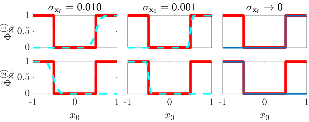
Figure 4: For a one-step time horizon for a Gaussian system with Dirac measure target and avoid sets and an affine control, satisfying (11) results in a Gaussian with standard deviation $\sigma_{\mathbf{x}_{0}}\rightarrow 0$ (right, blue solid). For small values of $\sigma_{\mathbf{x}_{0}}$ (left and middle) discrepancies between the Gaussian (cyan dashed) and Dirac measure (red) that captures the target tube probability measure are evident.

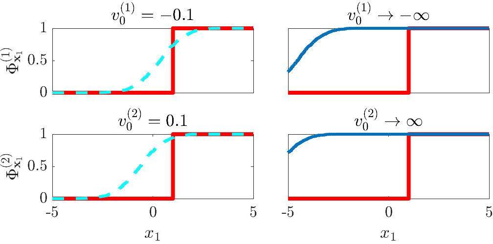
Figure 5: With bounded control authority, for each of the two initial probability measures, $\Phi^{(1)}_{\mathbf{x}_{1}}$ and $\Phi^{(2)}_{\mathbf{x}_{1}}$, it is not possible to construct an affine controller that satisfies (III). This is seen in the fact that the state probability measure $\Phi_{\mathbf{x}_{1}}$ (left, cyan dashed) does not attain the desired value of $1$ before the target probability measure (red) does (as $x_{1}$ increases). In contrast, if we were to allow infinite control authority (right), the feedforward gain of $v_{0}\rightarrow\infty$ (respectively $v_{0}\rightarrow-\infty$) would satisfy (III).

V-B Random Target and Avoid Sets

We now consider target and avoid sets that are random, meaning that the set takes a probabilistic representation. For a Bernoulli random variable $\mathbf{y}$ with $p=0.2$ and $q=0.8$, the target set is $\mathcal{T}$ is random, with the set $\mathcal{T}_{1}$ evaluated with 20% likelihood or $\mathcal{T}_{2}$ evaluated with 80% likelihood, where $\mathcal{T}_{1}=\{x\in\mathbb{R}:x\leq-0.5\}$ and $\mathcal{T}_{2}=\{x\in\mathbb{R}:x\leq-1\}$. The resulting target probability measure is $\mu_{\mathcal{T}}(x)=0.2\cdot\delta_{x}(\mathcal{T}_{1})+0.8\cdot\delta_{x}(\mathcal{T}_{2})$. For the target tube probability measure, consider the same $\mathbf{y}$ such that $\mu_{\mathcal{A}^{\complement}}(x)=0.2\cdot\delta_{x}(\mathcal{A}_{1}^{\complement})+0.8\cdot\delta_{x}(\mathcal{A}_{2}^{\complement})$, for $\mathcal{A}_{1}^{\complement}=\{x\in\mathbb{R}:\ x\leq-0.5\ \mathrm{or}\ x\geq 0.5\}$ and $\mathcal{A}_{2}^{\complement}=\{x\in\mathbb{R}:\ x\leq-1\ \mathrm{or}\ x\geq 1\}$.

This case follows a similar argument to the non-random sets, in which $\Phi_{\mathbf{x}_{0}}$ satisfies (11) and $\Phi_{\mathbf{x}_{1}}$ satisfies (III), almost surely. Thus, we have two possible state probability measures in the form of $\Phi_{\mathbf{x}_{0}}(x_{0})=p\cdot\Phi_{\mathbf{x}_{0,1}}(x_{0})+q\cdot\Phi_{\mathbf{x}_{0,2}}(x_{0})$ which is a mixture of Gaussian probability measures where for $p=0.2$ with mean $m_{\mathbf{x}_{0,1}}$ and standard deviation $\sigma_{\mathbf{x}_{0,1}}$ and $q=0.8$ with $m_{\mathbf{x}_{0,2}}$ and $\sigma_{\mathbf{x}_{0,2}}$. We use a similar normal approximation argument as in the non-random case, resulting in $m^{(1)}_{\mathbf{x}_{0,1}}=0.5$, $m^{(1)}_{\mathbf{x}_{0,2}}=1$ and $m^{(2)}_{\mathbf{x}_{0,1}}=-0.5$, $m^{(2)}_{\mathbf{x}_{0,2}}=-1$ with all $\sigma_{\mathbf{x}_{0,1}},\sigma_{\mathbf{x}_{0,2}}\rightarrow 0$, as shown in Figure 6.

Similarly to the previous analysis, it is not possible to satisfy (III) with bounded control authority, as shown in Figure 7 (left column). Satisfaction of (III) would require the standard deviation of the mixture of Gaussian probability measure, $\Phi_{\mathbf{x}_{1}}$, to approach zero, which would require $v_{0}$ to be infinite and $h_{0}=0$ (right column).

As in the non-random set case, we cannot assure (III) due to the affine controller and Gaussian probability measure, as shown in Figure 7 (left) for the value of $v_{k}$ which saturates the control (with $h_{0}=0$). For (III) to be satisfied, we require $v_{0}\rightarrow-\infty$ (right), which, as in the previous case, requires infinite control authority.

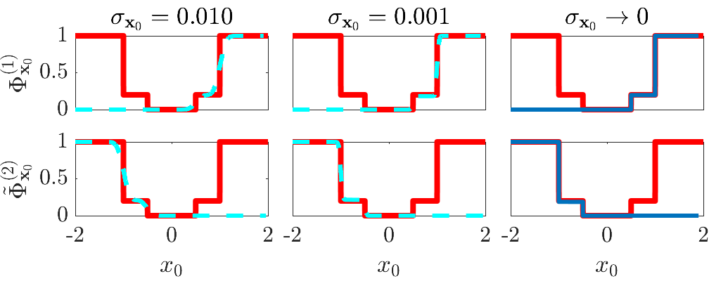
Figure 6: With random target and avoid sets (defined according to a Bernoulli random variable) and an affine control, satisfying (11) results in a mixture of Gaussian probability measures with the same standard deviation $\sigma_{\mathbf{x}_{0}}\rightarrow 0$ (right, blue solid). As in Figure 4, we note that for small, finite values of $\sigma_{\mathbf{x}_{0}}$ (left and middle) discrepancies between the initial state probability measure (cyan, dashed) and the Dirac measure that captures the target tube probability measure (red) are evident.

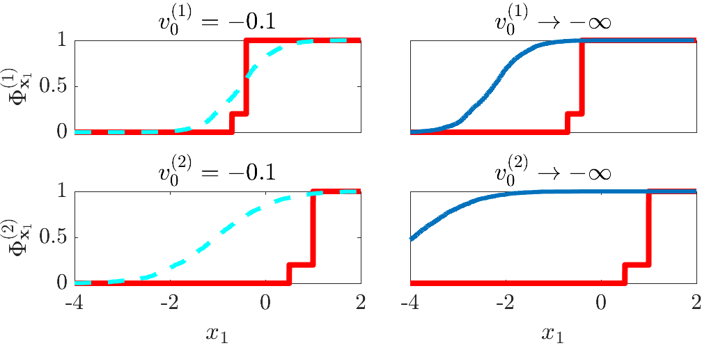
Figure 7: With bounded control authority, it is not possible to construct affine controllers that satisfy (III). Following the same logic as in Figure 5, $\Phi_{\mathbf{x}_{1}}$ (left, cyan dashed) does not attain the value of 1 before the target probability measure (red) as $x_{1}$ increases. However, if infinite control authority was allowed (right), then $v_{0}\rightarrow-\infty$ would satisfy (III).

VI Conclusion

We present a framework for stochastic reachability via probability measures. Given a Markov feedback policy, we establish the existence of the backward recursion of state probability measures. Then, we establish the conditions under which there exists a Markov feedback policy that minimizes a Wasserstein distance, ensuring satisfaction of propagation of the probability measures in a manner that respects reachability specifications. Future work will focus on relationships to the standard stochastic reachability problem and relaxations that exploit computational advantages of the Wasserstein distance.

References

• [1] K. Lesser, M. Oishi, and R. S. Erwin, “Stochastic reachability for control of spacecraft relative motion,” in IEEE Conference on Decision and Control, 2013, pp. 4705–4712.
• [2] A. Abate, H. Blom, N. Cauchi, S. Haesaert, A. Hartmanns, K. Lesser, M. Oishi, V. Sivaramakrishnan, S. Soudjani et al., “ARCH-COMP18 category report: Stochastic modelling.” in 5th International Workshop on Applied Verification of Continuous and Hybrid Systems, vol. 54, 2018, pp. 71–103.
• [3] A. Abate, H. Blom, J. Delicaris, S. Haesaert, A. Hartmanns, B. van Huijgevoort, A. Lavaei, H. Ma, M. Niehage, A. Remke et al., “ARCH-COMP22 category report: Stochastic models,” in Proc. of 9th International Workshop on Applied Verification of Continuous and Hybrid Systems, vol. 90, 2022, pp. 113–141.
• [4] A. Abate, M. Prandini, J. Lygeros, and S. Sastry, “Probabilistic reachability and safety for controlled discrete time stochastic hybrid systems,” Automatica, vol. 44, no. 11, pp. 2724–2734, 2008.
• [5] S. Summers and J. Lygeros, “Verification of discrete time stochastic hybrid systems: A stochastic reach-avoid decision problem,” Automatica, vol. 46, no. 12, pp. 1951–1961, 2010.
• [6] S. Soudjani, C. Gevaerts, and A. Abate, “Faust: Formal Abstractions of Uncountable-STate STochastic processes,” in Tools and Algorithms for the Construction and Analysis of Systems: 21st International Conference, TACAS 2015, London, UK, April 11-18, 2015, Proc. 21.   Springer, 2015, pp. 272–286.
• [7] N. Cauchi and A. Abate, “StocHy-automated verification and synthesis of stochastic processes,” in Proc. 22nd ACM International Conference on Hybrid Systems: Computation and Control, 2019, pp. 258–259.
• [8] H. Sartipizadeh, A. Vinod, B. Açikmeşe, and M. Oishi, “Voronoi partition-based scenario reduction for fast sampling-based stochastic reachability computation of linear systems,” in American Control Conference, 2019, pp. 37–44.
• [9] A. Vinod and M. Oishi, “Stochastic reachability of a target tube: Theory and computation,” Automatica, vol. 125, p. 109458, 2021.
• [10] N. Kariotoglou, S. Summers, T. Summers, M. Kamgarpour, and J. Lygeros, “Approximate dynamic programming for stochastic reachability,” in 2013 European Control Conference, 2013, pp. 584–589.
• [11] A. Halder and E. Wendel, “Finite horizon linear quadratic gaussian density regulator with wasserstein terminal cost,” in American Control Conference, 2016, pp. 7249–7254.
• [12] J. Pilipovsky and P. Tsiotras, “Covariance steering with optimal risk allocation,” IEEE Transactions on Aerospace and Electronic Systems, vol. 57, no. 6, pp. 3719–3733, 2021.
• [13] I. Balci and E. Bakolas, “Exact SDP formulation for discrete-time covariance steering with Wasserstein terminal cost,” arXiv preprint arXiv:2205.10740, 2022.
• [14] V. Sivaramakrishnan, J. Pilipovsky, M. Oishi, and P. Tsiotras, “Distribution steering for discrete-time linear systems with general disturbances using characteristic functions,” in 2022 American Control Conference, 2022, pp. 4183–4190.
• [15] Y. Guan, M. Afshari, and P. Tsiotras, “Zero-sum games between mean-field teams: A common information and reachability based analysis,” arXiv preprint arXiv:2303.12243, 2023.
• [16] A. Devonport, F. Yang, L. El Ghaoui, and M. Arcak, “Data-driven reachability analysis with Christoffel functions,” in 2021 60th IEEE Conference on Decision and Control, 2021, pp. 5067–5072.
• [17] G. Peyré and M. Cuturi, “Computational optimal transport: With applications to data science,” Foundations and Trends in Machine Learning, vol. 11, no. 5-6, pp. 355–607, 2019.
• [18] T. Tao, Analysis 1.   Springer, 2009, vol. 185.
• [19] C. Villani, Optimal transport: Old and new.   Springer, 2009, vol. 338.
• [20] Y. Chow and H. Teicher, Probability Theory: Independence, Interchangeability, Martingales.   Springer New York, 1997.
• [21] V. Bogachev, Measure theory.   Springer Berlin, Heidelberg, 2007.
• [22] D. Bertsekas and S. E. Shreve, Stochastic optimal control: The discrete-time case.   Athena Scientific, 1996.
• [23] S. Summers, M. Kamgarpour, C. Tomlin, and J. Lygeros, “Stochastic system controller synthesis for reachability specifications encoded by random sets,” Automatica, vol. 49, no. 9, pp. 2906–2910, 2013.
• [24] M. Pereyra and L. Ward, Harmonic analysis: From Fourier to wavelets.   American Mathematical Soc., 2012, vol. 63.