The communication complexity of functions with large outputs

Abstract

We study the two-party communication complexity of functions with large outputs, and show that the communication complexity can greatly vary depending on what output model is considered. We study a variety of output models, ranging from the open model, in which an external observer can compute the outcome, to the XOR model, in which the outcome of the protocol should be the bitwise XOR of the players’ local outputs. This model is inspired by XOR games, which are widely studied two-player quantum games.

We focus on the question of error-reduction in these new output models. For functions of output size $k$, applying standard error reduction techniques in the XOR model would introduce an additional cost linear in $k$. We show that no dependency on $k$ is necessary. Similarly, standard randomness removal techniques, incur a multiplicative cost of $2^{k}$ in the XOR model. We show how to reduce this factor to $O(k)$.

In addition, we prove analogous error reduction and randomness removal results in the other models, separate all models from each other, and show that some natural problems – including Set Intersection and Find the First Difference – separate the models when the Hamming weights of their inputs is bounded. Finally, we show how to use the rank lower bound technique for our weak output models.

1 Introduction

Most of the literature on the topic of communication complexity has focused on Boolean functions. The usual definition stipulates that at the end of the protocol, one of the players knows the value of the function. In the rectangle based lower bounds, the assumption is slightly stronger: at the end of the protocol, the transcript of the protocol determines a combinatorial rectangle of inputs that all evaluate to the same outcome. This means that given the transcript (together with the public coins, in the randomized public-coin setting), an external observer can determine the output. In the case of Boolean functions, this assumption makes no significant difference since the player who knows the value of the function can send it in the last message of the protocol, at an additional cost of at most one bit. When the function has large outputs, however, sending the value of the function as part of the transcript could cost more than all the prior communication. When this happens, then what should be considered the “true” communication complexity of the problem?

When studying functions with large outputs, several fundamental questions and issues emerge. What lower bound techniques extend to non-Boolean functions? When composing protocols with large outputs, it may not be useful for both players to know the values of the intermediate functions, and the aggregated cost of relaying the outcome at each intermediate step could exceed the complexity of the composed problem. These issues are also applicable to information complexity, where the cost is measured in information theoretic terms instead of in number of bits of communication. Requiring protocols to reveal the outcome as part of the transcript could be an obstacle to finding very low information protocols. It also raises the following issue: how does one amplify success when outputs are large? Amplification schemes typically involve repeating a protocol and taking a majority outcome, but finding said majority outcome naïvely incurs a cost that depends on the length of the output. We explore these issues, and give new models and amplification schemes.

Well-studied examples of functions with large outputs include asymmetric games, like the NBA problem [Orl90, Orl91] (see also [KN97, Example 4.53, p. 64]), and many problems where the output is essentially of the same size as the input (e.g., computing the intersection of two sets [BCK⁺14, BCK⁺16]). A decisional analog of a function with large output may have a similar communication complexity (e.g., Set Disjointness [KS92, Raz92, BYJKS04]) or a very different one (e.g., deciding if the parties’ numbers sum to something greater than a given constant [Nis93, Vio15]). Large output functions also appear when studying whether multiple instances of the same function exhibit economies of scale, known as direct sum problems, along with their variants such as agreement and elimination [Aar05, ABG⁺01, BDKW14]. In these and other problems, computing one bit of the output can be just as hard or significantly easier than computing the full output, depending on the function and on the model. Finally, simulation protocols, whose output are transcripts of another protocol, have played a key role in compression [BR14, Bra15, Kol16, She18, BK18] as well as structural results [BBK⁺16, GKR16, GKR21, RS18]. The Find the First Difference problem has been instrumental in compression protocols. Better protocols are known when weaker output conditions are required [BBCR13, BMY15].

1.1 Output models

We put forward several natural alternatives to the model where the transcript and public randomness reveal (possibly without containing it explicitly) the value of the function (we call this the open model). In the local model, both players can determine the value of the function locally (but an external observer might not be able to do so – unlike in the open model). In the unilateral model, one player always learns the answer. In the one-out-of-two model, the player who knows the answer can vary. In the split model, the bits of the output are split between the players in an arbitrary way known to both players. Finally, in the XOR model, each player outputs a string and the result is the bitwise XOR of these outputs. The models form a hierarchy, shown in Fig. 1. We defer formal definitions to Appendix A.

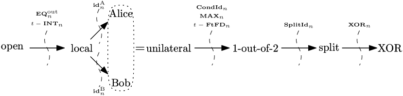
Figure 1: The various models of communication and problems separating them. An arrow from A to B indicates that a communication protocol for a task of type A is also a communication protocol for a task of type B. Details of the separations are provided in Appendices A and H.

In the context of protocols, we make a distinction between what the players output and what the protocol computes. For example, in the XOR model, players output strings $a$ and $b$ but the result of the protocol is $a\oplus b$. We will use the word “output” to designate what the players output at the end of the protocol, and “result” or “outcome” to be the outcome of the protocol (which should be – either probably or certainly – the value or output of the function). Similarly, we will use the term “protocol” to designate the full mechanism for producing the result, and “communication protocol” for the interactive part of the protocol where the players exchange messages, not including the output mechanism.

Among all the models we propose, the XOR model is perhaps the most interesting. This model was partly inspired by (quantum) XOR games, where the players do not exchange any messages (for example [Bel64, PV16, BCMdW10]). One interesting property of the XOR model is that it could be the case, for example, that the output of each player, taken individually, follows a uniform distribution, revealing nothing about either of the inputs or even the value of the function when run as a black box.

Moreover, it is common in communication complexity to consider the complexity of Boolean functions composed with some “gadget” applied to the inputs. For example, for a Boolean function $f$, one can ask what is the communication complexity of $F(u,v)=f(u\oplus v)$, where bitwise XOR is applied as a gadget on the inputs. The XOR model can be seen as applying the XOR gadget to the outputs instead of the inputs: the players output $(a,b)$, and we require $F(u,v)=a\oplus b$ for the computation to be correct.

1.2 Our contributions

We focus on the XOR model where the players each output a string and the outcome of the protocol is the bitwise XOR of these strings.

Error reduction.

We consider the question of error reduction in Section 5. Error reduction is usually a simple task: repeat a computation enough times, and take the majority outcome. However, in the XOR model, neither of the players knows any of the outcomes, so neither can compute the majority outcome without additional communication. Sending over all the outcomes so one of the players can compute the majority would add a prohibitive $\Theta(k)$ term, where $k$ is the length of the output. Removing this dependency on $k$ is possible, however, and doing so requires quite elaborate protocols that highlight the inherent limitations of the XOR model (Theorem 5.3).

We further improve the dependency on the error parameter $\epsilon$ for direct sum problems (Theorem 5.8), by combining protocols for amortized Equality [FKNN95] and Find the First Difference [FRPU94], as well as Gap Hamming Distance [IW03, CR12, Vid12, She12].

Deterministic versus randomized complexity.

In Section 6, we revisit the classical result that states that for any Boolean function, the deterministic communication complexity is at most exponential in the private coin randomized complexity. Once again, if the size of the output is $k$, then applying existing schemes naively to our weaker models adds a multiplicative cost of $2^{k}$. We show that a dependency of a factor of $k$ suffices (Theorem 6.4).

Gap Majority composed with XOR.

To prove our results for the XOR model, we consider the non-Boolean Gap Majority problem composed with an XOR gadget. In the standard majority problem, the input is a set of elements and the goal is to find the element which appears most often. The gap majority problem adds the promise that the majority element should appear at least some a fixed fraction (more than half) of the time. Composition with an XOR gadget turns the problem into a communication complexity problem (see Section 5 and Appendix G). We show that the communication complexity of this problem is closely related to the problems of reducing error and removing randomness in the XOR model.

Other models and separations.

We define several communication models and give problems that maximally separate them (Appendix A). We revisit error reduction and randomness removal in other models (Appendices D and F). The randomness removal scheme for the one-out-of-two model uses a variant of the NBA problem in a subtle way as part of the reconciliation of the majority candidates of the two players. We reduce the dependency on $k$ to a factor of $\log(k)$ in the one-out-of-two model, and remove this dependency entirely when the error parameter $\epsilon$ is bounded by $1/3$ (Theorem F.4).

Finally, we study a few additional problems which exhibit gaps between our various communication models. In particular, several common problems exhibit a gap when the Hamming weights of their inputs are bounded (Appendix H).

Rank lower bound.

We show how lower bound techniques can be adapted to our weak output models by revisiting the notion of monochromatic rectangles associated with the leaves of a protocol tree. We focus on the rank lower bound on deterministic communication and show that it can be used in all of our models, including the XOR model. (Section 7)

It is important to note that our results mostly do not apply to large-output relations (such as the variants of direct sum, elimination and agreement), as many of our proofs crucially rely on the fact that there is a single correct answer.

2 Related work

Previous works have addressed the question of the output model for large output functions. Braverman et al. [BRWY13] make a distinction between “simulation” and “strong simulation” of a protocol. In a strong simulation, an external observer can determine the result without any knowledge of the inputs. In their paper on compression to internal information [BMY15], Bauer et al. stress the importance, when compressing to internal information, that the compression itself need not reveal information to an external observer. They consider two output models which they call internal and external computation. In external computation (which we call the open model), an external observer can determine the result of the protocol, whereas in internal computation (which we call the local model), the players both determine the result at the end of the protocol. They observe that in the deterministic setting, for total functions, the two models coincide, but they can differ in the distributional setting. They consider a key problem of finding the first bit where two strings differ, when each player has one of the two strings. This problem is used in reconciliation protocols to find the first place where transcripts differ. Feige et al. [FRPU94] externally (openly) solve Find the First Difference in $O(\log(\frac{n}{\epsilon}))$, which was shown to be tight by Viola [Vio15]. Bauer et al. [BMY15] give an internal (local) protocol with a better complexity, where the improvement depends on the entropy of the input distribution.

3 Preliminaries

An introduction to communication complexity can be found in Kushilevitz and Nisan’s [KN97], and Rao and Yehudayoff’s [RY20] textbooks.

We denote by $\mathcal{X}$ (resp. $\mathcal{Y}$) the set of inputs of Alice (resp. Bob), $\mathcal{R}_{\mathsf{A}}$ her private randomness ($\mathcal{R}_{\mathsf{B}}$ for Bob), and $\mathcal{R}^{\mathsf{pub}}$ the public randomness accessible to both players. When $\lvert\mathcal{X}\rvert=\lvert\mathcal{Y}\rvert$, we denote by $n$ the size of the input (so that $n=\lceil\log(\lvert\mathcal{X}\rvert)\rceil$). When computing a function, we denote by $k$ the length of the output, $\mathcal{Z}$ the image of the function and $k=\lceil\log(\lvert\mathcal{Z}\rvert)\rceil$. We sometimes consider an additional output symbol $\top$.

We define a full protocol as the combination of a communication protocol and an output mechanism (this is discussed in Appendix A). We define a (two-player) communication protocol $\Pi$ as a full binary tree where each non-leaf node $v$ is assigned a player $\mathcal{P}^{v}$ amongst $A$(lice) and $B$(ob), and a mapping $\mathcal{N}^{v}$ into $\{0,1\}$ whose input space depends on which player the node was assigned to. When $\mathcal{P}^{v}=A$ (resp. $B$) then $\mathcal{N}^{v}$’s input space is $\mathcal{X}\times\mathcal{R}_{\mathsf{A}}\times\mathcal{R}^{\mathsf{pub}}$ (resp. $\mathcal{Y}\times\mathcal{R}_{\mathsf{B}}\times\mathcal{R}^{\mathsf{pub}}$). Note that the tree and each node’s owner are fixed and do not depend on the input. In an execution of a communication protocol, the two players walk down the tree together, starting from the root, until they reach a leaf. Each step down the tree is done by letting the player who owns the current node $v$ apply its corresponding mapping $\mathcal{N}^{v}$, and sending the result to the other player. If it is $0$, the players replace the current node by its left child, and otherwise by its right child. The communication cost ${\operatorname{CC}}(\Pi)$ of a protocol $\Pi$ is the total number of bits exchanged for the worst case inputs.

Since an execution of a communication protocol $\Pi$ is entirely defined by the players’ inputs ($(x,y)\in\mathcal{X}\times\mathcal{Y}$) and the randomness (the players’ private randomness $r_{\mathsf{A}}\in\mathcal{R}_{\mathsf{A}}$ and $r_{\mathsf{B}}\in\mathcal{R}_{\mathsf{B}}$ as well as the public randomness $r\in\mathcal{R}^{\mathsf{pub}}$), we also view the communication protocol as a function $\Pi:\mathcal{X}\times\mathcal{Y}\times\mathcal{R}_{\mathsf{A}}\times\mathcal{R}_{\mathsf{B}}\times\mathcal{R}^{\mathsf{pub}}\rightarrow\{0,1\}^{*}$ whose values we call transcripts of $\Pi$. For the purposes of this paper, we do not include the public randomness as part of the transcript. For a given protocol $\Pi$, we denote by $T_{\pi}=\Pi(X,Y,R_{\mathsf{A}},R_{\mathsf{B}},R)$ the random variable over transcripts of the protocol that naturally arises from $X$, $Y$, $R_{\mathsf{A}}$, $R_{\mathsf{B}}$, and $R$, taken as random variables. We denote by $\mathcal{T}_{\pi}$ the support of the distribution $T_{\pi}$. We denote by $x,y,z,r_{\mathsf{A}},r_{\mathsf{B}},r,t_{\pi}$ elements of the sets $\mathcal{X},\mathcal{Y},\mathcal{Z},\mathcal{R}_{\mathsf{A}},\mathcal{R}_{\mathsf{B}},\mathcal{R}^{\mathsf{pub}},\mathcal{T}_{\pi}$, respectively, which in turn are the supports of the random variables $X,Y,Z,R_{\mathsf{A}},R_{\mathsf{B}},R,T_{\pi}$.

We recall definitions and known bounds of functions that will be used in this paper. For all of these problems, note that the communication complexity is of the same order of magnitude whether we require that both players know the output or only one of them, since the size of the output is no larger than the communication required for one player to know the output. In the remainder of this section, we denote by $R_{\epsilon}(f)$ the minimal communication cost of a randomized protocol computing function $f$ with error at most $\epsilon$ when, say, Bob outputs. $D(f)=R_{0}(f)$ denotes the deterministic communication complexity.

Definition 3.1 (Find the First Difference problem).

$\mathbf{FtFD}_{n}:\{0,1\}^{n}\times\{0,1\}^{n}\rightarrow\{0,\ldots,n\}$ is defined as $\mathbf{FtFD}_{n}(x,y)=\min(\{i:x_{i}\neq y_{i}\}\cup\{n\}).$

Proposition 3.2.

For any $0<\epsilon<\frac{1}{2}$, $R_{\epsilon}(\mathbf{FtFD}_{n})\in\Theta(\log(n)+\log(1/\epsilon))$ [FRPU94, Vio15].

The upper bound uses a walk on a tree where steps are taken according to results from hash functions. The lower bound is from a lower bound on the Greater Than function $\mathbf{GT}_{n}$, which reduces to $\mathbf{FtFD}_{n}$. For a good exposition of the upper bound, see Appendix C in [BBCR13].

Definition 3.3 (Gap Hamming Distance problem).

Let $n,L,U$ be integers such that $0\leq L<U\leq n$. $\mathbf{GHD}_{n}^{L,U}:\{0,1\}^{n}\times\{0,1\}^{n}\rightarrow\{0,1\}$ is a promise problem where the input satisfies the promise that the Hamming distance between inputs $x,y$ is either $\geq U$ or $\leq L$. Then $\mathbf{GHD}_{n}^{L,U}(x,y)=1$ in the first case and $0$ in the second case.

The bounds on Gap Hamming Distance vary depending on the parameters. In this paper we use a linear upper bound which is essentially tight in the regime we require. Many other bounds are known for other regimes [Koz15, CR12, Vid12, She12, BCW98, Wat18].

Definition 3.4 (Equality problem).

The function $\mathbf{EQ}_{n}:\{0,1\}^{n}\times\{0,1\}^{n}\rightarrow\{0,1\}$ is defined as $\mathbf{EQ}_{n}(x,y)={\mathbf{1}}_{x=y}$. The $k$-fold Equality problem is $\mathbf{EQ}_{n}^{\otimes k}((x_{1},\ldots,x_{k}),$ $(y_{1},\ldots,y_{k}))=$ $(\mathbf{EQ}_{n}(x_{1},y_{1}),\ldots,\mathbf{EQ}_{n}(x_{k},y_{k}))$, where $(x_{i},y_{i})\in\{0,1\}^{n}$ for all $i$.

Proposition 3.5.

For $0<\epsilon<\frac{1}{2}$, $R_{\epsilon}(\mathbf{EQ}^{\otimes k}_{n})\in\Theta(k+\log(1/\epsilon))$.

The algorithm from [HPZZ21] which achieves optimal communication uses hashing just like the algorithm for a single instance. It saves on communication compared to $k$ successive uses of a protocol for equality with error $\epsilon/k$ by having players hash all $k$ instances simultaneously, exchange results, and repeat this process, exploiting that they have less and less to communicate about. Intuitively, the number of unequal instances to discover should decrease as the algorithm runs. Once it has been determined for an instance $(x_{i},y_{i})$ that $x_{i}\neq y_{i}$ through unequal hashes, the players do not need to speak further about this instance. An unequal instance is unlikely to survive many tests, which means that late in the algorithm the players can exchange their hashes using that most of them should agree. The idea was also present in previous algorithms [FKNN95] which improved on the trivial algorithm. The lower bound is just from $\Omega(k)$ bits of communication being necessary to send $k$ bits worth of information, even with $\epsilon$ error.

Unless otherwise specified, our protocols use both private and public coins. We use the ‘$\mathsf{priv}$’ superscript when the protocols and mappings do not have access to public randomness.

4 The XOR model

In the XOR model, each player outputs a string and the value of the function is the bitwise XOR of the two outputs (Section 4). This model is inspired by XOR games which have been widely studied in the context of quantum nonlocality as well as unique games.

[XOR computation]definitionxormodel Consider a function $f$ whose output set is $\mathcal{Z}=\{0,1\}^{k}$. A protocol $\Pi$ is said to XOR-compute $f$ with $\epsilon$ error if there exist two mappings $\mathcal{O}_{\mathsf{A}}$ and $\mathcal{O}_{\mathsf{B}}$ with $\mathcal{O}_{\mathsf{A}}:\mathcal{T}_{\pi}\times\mathcal{R}^{\mathsf{pub}}\times\mathcal{R}_{\mathsf{A}}\times\mathcal{X}\rightarrow\{0,1\}^{k}$ and similarly $\mathcal{O}_{\mathsf{B}}:\mathcal{T}_{\pi}\times\mathcal{R}^{\mathsf{pub}}\times\mathcal{R}_{\mathsf{B}}\times\mathcal{Y}\rightarrow\{0,1\}^{k}$ such that for all $(x,y)\in\mathcal{X}\times\mathcal{Y}$,

$$\Pr_{r,r_{\mathsf{A}},r_{\mathsf{B}}}[\mathcal{O}_{\mathsf{A}}(t_{\pi},r,r_{\mathsf{A}},x)\oplus\mathcal{O}_{\mathsf{B}}(t_{\pi},r,r_{\mathsf{B}},y)=f(x,y)]\geq 1-\epsilon.$$

We define $D^{\mathsf{xor}}(f)$ (resp. $R_{\epsilon}^{\mathsf{xor}}(f)$) as the best communication cost of any protocol that computes $f$ in the XOR model with error $\epsilon=0$ (resp. with error at most $\epsilon$, for $0<\epsilon<\frac{1}{2}$). (Notations are defined similarly for our other models with superscripts $\mathsf{open},\mathsf{loc},\mathsf{A},\mathsf{B},\mathsf{uni},\mathsf{spl},\mathsf{1of2}$.)

5 Error reduction and the Gap Majority problem

We study the cost of reducing the error of communication protocols in our weaker models of communication where the outcome of the protocol is not known to both of the players. We focus on the more interesting case of the XOR model in the main text, and results for the other models are in Section D.2.

Standard error reduction schemes work by repeating a protocol many times in order to compute and output the most frequently occurring value among all the executions. Repeating the protocol enough times ensures that with high probability, the output that appears the most is correct. One can derive an upper bound on the number of iterations needed from Hoeffding’s inequality.

Lemma 5.1 (Hoeffding’s inequality).

Let $\left\lparen V_{i}\right\rparen_{i\in[N]}$ be $N$ independent Bernouilli trials of expected value $p$. We have $\Pr\left[\big{\lvert}\tfrac{1}{N}\sum_{i=1}^{N}V_{i}-p\big{\rvert}\geq\delta\right]\leq 2\cdot\exp\left\lparen-\frac{\delta^{2}N}{2p(1-p)}\right\rparen.$

The following holds in the setting where Bob outputs the value of the function at the end of the protocol.

Theorem 5.2.

(Folklore, see [KN97]) Let $0<\epsilon^{\prime}<\epsilon<\frac{1}{2}$, and $C_{\epsilon,\epsilon^{\prime}}=\frac{2\epsilon(1-\epsilon)}{\left\lparen\frac{1}{2}-\epsilon\right\rparen^{2}}\ln\left\lparen\frac{2}{\epsilon^{\prime}}\right\rparen$. For all functions $f:\mathcal{X}\times\mathcal{Y}\rightarrow\mathcal{Z}$, $R^{\mathsf{B}}_{\epsilon^{\prime}}(f)\leq C_{\epsilon,\epsilon^{\prime}}\cdot R^{\mathsf{B}}_{\epsilon}(f).$

Note that it is important here that $f$ is a function, not a relation, so that there is a unique correct output and the player(s) can compute the majority.

In the XOR model, finding the majority result among some number $T$ of runs is much more difficult than in the standard model, since neither of the players can identify reasonable candidates as the majority answer. Exchanging all of the $T$ $k$-bit outputs would result in a bound of $R_{\epsilon^{\prime}}^{\mathsf{xor}}(f)\leq C_{\epsilon,\epsilon^{\prime}}\left\lparen R^{\mathsf{xor}}_{\epsilon}(f)+k\right\rparen.$ We show that this dependence on $k$ is unnecessary.

Theorem 5.3.

Let $0<\epsilon^{\prime}<\epsilon<\frac{1}{2}$, $C_{\epsilon,\epsilon^{\prime}}=8\epsilon{\left\lparen\frac{1}{2}-\epsilon\right\rparen^{-2}}{\ln\left\lparen\frac{8}{\epsilon^{\prime}}\right\rparen}$. For all $f:\mathcal{X}\times\mathcal{Y}\rightarrow\{0,1\}^{k}$, $R^{\mathsf{xor}}_{\epsilon^{\prime}}(f)\leq C_{\epsilon,\epsilon^{\prime}}\cdot R^{\mathsf{xor}}_{\epsilon}(f)+O\left\lparen C_{\epsilon,\epsilon^{\prime}}\right\rparen\ .$

In order to prove this result, we introduce the Gap Majority ($\mathbf{GapMAJ}$) problem, show how Theorem 5.3 reduces to solving $\mathbf{GapMAJ}{\circ}\mathbf{XOR}$ (Lemma 5.5), then give an upper bound on solving $\mathbf{GapMAJ}{\circ}\mathbf{XOR}$ (Theorem 5.6).

The partial function $\mathbf{GapMAJ}_{N,k,\epsilon,\mu}$ has $N$ strings of length $k$ as input and the promise is that there is a string $z$ of length $k$ that appears with $\mu$ weight at least $(1-\epsilon)$ among the $N$ strings, where $\mu$ is a distribution over indices in $[N]$.

Definition 5.4 (Gap Majority).

In the Gap Majority problem $\mathbf{GapMAJ}_{N,k,\epsilon,\mu}:\left\lparen\{0,1\}^{k}\right\rparen^{N}\rightarrow\{0,1\}^{k}$ the input is $(Z_{1},\ldots,Z_{N})$, and $\mu$ is a fixed distribution over the indices $[N]$. When unspecified, $\mu$ is understood to be the uniform distribution. The promise is that $\exists z\in\{0,1\}^{k}$ such that $\mu\left\lparen\left\{i\in[N]:Z_{i}=z\right\}\right\rparen\geq(1-\epsilon)$. Then

$$\mathbf{GapMAJ}_{N,k,\epsilon,\mu}((Z_{i})_{i\in[N]})=z\quad\textrm{s.t.}\quad\mu\left\lparen\left\{i:Z_{i}=z\right\}\right\rparen\geq(1-\epsilon).$$

In $\mathbf{GapMAJ}{\circ}\mathbf{XOR}$, the players are given $N$ strings of length $k$ and their goal is to compute $\mathbf{GapMAJ}$ on the bitwise XOR of their inputs whenever the $\mathbf{GapMAJ}$ promise is satisfied. (Notice that when $k=1$, this is equivalent to the Gap Hamming Distance problem (Definition 3.3) with parameters $L=\epsilon N$, $U=(1-\epsilon)N$.)

For inputs $(X_{1},\ldots,X_{N}),(Y_{1},\ldots,Y_{N})$ to $\mathbf{GapMAJ}_{N,k,\epsilon,\mu}{\circ}\mathbf{XOR}$, we will refer to a pair $(X_{i},Y_{i})$ as a row, and we call $X_{i}$ Alice’s $i$th row, and $Y_{i}$ Bob’s $i$th row. As a warm-up exercise, we show that error reduction reduces to solving an instance of $\mathbf{GapMAJ}{\circ}\mathbf{XOR}$.

Lemma 5.5.

Let $0<\epsilon^{\prime}<\epsilon<\frac{1}{2}$ and $C_{\epsilon,\epsilon^{\prime}}=2\epsilon{\left\lparen\frac{1}{2}-\epsilon\right\rparen^{-2}}{\ln\left\lparen\frac{4}{\epsilon^{\prime}}\right\rparen}$. For every $f:\mathcal{X}\times\mathcal{Y}\rightarrow\{0,1\}^{k}$, $R_{\epsilon^{\prime}}^{\mathsf{xor}}(f)\leq C_{\epsilon,\epsilon^{\prime}}\cdot R_{\epsilon}^{\mathsf{xor}}(f)+R_{\epsilon^{\prime}/2}^{\mathsf{xor}}\left\lparen\mathbf{GapMAJ}_{C_{\epsilon,\epsilon^{\prime}},k,\frac{1}{4}+\frac{\epsilon}{2}}{\circ}\mathbf{XOR}\right\rparen.$

Proof of Lemma 5.5.

Let $\pi$ be a protocol which XOR-computes $f(x,y)$ with $\epsilon$-error and $\pi^{\prime}$ be a protocol which computes $\mathbf{GapMAJ}_{C_{\epsilon,\epsilon^{\prime}},k,\frac{1}{4}+\frac{\epsilon}{2}}{\circ}\mathbf{XOR}$ in the XOR model, with error $\epsilon^{\prime}/2$. We consider the following protocol, which we denote by $\hat{\pi}$: first, run $\pi$ $C_{\epsilon,\epsilon^{\prime}}$ times; then, use the outputs produced by this computation as inputs for $\pi^{\prime}$, run the latter protocol, and output the result. We analyze the new protocol $\hat{\pi}$ as follows. The outputs produced in the first step are strings $X_{1},\cdots,X_{C_{\epsilon,\epsilon^{\prime}}}$ on Alice’s side, and $Y_{1},\cdots,Y_{C_{\epsilon,\epsilon^{\prime}}}$ for Bob. A run of $\pi$ is correct iff $X_{i}\oplus Y_{i}=f(x,y)$. By Hoeffding’s bound (Lemma 5.1), applied with $N=C_{\epsilon,\epsilon^{\prime}}$, $V_{i}=1$ if $X_{i}\oplus Y_{i}\neq f(x,y)$ and $V_{i}=0$ otherwise for $i=1,\dots,N$, $p=\operatorname{\mathbb{E}}[V_{i}]\leq\epsilon$, and $\delta=\frac{1}{2}(\frac{1}{2}-\epsilon)$, we get that with probability at least $1-2e^{-\delta^{2}N/(2p(1-p))}\geq 1-\epsilon^{\prime}/2$, a fraction $p+\delta\leq(\frac{1}{2}+\epsilon)/2$ of the $N$ computations err. In other words, with probability at most $\epsilon^{\prime}/2$, the above strings fail to satisfy the promise in the definition of $\mathbf{GapMAJ}_{C_{\epsilon,\epsilon^{\prime}},k,\frac{1}{4}+\frac{\epsilon}{2}}{\circ}\mathbf{XOR}$. Conditioned on this not happening (i.e., on the promise being met), $\pi^{\prime}$ (hence $\hat{\pi}$) errs with probability at most $\epsilon^{\prime}/2$. The overall error is at most $\epsilon^{\prime}$. ∎

To derive a general upper bound on error reduction using Lemma 5.5, it would suffice to have an upper bound on $R^{\mathsf{xor}}_{\epsilon^{\prime}}(\mathbf{GapMAJ}_{N,k,\epsilon}{\circ}\mathbf{XOR})$. When the error parameter is large ($\epsilon\leq\epsilon^{\prime}$), $\mathbf{GapMAJ}{\circ}\mathbf{XOR}$ in the XOR model is trivial: the players just need to sample a common row and output according to that row. However, Lemma 5.5 requires solving a $\mathbf{GapMAJ}{\circ}\mathbf{XOR}$ instance with small error $\epsilon^{\prime}/2$, which takes us back to square one: finding an error reduction scheme that we can apply to $\mathbf{GapMAJ}{\circ}\mathbf{XOR}$.

In the remainder of the section, we give a protocol for $\mathbf{GapMAJ}{\circ}\mathbf{XOR}$ (Section 5.1) followed by an error reduction scheme for direct sum functions (Section 5.2). In both cases, we use the structure of the XOR function and a protocol for Equality on pairs of rows to find a majority outcome. The error reduction scheme for direct sum functions is a refinement of Lemma 5.5 and is useful in cases where the starting error is very close to $\frac{1}{2}$ and where computing one bit of the output is significantly less costly than computing the full output.

5.1 Solving $\mathbf{GapMAJ}{\circ}\mathbf{XOR}$

Given an instance of $\mathbf{GapMAJ}_{N,k,\epsilon}{\circ}\mathbf{XOR}$, if Alice and Bob pick a row and output what they have on this row, they get the correct output with probability $\geq 1-\epsilon$. Recall that we would like to achieve error $\epsilon^{\prime}<\epsilon$ without incurring a dependence on parameter $k$, which in our application to error reduction corresponds to the length of the output. We show that this is possible.

Theorem 5.6.

Let $0<\epsilon^{\prime}<\epsilon<\frac{1}{2}$, $R^{\mathsf{xor}}_{\epsilon^{\prime}}(\mathbf{GapMAJ}_{N,k,\epsilon}{\circ}\mathbf{XOR})\leq O\left\lparen N+\log\left\lparen\tfrac{1}{\epsilon^{\prime}}\right\rparen\right\rparen\ .$

Proof idea. We use the fact that $a\oplus b=a^{\prime}\oplus b^{\prime}$ iff $a\oplus a^{\prime}=b\oplus b^{\prime}$. Therefore, the players can identify rows that XOR to a same string by solving instances of Equality. This idea alone is enough to obtain a protocol for $\mathbf{GapMAJ}_{N,k,\epsilon}{\circ}\mathbf{XOR}$ of complexity $O\left\lparen N^{2}+\log\left\lparen\tfrac{1}{\epsilon^{\prime}}\right\rparen\right\rparen$ by computing Equality for all $\binom{N}{2}$ pairs of rows to identify the majority outcome. We improve on this by reducing the number of computed Equality instances using Erdős-Rényi random graphs (Lemma 5.7).

Lemma 5.7 (Variation of eq. $(9.18)$ in [ER60]).

Let $G(n,p(n))$ be the distribution over graphs of $n$ vertices where each edge is sampled with independent probability $p(n)$. Let $L_{1}(G)$ be the size of the largest connected component of $G$. Then:

$$\forall\alpha\in[0,1],c\in{\mathbb{R}}^{+},\qquad\Pr\left[L_{1}(G(n,c/n))<(1-\alpha)n\right]\leq e^{\left\lparen\ln(2)-\frac{\alpha}{2}\left\lparen 1-\frac{\alpha}{2}\right\rparen c\right\rparen n}.$$

In particular this probability goes to $0$ as $n$ goes to infinity when $\alpha c>4\ln(2)$.

For completeness, the proof is given in Appendix D.

Proof of Theorem 5.6.

Consider the $\mathbf{GapMAJ}{\circ}\mathbf{XOR}$ instance as a $N\times k$ matrix such that $(X_{i})_{i\in[N]}$ are the rows of Alice and $(Y_{i})_{i\in[N]}$ are the rows of Bob. By the promise of the $\mathbf{GapMAJ}{\circ}\mathbf{XOR}$ problem, we know there exists a $z\in\{0,1\}^{k}$ such that $\{i:X_{i}\oplus Y_{i}=z\}\geq(1-\epsilon)N$. The goal is now for Alice and Bob to identify a row belonging to this large set of rows that XOR to the same $k$-bit string.

Let $i$ and $j$ be the indices of two rows. The event that the two rows XOR to the same string is expressed as $X_{i}\oplus Y_{i}=X_{j}\oplus Y_{j}$, which is equivalent to $X_{i}\oplus X_{j}=Y_{i}\oplus Y_{j}$. This means that we can test whether any two rows XOR to the same bit string with a protocol for Equality.

The protocol goes through the following steps:

1. The players pick rows randomly, enough rows so that with high probability, a constant fraction of the rows XOR to the majority element $z$.

2. The players solve instances of Equality to find large sets of rows that XOR to the same string. In each such large set of rows, they pick a single row. This leaves them with a constant number of candidate rows that might XOR to the majority element $z$.

3. The players decide between those candidates by comparing them with all the rows. There is one candidate row that XORs to the same string as most rows; this row XORs to the majority element $z$.

Step 1.

Using public randomness, Alice and Bob now pick a multiset $S$ of all their rows of size $\lvert S\rvert=T_{\epsilon^{\prime}}=50\ln\left\lparen\frac{10}{\epsilon^{\prime}}\right\rparen$. Each element of $S$ is picked uniformly and independently. Using Hoeffding’s inequality (Lemma 5.1), with probability $\geq 1-\frac{\epsilon^{\prime}}{5}$ more than $\frac{2}{5}$ of those executions XOR to the majority element $z$.

Step 2.

We now consider $S$ as the vertices $V$ of a random graph $G=G(V,E)$, in which each edge is picked with a probability $\frac{c}{\lvert V\rvert}$ with $c>0$. Consider the subgraph $G^{\prime}$ of $G$ induced on the vertices $V^{\prime}\subseteq V$ that correspond to executions that XOR to the majority element $z$. From the previous step, we know that $\lvert V^{\prime}\rvert\geq\frac{2}{5}T_{\epsilon^{\prime}}=20\ln\left\lparen\frac{10}{\epsilon^{\prime}}\right\rparen$. The subgraph $G^{\prime}$ is a random graph where each edge was picked with the same probability $\frac{c}{\lvert V\rvert}=\frac{c^{\prime}}{\lvert V^{\prime}\rvert}$ where $c^{\prime}=c\frac{\lvert V^{\prime}\rvert}{\lvert V\rvert}\geq\frac{2}{5}c$. By Lemma 5.7, this subgraph $G^{\prime}$ contains a connected component of size $\geq(1-\frac{1}{12})\lvert V^{\prime}\rvert\geq\frac{11}{30}\lvert V\rvert$ with probability $\geq 1-2^{-\lvert V^{\prime}\rvert}\geq 1-\frac{\epsilon^{\prime}}{5}$ for $c\geq\frac{720}{143}\ln(2)\approx 3.49$ as $\lvert V^{\prime}\rvert\geq 20\ln\left\lparen\frac{10}{\epsilon^{\prime}}\right\rparen\geq\log{\left\lparen\frac{5}{\epsilon^{\prime}}\right\rparen}$.

At this point, Alice (resp. Bob) computes the bitwise XOR of all pairs of executions that correspond to an edge in $G$: $(X_{i}\oplus X_{j})_{(i,j)\in E,i<j}$ (resp. $(Y_{i}\oplus Y_{j})_{(i,j)\in E,i<j}$). For $\epsilon^{\prime}$ small enough, with high probability ($\geq 1-\frac{\epsilon^{\prime}}{5}$), the set of edges of $G$ is smaller than $2c\cdot T_{\epsilon^{\prime}}$ by Hoeffding’s inequality (the players can abort the protocol otherwise). Then, Alice and Bob solve $\leq 2c\cdot T_{\epsilon^{\prime}}$ instances of Equality with (total) error $\leq\frac{\epsilon^{\prime}}{5}$ to discover a large set of rows that XOR to a same bit string. We now have groups of rows that we know XOR to the same bit string, at least one of which represents more than $\frac{11}{30}$ of $S$’s rows because of the Hoeffding argument combined with the random graph lemma.

Now for each submultiset of rows of $S$ that XOR to the same bit string and represents more than $\frac{11}{30}$ of all of $S$’s rows, pick an arbitrary row in the submultiset. If there is only one such submultiset, Alice and Bob can end the protocol here, outputing the content of the row selected in this submultiset. If there were two such submultisets, then let $i_{1}$ and $i_{2}$ be the indices picked in each submultiset.

Step 3.

To decide between their two candidates, Alice and Bob solve $N$ Equality instances between $X_{i_{1}}{\oplus}X_{j}$ and $Y_{i_{1}}{\oplus}Y_{j}$ for all $j\in[N]$ with error $\leq\frac{\epsilon^{\prime}}{5}$. If more than half of the $N$ rows XOR to the same string as the $i_{1}^{th}$ row, Alice and Bob output their $i_{1}^{th}$ row. Otherwise, they output the other candidate row $i_{2}$.

The complexity of computing $\mathbf{GapMAJ}_{N,k,\epsilon}{\circ}\mathbf{XOR}$ with error $\epsilon^{\prime}<\epsilon$ satisfies

$$R^{\mathsf{xor}}_{\epsilon^{\prime}}\left\lparen\mathbf{GapMAJ}_{N,k,\epsilon}{\circ}\mathbf{XOR}\right\rparen \leq R_{\epsilon^{\prime}/5}\left\lparen\mathbf{EQ}_{k}^{\otimes 2cT_{\epsilon^{\prime}}}\right\rparen+R_{\epsilon^{\prime}/5}\left\lparen\mathbf{EQ}_{k}^{N}\right\rparen\ .$$

To conclude, we apply an amortized protocol for Equality (Proposition 3.5). ∎

Combining Lemma 5.5 and Theorem 5.6 concludes the proof of Theorem 5.3. We will return to the $\mathbf{GapMAJ}{\circ}\mathbf{XOR}$ problem in Appendix G where we give upper bounds in various models (Corollary G.2).

5.2 XOR Error reduction for direct sum functions

The protocol of Theorem 5.3 first generates a full instance of $\mathbf{GapMAJ}{\circ}\mathbf{XOR}$, then solves this instance. The generation of this instance might create an implicit dependency on the output length $k$ of $f$, which in the regime where $\epsilon$ is very close to $1/2$ can be prohibitive. We give a different protocol in which the players are not required to fully generate these intermediate results.

For large output functions, generating one bit of the output can be much less costly than generating all $k$, for example, when $f$ is a direct sum of $k$ instances of a function $g$. We state our stronger amplification theorem for the case of direct sum problems of Boolean functions, but we note that the protocol could be used for other problems where computing one bit of the output is less costly than computing the entire output.

Theorem 5.8.

Let $0<\epsilon^{\prime}<\epsilon<\frac{1}{2}$ and $C_{\epsilon,\epsilon^{\prime}}=8\epsilon{\left\lparen\frac{1}{2}-\epsilon\right\rparen^{-2}}{\ln\left\lparen\frac{12}{\epsilon^{\prime}}\right\rparen}.$ For any $g:\mathcal{X}\times\mathcal{Y}\rightarrow\{0,1\}$ and $f=g^{\otimes k}$,

$$R^{\mathsf{xor}}_{\epsilon^{\prime}}(f) \leq 50\ln\left\lparen\tfrac{12}{\epsilon^{\prime}}\right\rparen\cdot R^{\mathsf{xor}}_{\epsilon}(f)+C_{\epsilon,\epsilon^{\prime}}\cdot R^{\mathsf{xor}}_{\epsilon}(g)+O\left\lparen C_{\epsilon,\epsilon^{\prime}}+\log(k)\right\rparen\ .$$

Notice that the $C_{\epsilon,\epsilon^{\prime}}$ factor – which scales with $\left\lparen\frac{1}{2}-\epsilon\right\rparen^{-1}$ – applies to the complexity of $g$, not of $f$.

Proof idea. Instead of iterating the basic protocol $C_{\epsilon,\epsilon^{\prime}}$ times, we will start by iterating it a smaller number of times which does not depend on $\epsilon$, but only on $\log(\frac{1}{\epsilon^{\prime}})$. This number of iterations suffices to guarantee that the most frequent outcome represents more than a $1/3$ fraction of the rows. If no other outcome represents a large fraction of the rows, we output according to a row from this large fraction. Otherwise, still, at most two outcomes can represent more than a $1/3$ fraction of the rows. We identify a “critical index” of the output function, one that will help us identify the majority result among the two candidate outcomes. We do so by solving a Gap Hamming Distance instance on the critical index. In these remaining $C_{\epsilon,\epsilon^{\prime}}$ runs, we only need one of the $k$ bits of the output.

Details of the proof are given in Appendix E.

6 Deterministic versus randomized complexity

We now turn to removing randomness from private coin protocols.

The standard scheme to derive a deterministic protocol from a private coin protocol proceeds as follows [KN97, Lemma 3.8, page 31]. The players exchange messages to estimate the probability of each transcript. They use the fact that the probability of a transcript can be factored into two parts, each of which can be computed by one of the two players. One of the players sends all of its factors to the other, up to some precision, and the second player can then estimate the probability of each transcript. Each transcript determines an output, therefore from the estimate for the transcripts’ probabilities, this player can derive an estimate for the probability of each output, and output the majority answer.

Theorem 6.1 (Lemma 3.8 in [KN97], page 31).

For any function $f:\mathcal{X}\times\mathcal{Y}\to\mathcal{Z}$ and $0<\epsilon<\frac{1}{2}$, let $R=R^{\mathsf{priv}}_{\epsilon}(f)$. Then $D(f)\leq 2^{R}\left\lparen R+\log\left\lparen\tfrac{1}{\frac{1}{2}-\epsilon}\right\rparen+1\right\rparen.$

Using this well-known result for our output models (first adding $k$ bits of communication to the original protocol of cost $R$ to obtain a protocol that works in the unilateral model) would add $2^{R}R\cdot 2^{k}$ bits to the complexity. For the XOR model, we reduce the dependency to a $O(2^{R}k)$ term. In Appendix F, we show some lower dependencies on $k$ in our other models.

We formalize the problem which we call Transcript Distribution Estimation. Let $\Delta(\mu,\nu)=\frac{1}{2}\sum_{u\in\mathcal{U}}\lvert\mu(u)-\nu(u)\rvert$ be the total variation distance between two probability distributions $\mu$ and $\nu$ over a universe $\mathcal{U}$. For a protocol $\Pi$, let $\mathcal{T}_{\pi}$ be the set of transcripts of $\Pi$, and for $(x,y)\in\mathcal{X}\times\mathcal{Y}$, let us denote by $T^{x,y}_{\pi}$ the distribution over $\mathcal{T}_{\pi}$ witnessed when running $\Pi$ on $(x,y)$.

The key step of the proof of Theorem 6.1 is a protocol (in the standard model) for the following problem.

Definition 6.2 (Transcript Distribution Estimation problem).

For any protocol $\Pi$ and $\delta<\frac{1}{2}$, we say that a protocol $\widetilde{\Pi}$ solves $\mathbf{TDE}_{\Pi,\delta}$ in model $\mathcal{M}$ if, for each input $(x,y)$, $\widetilde{\Pi}$ computes in the sense of model $\mathcal{M}$ a distribution $\widetilde{T}^{x,y}_{\pi}$ such that $\Delta(\widetilde{T}^{x,y}_{\pi},T^{x,y}_{\pi})\leq\delta$.

Lemma 6.3 (Implicit in [KN97], page 31).

Let $\Pi$ be a private coin communication protocol and $\mathcal{T}_{\pi}$ its set of possible transcripts. For any $0<\delta<\frac{1}{2}$, $D(\mathbf{TDE}_{\Pi,\delta})\leq\lvert\mathcal{T}_{\pi}\rvert\cdot\left\lceil\log\left\lparen\frac{\lvert\mathcal{T}_{\pi}\rvert}{\delta}\right\rparen\right\rceil.$

In their proof, Kushilevitz and Nisan [KN97] require only one of the players to learn an estimate of the probability of each leaf. Here we require both players to learn the same estimate, which can be achieved with a factor of two in the communication. Details are given in Lemma F.1 in Section F.1.

In the XOR model, however, sharing such an estimate is not sufficient to remove randomness. At each leaf, each player outputs values with some probability (depending on their private randomness), so there can be as many as $\lvert\mathcal{Z}\rvert$ outputs per leaf by each player, making identifying the majority outcome impossible. We prove the following bound on deterministic communication in the XOR model.

Theorem 6.4.

Let $0<\epsilon<1/2$ and $f:\mathcal{X}\times\mathcal{Y}\rightarrow\mathcal{Z}=\{0,1\}^{k}$. Let $R=R^{\mathsf{xor},\mathsf{priv}}_{\epsilon}(f)$, $M=16\cdot\left\lparen\frac{1}{2}-\epsilon\right\rparen^{-2}\cdot 2^{R}$, and $\epsilon^{\prime}=\frac{5}{8}-\frac{\epsilon}{4}$. Then

$$D^{\mathsf{xor}}(f) \leq D(\mathbf{TDE}_{\Pi_{f},\epsilon^{\prime}-\frac{1}{2}})+D^{\mathsf{xor}}(\mathbf{GapMAJ}_{M,k,\epsilon^{\prime},\mu}{\circ}\mathbf{XOR})$$

$$\leq\left\lparen 2^{R+1}\right\rparen\cdot\left\lparen R+\log\left\lparen\tfrac{8}{\frac{1}{2}-\epsilon}\right\rparen+1\right\rparen+k\cdot\left\lparen\frac{5-2\epsilon}{4}M+1\right\rparen.$$

Where $\mu$ is an unspecified distribution over $[M]$.

Proof idea. We reduce the problem of finding the majority outcome to a much smaller instance of $\mathbf{GapMAJ}{\circ}\mathbf{XOR}$ by discretizing the probabilities of the outputs. This lets us reduce the dependence on the size of the output to just a factor of $k=\log(\lvert\mathcal{Z}\rvert)$ (instead of a factor of $2^{2k}=\lvert\mathcal{Z}\rvert^{2}$).

Proof of Theorem 6.4.

Let $\Pi$ be an optimal private coin XOR protocol for $f$. The players start running the $\mathbf{TDE}_{\Pi,\delta}$ protocol of Lemma F.1 (Lemma 6.3 adapted to the local model, see Section F.1 for details) with $\delta=\frac{1}{4}\left\lparen\frac{1}{2}-\epsilon\right\rparen$, thus learning within statistical distance $\delta$ the probability distribution over leaves that results from the protocol.

Let $o_{\mathsf{A}}(.\mid w,x)$ and $o_{\mathsf{B}}(.\mid w,y)$ be the two independent probability distributions over $\{0,1\}^{k}$ according to which Alice and Bob output, conditioned on reaching leaf $w$, having received inputs $x$ and $y$. To reduce the problem to $\mathbf{GapMAJ}{\circ}\mathbf{XOR}$, they discretize $o_{\mathsf{A}}$ and $o_{\mathsf{B}}$ into $\lceil\delta^{-1}\rceil$ events. Let $\dot{o}_{\mathsf{A}}$ denote the discretization of $o_{\mathsf{A}}$ with following properties for Alice (Similarly for $\dot{o}_{\mathsf{B}}$ for Bob):

$$\forall z,w:\qquad\dot{o}_{\mathsf{A}}(z\mid w,x)\cdot\lceil\delta^{-1}\rceil\in{\mathbb{N}}\quad\text{and}\quad\lvert o_{\mathsf{A}}(z\mid w,x)-\dot{o}_{\mathsf{A}}(z\mid w,x)\rvert\leq\frac{1}{\lceil\delta^{-1}\rceil}.$$

A simple greedy approach to discretization goes like this:

1. Replace all $o_{\mathsf{A}}(z\mid w,x)$ by $\dot{o}_{\mathsf{A}}(z\mid w,x)=\frac{1}{\lceil\delta^{-1}\rceil}\left\lfloor{\lceil\delta^{-1}\rceil}o_{\mathsf{A}}(z\mid w,x)\right\rfloor$.

2. While the probabilities of $\dot{o}_{\mathsf{A}}$ sum to less than $1$, pick a $z$ s.t. $o_{\mathsf{A}}(z\mid w,x)-\dot{o}_{\mathsf{A}}(z\mid w,x)$ is maximal. For that $z$, set $\dot{o}_{\mathsf{A}}(z\mid w,x)=\frac{1}{\lceil\delta^{-1}\rceil}\left\lceil{\lceil\delta^{-1}\rceil}o_{\mathsf{A}}(z\mid w,x)\right\rceil$.

The players then construct a distributional $\mathbf{GapMAJ}{\circ}\mathbf{XOR}$ instance with $M$ rows where $M=\lceil\delta^{-1}\rceil^{2}\lvert\mathcal{T}_{\pi}\rvert$ in the following way:

• For each leaf $w$ the players define $\lceil\delta^{-1}\rceil^{2}$ rows. Rows are indexed by $(i,j)\in\left[\lceil\delta^{-1}\rceil\right]\times\left[\lceil\delta^{-1}\rceil\right]$ and are such that:

  • For each $z$, there are exactly $\left\lceil\delta^{-1}\right\rceil\dot{o}_{\mathsf{A}}(z\mid w,x)$ indices $i_{z}\in\left[\lceil\delta^{-1}\rceil\right]$ such that Alice outputs $z$ on all rows of the form $(i_{z},j),\forall j$.

  • For each $z$, there are exactly $\lceil\delta^{-1}\rceil\dot{o}_{\mathsf{B}}(z\mid w,y)$ indices $j_{z}\in\left[\lceil\delta^{-1}\rceil\right]$ such that Bob outputs $z$ on all rows of the form $(i,j_{z}),\forall i$.

• The probability of the row $(i,j)$ associated to the leaf $w$ under the distribution $\mu$ is taken to be $p^{\mathsf{lf}}(w\mid x,y)\cdot\lceil\delta^{-1}\rceil^{-2}$, where $p^{\mathsf{lf}}(w\mid x,y)$ is the probability of ending in a leaf $w$ in the original protocol $\Pi$. ($\mu$ is the unspecified distribution over $[M]$ in the statement of Theorem 6.4.)

The players then solve the $\mathbf{GapMAJ}{\circ}\mathbf{XOR}$ instance and output the result. Clearly, the above procedure has the previously claimed communication complexity. It remains to show that the players built a valid $\mathbf{GapMAJ}{\circ}\mathbf{XOR}$ instance whose result is $f(x,y)$, that is, picking a random row according to $\mu$ from this $\mathbf{GapMAJ}{\circ}\mathbf{XOR}$ instance gives outputs $z_{\mathsf{A}}$ and $z_{\mathsf{B}}$ on Alice and Bob’s sides such that $z_{\mathsf{A}}\oplus z_{\mathsf{B}}=f(x,y)$ with probability $>\frac{1}{2}$.

1. In the original protocol $\Pi$, let $p^{\mathsf{out}}(z\mid x,y)$ be the probability of computing $z$ (after the XOR), $p^{\mathsf{out}}(z\mid w,x,y)$ that same probability conditioned on the protocol ending in leaf $w$, and for all $w$ let $o_{\mathsf{A}}(.\mid w,x)$ (resp. $o_{\mathsf{B}}(.\mid w,y)$) be the distribution according to which Alice (resp. Bob) outputs once in leaf $w$. Then $p^{\mathsf{out}}(z\mid x,y)$ can be expressed as:

   $$p^{\mathsf{out}}(z\mid x,y) = \sum_{w}p^{\mathsf{lf}}(w\mid x,y)\cdot p^{\mathsf{out}}(z\mid w,x,y)$$

   $$= \sum_{w}p^{\mathsf{lf}}(w\mid x,y)\cdot\sum_{\mathclap{\begin{subarray}{c}z_{\mathsf{A}},z_{\mathsf{B}}\\ z_{\mathsf{A}}\oplus z_{\mathsf{B}}=z\end{subarray}}}o_{\mathsf{A}}(z_{\mathsf{A}}\mid w,x)\cdot o_{\mathsf{B}}(z_{\mathsf{B}}\mid w,x).$$

   By correctness of the protocol, $p^{\mathsf{out}}(f(x,y)\mid x,y)\geq 1-\epsilon$.

2. Consider $p^{\prime\mathsf{lf}}(.\mid x,y)$, $p^{\prime\mathsf{out}}(.\mid x,y)$, $p^{\prime\mathsf{out}}(.\mid w,x,y)$, $\dot{o}_{\mathsf{A}}(.\mid w,x)$ and $\dot{o}_{\mathsf{B}}(.\mid w,y)$ the approximations of the above quantities encountered when building our instance of $\mathbf{GapMAJ}{\circ}\mathbf{XOR}$. The probability $p^{\prime\mathsf{out}}(z\mid x,y)$ that a random row of our weighted $\mathbf{GapMAJ}{\circ}\mathbf{XOR}$ instance corresponds to a given $z$ is:

   $$p^{\prime\mathsf{out}}(z\mid x,y)=\sum_{w}p^{\prime\mathsf{lf}}(w\mid x,y)\cdot\sum_{\mathclap{\begin{subarray}{c}z_{\mathsf{A}},z_{\mathsf{B}}\\ z_{\mathsf{A}}\oplus z_{\mathsf{B}}=z\end{subarray}}}\dot{o}_{\mathsf{A}}(z_{\mathsf{A}}\mid w,x)\cdot\dot{o}_{\mathsf{B}}(z_{\mathsf{B}}\mid w,x).$$

3. $p^{\prime\mathsf{lf}}(.\mid x,y)$ is $\delta$-close to $p^{\mathsf{lf}}(.\mid x,y)$ in statistical distance. $\dot{o}_{\mathsf{A}}(.\mid w,x)$ is point-wise $\delta$-close to $o_{\mathsf{A}}(.\mid w,x)$ (and similarly for $\dot{o}_{\mathsf{B}}$ and $o_{\mathsf{B}}$).

Consider $o_{\mathsf{A}}\cdot o_{\mathsf{B}}$ the distribution over $z\in\{0,1\}^{k}$ defined by $o_{\mathsf{A}}\cdot o_{\mathsf{B}}(z)=\sum_{z^{\prime}}o_{\mathsf{A}}(z^{\prime}\mid w,x)\cdot o_{\mathsf{B}}(z\oplus z^{\prime}\mid w,y)$. Similarly define $o_{\mathsf{A}}\cdot\dot{o}_{\mathsf{B}}$ and $\dot{o}_{\mathsf{A}}\cdot\dot{o}_{\mathsf{B}}$. Item 3 above implies that $\dot{o}_{\mathsf{A}}\cdot\dot{o}_{\mathsf{B}}$ is point-wise $\delta$-close to $o_{\mathsf{A}}\cdot\dot{o}_{\mathsf{B}}$, which is itself point-wise $\delta$-close to $o_{\mathsf{A}}\cdot o_{\mathsf{B}}$. One can check that $\dot{o}_{\mathsf{A}}\cdot\dot{o}_{\mathsf{B}}$ is point-wise $2\delta$-close to $o_{\mathsf{A}}\cdot o_{\mathsf{B}}$.

Using Lemma F.2 (in the appendix) with $V\sim p^{\mathsf{out}}$, $V^{\prime}\sim p^{\prime\mathsf{out}}$, $U\sim p^{\mathsf{lf}}$, $U^{\prime}\sim p^{\prime\mathsf{lf}}$, $V_{u}\sim o_{\mathsf{A}}\cdot o_{\mathsf{B}}$ and $V^{\prime}_{u}\sim\dot{o}_{\mathsf{A}}\cdot\dot{o}_{\mathsf{B}}$, we get that $p$ and $p^{\prime}$ are point-wise $3\delta$-close. Since $\delta$ was taken to be $\frac{1}{4}\left\lparen\frac{1}{2}-\epsilon\right\rparen$, the probability that the random row of the $\mathbf{GapMAJ}{\circ}\mathbf{XOR}$ instance corresponds to $f(x,y)$ is: $p^{\prime\mathsf{out}}(f(x,y))\geq p^{\mathsf{out}}(f(x,y))-3\delta\geq(1-\epsilon)-\frac{3}{4}\left\lparen\frac{1}{2}-\epsilon\right\rparen=\frac{1}{2}+\frac{1}{4}\left\lparen\frac{1}{2}-\epsilon\right\rparen>\frac{1}{2}.$∎

7 Rank lower bounds for weak output models

Since the output requirements are weaker in our new models, standard lower bound techniques may no longer apply. We adapt the standard rank lower bound to all of our output models (Theorem 7.1). While we do not prove any new lower bound with this result, the main contribution of this section is to show how to adapt an existing lower bound to our new communication complexity models. Our techniques can also be applied to other lower bound techniques in a similar fashion.

Reconsidering monochromatic rectangles

Let $f:\mathcal{X}\times\mathcal{Y}\rightarrow{\mathbb{F}}$ where the value of the function is interpreted as an element of a field ${\mathbb{F}}$. The communication matrix associated with $f$ is the matrix whose rows are indexed by elements of $\mathcal{X}$ and columns by elements of $\mathcal{Y}$ and is defined as $M_{f}=(f(x,y))_{x\in\mathcal{X},y\in\mathcal{Y}}$.

In the open model, since there is a mapping from leaf nodes to outputs, a communication protocol partitions the communication matrix into monochromatic rectangles. This is not the case with the other models of computation. In the unilateral and one-out-of-two models, the rectangles at the leaves are “striped” horizontally or vertically (see Fig. 2 for an illustration), since a player can change her answer depending on her input. In the unilateral models, the direction of the stripes is always the same in all rectangles, while the stripes can have different directions in the one-out-of-two model, depending on which player produces the output. The local model is more subtle: the two players can decide to output different elements of ${\mathbb{F}}$ depending of their local information (their input and randomness). Whenever the two players output something different, the result is incorrect, which gives their rectangles a look similar to permutation matrices.

In the rest of this section we will use the term “leaf rectangle” to designate rectangles corresponding to leaves of the protocol tree.

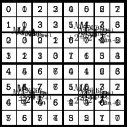
Figure 2: Rectangles corresponding to leaves at the end of a protocol in the open model are monochromatic, while in the unilateral and the one-out-of-two models they have monochromatic “stripes”, by which we mean that they are further partitioned into monochromatic subrectangles by partitioning the rows (for horizontal stripes) or the columns (for vertical stripes) according to what is output by the player responsible for outputting the function value. The direction (horizontal or vertical) depends on which player outputs the value of the function.

The situation of the split and the XOR models is somewhat different, as their leaf rectangles have a more complicated structure. In the XOR model, the leaf rectangles generated by a XOR protocol are similar to the communication matrix for the XOR function $\mathbf{XOR}_{k}$.

Rank lower bound

In order to derive rank lower bounds for our models, we study the ranks of the leaf rectangles. The ranks of the leaf rectangles for the various models imply the following theorem.

Theorem 7.1.

Let $f$ be a total function. Then

$$D^{\mathsf{open}}(f) =D^{\mathsf{loc}}(f)\geq D^{\mathsf{uni}}(f)\geq D^{\mathsf{1of2}}(f)\geq\log\operatorname{rank}(M_{f})$$

$$D^{\mathsf{spl}}(f) \geq\log\operatorname{rank}(M_{f})-1$$

$$D^{\mathsf{xor}}(f) \geq\log\operatorname{rank}(M_{f})-\log(k+1)$$

Proof.

Let us call rank of a rectangle of $M_{f}$ the rank of the submatrix of $M_{f}$ obtained by restricting $M_{f}$ to the rectangle. If there exists a partition of $M_{f}$ into $C$ rectangles such that the rank of each rectangle is bounded by $R$, then $\operatorname{rank}(M_{f})\leq C\times R$. Since for every model $\mathcal{M}$, $M_{f}$ is covered by at most $2^{D^{\mathcal{M}}(f)}$ rectangles of type $\mathcal{M}$, we only need to bound the rank of rectangles of type $\mathcal{M}$ for each model $\mathcal{M}$.

Open, local, unilateral, and one-out-of-two leaf rectangles.

Leaf rectangles of these types are of rank at most $1$, because of their striped structure. Also note that open and local leaf rectangles are similar for total functions in the deterministic setting.

Split leaf rectangles.

Leaf rectangles of this type are of rank at most $2$. Intuitively, this is because the leaf rectangles in this model are of the following form: there exists numbers $a_{1},\ldots,a_{s}$ and $b_{1},\ldots,b_{t}$ such that the value of the cell $(i,j)$ of the rectangle of size $s\times t$, is $a_{i}+b_{j}$. The rectangle is then the product of the following two rank-$2$ matrices: the $s\times 2$ matrix containing the values $a_{1}$ to $a_{s}$ in the first column and the value $1$ in all cells of the second column and the $2\times t$ matrix containing only the value $1$ in its first line and the values $b_{1}$ to $b_{t}$ in the second line, as shown in Fig. 3.

Figure 3: A matrix whose cells $M_{i,j}$ can be expressed as the sum of the $i$th entry of a first vector and the $j$th entry of another one is of rank at most 2. Split rectangles follow this pattern.

More formally: consider how the $k$ bits of the output are split between the two players: let us consider the $k$ bit string $(s_{i})_{1\leq i\leq k}$ such $s_{i}=1$ iff Alice outputs the $i^{th}$ bit of the output.

Let us now define the $1\times 1$ matrix $S_{0}=\begin{bmatrix}0\end{bmatrix}$, and let $H_{c}$ and $V_{c}$ the matrix transformations defined by:

• $H_{c}(A)=\begin{bmatrix}A&A+c\cdot J\end{bmatrix}$

• $V_{c}(A)=\begin{bmatrix}A\\ A+c\cdot J\end{bmatrix}$

Now we define three series of matrices $S_{1}\ldots S_{k}$, $U_{0}\ldots U_{k}$ and $V_{0}\ldots V_{k}$ such that $S_{i}=U_{i}\times V_{i}$ for all $i$, which will prove that $S_{k}$ has rank at most $2$:

• Let $S_{i+1}=\begin{cases}H_{2^{i}}(S_{i})&\textrm{if $s_{i}=0$}\\ V_{2^{i}}(S_{i})&\textrm{if $s_{i}=1$}\end{cases}$.

• Let $U_{0}=\begin{bmatrix}0&1\end{bmatrix}$ and $V_{0}=\begin{bmatrix}1\\ 0\end{bmatrix}$.

• Let $U_{i+1}=\begin{cases}U_{i}&\textrm{if $s_{i}=0$}\\ \begin{bmatrix}U_{i}\\ U_{i}+\begin{bmatrix}2^{i}&0\\ \vdots&\vdots\\ 2^{i}&0\end{bmatrix}\end{bmatrix}&\textrm{if $s_{i}=1$}\end{cases}$

• Let $V_{i+1}=\begin{cases}\begin{bmatrix}V_{i}&V_{i}+\begin{bmatrix}0&\ldots&0\\ 2^{i}&\ldots&2^{i}\end{bmatrix}\end{bmatrix}&\textrm{if $s_{i}=0$}\\ V_{i}&\textrm{if $s_{i}=1$}\\ \end{cases}$

To see that the property $S_{i}=U_{i}\times V_{i}$ is true for all $i\in[k]$, notice that the second column of $U_{i}$ and the top row of $V_{i}$ only contain $1$’s, since this is true for $i=0$ and the property is preserved as $i$ increases. Adding a constant $c$ to the second half of the second line of $V_{i}$, this constant gets multiplied by the second column of $U_{i}$, that only contains $1$’s. The end result is that we add a $c\cdot J$ matrix to half of the matrix, which is exactly what we want.

Finally, notice that $S_{k}$ is a matrix containing all that Alice and Bob can output in the split model given a specific split. A leaf rectangle in the split model is a submatrix of a matrix of this form, where some lines and columns have possibly been permuted or duplicated. Therefore, leaf rectangles in the split model have rank at most $2$.

XOR leaf rectangles

We prove that leaf rectangles produced by XOR protocols have rank at most $(k+1)$.

Consider the communication matrix of the $\mathbf{XOR}_{k}$ function. An XOR leaf rectangle can be obtained as a submatrix of this communication matrix, possibly after permuting or duplicating some rows and columns. Thus, it suffices to show that $M_{\mathbf{XOR}_{k}}$ has rank $k+1$. We do this by directly giving a rank $k+1$ decomposition of $M_{\mathbf{XOR}_{k}}$. Consider the following $2^{k}\times 1$ vectors:

• $v^{k}$ is the all-one vector.

• For $0\leq i<k$, $u^{k,i}$ is such that $u^{k,i}_{j}=(-1)^{1+j_{i}}$ (for $0\leq j<2^{k}$). Such vectors are sometimes called Hadamard vectors.

Let $S_{k}$ be the following $2^{k}\times(k+1)$ matrix:

$$S_{k}=\begin{bmatrix}\sqrt{2^{k-1}-2^{-1}}\cdot v&\ {\sqrt{2^{-1}}}\cdot u^{k,0}&\ldots&{\sqrt{2^{k-2}}}\cdot u^{k,k-1}\end{bmatrix}$$

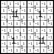
(a)

(b)

(c)

(d)

Figure 4: The $M_{\mathbf{XOR}_{3}}$ communication matrix can be obtained by a linear combination of those matrices.

We have that $S_{k}\prescript{t}{}{S_{k}}=M_{\mathbf{XOR}_{k}}$. Figure 4 gives an intuition of how the $M_{\mathbf{XOR}_{k}}$ matrix is obtained.∎

8 Conclusion and open questions

We have presented output models that are tailored for non-Boolean functions. We hope that these will find many applications, including extensions to information complexity, a better understanding of direct sum problems, simulation protocols, new lower bounds tailored to these models, to name just a few.

The Gap Majority composed with XOR problem (Definition 5.4) is closely related to the Gap Hamming Distance, extended to a large alphabet but with an additional promise, so lower bounds for $\mathbf{GHD}$ do not apply. We conjecture that its deterministic communication complexity is $\Omega(\epsilon Nk)$, matching the trivial upper bound. If true, this would indicate that our randomness removal scheme (Theorem 6.4) is close to tight.

9 Acknowledgments

We thank Jérémie Roland and Sagnik Mukhopadhyay for helpful conversations and the anonymous referees for their numerous suggestions to improve the paper’s presentation. This work was funded in part by the ANR grant FLITTLA ANR-21-CE48-0023.

Appendix A Models for large-output functions

One standard definition of communication complexity requires that at the end of the communication protocol, the output of the computation can be determined from the transcript of the communication and the public randomness (it is the model used in rectangle bounds). It is easy to find examples where such a definition makes it necessary to exchange much more communication than seems natural. For example,

Example A.1.

Consider the function $f:\{0,1\}^{n}\times\{0,1\}^{n}\rightarrow\{0,1\}^{n},f(x,y)=x$, and assume we want to compute it with the promise $x=y$.

A protocol for $f$ requires $n$ bits of communication if the result of the protocol has to be apparent from the communication and the public randomness, even though both players know $f(x,y)$ right from the start.

In this section, we formally define the output models and prove separation results. The most interesting models are arguably the weakest ones: the one-out-of-two (Definition A.9), the split (Definition A.13), and the XOR models (Section 4).

A.1 The open model

We start with the formal definition of our model which reveals the most information regarding the outcome of the computation. We call it the open model.

This is the model for which the partition bounds [JK10], in the form in which they appear in the literature, give lower bounds.

Definition A.2 (Open computation).

A protocol $\Pi$ is said to openly compute $f$ with $\epsilon$ error if there exists a mapping $\mathcal{O}:\mathcal{T}_{\pi}\times\mathcal{R}^{\mathsf{pub}}\rightarrow\mathcal{Z}$ such that: for all $(x,y)\in\mathcal{X}\times\mathcal{Y}$,

$$\Pr_{r,r_{\mathsf{A}},r_{\mathsf{B}}}[\mathcal{O}(t_{\pi},r)=f(x,y)]\geq 1-\epsilon.$$

A.2 The local model

In the previous model, protocols are revealing, in the sense that the result of the computation can not be a secret only known to the players. In the local model, we only require that both players, at the end of the protocol, can output the value of the function (or the same valid output, in the case of a relation).

Definition A.3 (Local computation).

A protocol $\Pi$ is said to locally compute $f$ with $\epsilon$ error if there exist two mappings $\mathcal{O}_{\mathsf{A}}$ and $\mathcal{O}_{\mathsf{B}}$ with $\mathcal{O}_{\mathsf{A}}:\mathcal{T}_{\pi}\times\mathcal{R}^{\mathsf{pub}}\times\mathcal{R}_{\mathsf{A}}\times\mathcal{X}\rightarrow\mathcal{Z}$ and similarly $\mathcal{O}_{\mathsf{B}}:\mathcal{T}_{\pi}\times\mathcal{R}^{\mathsf{pub}}\times\mathcal{R}_{\mathsf{B}}\times\mathcal{Y}\rightarrow\mathcal{Z}$ such that: for all $(x,y)\in\mathcal{X}\times\mathcal{Y}$,

$$\Pr_{r,r_{\mathsf{A}},r_{\mathsf{B}}}[\mathcal{O}_{\mathsf{A}}(t_{\pi},r,r_{\mathsf{A}},x)=\mathcal{O}_{\mathsf{B}}(t_{\pi},r,r_{\mathsf{B}},y)=f(x,y)]\geq 1-\epsilon.$$

Bauer et al. [BMY15] remarked that for total functions and relations, the deterministic open and local communication complexities are the same. Example A.1 shows a separation between the deterministic complexities of computing a function with a promise.

For randomized communication, the local model is separated from the open model by the following total function, as seen in Theorem A.5:

Definition A.4 (Equality with output problem).

$\mathbf{EQ}^{\mathsf{out}}_{n}:\{0,1\}^{n}\times\{0,1\}^{n}\rightarrow\{0,1\}^{n}\cup\{\top\}$ is defined as

$$\mathbf{EQ}^{\mathsf{out}}_{n}(x,y)=\begin{cases}x&\text{if $x=y$}\\ \top&\text{otherwise}\end{cases}$$

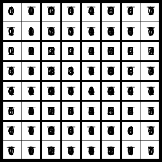
Figure 5: The communication matrix of $\mathbf{EQ}^{\mathsf{out}}_{3}$

Theorem A.5.

$\forall f:\mathcal{X}\times\mathcal{Y}\rightarrow\mathcal{Z}$ with $k=\left\lceil\log\lvert\mathcal{Z}\rvert\right\rceil$ and $\epsilon>0$,

$$R_{\epsilon}^{\mathsf{loc}}(f)\leq R_{\epsilon}^{\mathsf{open}}(f)\leq R_{\epsilon}^{\mathsf{loc}}(f)+k,\quad\text{ and}$$

$$R^{\mathsf{loc}}_{1/4}(\mathbf{EQ}^{\mathsf{out}}_{n})\leq 4,\quad\quad R^{\mathsf{open}}_{1/4}(\mathbf{EQ}^{\mathsf{out}}_{n})\in\Omega(n).$$

We provide a full proof of this theorem, but because all the results of the form $R_{\epsilon}^{\mathcal{M}_{1}}(f)\leq R_{\epsilon}^{\mathcal{M}_{2}}(f)$ or $R_{\epsilon}^{\mathcal{M}_{1}}(f)\leq R_{\epsilon}^{\mathcal{M}_{2}}(f)+k$ for two models $\mathcal{M}_{1}$ and $\mathcal{M}_{2}$ can be proved by essentially the same proof, we will omit them in proofs of later similar theorems, only proving the separation result.

Proof of Theorem A.5.

Proof of $R_{\epsilon}^{\mathsf{loc}}(f)\leq R_{\epsilon}^{\mathsf{open}}(f)$:

An open protocol for a function $f$ is also a local protocol for $f$, as the players can take as mappings $\mathcal{O}_{\mathsf{A}}$ and $\mathcal{O}_{\mathsf{B}}$ the mapping $\mathcal{O}$ of the open protocol (ignoring both players’ randomness and input).

Proof of $R_{\epsilon}^{\mathsf{open}}(f)\leq R_{\epsilon}^{\mathsf{loc}}(f)+k$:

Let $\Pi$ be a local protocol for computing $f$ with error at most $\epsilon$. Consider $\Pi^{\prime}$, the protocol that consists of first running the protocol $\Pi$, and then Alice sends $\mathcal{O}_{\mathsf{A}}(t_{\pi},r,r_{\mathsf{A}},x)$ – what she would output at the end of $\Pi$ to locally compute $f$ – over the communication channel. This only requires $k$ additional bits of communication. Now $\Pi^{\prime}$ is an open protocol, since an external observer can use the last $k$ bits of the transcript as probable $f(x,y)$.

Both the lower bound and the upper bound on $\mathbf{EQ}^{\mathsf{out}}$ directly follow from propositions and theorems previously seen in this manuscript.

Local model upper bound:

The players apply the standard protocol for $\mathbf{EQ}$ (Proposition 3.5). If the strings are different, they output $\top$, otherwise Alice outputs $x$ and Bob outputs $y$.

Open model lower bound:

Consider the mapping $\mathcal{O}$ of the open protocol $\Pi$ and notice that for all $x$, $\Pr_{r}[\mathcal{O}(\Pi(x,x,r),r)=x]\geq 3/4$. Consider that the players have a public randomness source $\mathcal{R}^{\mathsf{pub}}$ that is the uniformly random distribution over $\{0,1\}^{k}$. Then the above statement implies $\lvert\mathcal{O}^{-1}(x)\rvert\geq\frac{3}{4}\cdot 2^{k}$. Since $\cup_{x}\mathcal{O}^{-1}(x)\subseteq\mathcal{T}_{\pi}\times\{0,1\}^{k}$, we have that $\frac{3}{4}\cdot 2^{k}\cdot 2^{n}\leq 2^{{\operatorname{CC}}(\Pi)}\cdot 2^{k}$ hence ${\operatorname{CC}}(\Pi)\geq n+\log\left\lparen\frac{3}{4}\right\rparen\in\Omega(n)$. This is also true when the source of public randomness is not a uniform distribution over $\{0,1\}^{k}$ because of the fact that any non-uniform source of randomness can be simulated with arbitrary precision by a uniform source of randomness.

∎

In Appendix C we generalize this to show that any open protocol for a problem requires $\Omega(k)$ communication. This result follows from a lower bound known as the weak partition bound [FJK⁺16].

A.3 The unilateral models

In this section, we consider models of communication complexity where we require that at the end of the protocol, one player can output the value of the function (or a valid output, in the case of a relation). One-way problems are usually stated in this model.

Definition A.6 (Unilateral computation).

A protocol $\Pi$ is said to Alice-compute $f$ with $\epsilon$ error if there exists a mapping $\mathcal{O}_{\mathsf{A}}:\mathcal{T}_{\pi}\times\mathcal{R}^{\mathsf{pub}}\times\mathcal{R}_{\mathsf{A}}\times\mathcal{X}\rightarrow\mathcal{Z}$ such that: for all $(x,y)\in\mathcal{X}\times\mathcal{Y}$,

$$\Pr_{r,r_{\mathsf{A}},r_{\mathsf{B}}}[\mathcal{O}_{\mathsf{A}}(t_{\pi},r,r_{\mathsf{A}},x)=f(x,y)]\geq 1-\epsilon.$$

Bob-computation is defined in a similar manner.

A protocol is said to unilaterally compute $f$ if it Alice-computes or Bob-computes $f$.

Our definition of the unilateral model corresponds to a minimum of two models, each assigned to a player.

Definition A.7 (Unilateral identity problems).

$\mathbf{id}^{\mathsf{A}}_{n}:\{0,1\}^{n}\times\{0,1\}^{n}\rightarrow\{0,1\}^{n}$ is defined as

$$\mathbf{id}^{\mathsf{A}}_{n}(x,y)=x$$

$id^{\mathsf{B}}_{n}$ is defined similarly, with opposite roles for Alice and Bob.

Figure 6: The communication matrix of $\mathbf{id}^{\mathsf{A}}_{3}$ and $\mathbf{id}^{\mathsf{B}}_{3}$

Theorem A.8.

$\forall f:\mathcal{X}\times\mathcal{Y}\rightarrow\mathcal{Z}$ with $k=\left\lceil\log\lvert\mathcal{Z}\rvert\right\rceil$, $\lambda\in[0,1]$ and $\epsilon>0$

$$R_{\epsilon}^{\mathsf{uni}}(f)\leq R_{\epsilon}^{\mathsf{loc}}(f)\leq R_{\epsilon}^{\mathsf{open}}(f)\leq R_{\epsilon}^{\mathsf{uni}}(f)+k,$$

$$D^{\mathsf{loc}}(f)\leq D^{\mathsf{A}}(f)+D^{\mathsf{B}}(f),\quad\quad R_{\epsilon}^{\mathsf{loc}}(f)\leq R_{\lambda\epsilon}^{\mathsf{A}}(f)+R_{(1-\lambda)\epsilon}^{\mathsf{B}}(f),\quad\text{and}$$

$$D^{\mathsf{uni}}(\mathbf{id}^{\mathsf{A}}_{n})=D^{\mathsf{A}}(\mathbf{id}^{\mathsf{A}}_{n})=D^{\mathsf{B}}(\mathbf{id}^{\mathsf{B}}_{n})=0,\quad\quad R^{\mathsf{loc}}_{1/4}(\mathbf{id}^{\mathsf{A}}_{n})=R^{\mathsf{loc}}_{1/4}(\mathbf{id}^{\mathsf{B}}_{n})\in\Omega(n).$$

The first line also holds for relations, but the second line does not: consider as counterexample the relation $f:\{0,1\}^{n}\times\{0,1\}^{n}\rightarrow 2^{\{0,1\}^{n}},f(x,y)=\{x,y\}$. This problem does not require any communication in both unilateral models ($D^{\mathsf{A}}(f)=D^{\mathsf{B}}(f)=0$), but in the local model, the fact that the players need to agree on a single output makes the communication of order $\Omega(n)$ in both the deterministic and the randomized setting ($D^{\mathsf{loc}}(f)\geq R_{\epsilon}^{\mathsf{loc}}(f)\in\Omega(n)$).

Proof of Theorem A.8.

We omit the proof of the first two lines, that are only based on using the same protocol with the different proper mappings, or sending what one would output in a lower model over the communication channel.

We prove a slightly stronger result for the separation: that $R^{\mathsf{B}}_{1/4}(\mathbf{id}^{\mathsf{A}}_{n})\in\Omega(n)$.

Alice model upper bound:

Alice outputs her $x$, which requires no communication.

Bob model lower bound:

Let us consider $D^{\mathsf{B}}_{1/4}(\mathbf{id}^{\mathsf{A}}_{n},\mu)$ where $\mu$ is the uniform distribution. Bob has to output one of $2^{n}$ equiprobable answers. With communication $C$, Bob can only have $2^{C}$ different answers, so Bob is wrong with probability $\geq 1-2^{C-n}$. Since Bob is supposed to make less than $\frac{1}{4}$ error, we have: $C\geq n+\log\left\lparen\frac{3}{4}\right\rparen$, so $R^{\mathsf{B}}_{1/4}(\mathbf{id}^{\mathsf{A}}_{n})\in\Omega(n)$.

∎

A.4 The one-out-of-two model

In the unilateral models, the player that outputs the result at the end of the protocol is fixed. In particular, it does not depend on the inputs. In the one-out-of-two model, we relax this condition: correctly computing a function in the one-out-of-two model corresponds to an execution such that at the end of the protocol:

• one player outputs a special symbol $\top\not\in\mathcal{Z}$ (which corresponds to silence)

• the other players outputs $f(x,y)$.

Intuitively, we not only require that one of the players outputs the correct answer, but also that she knows that her output is probably correct, while the other knows that other player has a good answer to output. If we were only requiring that one player gives the correct answer, then all Boolean functions would be solved with zero communication in this model. In contrast, our model does not trivialize the communication complexity of Boolean functions.

Definition A.9 (One-out-of-two computation).

A protocol $\Pi$ is said to one-out-of-two compute $f$ with $\epsilon$ error if there exist two mappings $\mathcal{O}_{\mathsf{A}}$ and $\mathcal{O}_{\mathsf{B}}$ with $\mathcal{O}_{\mathsf{A}}:\mathcal{T}_{\pi}\times\mathcal{R}^{\mathsf{pub}}\times\mathcal{R}_{\mathsf{A}}\times\mathcal{X}\rightarrow\mathcal{Z}\cup\{\top\}$ and similarly $\mathcal{O}_{\mathsf{B}}:\mathcal{T}_{\pi}\times\mathcal{R}^{\mathsf{pub}}\times\mathcal{R}_{\mathsf{B}}\times\mathcal{Y}\rightarrow\mathcal{Z}\cup\{\top\}$ such that: for all $(x,y)\in\mathcal{X}\times\mathcal{Y}$,

$$\Pr_{r,r_{\mathsf{A}},r_{\mathsf{B}}}[\left\lparen\mathcal{O}_{\mathsf{A}}(t_{\pi},r,r_{\mathsf{A}},x),\mathcal{O}_{\mathsf{B}}(t_{\pi},r,r_{\mathsf{B}},y)\right\rparen\in\{(f(x,y),\top),(\top,f(x,y))\}]\geq 1-\epsilon.$$

The next proposition shows that any one-out-of-two protocol can be transformed into another one-out-of-two protocol of lesser or equal error and using only one additional bit of communication, such that at the end of the protocol it is always the case that exactly one player outputs a value in $\mathcal{Z}$ and the other stays silent (outputs $\top$).

Proposition A.10.

Consider a function $f:\mathcal{X}\times\mathcal{Y}\rightarrow\mathcal{Z}$ and $\Pi$ a one-out-of-two protocol for $f$ with error $\epsilon>0$ of communication cost $C$. Then there exists a one-out-of-two protocol $\Pi^{\prime}$ of communication cost $(C+1)$ that computes $f$ with the same error but with mappings such that it is always the case that only one of them speaks at the end:

$$\forall x,y,r_{\mathsf{A}},r_{\mathsf{B}},r,t_{\pi^{\prime}}=\Pi^{\prime}(x,y,r_{\mathsf{A}},r_{\mathsf{B}},r):$$

$$\left\lparen\mathcal{O}^{\prime}_{\mathsf{A}}(t_{\pi^{\prime}},r,r_{\mathsf{A}},x),\mathcal{O}^{\prime}_{\mathsf{B}}(t_{\pi^{\prime}},r,r_{\mathsf{B}},y)\right\rparen\in\left\lparen\mathcal{Z}\times\{\top\}\right\rparen\cup\left\lparen\{\top\}\times\mathcal{Z}\right\rparen.$$

Proof of Proposition A.10.

Let $\Pi$ be a one-out-of-two protocol for $f$ and $\mathcal{O}_{\mathsf{A}}$,$\mathcal{O}_{\mathsf{B}}$ the associated mappings. We define the protocol $\Pi^{\prime}$ to be a protocol that first behaves as $\Pi$ (getting a transcript $t_{\pi}$) and when we hit a leaf in the protocol for $\Pi$, Alice sends a bit of communication to Bob following this rule:

• If $\mathcal{O}_{\mathsf{A}}(t_{\pi},r,r_{\mathsf{A}},x)=\top$, Alice sends $0$ to Bob.

• Otherwise Alice sends $1$ to Bob.

Let $c_{\mathsf{A}}$ be this control bit, sent by Alice in the last round of the new protocol $\Pi^{\prime}$. Then, Alice keeps the same mapping $\mathcal{O}_{\mathsf{A}}$ whereas Bob’s new mapping $\mathcal{O}^{\prime}_{\mathsf{B}}$ is such that:

$$\mathcal{O}^{\prime}_{\mathsf{B}}(t_{\pi^{\prime}},r,r_{\mathsf{B}},y)=\begin{cases}\top&\textrm{if $c_{a}=1$},\\ \mathcal{O}_{\mathsf{B}}(t_{\pi},r,r_{\mathsf{B}},y)&\textrm{if $c_{a}=0$ and $\mathcal{O}_{\mathsf{B}}(t_{\pi},r,r_{\mathsf{B}},y)\neq\top$,}\\ z&\textrm{picked u.a.r.\ in $\mathcal{Z}$, otherwise.}\end{cases}$$

Intuitively, Alice tells Bob whether to speak or not, and he obeys. Since the only cases where this changes what the players output is when they were going to both speak or both stay silent, the error does not increase in the process. ∎

Definition A.11 (Conditional identity problem).

The function $\mathbf{CondId}_{n}:\{0,1\}^{n}\times\{0,1\}^{n}\rightarrow\{0,1\}^{n}$ is defined as

$$\mathbf{CondId}_{n}(x,y)=\begin{cases}x&\text{if}\ x_{0}=y_{0},\\ y&\text{otherwise,}\end{cases}$$

where $x_{0}$ is the fist bit of $x$, similarly for $y$.

Figure 7: The communication matrix of $\mathbf{CondId}_{3}$

Theorem A.12.

$\forall f:\mathcal{X}\times\mathcal{Y}\rightarrow\mathcal{Z}$ with $k=\left\lceil\log\lvert\mathcal{Z}\rvert\right\rceil$ and $\epsilon>0$

$$R_{\epsilon}^{\mathsf{1of2}}(f)\leq R_{\epsilon}^{\mathsf{uni}}(f)\leq R_{\epsilon}^{\mathsf{loc}}(f)\leq R_{\epsilon}^{\mathsf{open}}(f)\leq R_{\epsilon}^{\mathsf{1of2}}(f)+k+1,\quad\text{and}$$

$$D^{\mathsf{1of2}}(\mathbf{CondId}_{n})\in O(1),\quad\quad R^{\mathsf{uni}}_{\epsilon}(\mathbf{CondId}_{n})\in\Omega(n).$$

Proof of Theorem A.12.

Again, we focus on the separation result.

One-out-of-two model upper bound:

Alice and Bob send each other $x_{0}$ and $y_{0}$. If $x_{0}=y_{0}$, Alice outputs $x$, otherwise Bob outputs $y$. This only takes $2$ bits of communication.

Unilateral model lower bound:

Let us consider $D^{\mathsf{B}}_{1/4}(\mathbf{CondId}_{n},\mu)$ where $\mu$ is the uniform distribution over $(x,y)$ such that $x_{0}=y_{0}$. Having received any given $x$, Bob has to output one of $2^{n-1}$ equiprobable answers. With communication $C$, Bob can only have $2^{C}$ different answers, so Bob is wrong with probability $\geq 1-2^{C-n+1}$. Since Bob is supposed to make less than $\frac{1}{4}$ error, we have: $C\geq n-1+\log\left\lparen\frac{3}{4}\right\rparen$, so $R^{\mathsf{B}}_{1/4}(\mathbf{CondId}_{n})\in\Omega(n)$. By symmetry, we also have $R^{\mathsf{A}}_{1/4}(\mathbf{CondId}_{n})\in\Omega(n)$, so $R^{\mathsf{uni}}_{1/4}(\mathbf{CondId}_{n})\in\Omega(n)$.

∎

A.5 The split model

In our next model, we allow the answer to be split between the two players. In the one-out-of-two model, one of the player had to output the full output, while the other stayed fully silent. In contrast, in the split model we allow both players to output part of the result. We only require that any given bit is output by exactly one player (the other player stays silent on this particular bit). In a valid split computation, it may be that the first bit of $f(x,y)$ is output by Alice, while the second one is output by Bob.

Definition A.13 (Split computation).

A protocol $\Pi$ is said to split compute $f$ with $\epsilon$ error if there exist two mappings $\mathcal{O}_{\mathsf{A}}$ and $\mathcal{O}_{\mathsf{B}}$ with $\mathcal{O}_{\mathsf{A}}:\mathcal{T}_{\pi}\times\mathcal{R}^{\mathsf{pub}}\times\mathcal{R}_{\mathsf{A}}\times\mathcal{X}\rightarrow\{0,1,*\}$ and similarly $\mathcal{O}_{\mathsf{B}}:\mathcal{T}_{\pi}\times\mathcal{R}^{\mathsf{pub}}\times\mathcal{R}_{\mathsf{B}}\times\mathcal{Y}\rightarrow\{0,1,*\}$ such that: for all $(x,y)\in\mathcal{X}\times\mathcal{Y}$,

$$\Pr_{r,r_{\mathsf{A}},r_{\mathsf{B}}}[\mathcal{O}_{\mathsf{A}}(t_{\pi},r,r_{\mathsf{A}},x)\mathbin{{\mathsf{x\!x}}}\mathcal{O}_{\mathsf{B}}(t_{\pi},r,r_{\mathsf{B}},y)=f(x,y)]\geq 1-\epsilon.$$

where $(a\mathbin{{\mathsf{x\!x}}}b)_{i}\begin{cases}a_{i}&\textrm{if }b_{i}=*,\\ b_{i}&\textrm{if }a_{i}=*,\\ *&\textrm{otherwise}.\end{cases}$

We call weave the binary operator $\mathbin{{\mathsf{x\!x}}}:\{0,1,*\}^{k}\times\{0,1,*\}^{k}\rightarrow\{0,1,*\}^{k}$ described at the end of Definition A.13, that recombines the parts split among the players.

To separate this model from the one-out-of-two model, we introduce a problem where the information about the output is naturally split between the two players. We do so in a manner which makes computing this problem in the split model trivial, while the fact that one of the players must aggregate complete information about the output in the one-out-of-two model leads to a large amount of communication.

Definition A.14 (Split identity problem).

$\mathbf{SplitId}_{n}:\{0,1\}^{n}\times\{0,1\}^{n}\rightarrow\{0,1\}^{n}$ is defined as

$$\mathbf{SplitId}_{n}(x,y)_{i}=\begin{cases}x_{i}&\textrm{if $i=0\mod 2$},\\ y_{i}&\textrm{otherwise.}\end{cases}$$

Figure 8: The communication matrix of $\mathbf{SplitId}_{3}$

Theorem A.15.

$\forall f:\mathcal{X}\times\mathcal{Y}\rightarrow\mathcal{Z}$ with $k=\left\lceil\log\lvert\mathcal{Z}\rvert\right\rceil$ and $\epsilon>0$

$$R_{\epsilon}^{\mathsf{spl}}(f)\leq R_{\epsilon}^{\mathsf{1of2}}(f)\leq R_{\epsilon}^{\mathsf{spl}}(f)+\left\lfloor{k}/{2}\right\rfloor+1,\quad\text{and}$$

$$D^{\mathsf{spl}}(\mathbf{SplitId}_{n})\in O(1),\quad\quad R^{\mathsf{1of2}}_{\epsilon}(\mathbf{SplitId}_{n})\in\Omega(n).$$

Proof of Theorem A.15.

There is a small subtlety here, that the players may make the error of having too many or too few $*$ symbols at the end of the split protocol. Our proof that $R_{\epsilon}^{\mathsf{1of2}}(f)\leq R_{\epsilon}^{\mathsf{spl}}(f)+\left\lfloor{k}/{2}\right\rfloor+1$ must not rely on this assumption: we can not, for instance, say “the player with fewer $*$ symbols speaks first”, as this could result in an ambiguous protocol.

Proof of $R_{\epsilon}^{\mathsf{1of2}}(f)\leq R_{\epsilon}^{\mathsf{spl}}(f)+\left\lfloor{k}/{2}\right\rfloor+1$:

Let $\Pi$ be an optimal split protocol. At the end of $\Pi$, Alice counts how many $*$ symbols she would output in the split protocol. She sends a $1$ bit if that number is greater than $\left\lfloor{k}/{2}\right\rfloor$, $0$ otherwise. If she sent a $0$, she then sends $\left\lfloor{k}/{2}\right\rfloor$ bits, the first of which are, in order, the non-$*$ symbols she would have output, in order, in the split protocol. If she sent a $1$, it is Bob that sends the first $\left\lfloor{k}/{2}\right\rfloor$ non-$*$ bits that he would have output in the split protocol. In both cases, if there are not enough bits to send, the players append $0$’s as needed to reach $\left\lfloor{k}/{2}\right\rfloor$ bits.

If it is Alice that is sending the non-$*$ symbols of her split output, then Bob will replace the $*$ symbols in his split output by the bits sent by Alice before outputting it as final step of the one-out-of-two protocol. The situation is symmetric if Bob is sending his non-$*$ bits. If there are too many or not enough bits to replace the $*$ symbols, the bits are discarded or we just put $0$.

This protocol is unambiguous (it does not rely on Alice and Bob not having exactly $k$ stars together) and is correct in the one-out-of-two model whenever the original protocol was correct in the split model.

The separation result again bounds the size of rectangles that do not make too many errors.

Split model upper bound:

Alice replaces odd positions in $x$ by $*$, Bob replaces even positions of $y$ by $*$. They then each output their resulting string, which computes $\mathbf{SplitId}_{n}(x,y)$ in the split model. This requires no communication.

One-out-of-two model lower bound:

Consider $D^{\mathsf{1of2}}_{1/4}(\mathbf{SplitId}_{n},\mu)$, where $\mu$ is the uniform distribution over $(x,y)$ such that $x_{i}=0$ for odd $i$ and $y_{i}=0$ for even $i$, and consider the communication matrix $\widetilde{M}_{\mathbf{SplitId}_{n}}$ of this reduced (but still total) problem. This reduces the number of inputs to $2^{n}$. Let $\Pi$ be an optimal deterministic one-out-of-two protocol of communication $C=D^{\mathsf{1of2}}_{1/4}(\mathbf{SplitId}_{n},\mu)$.

$\Pi$ partitions the communication matrix $\widetilde{M}_{\mathbf{SplitId}_{n}}$ with striped rectangles: in any given rectangle, the output of the one-out-of-two protocol can depend on either the row or on the column, but not both. But for our problem, every cell of the communication matrix has a different output, so any rectangle of width and height both at least $2$ makes an error in at least half its cells.

A rectangle of width or height at most $1$ contains at most $2^{n/2}$ elements, therefore at most $2^{C+n/2}$ elements are covered by a rectangle that makes less than half error on its elements. Therefore at least $2^{n}-2^{C+n/2}$ inputs are covered by rectangles with at least $1/2$ error, so $\Pi$ makes error at least $2^{-n}\cdot\frac{1}{2}\left\lparen 2^{n}-2^{C+n/2}\right\rparen$. This error has to be less than $\frac{1}{4}$, so:

$$\frac{1}{4}\geq 2^{-n}\cdot\frac{1}{2}\left\lparen 2^{n}-2^{C+n/2}\right\rparen\Rightarrow C\geq n/2-1$$

Which completes our proof that $R^{\mathsf{1of2}}_{1/4}(\mathbf{SplitId}_{n})\geq D^{\mathsf{1of2}}_{1/4}(\mathbf{SplitId}_{n},\mu)\in\Omega(n)$.

∎

A.5.1 The XOR model

In our final model, the players both output a $k$ bit string at the end of the protocol. A computation correctly computes the value of $f(x,y)$ when the bit-wise XOR of the two strings is equal to $f(x,y)$.

*

The XOR model is separated from the one-out-of-two model by the following function:

Definition A.16.

$\mathbf{XOR}_{n}:\{0,1\}^{n}\times\{0,1\}^{n}\rightarrow\{0,1\}^{n}$ is defined by $\mathbf{XOR}_{n}(x,y)=(x_{i}\oplus y_{i})_{i\in[n]}$.

Figure 9: The communication matrix of $\mathbf{XOR}_{3}$

Theorem A.17.

$\forall f:\mathcal{X}\times\mathcal{Y}\rightarrow\mathcal{Z}$ with $k=\left\lceil\log\lvert\mathcal{Z}\rvert\right\rceil$ and $\epsilon>0$ ,

$$R_{\epsilon}^{\mathsf{xor}}(f)\leq R_{\epsilon}^{\mathsf{spl}}(f)\leq R_{\epsilon}^{\mathsf{1of2}}(f)\leq R_{\epsilon}^{\mathsf{uni}}(f)\leq R_{\epsilon}^{\mathsf{xor}}(f)+k,\quad\text{and}$$

$$D^{\mathsf{xor}}(\mathbf{XOR}_{n})=0,\quad\quad R^{\mathsf{spl}}_{\epsilon}(\mathbf{XOR}_{n})\in\Omega(n).$$

Proof of Theorem A.17.

XOR model upper bound:

Alice and Bob can just each output their input, which requires no communication.

Split model lower bound:

Let us consider $D^{\mathsf{spl}}_{1/4}(\mathbf{XOR}_{n},\mu)$ where $\mu$ is the uniform distribution. Let $\Pi$ be an optimal deterministic one-out-of-two protocol of communication $C=D^{\mathsf{spl}}_{1/4}(\mathbf{XOR}_{n},\mu)$.

$\Pi$ partitions the communication matrix $M_{\mathbf{XOR}_{n}}$ into $2^{C}$ rectangles. Let us first assume that in each rectangle, each bit of the output is output by a fixed player. We will see later that our argument still holds without this assumption.

In each of the $2^{C}$ rectangles, one of the players has to output less than $n/2$ bits of the output. Let us consider a rectangle where Bob outputs at most half the bits of the output. Then, on a given row of this rectangle, there can be at most $2^{n/2}$ different outputs. But the $\mathbf{XOR}_{n}$ problem is such that on a given row, all cells have a different output. We will argue that this bounds the size of the rectangles that do not make a lot of error.

Let a rectangle contain at least $2^{3n/2+1}$ elements. Since a row or column contains at most $2^{n}$ elements, such a rectangle contains at least $2^{n/2+1}$ rows and columns. Therefore, the player that outputs at most half the bits of the output in the split model will output at most $2^{n/2}$ different strings on a given row or column that contains more than $2^{n/2+1}$ different values, so the rectangle has error on at least half of its elements.

If the players do not always split the outputs bits in the same way, consider the largest set of rows such that Alice outputs a given subset of the output bits, and the largest set of columns such that Bob outputs a given subset of the output bits. If the sets of output bits that Alice and Bob output on those rows and columns are not the complement of each other, the rectangle is in error on at least half of its elements. If the sets correctly partition the output bits, we do the same argument as before: let us assume that Bob outputs at most half the bits in the subrectangle we defined. Then no more than $2^{n}$ cells can be correct in any row of this subrectangle, and rows outside of the subrectangle are also mostly error, therefore the rectangle has error on at least half of its elements.

At most $2^{C+3n/2+1}$ elements are in rectangles with error strictly less than half, so the error made by the protocol is at least $\frac{1}{2}\cdot 2^{-2n}\left\lparen 2^{2n}-2^{C+3n/2+1}\right\rparen$. The error has to be less than $\frac{1}{4}$, so:

$$C\geq n/2-2$$

Which completes our proof that $R^{\mathsf{spl}}_{1/4}(\mathbf{XOR}_{n})\geq D^{\mathsf{spl}}_{1/4}(\mathbf{XOR}_{n},\mu)\in\Omega(n)$.

∎

A.6 Relations between models

The next proposition summarizes the relations between models seen in Theorems A.5, A.8, A.12, A.15 and A.17.

Proposition A.18.

$\forall f:\mathcal{X}\times\mathcal{Y}\rightarrow\mathcal{Z}$ with $k=\left\lceil\log\lvert\mathcal{Z}\rvert\right\rceil$ and $\epsilon>0$ we have:

$$R_{\epsilon}^{\mathsf{open}}(f)\geq R_{\epsilon}^{\mathsf{loc}}(f) \geq\max\left\lparen R_{\epsilon}^{\mathsf{A}}(f),R_{\epsilon}^{\mathsf{B}}(f)\right\rparen$$ (1)

$$\geq\min\left\lparen R_{\epsilon}^{\mathsf{A}}(f),R_{\epsilon}^{\mathsf{B}}(f)\right\rparen=R_{\epsilon}^{\mathsf{uni}}(f)$$

$$\geq R_{\epsilon}^{\mathsf{1of2}}(f)\geq R_{\epsilon}^{\mathsf{spl}}(f)\geq R_{\epsilon}^{\mathsf{xor}}(f)$$

$$R_{2\epsilon}^{\mathsf{loc}}(f) \leq R_{\epsilon}^{\mathsf{A}}(f)+R_{\epsilon}^{\mathsf{B}}(f)$$ (2)

$$R_{\epsilon}^{\mathsf{open}}(f) \leq R_{\epsilon}^{\mathsf{uni}}(f)+k$$ (3)

$$R_{\epsilon}^{\mathsf{open}}(f) \leq R_{\epsilon}^{\mathsf{1of2}}(f)+k+1$$ (4)

$$R_{\epsilon}^{\mathsf{1of2}}(f) \leq R_{\epsilon}^{\mathsf{spl}}(f)+\lceil k/2\rceil+1.$$ (5)

$$R_{\epsilon}^{\mathsf{uni}}(f) \leq R_{\epsilon}^{\mathsf{xor}}(f)+k.$$ (6)

The same statements hold for deterministic communication and communication with private randomness only. All statements except Eq. 2 also hold for relations and nondeterministic communication.

Proposition A.18 shows that the models form a natural hierarchy and can be ordered from most to least communication intensive. We also summarize this hierarchy in Fig. 1, in the main text. This figure also displays separating problems other than those in this section, in Appendix.

Appendix B Summary of our results

In this section, we summarize the results in this paper. Table 1 summarizes the problems we have studied which show gaps between the different output models. Table 2 summarizes the bounds on $\mathbf{GapMAJ}{\circ}\mathbf{XOR}$ in various models. Table 3 summarizes error reduction bounds and derandomization.

	open	local	unilateral	1-out-of-2	XOR
$\mathbf{EQ}^{\mathsf{out}}_{n}$	$R^{\mathcal{M}}_{\scriptscriptstyle 1/3}\in\Theta(n)$	$R^{\mathcal{M}}_{\scriptscriptstyle 1/3}\in\Theta(1)$
$t-\mathbf{INT}_{n}$	$R^{\mathcal{M}}_{\scriptscriptstyle 1/3}\in\Theta(t\cdot\log(n))$	$R^{\mathcal{M}}_{\scriptscriptstyle 1/3}\in\Theta(t)$
$\mathbf{id}^{\mathsf{A}}_{n}$	$R^{\mathcal{M}}_{\scriptscriptstyle 1/3}\in\Theta(n)$		$D^{\mathcal{M}}=0$
$\mathbf{CondId}_{n}$	$R^{\mathcal{M}}_{\scriptscriptstyle 1/3}\in\Theta(n)$			$D^{\mathcal{M}}=2$
$\mathbf{MAX}_{n}$	$R^{\mathcal{M}}_{\scriptscriptstyle 1/3}\in\Theta(n)$			$R^{\mathcal{M}}_{\scriptscriptstyle 1/3}\in\Theta(\log(n)$
$t-\mathbf{FtFD}_{n}$	$R^{\mathcal{M}}_{\scriptscriptstyle 1/3}\in\Theta(\log(n))$			$R^{\mathcal{M}}_{\scriptscriptstyle 1/3}\in\Theta(\log(t)+\log\log(n))$
$\mathbf{XOR}_{n}$	$R^{\mathcal{M}}_{\scriptscriptstyle 1/3}\in\Theta(n)$				$D^{\mathcal{M}}=0$
$\mathbf{GapMAJ}_{N,k,{\scriptscriptstyle 1/3}}{\circ}\mathbf{XOR}$	$R^{\mathcal{M}}_{\scriptscriptstyle 1/3}\in\Theta(k)$				$R^{\mathcal{M}}_{\scriptscriptstyle 1/3}=0$
$\mathbf{GapMAJ}_{N,k,{\scriptscriptstyle 2/5}}{\circ}\mathbf{XOR}$	$R^{\mathcal{M}}_{\scriptscriptstyle 1/3}\in\Theta(k)$				$R^{\mathcal{M}}_{\scriptscriptstyle 1/3}\in O(1)$

Table 1: Summary of the communication complexities of our separating problems in all models. The definitions of the problems and the proofs are in Appendices A and H. In this table, $n$ is the input length, $k$ is the output length, $\mathcal{M}$ is an output model, $\mathcal{M}\in\{\mathsf{open},\mathsf{loc},\mathsf{A},\mathsf{B},\mathsf{uni},\mathsf{1of2},\mathsf{xor}\}$, and $t$ is the Hamming weight of an instance.

		Upper bounds
$\epsilon^{\prime}\geq\epsilon$	$R^{\mathsf{xor}}_{\epsilon^{\prime}}$	$0$
	$R^{\mathsf{xor},\mathsf{priv}}_{\epsilon^{\prime}}$	$\log(N)$
	$R^{\mathsf{open}}_{\epsilon^{\prime}}$	$2k$
	$R^{\mathsf{open},\mathsf{priv}}_{\epsilon^{\prime}}$	$2k+\log(N)$
$0<\epsilon^{\prime}<\epsilon$	$R^{\mathsf{xor}}_{\epsilon^{\prime}}$	$O\left\lparen\min\left\lparen C_{\epsilon,\epsilon^{\prime}},N+\log\left\lparen\frac{1}{\epsilon^{\prime}}\right\rparen\right\rparen\right\rparen$
$\epsilon^{\prime}=0$	$D^{\mathsf{uni}}$	$(2\epsilon N+1)k$

Table 2: Upper bounds on $\mathbf{GapMAJ}{\circ}\mathbf{XOR}$, proofs in Appendix G. In this table, $N,k,\epsilon$ are the parameters of the Gap Majority problem, and $\epsilon^{\prime}$ is the error parameter.

Error reduction
model	Upper bounds	(condition)
open	$R_{\epsilon^{\prime}}(f)\leq C_{\epsilon,\epsilon^{\prime}}\cdot R_{\epsilon}(f)$
local
unilateral
1-out-of-2	$R_{\epsilon^{\prime}}(f)\leq C_{\epsilon,\epsilon^{\prime}}(R_{\epsilon}(f)+1)+C^{\prime}_{\epsilon,\epsilon^{\prime}}$
split	$R_{\epsilon^{\prime}}(f)\leq C_{\epsilon,\epsilon^{\prime}}R_{\epsilon}(f)+O\left\lparen C_{\epsilon,\epsilon^{\prime}}\right\rparen$
XOR	$R_{\epsilon^{\prime}}(f)\leq C_{\epsilon,\epsilon^{\prime}}R_{\epsilon}(f)+O\left\lparen C_{\epsilon,\epsilon^{\prime}}\right\rparen$
	$R_{\epsilon^{\prime}}(f)\leq 50\ln\left\lparen\frac{12}{\epsilon^{\prime}}\right\rparen R_{\epsilon}(f)+C_{\epsilon,\epsilon^{\prime}}R_{\epsilon}(g)+O\left\lparen C_{\epsilon,\epsilon^{\prime}}+\log(k)\right\rparen$	$(f=g^{\otimes k})$
Derandomization
model	Upper bounds	(condition)
open	$D(f)\in O\left\lparen 2^{R}\left\lparen R+\log\big{\lparen}\frac{1}{\frac{1}{2}-\epsilon}\big{\rparen}\right\rparen\right\rparen$
local
unilateral	$D(f)\in O\left\lparen 2^{R}\left\lparen R+\log\big{\lparen}\frac{1}{\frac{1}{2}-\epsilon}\big{\rparen}\right\rparen\right\rparen$
1-out-of-2	$D(f)\in O\left\lparen 2^{R}\left\lparen R+\log\big{\lparen}\frac{1}{\frac{1}{2}-\epsilon}\big{\rparen}\right\rparen\right\rparen$
	$D(f)\in O\left\lparen 2^{R}\left\lparen R+\log\big{\lparen}\frac{1}{\frac{1}{2}-\epsilon}\big{\rparen}\right\rparen+\log(k)\right\rparen$
split	$D(f)\in O\left\lparen 2^{R}\left\lparen R+\log\big{\lparen}\frac{1}{\frac{1}{2}-\epsilon}\big{\rparen}\right\rparen+k\right\rparen$
	$D(f)\in O\left\lparen 2^{R}\left\lparen R+\log\big{\lparen}\frac{1}{\frac{1}{2}-\epsilon}\big{\rparen}\right\rparen+2^{R}\left\lparen\frac{1}{2}-\epsilon\right\rparen^{-2}k\right\rparen$
XOR	$D(f)\in O\left\lparen 2^{R}\left\lparen R+\log\big{\lparen}\frac{1}{\frac{1}{2}-\epsilon}\big{\rparen}\right\rparen+2^{R}\left\lparen\frac{1}{2}-\epsilon\right\rparen^{-2}k\right\rparen$

Table 3: Summary of our error reduction and derandomization schemes. In all statements above, $f$ is a function whose output length is $k$, $\epsilon$ is the starting error parameter, $\epsilon^{\prime}$ is the target error parameter, $R=R_{\epsilon}^{\mathcal{M}}(f)$, $C_{\epsilon,\epsilon^{\prime}}\in O\left\lparen\epsilon{\left\lparen\frac{1}{2}-\epsilon\right\rparen^{-2}}{\log\left\lparen\frac{1}{\epsilon^{\prime}}\right\rparen}\right\rparen$ and $C^{\prime}_{\epsilon,\epsilon^{\prime}}\in O\left\lparen\log\left\lparen\frac{1}{\epsilon^{\prime}}\right\rparen+\log\left\lparen\frac{1}{\frac{1}{2}-\epsilon}\right\rparen\right\rparen$.

The upper bounds on the Gap Majority problem, are summarized in Table 2. We conjecture a matching lower bound to our stated deterministic $O(\epsilon Nk)$ upper bound. Studying the communication complexity of this problem is of theoretical interest, as we have seen in this paper that fundamental results in communication complexity, namely error reduction and derandomization, are related to the $\mathbf{GapMAJ}{\circ}\mathbf{XOR}$ problem in the XOR model. Improving the deterministic upper bound on $\mathbf{GapMAJ}{\circ}\mathbf{XOR}$ would yield a better derandomization result through Theorem 6.4. Similarly, improving the randomized upper bounds could improve error reduction through Lemma 5.5. Conversely, considering that we have an upper bound of $\log(N)$ on the private coin XOR communication complexity of $\mathbf{GapMAJ}{\circ}\mathbf{XOR}$, proving a $\Omega(Nk)$ lower bound on its deterministic communication complexity would indicate that our derandomization theorem in the XOR model (Theorem 6.4) is close to tight.

Appendix C The weak partition bound

The weak partition bound can be used to obtain lower bounds on the open model. We use it to show that this model is very sensitive to the number of “non-trivial” or “typical” outputs, those that occur frequently enough, in a sense that is made precise in Definition C.3.

Definition C.1 (Weak partition bound [FJK⁺16]).

We define (using the notation $\beta=\sum_{x,y}\beta_{x,y}$)

$$\operatorname{wprt}^{\mu}_{\epsilon}(f)= \max_{\alpha\geq 0,\,\beta_{xy}\geq 0} (1-\epsilon)\alpha-\beta$$

subject to : $$\alpha\mu(R\cap f^{-1}(z))-\beta(R)\leq 1 \quad\forall R,z,$$ (7)

$$\alpha\mu_{xy}-\beta_{xy}\geq 0 \forall(x,y).$$ (8)

The non-distributional weak partition bound of $f$ is $\operatorname{wprt}_{\epsilon}(f)=\max_{\mu}\operatorname{wprt}^{\mu}_{\epsilon}(f)$.

Note that the definition we have here is slightly different from the one given by Fontes et al [FJK⁺16]. The two formulations are equivalent for Boolean functions, which was the setting considered in that paper.

Proposition C.2 ([JK10, FJK⁺16]).

Let $0<\epsilon<1/2$ and let $f:\mathcal{X}\times\mathcal{Y}\rightarrow\mathcal{Z}$ be a function. Then,

$$\log\left\lparen\operatorname{wprt}_{\epsilon}(f)\right\rparen\leq\log\left\lparen\operatorname{prt}_{\epsilon}(f)\right\rparen\leq R_{\epsilon}^{\mathsf{open}}(f).$$

The right-hand side is from [JK10] and the left-hand side from [FJK⁺16].

We then introduce the notion of $\epsilon$-Minimum set of outputs with respect to a distribution $\mu$. Let us abuse notation and write $\mu(z)$ for $\mu(f^{-1}(z))$ when there is no need to specify which $f$ we are implicitly referring to.

Definition C.3.

Let $\mathcal{Z}$ be the set of outputs of a function $f:\mathcal{X}\times\mathcal{Y}\rightarrow\mathcal{Z}$.

Let us further consider that $\mathcal{Z}=\{z_{1},z_{2},\ldots,z_{n}\}$ is sorted with respect to $\mu$, that is :

$$i\leq j\Rightarrow\mu(z_{i})\geq\mu(z_{j}).$$

Then $\xi^{\mu}_{\epsilon}(f)$ is defined as:

$$\xi^{\mu}_{\epsilon}(f)=\min\left\{k\;\Big{|}\,\sum_{i=1}^{k}\mu(z_{i})\geq 1-\epsilon\right\}.$$

Theorem C.4.

Let $0<\epsilon<1/2$, let $f:\mathcal{X}\times\mathcal{Y}\rightarrow\mathcal{Z}$ be a function and let $\mu$ be a distribution over $\mathcal{X}\times\mathcal{Y}$. Then,

$$\xi^{\mu}_{\epsilon}(f)-1\leq\operatorname{wprt}^{\mu}_{\epsilon}(f).$$

Proof of Theorem C.4.

Sort the set of outputs with respect to $\mu$ (i.e., $z_{1}\leq z_{2}\leq\ldots\leq z_{n}$) and set $z_{\min}=z_{\xi^{\mu}_{\epsilon}(f)}$. Consider the following assignment of variables :

$$\alpha=\frac{1}{\mu(z_{\min})},\qquad\qquad\beta_{xy}=\max\left\lparen 0,\mu_{xy}\cdot\left\lparen\alpha-\frac{1}{\mu(f(x,y))}\right\rparen\right\rparen.$$

Then the first constraint of $\operatorname{wprt}^{\mu}_{\epsilon}$ is satisfied. Indeed, let $z$ be s.t. $\mu(z)\leq\mu(z_{\min})$ (and so $\beta_{xy}=0$ for all $(x,y)\in f^{-1}(z)$). Then for all for all $R$:

$$\alpha\cdot\mu(R\cap f^{-1}(z))-\beta(R)$$

$$\leq\ \alpha\cdot\mu(R\cap f^{-1}(z))-\beta(R\cap f^{-1}(z))$$

$$=\ \alpha\cdot\mu(R\cap f^{-1}(z))\leq\alpha\mu(z)=\frac{\mu(z)}{\mu(z_{\min})}\leq 1.$$

When $$z \mu(z)>\mu(z_{\min}) R$$ is s.t. , for all :

$$\alpha\cdot\mu(R\cap f^{-1}(z))-\beta(R)$$

$$\leq\ \alpha\cdot\mu(R\cap f^{-1}(z))-\beta(R\cap f^{-1}(z))$$

$$=\ \alpha\cdot\mu(R\cap f^{-1}(z))-\left\lparen\alpha-\frac{1}{\mu(z)}\right\rparen\mu(R\cap f^{-1}(z))$$

$$=\ \frac{\mu(R\cap f^{-1}(z))}{\mu(z)}\leq 1.$$

The second constraint is satisfied as well:

$$\forall x,y:\quad\alpha\mu_{xy}-\beta_{xy}=\alpha\mu_{xy}-\max\left\lparen 0,\mu_{xy}\left\lparen\alpha-\frac{1}{\mu(z^{xy})}\right\rparen\right\rparen\geq 0.$$

And the value of this feasible solution is:

$$(1-\epsilon)\alpha-\beta =(1-\epsilon)\frac{1}{\mu(z_{\min})}-\sum_{z:z=z_{i},\,i<\xi^{\mu}_{\epsilon}(f)}\beta(z_{i})$$

$$=\left\lparen 1-\epsilon-\sum_{z:z=z_{i},\,i<\xi^{\mu}_{\epsilon}}\mu(z_{i})\right\rparen\frac{1}{\mu(z_{\min})}+\xi^{\mu}_{\epsilon}(f)-1$$

$$\geq\xi^{\mu}_{\epsilon}(f)-1.$$

∎

Appendix D Error reduction

D.1 Proof of the random graph lemma

The proof of the random graph lemma stated in Section 5.1 and used to solve $\mathbf{GapMAJ}{\circ}\mathbf{XOR}$ is a simple variation of a result of Erdős and Rényi [ER60]. The result they proved is in a model of random graphs where a fixed number of edges are picked randomly from the set of all possible edges, while we are interested in a model of random graphs where each edge is picked with a fixed probability $p$ independently of other edges. The two models are known to have essentially similar asymptotic behaviours. Readers interested in the theory of random graphs might refer to [Bol01].

Proof of Lemma 5.7.

We observe as in [ER60] that if no connected component of more than $(1-\alpha)n$ vertices exists, then we can partition the vertices into two disconnected sets of size $n_{0}$ and $n_{1}$ such that $\frac{\alpha}{2}n\leq n_{0}\leq n_{1}\leq\left\lparen 1-\frac{\alpha}{2}\right\rparen n$.

Given a partition of the vertices into sets of size $n_{0}$ and $n_{1}$, the probability that those two sets are disconnected is $(1-p(n))^{n_{0}n_{1}}$. With $p(n)=\frac{c}{n}$, and since there are less than $2^{n}$ possible partitions, the probability that there is no connected component of more than $(1-\alpha)n$ vertices is bounded by:

$$2^{n}\left\lparen 1-\frac{c}{n}\right\rparen^{n_{0}n_{1}} \leq 2^{n}e^{-c\frac{n_{0}n_{1}}{n}}\leq 2^{n}e^{-c\frac{\alpha}{2}\left\lparen 1-\frac{\alpha}{2}\right\rparen n}=e^{\left\lparen\ln(2)-\frac{\alpha}{2}\left\lparen 1-\frac{\alpha}{2}\right\rparen c\right\rparen n}$$

∎

D.2 Error reduction up to the XOR model

D.2.1 Error reduction in the one-out-of-two model

The one-out-of-two model is already non-trivial. If we repeat the protocol, in some runs Alice will output, and in others, Bob will output, and it is possible that on both sides, the majority output is incorrect. A trivial way to reduce error in this model would be to convert the one-out-of-two protocol to the unilateral model (Proposition A.18) and apply Theorem 5.2, to obtain $R_{\epsilon^{\prime}}^{\mathsf{1of2}}(f)\leq C_{\epsilon,\epsilon^{\prime}}\cdot(R^{\mathsf{1of2}}_{\epsilon}(f)+k).$

We prove that the additional dependency on the output length $k$ can be removed. We show that the players can narrow down the number of candidates for the majority outcome to at most four. Hashing is used to single out the winning outcome with high probability.

Theorem D.1.

Let $0<\epsilon^{\prime}<\epsilon<\frac{1}{2}$, $C_{\epsilon,\epsilon^{\prime}}=\frac{2\epsilon(1-\epsilon)}{\left\lparen\frac{1}{2}-\epsilon\right\rparen^{2}}\ln\left\lparen\frac{4}{\epsilon^{\prime}}\right\rparen$ and $C^{\prime}_{\epsilon,\epsilon^{\prime}}\leq 18+4\log\left\lparen\frac{1}{\epsilon^{\prime}}\right\rparen+4\log\left\lparen C_{\epsilon,\epsilon^{\prime}}\right\rparen$. For all functions $f:\mathcal{X}\times\mathcal{Y}\rightarrow\mathcal{Z}$,

$$R_{\epsilon^{\prime}}^{\mathsf{1of2}}(f)\leq C_{\epsilon,\epsilon^{\prime}}(R^{\mathsf{1of2}}_{\epsilon}(f)+1)+C^{\prime}_{\epsilon,\epsilon^{\prime}}.$$

Proof of Theorem D.1.

Fix a one-out-of-two protocol for $f$ with error at most $\epsilon$ and apply Proposition A.10 so that we now have a one-out-of-two communication protocol and mappings such that exactly one player speaks at the end in any execution. Using Hoeffding’s inequality (Lemma 5.1), if the players make $T=\lceil 8\epsilon(1-\epsilon)\left\lparen\frac{1}{2}-\epsilon\right\rparen^{-2}\ln\left\lparen\frac{4}{\epsilon^{\prime}}\right\rparen\rceil$ executions, then with probability at least $1-\frac{\epsilon^{\prime}}{2}$, in at least $\frac{1}{2}+\frac{1}{2}\left\lparen\frac{1}{2}-\epsilon\right\rparen>\frac{1}{2}$ of the player’s executions, one of them outputs $f(x,y)$ (and the other remains silent).

The players want to identify the correct output. We argue that they can do it with very little extra communication and error. Observe that if a value is output in strictly more than half of the above executions, it must have been output strictly more than $T/4$ times by one of the two players. Thus each player only needs to consider outputs that appear stricly more than $T/4$ times on its side. Let us call $(z^{\mathsf{A}}_{i})_{i\in[n_{\mathsf{A}}]}$ and $(z^{\mathsf{B}}_{j})_{j\in[n_{\mathsf{B}}]}$ the outputs identified as candidates for $f(x,y)$ respectively on Alice’s and Bob’s side, $n_{\mathsf{A}}$ and $n_{\mathsf{B}}$ being the number of candidates on each side. Since there are $T$ executions, each candidate is output strictly more than $T/4$ times and one value is output stricly more than $T/2$ times, there are at most 3 candidates and $n_{\mathsf{A}}\leq 2$ and $n_{\mathsf{B}}\leq 2$.

The players use their public randomness to pick a random hash function $h:\mathcal{Z}\rightarrow[m]$ where $m$ is to be chosen so that, with high probability, there are no collisions among the candidates $(z^{\mathsf{A}}_{i})_{i\in[n_{\mathsf{A}}]}$ and $(z^{\mathsf{B}}_{j})_{j\in[n_{\mathsf{B}}]}$ selected by the players. Since the probability of a given collision is $\frac{1}{m}$ and there are $n_{\mathsf{A}}+n_{\mathsf{B}}\leq\binom{4}{2}$ pairs of candidates, taking $m=\left\lceil\frac{12}{\epsilon^{\prime}}\right\rceil\geq\frac{12}{\epsilon^{\prime}}$ guarantees that such a collision only occurs with probability $\leq\frac{\epsilon^{\prime}}{2}$.The players then exchange the hashes $h_{1},\ldots,h_{n_{\mathsf{A}}+n_{\mathsf{B}}}$ of their candidates (corresponding to $h(z^{\mathsf{A}}_{i})$ and $h(z^{\mathsf{B}}_{j})$ for $i\in[n_{\mathsf{A}}]$ and $j\in[n_{\mathsf{B}}]$) with $4\lceil\log(m)\rceil$ bits of communication. For each $k$, Alice computes $\alpha_{k}=\lvert\{i:h(z^{\mathsf{A}}_{i})=h_{k}\}\rvert$ and Bob computes $\lvert\{j:h(z^{\mathsf{B}}_{j})=h_{k}\}\rvert$. Alice sends her counts $(\alpha_{k})_{k=1,\dots,n_{\mathsf{A}}+n_{\mathsf{B}}}$ to Bob (with communication $\leq 4\left\lceil\log(T)\right\rceil$). Bob replies with $k\in[n_{\mathsf{A}}+n_{\mathsf{B}}]$ such that $h_{k}$ is the hash that most outputs hash to through $h$. If that hash is the hash of a candidate $z^{\mathsf{A}}_{i}$ of Alice, she outputs this candidate, otherwise it is Bob who outputs his corresponding candidate. Adding the errors due to deviation (Hoeffding) and to collisions, this protocol makes at most $\epsilon^{\prime}$ error. ∎

D.2.2 Error reduction in the split model

Remarkably, error reduction in the split model can be achieved very similarly to the scheme for the XOR model. Notice that it is not sufficient to apply the XOR scheme by replacing stars with zeros, since the output should be split as well (whereas the output in the XOR scheme is not necessarily of this form). More precisely, applying Theorem 5.3 would show $R^{\mathsf{xor}}_{\epsilon^{\prime}}(f)\leq C_{\epsilon,\epsilon^{\prime}}\cdot R^{\mathsf{spl}}_{\epsilon}(f)+O\left\lparen C_{\epsilon,\epsilon^{\prime}}\right\rparen$.

The key observation we used to reduce error in the XOR model was that when two rows $i$ and $j$ of the $\mathbf{GapMAJ}{\circ}\mathbf{XOR}$ matrix XORed to the same string, i.e., $X_{i}\oplus Y_{i}=X_{j}\oplus Y_{j}$, we observed that $X_{i}\oplus X_{j}=Y_{i}\oplus Y_{j}$. This allowed us to test whether two rows XORed to the same string by making one equality test on two locally-computable strings. We call this local operation a “compatibility gadget”, that is, a function $g$ that the players apply locally to pairs of rows, such that the problem of testing $X_{i}\oplus Y_{i}=X_{j}\oplus Y_{j}$ reduces to testing equality between $g(X_{i},X_{j})$ and $g(Y_{i},Y_{j})$. In the XOR model, the compatibility gaget $g$ was just a bit-wise XOR. The bitwise compatibiklity gadget is illistrated in Fig. 10(a).

(a) XOR gadget

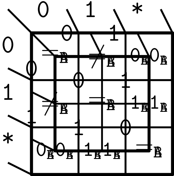
(b) Alice’s split gadget $g_{\mathsf{A}}$

(c) Bob’s split gadget $g_{\mathsf{B}}$

Figure 10: The matrices of the compatibility gadgets for the XOR and the split models.

It turns out that we can do the something similar in the split model, with a slight change. Instead of both players applying the same gadget on pairs of rows before testing for equality, they each apply a different gadget. The functions they apply bit-wise to pairs of rows are the transformations $g_{\mathsf{A}}$ and $g_{\mathsf{B}}$ represented in Figs. 10(b) and 10(c). The functions are chosen so that the following property holds.

Proposition D.2.

For all $X_{i}$, $X_{j}$, $Y_{i}$, and $Y_{j}\in\{0,1,*\}^{k}$, and $g_{\mathsf{A}},g_{\mathsf{B}}$ described in Figs. 10(b) and 10(c),

$$X_{i}\mathbin{{\mathsf{x\!x}}}Y_{i}=X_{j}\mathbin{{\mathsf{x\!x}}}Y_{j}\Leftrightarrow g_{\mathsf{A}}(X_{i},X_{j})=g_{\mathsf{B}}(Y_{i},Y_{j})$$

These functions capture when a pair of rows output the same result: if Alice outputs two stars in some position of $X_{i}$ and $X_{j}$, then Bob needs to be outputting two $0$s or two $1$s in the same position in his strings ($Y_{i}$ and $Y_{j}$). Similarly, if at some index Alice outputs a star in row $X_{i}$ and a $0$ in row $X_{j}$, then at this same index, Bob needs to output a $0$ in $Y_{i}$ and a star in $Y_{j}$ so that the two rows yield the same result.

Proposition D.2 implies that error-reduction in the split model reduces to solving $\mathbf{GapMAJ}$ combined with the weave gadget ($\mathbin{{\mathsf{x\!x}}}$), in the same way that error reduction in the XOR model reduced to solving $\mathbf{GapMAJ}{\circ}\mathbf{XOR}$. We obtain the following similar result Theorem D.3.

Theorem D.3.

Let $0<\epsilon^{\prime}<\epsilon<\frac{1}{2}$, $C_{\epsilon,\epsilon^{\prime}}=8\epsilon{\left\lparen\frac{1}{2}-\epsilon\right\rparen^{-2}}{\ln\left\lparen\frac{4}{\epsilon^{\prime}}\right\rparen}$. For all $f:\mathcal{X}\times\mathcal{Y}\rightarrow\{0,1\}^{k}$,

$$R^{\mathsf{spl}}_{\epsilon^{\prime}}(f)\leq C_{\epsilon,\epsilon^{\prime}}\cdot R^{\mathsf{spl}}_{\epsilon}(f)+O\left\lparen C_{\epsilon,\epsilon^{\prime}}\right\rparen.$$

Appendix E Error reduction for direct sum problems

This section gives the full proof of Theorem 5.8 which gives an error reduction scheme for functions of the form $f=g^{\otimes k}$.

Proof of Theorem 5.8.

Consider an XOR protocol for $f=g^{\otimes k}$ with error at most $\epsilon$, together with a protocol for $g$ with error at most $\epsilon$. The protocol to achieve error $\epsilon^{\prime}$ proceeds as follows.

Step 1:

[Restrict to at most two candidates.] The players run the XOR protocol for $f$ for a total of $T_{\epsilon^{\prime}}=50\ln\left\lparen\frac{12}{\epsilon^{\prime}}\right\rparen$ iterations. Let $(a_{i},b_{i})$ be what Alice and Bob would have output on the $i^{th}$ iteration. As in Step 1 of the proof of Theorem 5.6, with high probability, $\lvert\{i:a_{i}\oplus b_{i}=f(x,y)\}\rvert\geq\frac{2}{5}T_{\epsilon^{\prime}}$.

As in Step 2 of the proof of Theorem 5.6, the players then solve random $\mathbf{EQ}$ instances to find large subsets of iterations with the same computed value. With high probability ($\geq 1-\frac{\epsilon^{\prime}}{6}$), they compute at most $O(T_{\epsilon^{\prime}})$ instances of $\mathbf{EQ}$, with $\frac{\epsilon^{\prime}}{6}$ error.

With high probability ($\geq 1-3\cdot\frac{\epsilon^{\prime}}{6}$), the players should have identified either one or two sets of at least $\frac{11}{30}T_{\epsilon^{\prime}}$ iterations such that all iterations in a set computed the same value. If only one such large set was found, the players output $a_{i}$ and $b_{i}$ where $i$ is the index of an arbitrary iteration in this large set. Otherwise, let $i_{1}$ and $i_{2}$ be indices, each one representing one of the two large sets.

Step 2:

[Find a critical index $l$.] The players will either output as in the $i_{1}^{th}$ or the $i_{2}^{th}$ iteration. To decide between the two, they find the first difference between $a_{i_{1}}\oplus a_{i_{2}}$ and $b_{i_{1}}\oplus b_{i_{2}}$. This yields an index $l\in[k]$ where the two possible outputs differ. We call this a critical index.

Step 3.

[Solve GHD on the critical index $l$.] We XOR-compute the $l^{th}$ bit of $f$ $C_{\epsilon,\epsilon^{\prime}}$ times. This gives an instance of Gap Hamming Distance of size $C_{\epsilon,\epsilon^{\prime}}$ whose solution determines the $l^{th}$ bit of the correct output, with high probability. The players determine which iteration, $i_{1}$ or $i_{2}$, was correct on the $l^{th}$ bit, and output according to that iteration.

Altogether, we get the following upper bound on computing $f$ with error $\epsilon^{\prime}$.

$$R^{\mathsf{xor}}_{\epsilon^{\prime}}(f) \leq\left\lparen 50\ln\left\lparen\frac{12}{\epsilon^{\prime}}\right\rparen\right\rparen\cdot R^{\mathsf{xor}}_{\epsilon}(f)+R^{\mathsf{loc}}_{\epsilon^{\prime}/6}\left\lparen\mathbf{EQ}_{k}^{\otimes O(T_{\epsilon^{\prime}})}\right\rparen+R^{\mathsf{loc}}_{\epsilon^{\prime}/6}\left\lparen\mathbf{FtFD}_{k}\right\rparen$$

$$\qquad\quad+C_{\epsilon,\epsilon^{\prime}}\cdot R^{\mathsf{xor}}_{\epsilon}(g)+R^{\mathsf{loc}}_{\epsilon^{\prime}/6}\left\lparen\mathbf{GHD}^{C_{\epsilon,\epsilon^{\prime}}}_{(1/4+\epsilon/2)C_{\epsilon,\epsilon^{\prime}},(3/4-\epsilon/2)C_{\epsilon,\epsilon^{\prime}}}\right\rparen\ .$$

We conclude by applying known upper bounds for Find the First Difference [FRPU94] (Proposition 3.2), for solving many instances of Equality [FKNN95, Part 6] (Proposition 3.5), and Gap Hamming Distance is solved by exchanging the complete inputs which is essentially optimal [CR12, Vid12, She12]. ∎

Appendix F Removing randomness

F.1 Transcript Distribution Estimation

In this section we prove Lemmas 6.3 and F.1.

Proof of Lemma 6.3.

Let $\Pi$ be a communication protocol, and $\gamma=\delta\lvert\mathcal{T}_{\pi}\rvert^{-1}$. Given $(x,y)$, the players consider the protocol tree of $\Pi$ :

Figure 11: A tree representing the possible executions of the protocol $\Pi$ on a given $(x,y)$.

Each node of this tree represents a partial execution of the protocol, and so we label each node of this tree by the word $w\in\{0,1\}^{*}$ that is the communication that happened between Alice and Bob to reach this node. In particular, leaves are labeled by full transcripts, i.e., words $w\in\mathcal{T}_{\pi}$. We will use the notation $w_{<i}$ to refer to the prefix of $w$ of size $(i-1)$. Each internal node belongs to either Alice or Bob, and that property determines who must send the next message when at this specific point of the execution of the protocol. It has $\lvert\mathcal{T}_{\pi}\rvert$ leaves.

To each internal node $w$, we can assign a probability distribution $p_{w}$ that corresponds to which message ($0$ or $1$) is sent next. This distribution is fully determined by $x$ if the node belongs to Alice, by $y$ otherwise. Its randomness comes from the private randomness of the players, and its support is the set of next messages ($0$ or $1$ here). The probability that Alice sends $1$ as her next message when on node $w$ in the protocol tree is denoted by $p_{w}(1\mid x)$.

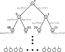
Figure 12: The same tree as in Fig. 11 with nodes labeled depending on their owners, and the probability distributions. Note that $p_{w}(0\mid x)+p_{w}(1\mid x)=1$.

For a leaf of label $w$, on input $(x,y)$, the probability that an execution of the protocol ends up in $w$ is:

$$p(w\mid x,y)=\underbrace{\left\lparen\prod_{\begin{subarray}{c}1\leq i\leq\lvert w\rvert\\ w_{<i}\in\textrm{Alice}\end{subarray}}p_{w_{<i}}(w_{i}\mid x)\right\rparen}_{\alpha(w\mid x)}\quad\times\quad\underbrace{\left\lparen\prod_{\begin{subarray}{c}1\leq i\leq\lvert w\rvert\\ w_{<i}\in\textrm{Bob}\end{subarray}}p_{w_{<i}}(w_{i}\mid y)\right\rparen}_{\beta(w\mid y)}.$$

For each $w\in\mathcal{T}_{\pi}$, Alice has full knowledge of $\alpha(w\mid x)$ and Bob has full knowledge of $\beta(w\mid y)$. We now describe the actual protocols in the Bob and in the open model.

Step 1.

For each $w\in\mathcal{T}_{\pi}$, Alice sends the smallest non-negative integer $d_{w}<\left\lceil\frac{1}{\gamma}\right\rceil$ such that:

$$\gamma\cdot d_{w}\leq\alpha(w\mid x)\leq\gamma\cdot(d_{w}+1).$$

This is done with communication $\lvert\mathcal{T}_{\pi}\rvert\cdot\left\lceil\log\frac{1}{\gamma}\right\rceil$.

Bob now knows an approximation $\alpha^{\prime}(w\mid x):=\gamma\cdot d_{w}$ of Alice’s $\alpha(w\mid x)$ for all $w$ such that:

$$\alpha^{\prime}(w\mid x)\leq\alpha(w\mid x)\leq\alpha^{\prime}(w\mid x)+\gamma.$$

Since $\beta(w\mid y)\in[0,1]$ for all $w$, $p^{\prime}(w\mid x,y):=\alpha^{\prime}(w\mid x)\beta(w\mid y)$ (known to Bob) is such that:

$$\forall w\in\mathcal{T}_{\pi}:p^{\prime}(w\mid x,y)\leq p(w\mid x,y)\leq p^{\prime}(w\mid x,y)+\gamma.$$

That is, Bob has an estimation of the true probabilities of $p(.\mid x,y)$ that never overestimates the true value and is pointwise $\gamma$-close to it.

Step 2.

Bob cannot simply output $p^{\prime}(.\mid x,y)$ since it might not be a probability distribution. However, $p(.\mid x,y)$ is a probability distribution, so:

$$1-\gamma\lvert\mathcal{T}_{\pi}\rvert\leq\sum_{w}p^{\prime}(w\mid x,y)\leq 1.$$

Let us define $C:=1-\sum_{w}p^{\prime}(w\mid x,y)$ and $p^{\prime\prime}(w\mid x,y)=p^{\prime}(w\mid x,y)+\frac{C}{\lvert\mathcal{T}_{\pi}\rvert}$ for all $w$. Since $0\leq C\leq\gamma\lvert\mathcal{T}_{\pi}\rvert$, $p^{\prime\prime}(.\mid x,y)$ is a distribution which is also a point-wise $\gamma$-approximation of $p(.\mid x,y)$. Our choice of $\gamma=\delta\lvert\mathcal{T}_{\pi}\rvert^{-1}$ makes $p^{\prime\prime}(.\mid x,y)$ $\delta$-close to $p(.\mid x,y)$ in statistical distance, so Bob can output it. Therefore

$$D^{\mathsf{B}}(\mathbf{TDE}_{\Pi,\delta})\leq\lvert\mathcal{T}_{\pi}\rvert\cdot\left\lceil\log\frac{\lvert\mathcal{T}_{\pi}\rvert}{\delta}\right\rceil\ .$$

which concludes the proof of Lemma 6.3.

∎

We will show a similar statement in the local and open models that we will use in proving other derandomization results.

Lemma F.1.

Let $\Pi$ be a private coin communication protocol and $\mathcal{T}_{\pi}$ its set of possible transcripts. For any $0<\delta<\frac{1}{2}$, $D^{\mathsf{loc}}(\mathbf{TDE}_{\Pi,\delta})\leq D^{\mathsf{open}}(\mathbf{TDE}_{\Pi,\delta})\leq 2\lvert\mathcal{T}_{\pi}\rvert\cdot\left\lceil\log\frac{2\lvert\mathcal{T}_{\pi}\rvert}{\delta}\right\rceil$.

Note that in the local model, we require that both players output the same approximation of the distribution on the leaves. In the original protocol of Lemma 6.3, it was enough for one player to send estimates and the other to use its exact values, but here, the second player must also send back the result. Hence, the protocol for $\mathbf{TDE}$ has slightly higher communication complexity in the local model than in the unilateral model.

In the local model, after running the protocol for $\mathbf{TDE}$, both players have the same estimate for the distribution over the leaves. Each player additionally knows her output distribution on each leaf, making the majority answer clear for both players. The situation is similar for an external observer in the open model after openly computing $\mathbf{TDE}$. Therefore, following, e.g., the proof of [KN97, Lemma 3.8], Lemma F.1 implies Theorem F.3.

Proof of Lemma F.1.

Let $\gamma=\frac{\delta}{2}\lvert\mathcal{T}_{\pi}\rvert^{-1}$. We proceed as in the proof of Lemma 6.3 but we replace the second step by the following one.

Step 2’.

Instead of outputting directly after the first step, Bob sends back an approximation of $p^{\prime}(.\mid x,y)$ to Alice. More precisely, for all $w$, he sends $d^{\prime}_{w},0\leq d^{\prime}_{w}<\left\lceil\frac{1}{\gamma}\right\rceil$ such that:

$$\gamma\cdot d^{\prime}_{w}\leq p^{\prime}(w\mid x,y)\leq\gamma\cdot(d^{\prime}_{w}+1).$$

This again takes communication $\lvert\mathcal{T}_{\pi}\rvert\cdot\left\lceil\log(\frac{1}{\gamma})\right\rceil$. Hence an external observer knows $p^{\prime\prime}(w\mid x,y):=\gamma\cdot d^{\prime}_{w}$ for all $w$, which satisfies:

$$\forall w\in\mathcal{T}_{\pi}:p^{\prime\prime}(w\mid x,y)\leq p(w\mid x,y)\leq p^{\prime\prime}(w\mid x,y)+2\cdot\gamma.$$

Let us define $C:=1-\sum_{w}p^{\prime\prime}(w\mid x,y)$ and $p^{\prime\prime\prime}(w\mid x,y)=p^{\prime\prime}(w\mid x,y)+\frac{C}{\lvert\mathcal{T}_{\pi}\rvert}$ for all $w$. This $p^{\prime\prime\prime}(.\mid x,y)$ is a distribution, and a $2\cdot\gamma$ point-wise approximation of $p(.\mid x,y)$, and can be computed by an external observer. By our choice of $\gamma=\frac{\delta}{2}\lvert\mathcal{T}_{\pi}\rvert^{-1}$, we get the output we want and so

$$D^{\mathsf{open}}(\mathbf{TDE}_{\Pi,\delta})\leq 2\lvert\mathcal{T}_{\pi}\rvert\cdot\left\lceil\log\frac{2\lvert\mathcal{T}_{\pi}\rvert}{\delta}\right\rceil,$$

which concludes the proof of Lemma F.1.

∎

F.2 Proof details for randomness removal (Section 6)

The following lemma will be useful in proving our results:

Lemma F.2.

Let $U$ and $V$ be random variables over their respective domain $\mathcal{U}$ and $\mathcal{V}$. For all $u\in\mathcal{U}$, le us consider $V_{U=u}$ the random variable $V$ conditioned on the event $[U=u]$. Assume there exists two constants $\delta_{U}$ and $\delta_{V}$ and two random variables $U^{\prime}$ and $V^{\prime}$ over the same domains as $U$ and $V$ such that:

$$\Delta(U,U^{\prime})\leq\delta_{U}\qquad\forall u\in\mathcal{U}:d_{\infty}(V_{U=u},V^{\prime}_{U^{\prime}=u})\leq\delta_{V}.$$

Then:

$$d_{\infty}(V,V^{\prime})\leq\delta_{U}+\delta_{V}.$$

Proof of Lemma F.2.

Let us show that $\forall v\in\mathcal{V}$, $\left\lvert\Pr[V=v]-\Pr[V^{\prime}=v]\right\rvert\leq\delta_{U}+\delta_{V}$. Fix an arbitrary $v\in\mathcal{V}$, then the probabilities $\Pr[V=v]$ and $\Pr[V^{\prime}=v]$ can be written as:

• $\Pr[V=v]=\sum_{u\in\mathcal{U}}\Pr[U=u]\cdot\Pr[V=v\mid U=u]$,

• $\Pr[V^{\prime}=v]=\sum_{u\in\mathcal{U}}\Pr[U^{\prime}=u]\cdot\Pr[V^{\prime}=v\mid U^{\prime}=u]$.

Hence using our two hypotheses above we get:

$$\Pr[V=v]-\Pr[V^{\prime}=v]$$

$$= \sum_{u\in\mathcal{U}}\left\lparen\Pr[U=u]\cdot\Pr[V=v\mid U=u]-\Pr[U^{\prime}=u]\cdot\Pr[V^{\prime}=v\mid U^{\prime}=u]\right\rparen$$

$$\leq \sum_{u\in\mathcal{U}}\left\lparen\left\lparen\Pr[U=u]-\Pr[U^{\prime}=u]\right\rparen\Pr[V=v\mid U=u]+\delta_{V}\Pr[U^{\prime}=u]\right\rparen$$

$$\leq \sum_{u\in\mathcal{U}:\Pr[U=u]>\Pr[U^{\prime}=u]}\left\lparen\Pr[U=u]-\Pr[U^{\prime}=u]\right\rparen+\delta_{V}$$

$$\leq \delta_{U}+\delta_{V}.$$

We can prove $\Pr[V=v]-\Pr[V^{\prime}=v]\geq-(\delta_{U}+\delta_{V})$ following the same proof method, and combining the two we get the desired result:

$$\forall v\in\mathcal{V}:\left\lvert\Pr[V=v]-\Pr[V^{\prime}=v]\right\rvert\leq\delta_{U}+\delta_{V}.$$

∎

F.3 Derandomization up to the XOR model

The open and local models are straightforward adaptations of Theorem 6.1.

Theorem F.3.

For any function $f$, error $\epsilon<\frac{1}{2}$ and model $\mathcal{M}\in\{\mathsf{open},\mathsf{loc}\}$, with $R^{\mathcal{M}}=R^{\mathcal{M},\mathsf{priv}}_{\epsilon}(f)$:

$$D^{\mathcal{M}}(f)\leq 2\cdot 2^{R^{\mathcal{M}}}\left\lparen R^{\mathcal{M}}+\log\left\lparen\tfrac{1}{\frac{1}{2}-\epsilon}\right\rparen+2\right\rparen$$

F.3.1 Derandomization in the one-out-of-two model

Interestingly, in the one-out-of-two model, there is an error threshold for derandomization at $\epsilon=\frac{1}{3}$. If the error is below this threshold, solving the appropriate instance of $\mathbf{TDE}$ suffices, after which one of the players knows the majority outcome. When the error is close to $1/2$, there can be several candidates for the majority outcome, which would cost an additional $O(k)$ to communicate. We reduce this term to $O(\log(k))$ in this case by using a variant of the NBA problem.

Theorem F.4.

For any function $f$ and error $\epsilon<\frac{1}{2}$, with $R=R^{\mathsf{1of2},\mathsf{priv}}_{\epsilon}(f)$:

$$D^{\mathsf{1of2}}(f)\leq\begin{cases}2^{R+1}\left\lparen R+\log\left\lparen\frac{4}{\frac{1}{3}-\epsilon}\right\rparen+1\right\rparen,&\text{if }\epsilon<\frac{1}{3},\\ \left\lparen 2^{R+1}+2\right\rparen\cdot\left\lparen R+\log\left\lparen\frac{8}{\frac{1}{2}-\epsilon}\right\rparen+1\right\rparen+\log(k)+4,&\text{for any }\epsilon<\frac{1}{2}.\end{cases}$$

Proof of Theorem F.4.

Take $\Pi$ to be an optimal private coin one-out-of-two protocol for $f$ with error $\epsilon$. Let $\sigma$ be a precision parameter which we will set later.

When $\epsilon<\frac{1}{3}$, notice that one of the players has to output the correct result with probability greater than $\frac{1}{3}$, while all incorrect ones are output with probability less than $\frac{1}{3}$ (with an additional small bias). So it suffices for the players to run the local protocol of Lemma F.1 for $\mathbf{TDE}_{\pi,\sigma}$ where $\sigma<\frac{1}{3}-\epsilon$ in this case, and let the player who outputs some result with probability greater than $\frac{1}{3}$ output it.

We now turn to the more interesting case where $1/3\leq\epsilon<\frac{1}{2}$. Let $\delta=\frac{1}{2}-\epsilon$ and $\sigma<\frac{\delta}{3}$. The players first run the local protocol for $\mathbf{TDE}_{\pi,\sigma}$, thus learning a $\sigma$ approximation of the probability of each transcript of the protocol. By Lemma F.2, since each player exactly knows her outputting distribution in each leaf, for all $z$, each player knows up to precision $\sigma$ her probability of outputting $z$ in the original protocol.

Let us call $p_{\mathsf{A}}^{z}$ the probability that Alice outputs $z$, and $\widetilde{p}_{\mathsf{A}}^{z}$ the approximation she has of it. For $z=f(x,y)$, we have $p_{\mathsf{A}}^{z}+p_{\mathsf{B}}^{z}\geq\frac{1}{2}+\delta$ and so $\widetilde{p}_{\mathsf{A}}^{z}+\widetilde{p}_{\mathsf{B}}^{z}\geq\frac{1}{2}+\delta-\sigma$.

Using this, the players consider some $z$ as candidates for $f(x,y)$. Alice considers $(z^{\mathsf{A}}_{i})_{i\in[n_{\mathsf{A}}]}$ the $n_{\mathsf{A}}$ answers $z$ such that $\widetilde{p}_{\mathsf{A}}^{z}\geq\frac{1}{4}+\frac{\delta-\sigma}{2}$. Similarly, Bob considers $(z^{\mathsf{B}}_{j})_{j\in[n_{\mathsf{B}}]}$ the $n_{\mathsf{B}}$ answers $z$ such that $\widetilde{p}_{\mathsf{B}}^{z}\geq\frac{1}{4}+\frac{\delta-\sigma}{2}$.

Since $\sum_{z}\widetilde{p}_{\mathsf{A}}^{z}+\widetilde{p}_{\mathsf{B}}^{z}=1$ (where the sum is over all $z\in\mathcal{Z}$), we have that: $n_{\mathsf{A}}+n_{\mathsf{B}}\leq 3$. Since the majority output represents strictly more than half of all ouputs we have $\max(n_{\mathsf{A}},n_{\mathsf{B}})\leq 2$.

The players use $4$ bits to send the values $n_{\mathsf{A}},n_{\mathsf{B}}$ to each other. Without loss of generality, assume $n_{\mathsf{A}}\geq n_{\mathsf{B}}$. Then four cases are possible:

1. $(n_{\mathsf{A}},n_{\mathsf{B}})=(1,0)$

2. $(n_{\mathsf{A}},n_{\mathsf{B}})=(2,1)$

3. $(n_{\mathsf{A}},n_{\mathsf{B}})=(2,0)$

4. $(n_{\mathsf{A}},n_{\mathsf{B}})=(1,1)$.

The first two cases are simple: if there is only one candidate (Item 1), the player who owns it outputs it. If there are three candidates (Item 2), the player with a single candidate outputs it knowing that it has to match one of the candidates on the other side and be the majority output.

For the remaining two cases, we will use a variant of the protocol for the NBA problem. For the case $(n_{\mathsf{A}},n_{\mathsf{B}})=(2,0)$, Alice (who has two candidates) sends to Bob the index of a bit where the two candidates differ, say $i\in[\lceil\log(\mathcal{Z})\rceil]$. Bob replies with $\sum_{z:z_{i}=0}\widetilde{p}_{\mathsf{B}}^{z}$. Alice can thus compute $\sum_{z:z_{i}=0}\widetilde{p}_{\mathsf{B}}^{z}+\widetilde{p}_{\mathsf{A}}^{z}$. If that quantity is greater than $\frac{1}{2}$, the correct candidate is the one whose $i$-th bit is $0$; otherwise, it is the other candidate.

Finally, let us consider the case $(n_{\mathsf{A}},n_{\mathsf{B}})=(1,1)$. Without loss of generality, assume Alice’s candidate, $z^{\mathsf{A}}_{1}$, is not correct, that is, $z^{\mathsf{A}}_{1}\neq f(x,y)=z^{\mathsf{B}}_{1}$. Then, we notice that the probability Alice outputting $z^{\mathsf{A}}_{1}$ and the probability of Bob outputting something different from $z^{\mathsf{B}}_{1}$ are less than $\epsilon=\frac{1}{2}-\delta$. To conclude the protocol, the players exchange $\widetilde{p}_{\mathsf{A}}^{z^{\mathsf{A}}_{1}}$ and $\widetilde{p}_{\mathsf{B}}^{z^{\mathsf{B}}_{1}}$ up to $\sigma$ precision. Then:

• $p_{\mathsf{B}}^{z^{\mathsf{B}}_{1}}+p_{\mathsf{B}}^{\top}-p_{\mathsf{A}}^{z^{\mathsf{A}}_{1}}=p_{\mathsf{B}}^{z^{\mathsf{B}}_{1}}+\sum_{z\neq z^{\mathsf{A}}_{1}}p_{\mathsf{A}}^{z}\geq p_{\mathsf{B}}^{z^{\mathsf{B}}_{1}}+p_{\mathsf{A}}^{z^{\mathsf{B}}_{1}}\geq\frac{1}{2}+\delta$,

• $p_{\mathsf{A}}^{z^{\mathsf{A}}_{1}}+p_{\mathsf{A}}^{\top}-p_{\mathsf{B}}^{z^{\mathsf{B}}_{1}}=p_{\mathsf{A}}^{z^{\mathsf{A}}_{1}}+\sum_{z\neq z^{\mathsf{B}}_{1}}p_{\mathsf{B}}^{z}\leq 1-p_{\mathsf{A}}^{z^{\mathsf{B}}_{1}}+p_{\mathsf{B}}^{z^{\mathsf{B}}_{1}}\leq\frac{1}{2}-\delta$.

Each player has a $\sigma$ approximation of the sum of probabilities of outputs on her side, and a $2\sigma$ approximation of the probability of the candidate output on the other player’s side, so they have a $3\sigma$ approximations of the above sums. Since $\sigma<\frac{\delta}{3}$, the players know with certainty if they have the correct output or not. If they do not have the correct output, they let the other player output. ∎

F.3.2 Derandomization in the split model

Derandomization in the split model can be achieved similarly to derandomization in the previously studied models.

Theorem F.5.

Let $0<\epsilon<1/2$ and $f:\mathcal{X}\times\mathcal{Y}\rightarrow\mathcal{Z}=\{0,1\}^{k}$. Let $R=R^{\mathsf{spl},\mathsf{priv}}_{\epsilon}(f)$, $M=16\cdot\left\lparen\frac{1}{2}-\epsilon\right\rparen^{-2}\cdot 2^{R}$. Then:

$$D^{\mathsf{spl}}(f)\leq\begin{cases}2^{R+1}\cdot\left\lparen R+\log\left\lparen\frac{4}{\frac{1}{3}-\epsilon}\right\rparen+1\right\rparen+k,&\text{if }\epsilon<\frac{1}{3},\\ 2^{R+1}\cdot\left\lparen R+\log\left\lparen\frac{8}{\frac{1}{2}-\epsilon}\right\rparen+1\right\rparen+k\cdot\left\lparen\frac{5-2\epsilon}{4}M+1\right\rparen,&\forall\epsilon<\frac{1}{2}.\end{cases}$$

Proof of Theorem F.5.

Case when $\epsilon<\frac{1}{3}$

As in the proof of Theorem F.4, for each string $z\in\{0,1,*\}^{k}$ the players estimate their probability of outputting $z$ by solving a $\mathbf{TDE}$ instance. For each index of the output, in the randomized protocol, one of the players has to output the correct bit with probability at least $\frac{1-\epsilon}{2}>\frac{1}{3}$. Alice sends $k$ bits to Bob to indicate for which bits she outputs the same non-$*$ symbol with probability more than $\frac{1}{3}$ in the original protocol. She outputs those bits in the derandomized protocol, while Bob is in charge of outputting the other bits. For each bit they output, they output the value which was most frequent in the original randomized protocol.

Case when $\epsilon<\frac{1}{2}$

This case is similar to what we saw in the proof of Theorem 6.4: we create a $\mathbf{GapMAJ}$ composed with the weave ($\mathbin{{\mathsf{x\!x}}}$) gadget, in the same way that we created a $\mathbf{GapMAJ}{\circ}\mathbf{XOR}$ instance to derandomize a protocol in the XOR model.

∎

As in the XOR model, these bounds can be improved by improving the deterministic complexity of the right gadgetized version of $\mathbf{GapMAJ}$ in the split model.

Appendix G Proofs of the bounds on $\mathbf{GapMAJ}{\circ}\mathbf{XOR}$

In this section we prove the statements of Table 2 about the communication complexity of $\mathbf{GapMAJ}{\circ}\mathbf{XOR}$.

Recall that the $\mathbf{GapMAJ}{\circ}\mathbf{XOR}$ problem is parameterized by four parameters: $N$ the number of rows, $k$ the length of Alice’s and Bob’s rows, $\epsilon$ the fraction of rows that do not XOR to the hidden $k$-bit string $z$, and $\mu$ a distribution over the rows. A $\mathbf{GapMAJ}{\circ}\mathbf{XOR}$ instance can be pictured as Alice and Bob each having a $N\times k$ boolean matrix such that the set of rows containing $z$ in the bitwise XOR of the two matrices has a weight higher than $1-\epsilon$ relative to $\mu$. In what follows, $\epsilon^{\prime}$ is the target probability, i.e., the maximal error rate we tolerate when solving our $\mathbf{GapMAJ}{\circ}\mathbf{XOR}$ instances.

When $\epsilon\leq\epsilon^{\prime}$, the trivial protocol in the XOR model which consists in choosing a row with public coins and outputting that row suffices. We thus have the following result.

Proposition G.1.

For all $N,k,\epsilon,\epsilon^{\prime},\mu$, with $0\leq\epsilon\leq\epsilon^{\prime}$,

$$R_{\epsilon^{\prime}}^{\mathsf{xor},\mathsf{pub}}(\mathbf{GapMAJ}_{N,k,\epsilon,\mu}{\circ}\mathbf{XOR})=0.$$

From this proposition we derive the following upper bounds.

Corollary G.2.

For all $N,k,\epsilon,\epsilon^{\prime},\mu$, with $0\leq\epsilon\leq\epsilon^{\prime}$

• $R_{\epsilon^{\prime}}^{\mathsf{xor},\mathsf{priv}}(\mathbf{GapMAJ}_{N,k,\epsilon,\mu}{\circ}\mathbf{XOR})\leq\log(N)$,

• $R_{\epsilon^{\prime}}^{\mathsf{open},\mathsf{pub}}(\mathbf{GapMAJ}_{N,k,\epsilon,\mu}{\circ}\mathbf{XOR})\leq 2k$,

• $R_{\epsilon^{\prime}}^{\mathsf{open},\mathsf{priv}}(\mathbf{GapMAJ}_{N,k,\epsilon,\mu}{\circ}\mathbf{XOR})\leq 2k+\log(N)$,

• $D^{\mathsf{uni}}(\mathbf{GapMAJ}_{N,k,\epsilon,\mu}{\circ}\mathbf{XOR})\leq(2\epsilon N+1)k$.

Proof of Corollary G.2.

The key is to notice that $\mathbf{GapMAJ}{\circ}\mathbf{XOR}$ is trivial when $\epsilon\leq\epsilon^{\prime}$ (Proposition G.1). For private coins, notice that the players only use $\log(N)$ coins, so it is enough for Alice (w.l.o.g.) to send her coins to Bob. For an open protocol, the players can exchange their rows. For the deterministic protocol, Alice (w.l.o.g.) sends her $(2\epsilon N+1)$ heaviest rows ($\mu$-wise) to Bob, who can then compute the most frequently occurring $z$ to which his rows and Alice’s rows XOR. ∎

When $\epsilon>\epsilon^{\prime}$, we refer to our earlier result from Section 5 (Theorem 5.6).

Appendix H Other separating problems

In this appendix, we give the definitions of the separating problems in Figs. 1 and 1 and prove that their complexity depends on the output model. All of them are variations of common problems with an additional constraint over the inputs, namely that at most $t$ bits of each player’s $n$-bit input are ones. Let us denote by $B_{2}(n,t)=\{x\in\{0,1\}^{n}:\sum_{i}x_{i}\leq t\}$ the Hamming ball of radius $t$ in $\{0,1\}^{n}$ centered at $0^{n}$, by $H(x)=-x\log(x)-(1-x)\log(1-x)$ the entropy of a Bernouilli random variable of expected value $x$, and recall the following bound on its size, which we denote by $V_{2}(n,t)=\lvert B_{2}(n,t)\rvert$:

Lemma H.1 (Chapter 10, Corollary 9 in [MS83]).

Let $0<t<n/2$. Then:

$$\frac{1}{\sqrt{8t(1-t/n)}}2^{n\cdot H(t/n)}\leq V_{2}(n,t)\leq 2^{n\cdot H(t/n)}.$$

In what follows, we will consider $t\in o(n)$, and only use that in this regime:

$$\log\lparen V_{2}(n,t)\rparen\in\Omega(t\cdot\log(n)).$$

H.1 $t$-Intersection

Since Disjointness is a Boolean problem, it cannot separate our models of communication. It is not the case, however, of its large-output variant Intersection, where Alice and Bob must compute the actual intersection of their sets.

We recall the definitions of the problems $t-\mathbf{DISJ}_{n}$ and $t-\mathbf{INT}_{n}$, what is known about their complexities, and show that $t-\mathbf{INT}_{n}$ separates the local model from the open model.

Definition H.2 ($t$-Disjointness problem).

$t-\mathbf{DISJ}_{n}:B_{2}(n,t)\times B_{2}(n,t)\rightarrow\{0,1\}$ is defined as:

$$t-\mathbf{DISJ}_{n}(X,Y)={\mathbf{1}}_{X\cap Y=\emptyset}.$$

We now define a natural variation of this problem, with large output.

Definition H.3 ($t$-Intersection problem).

$t-\mathbf{INT}_{n}:B_{2}(n,t)\times B_{2}(n,t)\rightarrow B_{2}(n,t)$ is defined as:

$$t-\mathbf{INT}_{n}(X,Y)=X\cap Y.$$

Since the output of $t-\mathbf{DISJ}_{n}$ is boolean, its various communication complexities are essentially the same up to one bit so we do not need to specify the communication model in the following statement:

Theorem H.4.

$R_{\epsilon}(t-\mathbf{DISJ}_{n})=\Theta(t).$

The $\Omega(t)$ lower bound comes directly from the $\Omega(n)$ lower bound for $\mathbf{DISJ}_{n}$ of [KS92, Raz92, BYJKS04], while the $O(k)$ upper bound was proven in [HW07].

Theorem H.5.

$R^{\mathsf{loc}}_{\epsilon}(t-\mathbf{INT}_{n})=\Theta(t)$, and $R^{\mathsf{open}}_{\epsilon}(t-\mathbf{INT}_{n})=\Theta(t\cdot\log(n)).$

The $O(t)$ upper bound for this problem was proved in [BCK⁺14] and the $\Omega(t\cdot\log(n))$ lower bound in the open model simply comes from the size of the output (Appendix C and Lemma H.1) since $\lvert B_{2}(n,t)\rvert=V_{2}(n,t)\in\Omega(t\cdot\log(n))$ (for $t\in o(n)$).

H.2 $t$-Find the First Difference

Just as Intersection can be seen as a large-output variant of the Disjointness problem, Find the First Difference can be thought of as the large-output variant of the Greater Than problem.

We now define the problems $t-\mathbf{GT}_{n}$ and $t-\mathbf{INT}_{n}$, what is known about their complexities, and show that $t-\mathbf{FtFD}_{n}$ separates the one-out-of-two model from the unilateral model.

Definition H.6 ($t$-Greater Than problem).

$t-\mathbf{GT}_{n}:B_{2}(n,t)\times B_{2}(n,t)\rightarrow\{0,1\}$ is defined as:

$$t-\mathbf{GT}_{n}(x,y)={\mathbf{1}}_{x>y}.$$

Definition H.7 ($t$-Find the First Difference problem).

$t{-}\mathbf{FtFD}_{n}:B_{2}(n,t)\times B_{2}(n,t)\rightarrow\{0,\ldots,n\}$ is defined as:

$$t-\mathbf{FtFD}_{n}(x,y)=\min\left\lparen\{i:x_{i}\neq y_{i}\}\cup\{n\}\right\rparen.$$

Theorem H.8.

$$R^{\mathsf{1of2}}_{\epsilon}(t-\mathbf{FtFD}_{n}) \in O\left\lparen\log(t)+\log(\log(n))+\log\left\lparen\frac{1}{\epsilon}\right\rparen\right\rparen,$$

$$R^{\mathsf{uni}}_{\epsilon}(t-\mathbf{FtFD}_{n}) \in\Omega(\log(n)).$$

Proof of Theorem H.8.

Upper bound on $R^{\mathsf{1of2}}_{\epsilon}(t-\mathbf{FtFD}_{n})$.

As an intuition, let us first give a protocol in the case $t=1$.

In this case, Alice and Bob $n$-bit strings $x$ and $y$ only contain a single $1$ each. So consider $i^{\mathsf{A}},i^{\mathsf{B}}$ such that $x_{i^{\mathsf{A}}}=1$ and $y_{i^{\mathsf{B}}}=1$. $i^{\mathsf{A}},i^{\mathsf{B}}\in[n]$, therefore they can be written as two $\lceil\log n\rceil$-bit strings.

The players then run the protocol of Feige et al [FRPU94] to find the first difference between $i^{\mathsf{A}}$ and $i^{\mathsf{B}}$. Doing so, they learn the smallest $t$ such that $(i^{\mathsf{A}})_{k}\neq(i^{\mathsf{B}})_{k}$ (or $\lceil\log(n)\rceil+1$ if it does not exist), and so whether $i^{\mathsf{A}}<i^{\mathsf{B}}$, $i^{\mathsf{A}}>i^{\mathsf{B}}$ or $i^{\mathsf{A}}=i^{\mathsf{B}}$. The player that has the lowest number thus knows the index of the first difference between $x$ and $y$, as it is $\min(i^{\mathsf{A}},i^{\mathsf{B}})$.

Now consider $t$ unconstrained. To find the first difference between their two $n$-bit strings of weight $\leq t$, the two players simply construct a $\Omega(t\cdot\log(n))$-bit string made of the indices of their $1$ bits (with adequate padding) and use the protocol of Feige et al [FRPU94] as in the $t=1$ case. More precisely:

• Let $w_{x}=\lvert x\rvert\leq t$ (resp. $w_{y}=\lvert y\rvert\leq t$) be the weight of $x$ (resp. $y$). Now, consider indices $i^{\mathsf{A}}_{1},\ldots,i^{\mathsf{A}}_{t}$ and $i^{\mathsf{B}}_{1},\ldots,i^{\mathsf{B}}_{t}$, in $\{0,\ldots,n-1\}\cup\{2^{\lceil\log(n+1)\rceil}-1\}$ such that:

  • $i^{\mathsf{A}}_{j}=2^{\lceil\log(n+1)\rceil}-1$ (an all-$1$ string) iff $j>w_{x}$

  • $x_{i^{\mathsf{A}}_{j}}=1,\forall j<=t$

  • $i^{\mathsf{A}}_{j}<i^{\mathsf{A}}_{j+1},\forall j<t$

    (and similarly for the $i^{\mathsf{B}}_{j}$’s)

  Each $i^{\mathsf{A}}_{j}$ can be written on $\lceil\log(n+1)\rceil$ bits, so Alice computes a $t\lceil\log n\rceil$-bit string $s_{x}$ made of the concatenation of all the $i^{\mathsf{A}}_{j}$’s, in order. Bob computes $s_{y}$ similarly.

  Then the two players use the protocol of Feige et al to obtain the first difference between $s_{x}$ and $s_{y}$. Let us note $i_{\mathsf{diff}}$ the index of this difference.

  Then Alice knows the index of the first difference if $(s_{x})_{i_{\mathsf{diff}}}=0$, and otherwise Bob does. Indeed, let us consider the first case:

  • The fact that there is a $0$ on this index for Alice means that this part of $s_{x}$ corresponds to the position of a $1$ in the original $n$-bit string $x$, since we pad with $1$’s at the end.

  • This position is the index of the leftmost $1$ that Alice has but Bob does not have. Indeed, all positions before the one $i_{\mathsf{diff}}$ belongs to are shared between Alice and Bob. So if Bob also had a $1$ in the position in which $i_{\mathsf{diff}}$ appears, then the fact that Alice and Bob find a difference in $i_{\mathsf{diff}}$ means that Bob also has a $1$ in a smaller position, which contradicts the fact that the first difference between $s_{x}$ and $s_{y}$ was such that Alice has a $0$ at that place.

  Using Feige et al’s protocol on a $O(t\cdot\log(n))$-bit string costs $O\left\lparen\log\left\lparen\frac{t\cdot\log(n)}{\epsilon}\right\rparen\right\rparen$, hence the advertised upper bound.

Lower bound on $R^{\mathsf{uni}}_{\epsilon}(t-\mathbf{FtFD}_{n})$.

Let Alice be the outputting player (w.l.o.g.), and consider inputs where she always receives the all-$0$ $n$-bit string and Bob receives a random $n$-bit string with a single $1$. Solving Find the First Difference on such instances would allow Bob to send an information of size $\log(n)$ bits to Alice with $R^{\mathsf{A}}_{\epsilon}(\mathbf{FtFD}_{n})$ communication and high probability, hence the $\Omega(\log(n))$ lower bound.

∎

Note that our one-out-of-two derandomization theorem (Theorem F.4) shows that our upper bound is tight for private coin communication complexity, but it may still be that there is a more efficient public coin protocol in the one-out-of-two or the XOR model. We now show that Viola’s $\Omega(\log(n))$ public coin randomized lower bound [Vio15] for $\mathbf{GT}_{n}$ implies that this protocol is also tight when given access to public coins.

Theorem H.9.

$$R_{\epsilon}(t-\mathbf{GT}_{n})\in\Omega(\log(t)+\log\log(n))$$

and as a corollary, $R_{\epsilon}^{\mathsf{xor}}(t-\mathbf{FtFD}_{n})\in\Omega(\log(t)+\log\log(n))$.

Proof of Theorem H.9.

We prove the dependencies in $\log(t)$ and in $\log\log(n)$ independently.

$R_{\epsilon}(t-\mathbf{GT}_{n})\in\Omega(\log(t))$.

We remark that $\mathbf{GT}_{t}$ reduces to $t-\mathbf{GT}_{n}$ in the same way that $\mathbf{DISJ}_{t}$ reduced to $t-\mathbf{DISJ}_{n}$ in the previous section, so applying Viola’s lower bound [Vio15] yields:

$$R_{\epsilon}(t-\mathbf{GT}_{n})\geq R_{\epsilon}(\mathbf{GT}_{t})\in\Omega(\log(t))$$

$R_{\epsilon}(t-\mathbf{GT}_{n})\in\Omega(\log\log(n))$.

We remark that $1-\mathbf{GT}_{n}$ reduces to $\mathbf{GT}_{\log(n)}$ since a way to compare two numbers with a single bit set to one in their binary representation is to compare the indices of the position of their single one. Hence, applying Viola’s lower bound [Vio15] again:

$$R_{\epsilon}(t-\mathbf{GT}_{n})\geq R_{\epsilon}(1-\mathbf{GT}_{n})\geq R_{\epsilon}(\mathbf{GT}_{\log(n)})\in\Omega(\log\log(n))$$

∎

H.3 The $\mathbf{MAX}$ problem

Definition H.10 (Maximum problem).

$\mathbf{MAX}_{n}:\{0,1\}^{n}\times\{0,1\}^{n}\rightarrow\{0,1\}^{n}$ is defined as

$$\mathbf{MAX}_{n}(x,y)=\begin{cases}x,&\text{if $x\geq y$,}\\ y,&\text{otherwise.}\end{cases}$$

For this problem, we have:

Theorem H.11.

$$R^{\mathsf{1of2}}_{\epsilon}(\mathbf{MAX}_{n})\in O(\log n),\qquad R^{\mathsf{uni}}_{\epsilon}(\mathbf{MAX}_{n})\in\Omega(n).$$

The gap is the same (asymptotically, up to multiplicative and additive constants) when only allowing private coins.

Proof of Theorem H.11.

$R^{\mathsf{1of2}}$ upper bound.

The players compute whether $x\leq y$ or not with high probability using $O(\log n)$ communication, then if $x\leq y$ Alice outputs $x$, otherwise Bob outputs $y$.

$R^{\mathsf{uni}}$ lower bound.

it suffices to show that $R^{\mathsf{A}}$ is large, as symmetry will imply that therefore $R^{\mathsf{B}}$ is large as well.

The proof is quite simple: consider the $2^{n}$ input pairs $\{(0,y):y\in[0,2^{n}-1]\}$. For those inputs, the $\mathbf{MAX}_{n}$ problem is just a problem of one-way communication: it is clear that he must send $\Omega(n)$ bits for Alice to correctly guess his $y$ with probability $\geq 1-\epsilon$.

∎

References

- [Aar05] Scott Aaronson. The complexity of agreement. In Proceedings of the thirty-seventh annual ACM symposium on Theory of computing, pages 634–643. ACM, 2005.
- [ABG+01] Andris Ambainis, Harry Buhrman, William Gasarch, Bala Kalyanasundaram, and Leen Torenvliet. The communication complexity of enumeration, elimination, and selection. Journal of Computer and System Sciences, 63(2):148–185, 2001.
- [BBCR13] Boaz Barak, Mark Braverman, Xi Chen, and Anup Rao. How to compress interactive communication. SIAM J. Comput., 42(3):1327—1363, 2013.
- [BBK+16] Joshua Brody, Harry Buhrman, Michal Koucký, Bruno Loff, Florian Speelman, and Nikolai K. Vereshchagin. Towards a reverse newman’s theorem in interactive information complexity. Algorithmica, 76(3):749–781, 2016.
- [BCK+14] Joshua Brody, Amit Chakrabarti, Ranganath Kondapally, David P. Woodruff, and Grigory Yaroslavtsev. Beyond set disjointness: the communication complexity of finding the intersection. In ACM Symposium on Principles of Distributed Computing, PODC ’14, pages 106–113, 2014.
- [BCK+16] Joshua Brody, Amit Chakrabarti, Ranganath Kondapally, David P. Woodruff, and Grigory Yaroslavtsev. Certifying equality with limited interaction. Algorithmica, 76(3):796–845, 2016.
- [BCMdW10] Harry Buhrman, Richard Cleve, Serge Massar, and Ronald de Wolf. Nonlocality and communication complexity. Rev. Mod. Phys., 82:665–698, Mar 2010.
- [BCW98] Harry Buhrman, Richard Cleve, and Avi Wigderson. Quantum vs. classical communication and computation. In Proceedings of the Thirtieth Annual ACM Symposium on Theory of Computing, pages 63–68. ACM, 1998.
- [BDKW14] Amos Beimel, Sebastian Ben Daniel, Eyal Kushilevitz, and Enav Weinreb. Choosing, agreeing, and eliminating in communication complexity. Comput. Complex., 23(1):1–42, 2014.
- [Bel64] J. S. Bell. On the Einstein Podolsky Rosen paradox. Physics, 1:195, 1964.
- [BK18] Mark Braverman and Gillat Kol. Interactive compression to external information. In Proceedings of the 50th Annual ACM SIGACT Symposium on Theory of Computing, STOC, pages 964–977, 2018.
- [BMY15] Balthazar Bauer, Shay Moran, and Amir Yehudayoff. Internal compression of protocols to entropy. In Approximation, Randomization, and Combinatorial Optimization. Algorithms and Techniques, APPROX/RANDOM 2015, pages 481–496, 2015.
- [Bol01] Béla Bollobás. Random Graphs. Cambridge Studies in Advanced Mathematics. Cambridge University Press, 2nd edition, 2001.
- [BR14] Mark Braverman and Anup Rao. Information equals amortized communication. IEEE Trans. Inf. Theory, 60(10):6058–6069, 2014.
- [Bra15] Mark Braverman. Interactive information complexity. SIAM J. Comput., 44(6):1698–1739, 2015.
- [BRWY13] Mark Braverman, Anup Rao, Omri Weinstein, and Amir Yehudayoff. Direct products in communication complexity. In 54th Annual IEEE Symposium on Foundations of Computer Science, FOCS 2013, 26-29 October, 2013, Berkeley, CA, USA, pages 746–755, 2013.
- [BYJKS04] Ziv Bar-Yossef, T. S. Jayram, Ravi Kumar, and D. Sivakumar. An information statistics approach to data stream and communication complexity. J. Comput. System Sci., 68(4):702–732, 2004.
- [CR12] Amit Chakrabarti and Oded Regev. An optimal lower bound on the communication complexity of gap-hamming-distance. SIAM J. Comput., 41(5):1299–1317, 2012.
- [ER60] Pál Erdős and Alfréd Rényi. On the evolution of random graphs. In Publication of the Mathematical Institute of the Hungarian Academy of Sciences, pages 17–61, 1960.
- [FJK+16] Lila Fontes, Rahul Jain, Iordanis Kerenidis, Sophie Laplante, Mathieu Laurière, and Jérémie Roland. Relative discrepancy does not separate information and communication complexity. ACM Trans. Comput. Theory, 9(1):4:1–4:15, 2016.
- [FKNN95] Tomas Feder, Eyal Kushilevitz, Moni Naor, and Noam Nisan. Amortized communication complexity. SIAM J. Comput., 24(4):736–750, August 1995.
- [FRPU94] Uriel Feige, Prabhakar Raghavan, David Peleg, and Eli Upfal. Computing with noisy information. SIAM J. Comput., 23(5):1001–1018, October 1994.
- [GKR16] Anat Ganor, Gillat Kol, and Ran Raz. Exponential separation of information and communication for boolean functions. J. ACM, 63(5):46:1–46:31, 2016.
- [GKR21] Anat Ganor, Gillat Kol, and Ran Raz. Exponential separation of communication and external information. SIAM J. Comput., 50(3), 2021.
- [HPZZ21] Dawei Huang, Seth Pettie, Yixiang Zhang, and Zhijun Zhang. The communication complexity of set intersection and multiple equality testing. SIAM J. Comput., 50(2):674–717, 2021.
- [HW07] Johan Håstad and Avi Wigderson. The randomized communication complexity of set disjointness. Theory of Computing, 3(11):211–219, 2007.
- [IW03] Piotr Indyk and David P. Woodruff. Tight lower bounds for the distinct elements problem. In Proc. 44th Symposium on Foundations of Computer Science (FOCS 2003), pages 283–288, 2003.
- [JK10] Rahul Jain and Hartmut Klauck. The partition bound for classical communication complexity and query complexity. In Proceedings of the 25th Annual IEEE Conference on Computational Complexity, CCC 2010, pages 247–258, 2010.
- [KN97] Eyal Kushilevitz and Noam Nisan. Communication Complexity. Cambridge University Press, New York, NY, USA, 1997.
- [Kol16] Gillat Kol. Interactive compression for product distributions. In Proceedings of the 48th Annual ACM SIGACT Symposium on Theory of Computing (STOC), pages 987–998. ACM, 2016.
- [Koz15] Alexander Kozachinskiy. Some bounds on communication complexity of gap hamming distance. CoRR, abs/1511.08854, 2015.
- [KS92] Bala Kalyanasundaram and Georg Schnitger. The probabilistic communication complexity of set intersection. SIAM J. Discrete Math., 5(4):545–557, 1992.
- [MS83] Florence Jessie MacWilliams and Neil James Alexander Sloane. Theory of Error-Correcting Codes, volume 16 of North-Holland Mathematical Library. Elsevier, 1983.
- [Nis93] Noam Nisan. The communication complexity of threshold gates. In Combinatorics, Paul Erdős is eighty, volume 1 of Bolyai Society Mathematical Studies, pages 301–315. János Bolyai Mathematical Society, 1993.
- [Orl90] Alon Orlitsky. Worst-case interactive communication I: two messages are almost optimal. IEEE Trans. Information Theory, 36(5):1111–1126, 1990.
- [Orl91] Alon Orlitsky. Worst-case interactive communication - II: two messages are not optimal. IEEE Trans. Information Theory, 37(4):995–1005, 1991.
- [PV16] Carlos Palazuelos and Thomas Vidick. Survey on nonlocal games and operator space theory. Journal of Mathematical Physics, 57(1):015220, 2016.
- [Raz92] Alexander A. Razborov. On the distributional complexity of disjointness. Theor. Comput. Sci., 106(2):385–390, 1992.
- [RS18] Anup Rao and Makrand Sinha. Simplified Separation of Information and Communication. Theory of Computing, 14(1):1–29, 2018.
- [RY20] Anup Rao and Amir Yehudayoff. Communication Complexity. Cambridge University Press, 2020.
- [She12] Alexander A. Sherstov. The communication complexity of gap hamming distance. Theory of Computing, 8(1):197–208, 2012.
- [She18] Alexander Sherstov. Compressing interactive communication under product distributions. SIAM J. Comput., 47(2):367–419, 2018.
- [Vid12] Thomas Vidick. A concentration inequality for the overlap of a vector on a large set, with application to the communication complexity of the gap-hamming-distance problem. Chicago J. Theor. Comput. Sci., 2012, 2012.
- [Vio15] Emanuele Viola. The communication complexity of addition. Combinatorica, 35(6):703–747, Dec 2015.
- [Wat18] Thomas Watson. Communication complexity with small advantage. In 33rd Computational Complexity Conference, CCC, pages 9:1–9:17, 2018.