Precoder Design for Massive MIMO Downlink with Matrix Manifold Optimization

Abstract

We investigate the weighted sum-rate (WSR) maximization linear precoder design for massive MIMO downlink and propose a unified matrix manifold optimization framework applicable to total power constraint (TPC), per-user power constraint (PUPC) and per-antenna power constraint (PAPC). Particularly, we prove that the precoders under TPC, PUPC and PAPC are on different Riemannian submanifolds, and transform the constrained problems in Euclidean space to unconstrained ones on manifolds. In accordance with this, we derive Riemannian ingredients including orthogonal projection, Riemannian gradient, Riemannian Hessian, retraction and vector transport, which are needed for precoder design in matrix manifold framework. Then, Riemannian design methods using Riemannian steepest descent, Riemannian conjugate gradient and Riemannian trust region are provided to design the WSR-maximization precoders under TPC, PUPC or PAPC. Riemannian methods are free of the inverse of large dimensional matrix, which is of great significance for practice. Complexity analysis and performance simulations demonstrate the advantages of the proposed precoder design.

I Introduction

Massive multiple-input multiple-output (MIMO) is one of the key techniques in the fifth generation (5G) wireless networks and will play a key role in future 6G systems with further increased antenna number scale [1, 2]. In massive MIMO systems, the base station (BS) equipped with a large number of antennas can serve a number of user terminals (UT) on the same time-frequency resource, providing enormous potential capacity gains and high energy efficiency [3, 4]. However, serving many users simultaneously causes serious inter-user interference, which may reduce the throughput. To suppress the interference and increase the system throughput, precoders should be properly designed for massive MIMO downlink (DL) transmission. Specifically, a linear precoder is particularly attractive due to its low complexity [5, 6, 7].

There are several criteria for the DL precoder design, including minimum mean square error (MMSE), weighted sum rate (WSR), quality of service (QoS), signal-to-interference-plus-noise ratio (SINR), signal-to-leakage-and-noise ratio (SLNR), energy efficiency (EE), etc. [8, 9, 10, 11, 12, 13]. Among these criteria, WSR is of great practical significance and widely considered in massive MIMO systems, as it directly aims at increasing the system throughput, which is one of the main objectives of communication systems. In addition, different power constraints may be imposed to the designs. Generally, power constraints for massive MIMO systems can be classified into three main categories: total power constraint (TPC), per-user power constraint (PUPC) and per-antenna power constraint (PAPC). Designing precoders under different power constraints usually forms different problems, for which different approaches are proposed in the literature. More specifically, the precoder design problem under TPC is typically formulated as a non-convex WSR-maximization problem, which is transformed into an MMSE problem iteratively solved by alternating optimization in [9]. Alternatively, [14] solves the WSR-maximization problem in the framework of the minorization-maximization (MM) method by finding a surrogate function of the objective function. When designing precoders under PUPC, the received SINR of each user is usually investigated with QoS constraints. With the received SINR, the sum-rate maximization problem is formulated and solved by Lagrange dual function [15, 11]. Precoders under PAPC are deeply coupled with each other and thus challenging to design. In [16] and [17], precoders under PAPC are designed by forcing precoders under TPC to satisfy PAPC or minimizing the distance between the precoders under TPC and those under PAPC .

In general, the designs of WSR-maximization precoders under the power constraints mentioned above can be formulated as optimization problems with equality constraints. Recently, manifold optimization has been extensively studied and successfully applied to many domains [18, 19, 20, 21], showing a great advantage in dealing with the challenging equality constraints. In mathematics, a manifold is a topological space that locally resembles Euclidean space near each point. By revealing the inherent geometric properties of the equality constraints, manifold optimization reformulates the constrained problems in Euclidean space as unconstrained ones on manifold. By defining the Riemannian ingredients associated with a Riemannian manifold, several Riemannian methods are presented for solving the unconstrained problems on manifold. In addition, manifold optimization usually shows promising algorithms resulting from the combination of insight from differential geometry, optimization, and numerical analysis. Therefore, manifold optimization can provide a potential way for designing optimal WSR-maximization precoders under different power constraints in a unified framework.

In this paper, we focus on WSR-maximization precoder design and propose for massive MIMO DL transmission a matrix manifold framework applicable to TPC, PUPC and PAPC. We reveal the geometric properties of the precoders under different power constraints and prove that the precoder sets satisfying TPC, PUPC and PAPC form three different Riemannian submanifolds, respectively, transforming the constrained problems in Euclidean space into unconstrained ones on manifold. To facilitate a better understanding, we analyze the precoder designs under TPC, PUPC and PAPC in detail. All the ingredients required during the optimizations on Riemannian submanifolds are derived for the three power constraints. Further, we present three Riemannian design methods using Riemannian steepest descent (RSD), Riemannian conjugate gradient (RCG) and Riemannian trust region (RTR), respectively. Riemannian methods are free of the inverse of large dimensional matrix, which is of great significance for practice. Complexity analysis shows that the method using RCG is computationally efficient. The numerical results confirm the performance advantages.

The remainder of the paper is organized as follows. In Section II, we introduce the preliminaries in matrix manifold optimization. In Section III, we first formulate the WSR-maximization precoder design problem in Euclidean space. Then we transform the constrained problems in Euclidean space under TPC, PUPC and PAPC to the unconstrained ones on Riemannian submanifolds and derive Riemannian ingredients in the matrix manifold framework. To solve the unconstrained problems on the Riemannian submanifolds, Section IV provides three Riemannian design methods and their complexity analyses. Section V presents numerical results and discusses the performance of the proposed precoder designs. The conclusion is drawn in Section VI.

Notations: Boldface lowercase and uppercase letters represent the column vectors and matrices, respectively. We write conjugate transpose of matrix $\mathbf{A}$ as $\mathbf{A}^{H}$ while $\mathrm{tr}\left(\mathbf{A}\right)$ and $\det\left(\mathbf{A}\right)$ denote the matrix trace and determinant of $\mathbf{A}$, respectively. $\Re\left\{\mathbf{A}\right\}$ means the real part of $\mathbf{A}$. Let the mathematical expectation be $\mathbb{E}\left\{\cdot\right\}$. $\mathbf{I}_{M}$ denotes the $M\times M$ dimensional identity matrix, whose subscript may be omitted for brevity. $\mathbf{0}$ represents the vector or matrix whose elements are all zero. The Hadamard product of $\mathbf{A}$ and $\mathbf{B}$ is $\mathbf{A}\odot\mathbf{B}$. Let $\mathbf{e}_{j}$ denote the vector with the $j$-th element equals $1$ while the others equal $0$. $\mathrm{diag}\left(\mathbf{b}\right)$ represents the diagonal matrix with $\mathbf{b}$ along its main diagonal and $\mathrm{diag}\left(\mathbf{A}\right)$ denotes the column vector of the main diagonal of $\mathbf{A}$. Similarly, $\mathbf{D}=\mathrm{blkdiag}\left\{\mathbf{A}_{1},\cdots,\mathbf{A}_{K}\right\}$ denotes the block diagonal matrix with $\mathbf{A}_{1},\cdots,\mathbf{A}_{K}$ on the diagonal and $\left[\mathbf{D}\right]_{i}$ denotes the $i$-th matrix on the diagonal, i.e., $\mathbf{A}_{i}$. A mapping $F$ from manifold $\mathcal{M}$ to manifold $\mathcal{N}$ is $F:\mathcal{M}\rightarrow\mathcal{N}:\mathbf{X}\mapsto\mathbf{Y}$ denoted as $F(\mathbf{X})=\mathbf{Y}$. The differential of $F\left(\mathbf{X}\right)$ is represented as $\mathrm{D}F\left(\mathbf{X}\right)$ while $\mathrm{D}F\left(\mathbf{X}\right)\left[{\boldsymbol{\xi}}_{\mathbf{X}}\right]$ or $\mathrm{D}F\left[{\boldsymbol{\xi}}_{\mathbf{X}}\right]$ means the directional derivative of $F$ at $\mathbf{X}$ along the tangent vector ${\boldsymbol{\xi}}_{\mathbf{X}}$.

II Preliminaries for Matrix Manifold Optimization

We introduce some basic notions in matrix manifold optimization in this section and list some common notations in Table I, with $\overline{\mathcal{M}}$ representing a Riemannian manifold. To avoid overwhelmingly redundant preliminaries, we focus on a coordinate-free analysis and omit charts and differential structures. For a full introduction to smooth manifolds, we refer to references [22, 23, 24].

TABLE I: Notations of the ingredients on a Riemannian submanifold $\overline{\mathcal{M}}$

$\bar{\mathbf{X}}$	A point on $\overline{\mathcal{M}}$	$T_{\bar{\mathbf{X}}}\overline{\mathcal{M}}$	Tangent space of $\overline{\mathcal{M}}$ at $\bar{\mathbf{X}}$
${\boldsymbol{\xi}}_{\bar{\mathbf{X}}}$	Tangent vector in $T_{\bar{\mathbf{X}}}\overline{\mathcal{M}}$	$N_{\bar{\mathbf{X}}}\overline{\mathcal{M}}$	Normal space of $\overline{\mathcal{M}}$ at $\bar{\mathbf{X}}$
$f(\bar{\mathbf{X}})$	Smooth function defined on $\overline{\mathcal{M}}$	$\mathrm{D}f\left(\bar{\mathbf{X}}\right)\left[\cdot\right]$	Differential operator of $f\left(\bar{\mathbf{X}}\right)$
$g_{\bar{\mathbf{X}}}\left(\cdot\right)$	Riemannian metric operator on $T_{\bar{\mathbf{X}}}\overline{\mathcal{M}}$	$R_{\bar{\mathbf{X}}}\left(\cdot\right)$	Retraction operator from $T_{\bar{\mathbf{X}}}\overline{\mathcal{M}}$ to $\overline{\mathcal{M}}$
$\mathrm{grad}f(\bar{\mathbf{X}})$	Riemannian gradient of $f(\bar{\mathbf{X}})$	$\mathrm{Hess}f(\bar{\mathbf{X}})\left[\cdot\right]$	Riemannian Hessian operator of $f(\bar{\mathbf{X}})$
${\boldsymbol{\Pi}}_{T_{\bar{\mathbf{X}}}{\overline{\mathcal{M}}}}^{T_{\mathbf{X}}{\mathcal{M}}}\left({\boldsymbol{\xi}}_{\mathbf{X}}\right)$	Orthogonal projection from $T_{\mathbf{X}}{\mathcal{M}}$ to $T_{\bar{\mathbf{X}}}{\overline{\mathcal{M}}}$	$\mathcal{T}_{\eta_{\bar{\mathbf{X}}}}\left(\cdot\right)$	Vector transport operator to $T_{R_{\bar{\mathbf{X}}}\left(\eta_{\bar{\mathbf{X}}}\right)}\overline{\mathcal{M}}$

For a manifold $\mathcal{M}$, a smooth mapping $\gamma:\mathbb{R}\rightarrow\mathcal{M}:t\mapsto\gamma(t)$ is termed a curve in $\mathcal{M}$. Let $\mathbf{X}$ be a point on $\mathcal{M}$ and $\mathcal{F}_{\mathbf{X}}(\mathcal{M})$ denote the set of smooth real-valued functions defined on a neighborhood of $\mathbf{X}$. A tangent vector ${\boldsymbol{\xi}}_{\mathbf{X}}$ to a manifold $\mathcal{M}$ at a point $\mathbf{X}$ is a mapping from $\mathcal{F}_{\mathbf{X}}(\mathcal{M})$ to $\mathbb{R}$ such that there exists a curve $\gamma$ on $\mathcal{M}$ with $\gamma(0)=\mathbf{X}$, satisfying ${\boldsymbol{\xi}}_{\mathbf{X}}f=\left.\frac{\mathrm{d}(f(\gamma(t)))}{\mathrm{d}t}\right|_{t=0}$ for all $f\in\mathcal{F}_{\mathbf{X}}(\mathcal{M})$. Such a curve $\gamma$ is said to realize the tangent vector ${\boldsymbol{\xi}}_{\mathbf{X}}$. For a manifold $\mathcal{M}$, every point $\mathbf{X}$ on the manifold is attached to a unique and linear tangent space, denoted by $T_{\mathbf{X}}\mathcal{M}$. $T_{\mathbf{X}}\mathcal{M}$ is a set of all the tangent vectors to $\mathcal{M}$ at $\mathbf{X}$. The tangent bundle is the set of all tangent vectors to $\mathcal{M}$ denoted by $T\mathcal{M}$, which is also a manifold. A vector field ${\boldsymbol{\xi}}$ on a manifold $\mathcal{M}$ is a smooth mapping from $\mathcal{M}$ to $T\mathcal{M}$ that assigns to each point $\mathbf{X}\in\mathcal{M}$ a tangent vector ${\boldsymbol{\xi}}_{\mathbf{X}}\in T_{\mathbf{X}}\mathcal{M}$. Particularly, every vector space $\mathcal{E}$ forms a linear manifold naturally. Assuming $\mathcal{M}$ is a vector space $\mathcal{E}$, we have $T_{\mathbf{X}}\mathcal{M}=\mathcal{E}$.

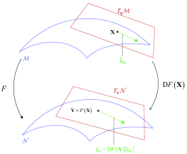
Figure 1: The relationship between two manifolds. $F$ is a linear mapping from $\mathcal{M}$ to $\mathcal{N}$, and $\mathrm{D}F\left(\mathbf{X}\right)$ is a linear mapping from $T_{\mathbf{X}}{\mathcal{M}}$ to $T_{\mathbf{Y}}{\mathcal{N}}$.

Let $F:\mathcal{M}\rightarrow\mathcal{N}$ be a smooth mapping from manifold $\mathcal{M}$ to manifold $\mathcal{N}$. The differential of $F$ at $\mathbf{X}$ is a linear mapping from $T_{\mathbf{X}}\mathcal{M}$ to $T_{\mathbf{Y}}\mathcal{N}$, denoted by $\mathrm{D}F\left(\mathbf{X}\right)\left[\cdot\right]$. Denote $\mathbf{Y}=F\left(\mathbf{X}\right)$ as a point on $\mathcal{N}$. Similarly, ${\boldsymbol{\xi}}_{\mathbf{Y}}=\mathrm{D}F\left(\mathbf{X}\right)\left[{\boldsymbol{\xi}}_{\mathbf{X}}\right]$ is a tangent vector to $\mathcal{N}$ at $\mathbf{Y}$, i.e., an element in $T_{\mathbf{Y}}\mathcal{N}$. In particular, if $\mathcal{M}$ and $\mathcal{N}$ are linear manifolds, $\mathrm{D}F\left(\mathbf{X}\right)$ reduces to the classical directional derivative [25]

$$\mathrm{D}F\left(\mathbf{X}\right)\left[\boldsymbol{{\boldsymbol{\xi}}}_{\mathbf{X}}\right]=\lim_{t\rightarrow 0}\frac{F\left(\mathbf{X}+t\boldsymbol{{\boldsymbol{\xi}}}_{\mathbf{X}}\right)-F\left(\mathbf{X}\right)}{t}.$$ (1)

The rank of $F$ at $\mathbf{X}$ is the dimension of the range of $\mathrm{D}F\left(\mathbf{X}\right)\left[\boldsymbol{{\boldsymbol{\xi}}}_{\mathbf{X}}\right]$. Fig. 1 is a simple illustration for geometric understanding. In practice, the equality constraint in many optimization problems forms a mapping between two linear manifolds. The solutions satisfying an equality constraint constitute a set $\overline{\mathcal{M}}=\left\{\mathbf{X}\in\mathcal{M}\mid F(\mathbf{X})=0\right\}$. The set $\overline{\mathcal{M}}$ may admit several manifold structures, while it admits at most one differential structure that makes it an embedded submanifold of $\mathcal{M}$. Whether $\overline{\mathcal{M}}$ forms an embedded submanifold mainly depends on the properties of $F\left(\mathbf{X}\right)$ [22, Proposition 3.3.2]. We assume $\overline{\mathcal{M}}$ is an embedded submanifold of $\mathcal{M}$ in the rest of this section to facilitate the introduction. Let $\bar{\mathbf{X}}\in\overline{\mathcal{M}}$ represent $\mathbf{X}\in\mathcal{M}$ that satisfies $F\left(\mathbf{X}\right)=0$ to distinguish it from $\mathbf{X}$. A level set of a real-valued function $F$ is the set of values $\mathbf{X}$ for which $F\left({\mathbf{X}}\right)$ is equal to a given constant. In particular, when $\overline{\mathcal{M}}$ is defined as a level set of a constant-rank function $F$, the tangent space of $\overline{\mathcal{M}}$ at $\bar{\mathbf{X}}$ is the kernel of the differential of $F$ and a subspace of the tangent space of $\mathcal{M}$:

$$T_{\bar{\mathbf{X}}}{\overline{\mathcal{M}}}=\mathrm{ker}\left(\mathrm{D}F\left(\mathbf{X}\right)\right)\subseteq T_{\mathbf{X}}\mathcal{M}.$$ (2)

By endowing tangent space with an inner product $g_{\mathbf{X}}\left(\cdot\right)$, we can define the length of tangent vectors in $T_{\mathbf{X}}\mathcal{M}$. Note that the subscript $\mathbf{X}$ in $g_{\mathbf{X}}\left(\cdot\right)$ is also used to distinguish the metric of different points on different manifolds for clarity. $g_{\mathbf{X}}\left(\cdot\right)$ is called Riemannian metric if it varies smoothly and the manifold is called Riemannian manifold. Since $T_{\bar{\mathbf{X}}}{\overline{\mathcal{M}}}$ can be regarded as a subspace of $T_{\mathbf{X}}{\mathcal{M}}$, the Riemannian metric $g_{\mathbf{X}}\left(\cdot\right)$ on $\mathcal{M}$ induces a Riemannian metric $g_{\bar{\mathbf{X}}}\left(\cdot\right)$ on $\overline{\mathcal{M}}$ according to

$$g_{\bar{\mathbf{X}}}\left({\boldsymbol{\xi}}_{\bar{\mathbf{X}}},{\boldsymbol{\zeta}}_{\bar{\mathbf{X}}}\right)=g_{\mathbf{X}}\left({\boldsymbol{\xi}}_{\bar{\mathbf{X}}},{\boldsymbol{\zeta}}_{\bar{\mathbf{X}}}\right).$$ (3)

Note that ${\boldsymbol{\xi}}_{\bar{\mathbf{X}}}$ and ${\boldsymbol{\zeta}}_{\bar{\mathbf{X}}}$ on the right hand side are viewed as elements in $T_{\mathbf{X}}\mathcal{M}$. Endowed with the Riemannian metric (3), the embedded submanifold $\overline{\mathcal{M}}$ forms a Riemannian submanifold.

In practice, it is suggested to utilize the orthogonal projection to obtain the elements in $T_{\bar{\mathbf{X}}}{\overline{\mathcal{M}}}$. With the Riemannian metric $g_{\mathbf{X}}\left(\cdot\right)$, the $T_{\mathbf{X}}{\mathcal{M}}$ can be divided into two orthogonal subspaces as

$$T_{\mathbf{X}}{\mathcal{M}}=T_{\bar{\mathbf{X}}}{\overline{\mathcal{M}}}\oplus N_{\bar{\mathbf{X}}}{\overline{\mathcal{M}}},$$ (4)

where the normal space $N_{\bar{\mathbf{X}}}{\overline{\mathcal{M}}}$ is the orthogonal complement of $T_{\bar{\mathbf{X}}}{\overline{\mathcal{M}}}$ defined as

$$N_{\bar{\mathbf{X}}}{\overline{\mathcal{M}}}=\left\{{\boldsymbol{\xi}}_{\mathbf{X}}\in T_{\mathbf{X}}\mathcal{M}\mid g_{\mathbf{X}}\left({\boldsymbol{\xi}}_{\mathbf{X}},{\boldsymbol{\zeta}}_{\bar{\mathbf{X}}}\right)=0,\ \forall{\boldsymbol{\zeta}}_{\bar{\mathbf{X}}}\in T_{\bar{\mathbf{X}}}{\overline{\mathcal{M}}}\right\}.$$ (5)

Thus, any ${\boldsymbol{\xi}}_{\mathbf{X}}\in T_{\mathbf{X}}{\mathcal{M}}$ can be uniquely decomposed into the sum of an element in $T_{\bar{\mathbf{X}}}{\overline{\mathcal{M}}}$ and an element in $N_{\bar{\mathbf{X}}}{\overline{\mathcal{M}}}$

$${\boldsymbol{\xi}}_{\mathbf{X}}={\boldsymbol{\Pi}}_{T_{\bar{\mathbf{X}}}{\overline{\mathcal{M}}}}^{T_{\mathbf{X}}{\mathcal{M}}}\left({\boldsymbol{\xi}}_{\mathbf{X}}\right)+{\boldsymbol{\Pi}}_{N_{\bar{\mathbf{X}}}{\overline{\mathcal{M}}}}^{T_{\mathbf{X}}{\mathcal{M}}}\left({\boldsymbol{\xi}}_{\mathbf{X}}\right),$$ (6)

where ${\boldsymbol{\Pi}}_{\mathbf{B}}^{\mathbf{A}}\left(\cdot\right)$ denotes the orthogonal projection from $\mathbf{A}$ to $\mathbf{B}$.

For a smooth real-valued function $f$ on a Riemannian submanifold $\overline{\mathcal{M}}$, the Riemannian gradient of $f$ at $\bar{\mathbf{X}}$, denoted by $\mathrm{grad}f(\bar{\mathbf{X}})$, is defined as the unique element in $T_{\bar{\mathbf{X}}}{\overline{\mathcal{M}}}$ that satisfies

$$g_{\bar{\mathbf{X}}}\left(\mathrm{grad}f(\bar{\mathbf{X}}),\boldsymbol{{\boldsymbol{\xi}}}_{\bar{\mathbf{X}}}\right)=\mathrm{D}f\left(\bar{\mathbf{X}}\right)\left[\boldsymbol{{\boldsymbol{\xi}}}_{\bar{\mathbf{X}}}\right],\forall{\boldsymbol{\xi}}_{\bar{\mathbf{X}}}\in T_{\bar{\mathbf{X}}}\overline{\mathcal{M}}.$$ (7)

Denote $\mathrm{grad}f$ as the vector field of the Riemannian gradient. Note that, since $\mathrm{grad}f(\bar{\mathbf{X}})\in T_{\bar{\mathbf{X}}}{\overline{\mathcal{M}}}$, we have $\mathrm{grad}f(\mathbf{X})\in T_{\mathbf{X}}\mathcal{M}$ and it can then be decomposed as (6).

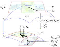
Figure 2: Geometric interpretation of orthogonal projection, retraction and vector transport.

When second-order derivative optimization algorithms, such as Newton method and trust-region method, are preferred, affine connection is indispensable [22]. Let $\mathfrak{X}(\mathcal{M})$ denote the set of smooth vector fields on $\mathcal{M}$, the affine connection on $\mathcal{M}$ is defined as a mapping $\nabla^{\mathcal{M}}:\mathfrak{X}(\mathcal{M})\times\mathfrak{X}(\mathcal{M})\rightarrow\mathfrak{X}(\mathcal{M}):(\boldsymbol{\eta},\boldsymbol{{\boldsymbol{\xi}}})\mapsto\nabla_{\boldsymbol{\eta}}^{\mathcal{M}}\boldsymbol{{\boldsymbol{\xi}}}$. When Riemannian manifold $\overline{\mathcal{M}}$ is an embedded submanifold of a vector space, $\nabla_{\boldsymbol{\eta}_{\bar{\mathbf{X}}}}^{\overline{\mathcal{M}}}\bar{{\boldsymbol{\xi}}}$ is called Riemannian connection and given as [22, Proposition 5.3.1]

$$\nabla_{\boldsymbol{\eta}_{\bar{\mathbf{X}}}}^{\overline{\mathcal{M}}}\bar{{\boldsymbol{\xi}}}= {\boldsymbol{\Pi}}_{T_{\bar{\mathbf{X}}}{\overline{\mathcal{M}}}}^{T_{\mathbf{X}}{\mathcal{M}}}\left(\nabla_{\boldsymbol{\eta}_{{\bar{\mathbf{X}}}}}^{\mathcal{M}}\bar{{\boldsymbol{\xi}}}\right)$$ (8)

$$= {\boldsymbol{\Pi}}_{T_{\bar{\mathbf{X}}}{\overline{\mathcal{M}}}}^{T_{\mathbf{X}}{\mathcal{M}}}\left(\mathrm{D}\bar{\boldsymbol{{\boldsymbol{\xi}}}}\left[\boldsymbol{\eta}_{{\bar{\mathbf{X}}}}\right]\right),\forall\boldsymbol{\eta}_{\bar{\mathbf{X}}}\in T_{\bar{\mathbf{X}}}\overline{\mathcal{M}},\bar{{\boldsymbol{\xi}}}\in\mathfrak{X}(\overline{\mathcal{M}}).$$

Given a Riemannian connection $\nabla^{\overline{\mathcal{M}}}$ defined on $\overline{\mathcal{M}}$, the Riemannian Hessian of a real valued function $f$ at point $\bar{\mathbf{X}}$ on $\overline{\mathcal{M}}$ is the linear mapping $\operatorname{Hess}f(\mathbf{\bar{X}})\left[\cdot\right]$ of $T_{\bar{\mathbf{X}}}\overline{\mathcal{M}}$ into itself defined as

$$\mathrm{Hess}f(\bar{\mathbf{X}})\left[\boldsymbol{{\boldsymbol{\xi}}}_{\bar{\mathbf{X}}}\right]=\nabla_{\boldsymbol{{\boldsymbol{\xi}}}_{\bar{\mathbf{X}}}}^{\overline{\mathcal{M}}}\mathrm{grad}f.$$ (9)

The notion of moving along the tangent vector while remaining on the manifold is generalized by retraction. The retraction $R_{\mathbf{X}}\left(\cdot\right)$, a smooth mapping from $T_{\mathbf{X}}\mathcal{M}$ to $\mathcal{M}$ [22, Definition 4.1.1], builds a bridge between the linear $T_{\mathbf{X}}\mathcal{M}$ and the nonlinear $\mathcal{M}$. Practically, the Riemannian exponential mapping forms a retraction but is computationally expensive to implement. For a Riemannian submanifold $\overline{\mathcal{M}}$, the geometric structure of the manifold is utilized to define the retraction $R_{\bar{\mathbf{X}}}\left(\cdot\right)$ through projection for affordable and efficient access.

Sometimes we need to move the tangent vector from the current tangent space to another, which is not always straightforward as the tangent spaces are different in a nonlinear manifold. To address this difficulty, vector transport denoted by $\mathcal{T}_{\boldsymbol{\eta}_{\mathbf{X}}}\left({\boldsymbol{\xi}}_{\mathbf{X}}\right)\in T_{R_{\mathbf{X}}\left(\boldsymbol{\eta}_{\mathbf{X}}\right)}\mathcal{M}$ is introduced, which specifies how to transport a tangent vector ${\boldsymbol{\xi}}_{\mathbf{X}}$ from a point $\mathbf{X}$ on $\mathcal{M}$ to another point $R_{\mathbf{X}}\left(\boldsymbol{\eta}_{\mathbf{X}}\right)$. Like $\mathrm{Hess}f(\mathbf{X})\left[\cdot\right]$, $\mathcal{T}_{\boldsymbol{\eta}_{\mathbf{X}}}\left(\cdot\right)$ is an operator rather than a matrix. For the Riemannian submanifold, $\mathcal{T}_{\boldsymbol{\eta}_{\bar{\mathbf{X}}}}\left({\boldsymbol{\xi}}_{\bar{\mathbf{X}}}\right)$ can be achieved by orthogonal projection [22]:

$$\mathcal{T}_{\boldsymbol{\eta}_{\bar{\mathbf{X}}}}\left({\boldsymbol{\xi}}_{\bar{\mathbf{X}}}\right)=\Pi_{T_{R_{\bar{\mathbf{X}}}\left(\boldsymbol{\eta}_{\bar{\mathbf{X}}}\right)}\overline{\mathcal{M}}}^{T_{\bar{\mathbf{X}}}\overline{\mathcal{M}}}\left({\boldsymbol{\xi}}_{\bar{\mathbf{X}}}\right).$$ (10)

For geometric understanding, Fig. 2 is a simple illustration.

III Problem Formulation and Riemannian Elements in Matrix Manifold framework

In this section, we first present WSR-maximization precoder design problem under TPC, PUPC and PAPC for massive MIMO DL in Euclidean space. Then, we reveal that the precoder set satisfying TPC forms a sphere and the precoder set satisfying PUPC or PAPC forms an oblique manifold. Further, we prove that the precoder sets form three different Riemannian submanifolds, from which we transform the constrained problems in Euclidean space to unconstrained ones on these Riemannian submanifolds. Sequentially, we derive Riemannian ingredients including orthogonal projection, Riemannian gradient, Riemannian Hessian, retraction and vector transport, which are needed for precoder design in matrix manifold framework.

III-A WSR-maximization Precoder Design Problem in Euclidean Space

We consider a single-cell massive MIMO system. In the system, the BS equipped with $M_{t}$ antennas serves $U$ UTs and the $i$-th UT has $M_{i}$ antennas. The users are uniformly and randomly distributed in the cell. The user set is denoted as $\mathcal{U}=\left\{1,2,\cdots,U\right\}$ and the set of the antennas at the BS side is denoted as $\mathcal{A}=\left\{1,2,\cdots,M_{t}\right\}$. Let $\mathbf{x}_{i}\in\mathbb{C}^{d_{i}}$ denote the signal transmitted to the $i$-th UT satisfying $\mathbb{E}\left\{\mathbf{x}_{i}\mathbf{x}_{i}^{H}\right\}=\mathbf{I}_{d_{i}}$. The received signal $\mathbf{y}_{i}$ of the $i$-th UT is given by

$$\mathbf{y}_{i}=\overbrace{\mathbf{H}_{i}\mathbf{P}_{i}\mathbf{x}_{i}}^{\mathrm{desired\ signal}}+\overbrace{\mathbf{H}_{i}\sum_{\ell\neq i,\ell=1}^{U}\mathbf{P}_{\ell}\mathbf{x}_{\ell}+\mathbf{z}_{i}}^{\mathrm{interference\ plus\ noise}},$$ (11)

where $\mathbf{H}_{i}$ is the complex channel matrix from the BS to the $i$-th UT, $\mathbf{P}_{i}$ is the corresponding precoding matrix, and $\mathbf{z}_{i}$ denotes the independent and identically distributed (i.i.d.) complex circularly symmetric Gaussian noise vector distributed as $\mathcal{CN}\left(0,\sigma_{z}^{2}\mathbf{I}_{M_{i}}\right)$.

For simplicity, we assume that the perfect channel state information (CSI) of the effective channel $\mathbf{H}_{i}\mathbf{P}_{i}$ is available for the $i$-th UT via downlink training. For the worst-case design, the aggregate interference plus noise $\mathbf{z}_{i}^{\prime}=\mathbf{H}_{i}\sum_{l\neq i}^{U}\mathbf{P}_{\ell}\mathbf{x}_{\ell}+\mathbf{z}_{i}$ is treated as Gaussian noise. The covariance matrix of $\mathbf{z}_{i}^{\prime}$ is as follows

$$\mathbf{R}_{i}=\mathbb{E}\left\{\mathbf{z}_{i}^{\prime}\left(\mathbf{z}_{i}^{\prime}\right)^{H}\right\}=\sigma_{z}^{2}\mathbf{I}_{M_{i}}+\sum_{l\neq i}^{U}\mathbf{H}_{i}\mathbf{P}_{\ell}\mathbf{P}_{\ell}^{H}\mathbf{H}_{i}^{H}.$$ (12)

By assuming that $\mathbf{R}_{i}$ is also known by user $i$, the rate of user $i$ can be written as

$$\mathcal{R}_{i}= \log\det\left(\mathbf{R}_{i}+\mathbf{H}_{i}\mathbf{P}_{i}\mathbf{P}_{i}^{H}\mathbf{H}_{i}^{H}\right)-\log\det\left(\mathbf{R}_{i}\right)$$ (13)

$$= \log\det\left(\mathbf{I}_{d_{i}}+\mathbf{P}_{i}^{H}\mathbf{H}_{i}^{H}\left(\mathbf{R}_{i}\right)^{-1}\mathbf{H}_{i}\mathbf{P}_{i}\right).$$

The WSR-maximization precoder design problem can be formulated as

$$\mathop{\arg\min}\limits_{\mathbf{P}_{1},\cdots,\mathbf{P}_{U}}f\left(\mathbf{P}_{1},\cdots,\mathbf{P}_{U}\right)\ \ \mathrm{s.t.}\ F\left(\mathbf{P}_{1},\mathbf{P}_{2},\cdots,\mathbf{P}_{U}\right)=0,$$ (14)

where $f\left(\mathbf{P}_{1},\cdots,\mathbf{P}_{U}\right)=-\sum_{i=1}^{U}w_{i}\mathcal{R}_{i}$ is the objective function with $w_{i}$ being the weighted factor of user $i$, and $F\left(\mathbf{P}_{1},\mathbf{P}_{2},\cdots,\mathbf{P}_{U}\right)=0$ is the power constraint. We consider three specific power constraints in massive MIMO downlink transmission including TPC, PUPC and PAPC. By stacking the precoding matrices of different users, we redefine the variable as

$$\mathbf{P} =\left(\mathbf{P}_{1},\mathbf{P}_{2},\cdots,\mathbf{P}_{U}\right).$$ (15)

The WSR-maximization problem can be rewritten as

$$\mathbf{P}^{\star}=\left({\mathbf{P}_{1}^{\star},\mathbf{P}_{2}^{\star},\cdots,\mathbf{P}_{U}^{\star}}\right)=\mathop{\arg\min}\limits_{\mathbf{P}}f\left(\mathbf{P}\right)\ \ \mathrm{s.t.}\ F\left(\mathbf{P}\right)=0,$$ (16)

where $F\left(\mathbf{P}\right)$ can be expressed as

$$F_{1}\left(\mathbf{P}\right) =\mathrm{tr}\left\{\mathbf{P}^{H}\mathbf{P}\right\}-P,$$ (17a)

$$F_{2}\left(\mathbf{P}\right) =\mathrm{tr}\left\{\mathbf{P}_{i}^{H}\mathbf{P}_{i}\right\}-P_{i},\forall\ i\in\mathcal{U},$$ (17b)

$$F_{3}\left(\mathbf{P}\right) =\mathbf{e}_{j}^{H}\mathbf{P}\mathbf{P}^{H}\mathbf{e}_{j}-p_{j},\forall\ j\in\mathcal{A}$$ (17c)

for TPC, PUPC and PAPC, respectively. For simplicity, we assume that the power allocation process is done for the PUPC case and $\sum_{i=1}^{U}P_{i}=P$ without loss of generality. Besides, equal antenna power constraint is usually considered in practice to efficiently utilize the power amplifier capacity of each antenna [26] in the PAPC case, where $F_{3}\left(\mathbf{P}\right)$ can be redefined as $F_{3}\left(\mathbf{P}\right)=\mathbf{I}_{M_{t}}\odot\left(\mathbf{P}\mathbf{P}^{H}\right)=\frac{P}{M_{t}}\mathbf{I}_{M_{t}}$.

III-B Problem Reformulation on Riemannian Submanifold

In this subsection, we transform the constrained problems into unconstrained ones on three different Riemannian submanifolds.

From the perspective of manifold optimization, $\mathbf{P}_{i}\in\mathbb{C}^{M_{t}\times d_{i}}$ belongs to the linear manifold $\mathbb{C}^{M_{t}\times d_{i}}$ naturally. Define the Riemannian metric

$$g_{\mathbf{P}_{i}}\left({\boldsymbol{\xi}}_{\mathbf{P}_{i}},{\boldsymbol{\zeta}}_{\mathbf{P}_{i}}\right)=\Re\left\{\mathrm{tr}\left({\boldsymbol{\xi}}_{\mathbf{P}_{i}}^{H}{\boldsymbol{\zeta}}_{\mathbf{P}_{i}}\right)\right\},$$ (18)

where ${\boldsymbol{\xi}}_{\mathbf{P}_{i}}$ and ${\boldsymbol{\zeta}}_{\mathbf{P}_{i}}$ are tangent vectors in tangent space $T_{\mathbf{P}_{i}}{\mathbb{C}^{M_{t}\times d_{i}}}=\mathbb{C}^{M_{t}\times d_{i}}$. With the Riemannian metric (18), $\mathbb{C}^{M_{t}\times d_{i}}$ forms a Riemannian manifold. In fact, $\mathbf{P}=\left(\mathbf{P}_{1},\mathbf{P}_{2},\cdots,\mathbf{P}_{U}\right)$ is a point on the product manifold [22]

$$\mathbb{C}^{M_{t}\times d_{1}}\times\mathbb{C}^{M_{t}\times d_{2}}\times\cdots\times\mathbb{C}^{M_{t}\times d_{U}}:=\mathcal{M}.$$ (19)

Similarly, the tangent space of $\mathcal{M}$ is given as [23]

$$T_{\mathbf{P}}\mathcal{M}=T_{\mathbf{P}_{1}}\mathbb{C}^{M_{t}\times d_{1}}\times T_{\mathbf{P}_{2}}\mathbb{C}^{M_{t}\times d_{2}}\times\cdots\times T_{\mathbf{P}_{U}}\mathbb{C}^{M_{t}\times d_{U}},$$ (20)

of which the product Riemannian metric is defined as a direct sum [23] :

$$g_{\mathbf{P}}\left({\boldsymbol{\xi}}_{\mathbf{P}},{\boldsymbol{\zeta}}_{\mathbf{P}}\right)=g_{\mathbf{P}_{1}}\left({\boldsymbol{\xi}}_{\mathbf{P}_{1}},{\boldsymbol{\zeta}}_{\mathbf{P}_{1}}\right)\oplus\cdots\oplus g_{\mathbf{P}_{U}}\left({\boldsymbol{\xi}}_{\mathbf{P}_{U}},{\boldsymbol{\zeta}}_{\mathbf{P}_{U}}\right).$$ (21)

${\boldsymbol{\xi}}_{\mathbf{P}}=\left({\boldsymbol{\xi}}_{\mathbf{P}_{1}},{\boldsymbol{\xi}}_{\mathbf{P}_{2}},\cdots,{\boldsymbol{\xi}}_{\mathbf{P}_{U}}\right)$ and ${\boldsymbol{\zeta}}_{\mathbf{P}}=\left({\boldsymbol{\zeta}}_{\mathbf{P}_{1}},{\boldsymbol{\zeta}}_{\mathbf{P}_{2}},\cdots,{\boldsymbol{\zeta}}_{\mathbf{P}_{U}}\right)$ are tangent vectors at point $\mathbf{P}$ in $T_{\mathbf{P}}\mathcal{M}$. With the Riemannian metric defined in (21), $\mathcal{M}$ is also a Riemannian manifold. Let

$$\widehat{\mathcal{M}} =\left\{\mathbf{P}\mid\mathrm{tr}\left\{\mathbf{P}^{H}\mathbf{P}\right\}=P\right\},$$ (22a)

$$\widetilde{\mathcal{M}} =\left\{\mathbf{P}\mid\mathrm{tr}\left(\mathbf{P}_{i}^{H}\mathbf{P}_{i}\right)=P_{i},\forall\ i\in\mathcal{U}\right\},$$ (22b)

$$\overline{\mathcal{M}} =\left\{\mathbf{P}\mid\mathbf{I}_{M_{t}}\odot\left(\mathbf{P}\mathbf{P}^{H}\right)=\frac{P}{M_{t}}\mathbf{I}_{M_{t}}\right\}$$ (22c)

denote the precoder sets satisfying TPC, PUPC and PAPC, respectively. We have the following theorem.

Theorem 1.

The Frobenius norm of $\forall\hat{\mathbf{P}}\in\widehat{\mathcal{M}}$ is a constant and $\widehat{\mathcal{M}}$ forms a sphere. The Frobenius norm of each component matrix $\tilde{\mathbf{P}}_{i}$ of $\forall\tilde{\mathbf{P}}\in\widetilde{\mathcal{M}}$ is a constant and $\widetilde{\mathcal{M}}$ forms a oblique manifold composed of $U$ spheres. The norm of each column of $\forall\bar{\mathbf{P}}\in\overline{\mathcal{M}}$ is a constant and $\overline{\mathcal{M}}$ forms an oblique manifold with $M_{t}$ spheres. $\widehat{\mathcal{M}}$, $\widetilde{\mathcal{M}}$ and $\overline{\mathcal{M}}$ form three different Riemannian submanifolds of the product manifold $\mathcal{M}$.

Proof.

The proof is provided in Appendix A. ∎

From Theorem 1, the constrained problems under TPC, PUPC and PAPC can be converted into unconstrained ones on manifolds as

$$\hat{\mathbf{P}}^{\star} =\mathop{\arg\min}\limits_{\hat{\mathbf{P}}\in\widehat{\mathcal{M}}}f\left(\hat{\mathbf{P}}\right),$$ (23a)

$$\tilde{\mathbf{P}}^{\star} =\mathop{\arg\min}\limits_{\tilde{\mathbf{P}}\in\widetilde{\mathcal{M}}}f\left(\tilde{\mathbf{P}}\right),$$ (23b)

$$\bar{\mathbf{P}}^{\star} =\mathop{\arg\min}\limits_{\bar{\mathbf{P}}\in\overline{\mathcal{M}}}f\left(\bar{\mathbf{P}}\right).$$ (23c)

III-C Riemannian Elements for Precoder Design

In this subsection, we derive all the ingredients needed in manifold optimization for the three precoder design problems on Riemannian submanifolds.

III-C1 TPC

From (4), the tangent space $T_{\mathbf{P}}\mathcal{M}$ is decomposed into two orthogonal subspaces

$$T_{\mathbf{P}}{\mathcal{M}}=T_{\hat{\mathbf{P}}}{\widehat{\mathcal{M}}}\oplus N_{\hat{\mathbf{P}}}{\widehat{\mathcal{M}}}.$$ (24)

According to (2), the tangent space $T_{\hat{\mathbf{P}}}{\widehat{\mathcal{M}}}$ is

$$T_{\hat{\mathbf{P}}}{\widehat{\mathcal{M}}}= \mathrm{ker}\left(\mathrm{D}F_{1}\left(\mathbf{P}\right)\right)$$ (25)

$$= \left\{{\boldsymbol{\xi}}_{\mathbf{P}}\in T_{\mathbf{P}}\mathcal{M}\mid\mathrm{tr}\left(\mathbf{P}^{H}{\boldsymbol{\xi}}_{\mathbf{P}}+{\boldsymbol{\xi}}_{\mathbf{P}}^{H}\mathbf{P}\right)=0\right\}.$$

The normal space of $\widehat{\mathcal{M}}$ is the orthogonal complement of $T_{\hat{\mathbf{P}}}{\widehat{\mathcal{M}}}$ and can be expressed as

$$N_{\hat{\mathbf{P}}}\widehat{\mathcal{M}}= \left\{{\boldsymbol{\xi}}_{\mathbf{P}}\in T_{\mathbf{P}}\mathcal{M}\mid g_{\mathbf{P}}\left({\boldsymbol{\xi}}_{\mathbf{P}},{\boldsymbol{\zeta}}_{\hat{\mathbf{P}}}\right),\ \forall{\boldsymbol{\zeta}}_{\hat{\mathbf{P}}}\in T_{\hat{\mathbf{P}}}\widehat{\mathcal{M}}\right\}$$ (26)

$$= \left\{\hat{\lambda}_{1}\mathbf{P}\mid\hat{\lambda}_{1}\in\mathbb{R}\right\}.$$

Therefore, any ${\boldsymbol{\xi}}_{\mathbf{P}}\in T_{\mathbf{P}}\mathcal{M}$ can be decomposed into two orthogonal parts as

$${\boldsymbol{\xi}}_{\mathbf{P}}=\Pi_{T_{\hat{\mathbf{P}}}\widehat{\mathcal{M}}}^{T_{\mathbf{P}}\mathcal{M}}\left({\boldsymbol{\xi}}_{\mathbf{P}}\right)+\Pi_{N_{\hat{\mathbf{P}}}\widehat{\mathcal{M}}}^{T_{\mathbf{P}}\mathcal{M}}\left({\boldsymbol{\xi}}_{\mathbf{P}}\right),$$ (27)

where $\Pi_{T_{\hat{\mathbf{P}}}\widehat{\mathcal{M}}}^{T_{\mathbf{P}}\mathcal{M}}\left({\boldsymbol{\xi}}_{\mathbf{P}}\right)$ and $\Pi_{N_{\hat{\mathbf{P}}}\widehat{\mathcal{M}}}^{T_{\mathbf{P}}\mathcal{M}}\left({\boldsymbol{\xi}}_{\mathbf{P}}\right)$ represent the orthogonal projections of ${\boldsymbol{\xi}}_{\mathbf{P}}$ onto $T_{\hat{\mathbf{P}}}{\widehat{\mathcal{M}}}$ and $N_{\hat{\mathbf{P}}}{\widehat{\mathcal{M}}}$, respectively.

Lemma 1.

For any ${\boldsymbol{\xi}}_{\mathbf{P}}\in T_{\mathbf{P}}\mathcal{M}$, the orthogonal projection $\Pi_{T_{\hat{\mathbf{P}}}\widehat{\mathcal{M}}}^{T_{\mathbf{P}}\mathcal{M}}\left({\boldsymbol{\xi}}_{\mathbf{P}}\right)$ is given by

$$\Pi_{T_{\hat{\mathbf{P}}}\widehat{\mathcal{M}}}^{T_{\mathbf{P}}\mathcal{M}}\left({\boldsymbol{\xi}}_{\mathbf{P}}\right)={\boldsymbol{\xi}}_{\mathbf{P}}-\hat{\lambda}\mathbf{P},$$ (28)

where

$$\hat{\lambda}=\frac{1}{P}\Re\left\{\mathrm{tr}\left(\mathbf{P}^{H}{\boldsymbol{\xi}}_{\mathbf{P}}\right)\right\}.$$ (29)

Proof.

See Appendix B for the proof. ∎

Given the orthogonal projection $\Pi_{T_{\hat{\mathbf{P}}}\widehat{\mathcal{M}}}^{T_{\mathbf{P}}\mathcal{M}}\left({\boldsymbol{\xi}}_{\mathbf{P}}\right)$, we derive the Riemannian gradient and Riemannian Hessian of $f\left(\hat{\mathbf{P}}\right)$ subsequently. Recall that the Riemannian gradient of $f\left(\mathbf{P}\right)$ on $\mathcal{M}$ is the unique element $\mathrm{grad}f\left(\mathbf{P}\right)\in T_{\mathbf{P}}\mathcal{M}$ that satisfies (7). Thus the Riemannian gradient $\mathrm{grad}f\left(\mathbf{P}\right)$ is identified from the directional derivative $\mathrm{D}f\left(\mathbf{P}\right)\left[{\boldsymbol{\xi}}_{\mathbf{P}}\right]$ with the Riemannian metric $g_{\mathbf{P}}\left(\cdot\right)$. Now let us define

$$\mathbf{A}_{i}=\mathbf{R}_{i}^{-1}\mathbf{H}_{i}\mathbf{P}_{i}\in\mathbb{C}^{M_{i}\times d_{i}},$$ (30)

$$\mathbf{B}_{i}=\mathbf{A}_{i}\mathbf{C}_{i}\mathbf{A}_{i}^{H}\in\mathbb{C}^{M_{i}\times M_{i}},$$ (31)

$$\mathbf{C}_{i}=\left(\mathbf{I}_{d_{i}}+\mathbf{P}_{i}^{H}\mathbf{H}_{i}^{H}\mathbf{A}_{i}\right)^{-1}\in\mathbb{C}^{d_{i}\times d_{i}}.$$ (32)

Theorem 2.

The Euclidean gradient of $f\left(\mathbf{P}\right)$ is

$$\mathrm{grad}f\left(\mathbf{P}\right)=\left(\mathrm{grad}f\left(\mathbf{P}_{1}\right),\mathrm{grad}f\left(\mathbf{P}_{2}\right),\cdots,\mathrm{grad}f\left(\mathbf{P}_{U}\right)\right),$$ (33)

where

$$\mathrm{grad}f\left(\mathbf{P}_{i}\right)=-2\left(w_{i}\mathbf{H}_{i}^{H}\mathbf{A}_{i}\mathbf{C}_{i}-\sum_{\ell\neq i}w_{\ell}\mathbf{H}_{\ell}^{H}\mathbf{B}_{\ell}\mathbf{H}_{\ell}\mathbf{P}_{i}\right)$$ (34)

is the Euclidean gradient on the $i$-th component submanifold $\mathbb{C}^{M_{t}\times d_{i}}$. The Riemannian gradient of $f\left(\hat{\mathbf{P}}\right)$ is

$$\mathrm{grad}f\left(\hat{\mathbf{P}}\right)=\mathrm{grad}f\left(\mathbf{P}\right)-\hat{\lambda}_{1}\mathbf{P},$$ (35)

where

$$\hat{\lambda}_{1}=\frac{1}{P}\Re\left\{\mathrm{tr}\left(\mathbf{P}^{H}\mathrm{grad}f\left(\mathbf{P}\right)\right)\right\}.$$ (36)

The Riemannian Hessian of $f\left(\hat{\mathbf{P}}\right)$ on $\widehat{\mathcal{M}}$ is

$$\mathrm{Hess}f(\hat{\mathbf{P}})[{\boldsymbol{\xi}}_{\hat{\mathbf{P}}}]= \left(\mathrm{Hess}f(\hat{\mathbf{P}}_{1})[{\boldsymbol{\xi}}_{\hat{\mathbf{P}}_{1}}],\cdots,\mathrm{Hess}f(\hat{\mathbf{P}}_{U})[{\boldsymbol{\xi}}_{\hat{\mathbf{P}}_{U}}]\right),$$ (37)

where

$$\mathrm{Hess}f(\hat{\mathbf{P}}_{i})[{\boldsymbol{\xi}}_{\hat{\mathbf{P}}_{i}}]=\mathrm{Dgrad}f(\hat{\mathbf{P}}_{i})[{\boldsymbol{\xi}}_{\hat{\mathbf{P}}_{i}}]-\hat{\lambda}_{2}\mathbf{P}_{i}$$ (38)

$$=\mathrm{Dgrad}f(\mathbf{P}_{i})[{\boldsymbol{\xi}}_{\mathbf{P}_{i}}]-\mathrm{D}\hat{\lambda}_{1}[{\boldsymbol{\xi}}_{\mathbf{P}_{i}}]\mathbf{P}_{i}-\hat{\lambda}_{1}{\boldsymbol{\xi}}_{\mathbf{P}_{i}}-\hat{\lambda}_{2}\mathbf{P}_{i},$$

$$\begin{aligned} \hat{\lambda}_{2}=\frac{1}{P}\Re\left\{\mathbf{P}^{H}\mathrm{Dgrad}f(\hat{\mathbf{P}})[{\boldsymbol{\xi}}_{\hat{\mathbf{P}}_{\ell}}]\right\}\end{aligned}.$$ (39)

Proof.

The proof and the details for Riemannian gradient and Riemannian Hessian in TPC case are provided in Appendix C. ∎

From Theorem 1, $\widehat{\mathcal{M}}$ is a sphere, whose retraction can be defined as

$$R_{\hat{\mathbf{P}}}\left({\boldsymbol{\xi}}_{\hat{\mathbf{P}}}\right):T_{\hat{\mathbf{P}}}\widehat{\mathcal{M}}\to\widehat{\mathcal{M}}:$$ (40)

$${\boldsymbol{\xi}}_{\hat{\mathbf{P}}}\mapsto\frac{\sqrt{P}\left(\hat{\mathbf{P}}+{\boldsymbol{\xi}}_{\hat{\mathbf{P}}}\right)}{\sqrt{\mathrm{tr}\left(\left(\hat{\mathbf{P}}+{\boldsymbol{\xi}}_{\hat{\mathbf{P}}}\right)^{H}\left(\hat{\mathbf{P}}+{\boldsymbol{\xi}}_{\hat{\mathbf{P}}}\right)\right)}}=\hat{\gamma}\left(\hat{\mathbf{P}}+{\boldsymbol{\xi}}_{\hat{\mathbf{P}}}\right).$$

In Riemannian submanifold, the vector transport $\mathcal{T}_{\boldsymbol{\eta}_{\hat{\mathbf{P}}}}\left({\boldsymbol{\xi}}_{\hat{\mathbf{P}}}\right)$ can be achieved like (10) by orthogonally projecting ${\boldsymbol{\xi}}_{\hat{\mathbf{P}}}\in T_{\hat{\mathbf{P}}}\widehat{\mathcal{M}}$ onto $T_{R_{\hat{\mathbf{P}}}\left(\boldsymbol{\eta}_{\hat{\mathbf{P}}}\right)}\widehat{\mathcal{M}}$:

$$\mathcal{T}_{\boldsymbol{\eta}_{\hat{\mathbf{P}}}}\left({\boldsymbol{\xi}}_{\hat{\mathbf{P}}}\right)=\Pi_{T_{R_{\hat{\mathbf{P}}}\left(\boldsymbol{\eta}_{\hat{\mathbf{P}}}\right)}\widehat{\mathcal{M}}}^{T_{\hat{\mathbf{P}}}\widehat{\mathcal{M}}}\left({\boldsymbol{\xi}}_{\hat{\mathbf{P}}}\right),$$ (41)

where the projection can be derived in a similar way as Lemma 1.

III-C2 PUPC

From (2), the tangent space $T_{\tilde{\mathbf{P}}}{\widetilde{\mathcal{M}}}$ is

$$T_{\tilde{\mathbf{P}}}{\widetilde{\mathcal{M}}}= \mathrm{ker}\left(\mathrm{D}F_{2}\left(\mathbf{P}\right)\right)$$ (42)

$$= \left\{{\boldsymbol{\xi}}_{\mathbf{P}}\in T_{\mathbf{P}}\mathcal{M}\mid\mathrm{tr}\left(\mathbf{P}_{i}^{H}\mathbf{P}_{i}\right)=0,\forall i\in\mathcal{U}\right\}.$$

The normal space of $\widetilde{\mathcal{M}}$ can be expressed as

$$N_{\tilde{\mathbf{P}}}\widetilde{\mathcal{M}}= \left\{{\boldsymbol{\xi}}_{\mathbf{P}}\in T_{\mathbf{P}}\mathcal{M}\mid g_{\mathbf{P}}\left({\boldsymbol{\xi}}_{\mathbf{P}},{\boldsymbol{\zeta}}_{\tilde{\mathbf{P}}}\right),\ \forall{\boldsymbol{\zeta}}_{\tilde{\mathbf{P}}}\in T_{\tilde{\mathbf{P}}}\widetilde{\mathcal{M}}\right\}$$ (43)

$$= \left\{\mathbf{P}\tilde{{\boldsymbol{\Lambda}}}\mid\tilde{{\boldsymbol{\Lambda}}}\in\widetilde{\mathcal{D}}\right\},$$

where $\widetilde{\mathcal{D}}=\left\{\mathrm{blkdiag}\left(\mathbf{D}_{1},\cdots,\mathbf{D}_{U}\right)\mid\mathbf{D}_{i}=a_{i}\mathbf{I}_{d_{i}},a_{i}\in\mathbb{R}\right\}$ is the block diagonal matrix subset whose dimension is $U$. With the normal space, we can derive the orthogonal projection of a tangent vector in $T_{\mathbf{P}}\mathcal{M}$ to that in $T_{\tilde{\mathbf{P}}}\widetilde{\mathcal{M}}$.

Lemma 2.

For any ${\boldsymbol{\xi}}_{\mathbf{P}}\in T_{\mathbf{P}}\mathcal{M}$, the orthogonal projection $\Pi_{T_{\tilde{\mathbf{P}}}\widetilde{\mathcal{M}}}^{T_{\mathbf{P}}\mathcal{M}}\left({\boldsymbol{\xi}}_{\mathbf{P}}\right)$ is given by

$$\Pi_{T_{\tilde{\mathbf{P}}}\widetilde{\mathcal{M}}}^{T_{\mathbf{P}}\mathcal{M}}\left({\boldsymbol{\xi}}_{\mathbf{P}}\right)={\boldsymbol{\xi}}_{\mathbf{P}}-\mathbf{P}\tilde{{\boldsymbol{\Lambda}}},$$ (44a)

$$\left[\tilde{{\boldsymbol{\Lambda}}}\right]_{i}=\frac{1}{P_{i}}\Re\left\{\mathbf{P}_{i}^{H}{\boldsymbol{\xi}}_{\mathbf{P}_{i}}\right\}\mathbf{I}_{d_{i}}.$$ (44b)

Proof.

The proof is similar with Appendix B and thus omitted for brevity. ∎

The Riemannian gradient and Hessian in $T_{\tilde{\mathbf{P}}}\widetilde{\mathcal{M}}$ can be obtained by projecting the Riemannian gradient and Hessian in $T_{\mathbf{P}}\mathcal{M}$ onto $T_{\tilde{\mathbf{P}}}\widetilde{\mathcal{M}}$.

Theorem 3.

The Riemannian gradient of $f\left(\tilde{\mathbf{P}}\right)$ is

$$\mathrm{grad}f\left(\tilde{\mathbf{P}}\right)=\mathrm{grad}f\left(\mathbf{P}\right)-\mathbf{P}\tilde{{\boldsymbol{\Lambda}}}_{1},$$ (45)

where

$$\left[\tilde{{\boldsymbol{\Lambda}}}_{1}\right]_{i}=\frac{1}{P_{i}}\Re\left\{\mathrm{tr}\left(\mathbf{P}_{i}^{H}\mathrm{grad}f\left(\mathbf{P}_{i}\right)\right)\right\}\mathbf{I}_{d_{i}}.$$ (46)

The Riemannian Hessian of $f\left(\tilde{\mathbf{P}}\right)$ is

$$\mathrm{Hess}f(\tilde{\mathbf{P}})[{\boldsymbol{\xi}}_{\mathbf{P}}]=\left(\right.\mathrm{Hess}f(\tilde{\mathbf{P}}_{1})[{\boldsymbol{\xi}}_{\tilde{\mathbf{P}}_{1}}],\cdots,\mathrm{Hess}f(\tilde{\mathbf{P}}_{U})[{\boldsymbol{\xi}}_{\tilde{\mathbf{P}}_{U}}]\left.\right)$$ (47)

$$=\mathrm{Dgrad}f(\mathbf{P})[{\boldsymbol{\xi}}_{\mathbf{P}}]-\mathbf{P}\mathrm{D}\tilde{{\boldsymbol{\Lambda}}}_{1}[{\boldsymbol{\xi}}_{\mathbf{P}}]-{\boldsymbol{\xi}}_{\mathbf{P}}\tilde{{\boldsymbol{\Lambda}}}_{1}-\mathbf{P}\tilde{{\boldsymbol{\Lambda}}}_{2},$$

where

$$\left[\tilde{{\boldsymbol{\Lambda}}}_{2}\right]_{i}=\frac{1}{P_{i}}\Re\left\{\mathrm{tr}\left(\mathbf{P}^{H}\left(\mathrm{Dgrad}f(\tilde{\mathbf{P}})[{\boldsymbol{\xi}}_{\tilde{\mathbf{P}}}]\right)\right)\right\}\mathbf{I}_{d_{i}}.$$ (48)

Proof.

The proof for Riemannian gradient is similar with Appendix C-A and thus omitted for brevity. The proof and the details for Riemannian Hessian are provided in Appendix D. ∎

From Theorem 1, $\widetilde{\mathcal{M}}$ is a product of $U$ spheres called oblique manifold, whose retraction can be defined by scaling [27]. Consider

$$\tilde{\gamma}_{i} =\frac{\sqrt{P_{i}}}{\sqrt{\mathrm{tr}\left(\left(\tilde{\mathbf{P}}_{i}+{\boldsymbol{\xi}}_{\tilde{\mathbf{P}}_{i}}\right)^{H}\left(\tilde{\mathbf{P}}_{i}+{\boldsymbol{\xi}}_{\tilde{\mathbf{P}}_{i}}\right)\right)}}.$$ (49)

Let $\tilde{{\boldsymbol{\Gamma}}}_{i}=\tilde{\gamma}_{i}\mathbf{I}_{d_{i}}$ and $\tilde{{\boldsymbol{\Gamma}}}=\mathrm{blkdiag}\left(\tilde{{\boldsymbol{\Gamma}}}_{1},\cdots,\tilde{{\boldsymbol{\Gamma}}}_{U}\right)$. For any $\tilde{\mathbf{P}}\in\widetilde{\mathcal{M}}$ and ${\boldsymbol{\xi}}_{\tilde{\mathbf{P}}}\in T_{\tilde{\mathbf{P}}}\widetilde{\mathcal{M}}$, the mapping

$$R_{\tilde{\mathbf{P}}}\left({\boldsymbol{\xi}}_{\tilde{\mathbf{P}}}\right):T_{\tilde{\mathbf{P}}}\widetilde{\mathcal{M}}\to\widetilde{\mathcal{M}}:{\boldsymbol{\xi}}_{\tilde{\mathbf{P}}}\mapsto\left(\tilde{\mathbf{P}}+{\boldsymbol{\xi}}_{\tilde{\mathbf{P}}}\right)\tilde{{\boldsymbol{\Gamma}}}$$ (50)

is a retraction for $\widetilde{\mathcal{M}}$ at $\tilde{\mathbf{P}}$.

Similarly, the vector transport $\mathcal{T}_{\boldsymbol{\eta}_{\tilde{\mathbf{P}}}}\left({\boldsymbol{\xi}}_{\tilde{\mathbf{P}}}\right)$ can be achieved by orthogonally projecting ${\boldsymbol{\xi}}_{\tilde{\mathbf{P}}}\in T_{\tilde{\mathbf{P}}}\widetilde{\mathcal{M}}$ onto $T_{R_{\tilde{\mathbf{P}}}\left(\boldsymbol{\eta}_{\tilde{\mathbf{P}}}\right)}\widetilde{\mathcal{M}}$:

$$\mathcal{T}_{\boldsymbol{\eta}_{\tilde{\mathbf{P}}}}\left({\boldsymbol{\xi}}_{\tilde{\mathbf{P}}}\right)=\Pi_{T_{R_{\tilde{\mathbf{P}}}\left(\boldsymbol{\eta}_{\tilde{\mathbf{P}}}\right)}\widetilde{\mathcal{M}}}^{T_{\tilde{\mathbf{P}}}\widetilde{\mathcal{M}}}\left({\boldsymbol{\xi}}_{\tilde{\mathbf{P}}}\right),$$ (51)

where the orthogonal projection operator can be obtained in a similar way as Lemma 2.

III-C3 PAPC

From (2), the tangent space $T_{\bar{\mathbf{P}}}{\overline{\mathcal{M}}}$ is

$$T_{\bar{\mathbf{P}}}{\overline{\mathcal{M}}}=\mathrm{ker}\left(\mathrm{D}F_{3}\left(\mathbf{P}\right)\right)$$ (52)

$$=\left\{{\boldsymbol{\xi}}_{\mathbf{P}}\in T_{\mathbf{P}}\mathcal{M}\mid\mathbf{I}_{M_{t}}\odot\left(\mathbf{P}{\boldsymbol{\xi}}_{\mathbf{P}}^{H}+{\boldsymbol{\xi}}_{\mathbf{P}}\mathbf{P}^{H}\right)=0\right\}.$$

The normal space of $\overline{\mathcal{M}}$ is given by

$$N_{\bar{\mathbf{P}}}\overline{\mathcal{M}}= \left\{{\boldsymbol{\xi}}_{\mathbf{P}}\in T_{\mathbf{P}}\mathcal{M}\mid g_{\mathbf{P}}\left({\boldsymbol{\xi}}_{\mathbf{P}},{\boldsymbol{\zeta}}_{\bar{\mathbf{P}}}\right),\ \forall{\boldsymbol{\zeta}}_{\bar{\mathbf{P}}}\in T_{\bar{\mathbf{P}}}\overline{\mathcal{M}}\right\}$$ (53)

$$= \left\{\bar{{\boldsymbol{\Lambda}}}\mathbf{P}\mid\bar{{\boldsymbol{\Lambda}}}\in\overline{\mathcal{D}}\right\},$$

where $\overline{\mathcal{D}}=\left\{\mathrm{diag}\left(\mathbf{w}\right)\mid\mathbf{w}\in\mathbb{R}^{M_{t}}\right\}$ is the diagonal matrix set. Similarly, we can derive $\Pi_{T_{\bar{\mathbf{P}}}\overline{\mathcal{M}}}^{T_{\mathbf{P}}\mathcal{M}}\left({\boldsymbol{\xi}}_{\mathbf{P}}\right)$ with the closed-form normal space as follows.

Lemma 3.

For any ${\boldsymbol{\xi}}_{\mathbf{P}}\in T_{\mathbf{P}}\mathcal{M}$, the orthogonal projection $\Pi_{T_{\bar{\mathbf{P}}}\overline{\mathcal{M}}}^{T_{\mathbf{P}}\mathcal{M}}\left({\boldsymbol{\xi}}_{\mathbf{P}}\right)$ is given by

$$\Pi_{T_{\bar{\mathbf{P}}}\overline{\mathcal{M}}}^{T_{\mathbf{P}}\mathcal{M}}\left({\boldsymbol{\xi}}_{\mathbf{P}}\right)={\boldsymbol{\xi}}_{\mathbf{P}}-\bar{{\boldsymbol{\Lambda}}}\mathbf{P},$$ (54a)

$$\bar{{\boldsymbol{\Lambda}}}=\frac{M_{t}}{P}\mathbf{I}_{M_{t}}\odot\Re\left\{\mathbf{P}{\boldsymbol{\xi}}_{\mathbf{P}}^{H}\right\}.$$ (54b)

Proof.

The proof is similar with Appendix B and thus omitted for brevity. ∎

With $\Pi_{T_{\bar{\mathbf{P}}}\overline{\mathcal{M}}}^{T_{\mathbf{P}}\mathcal{M}}\left(\cdot\right)$, the Riemannian gradient and Hessian in $T_{\bar{\mathbf{P}}}\overline{\mathcal{M}}$ are provided in the following theorem.

Theorem 4.

The Riemannian gradient of $f\left(\bar{\mathbf{P}}\right)$ is

$$\mathrm{grad}f\left(\bar{\mathbf{P}}\right)=\mathrm{grad}f\left(\mathbf{P}\right)-\bar{{\boldsymbol{\Lambda}}}_{1}\mathbf{P},$$ (55)

where

$$\bar{{\boldsymbol{\Lambda}}}_{1}=\frac{M_{t}}{P}\mathbf{I}_{M_{t}}\odot\Re\left\{\mathbf{P}\left(\mathrm{grad}f\left(\mathbf{P}\right)\right)^{H}\right\}.$$ (56)

The Riemannian Hessian of $f\left(\bar{\mathbf{P}}\right)$ is

$$\mathrm{Hess}f(\bar{\mathbf{P}})[{\boldsymbol{\xi}}_{\bar{\mathbf{P}}}]= \left(\mathrm{Hess}f(\bar{\mathbf{P}}_{1})[{\boldsymbol{\xi}}_{\bar{\mathbf{P}}_{1}}],\cdots,\mathrm{Hess}f(\bar{\mathbf{P}}_{U})[{\boldsymbol{\xi}}_{\bar{\mathbf{P}}_{U}}]\right),$$ (57)

where

$$\mathrm{Hess}f(\bar{\mathbf{P}}_{i})[{\boldsymbol{\xi}}_{\bar{\mathbf{P}}_{i}}]=$$ (58)

$$\mathrm{Dgrad}f(\mathbf{P}_{i})[{\boldsymbol{\xi}}_{\mathbf{P}_{i}}]-\mathrm{D}\bar{{\boldsymbol{\Lambda}}}_{1}[{\boldsymbol{\xi}}_{\mathbf{P}_{i}}]\mathbf{P}_{i}-\bar{{\boldsymbol{\Lambda}}}_{1}{\boldsymbol{\xi}}_{\mathbf{P}_{i}}-\bar{{\boldsymbol{\Lambda}}}_{2}\mathbf{P}_{i},$$

$$\bar{{\boldsymbol{\Lambda}}}_{2}=\frac{M_{t}}{P}\mathbf{I}_{M_{t}}\odot\sum_{\ell=1}^{K}\Re\left\{\mathbf{P}_{\ell}\left(\mathrm{Dgrad}f(\bar{\mathbf{P}}_{\ell})[{\boldsymbol{\xi}}_{\bar{\mathbf{P}}_{\ell}}]\right)^{H}\right\}.$$ (59)

Proof.

The proof for Riemannian gradient is similar with Appendix C-A and thus omitted for brevity. The proof and details for Riemannian Hessian are provided in Appendix E. ∎

Like PUPC, the retraction here can also be defined by scaling [27]. Let

$$\bar{{\boldsymbol{\Gamma}}} =\left(\frac{M_{t}}{P}\mathbf{I}_{M_{t}}\odot\left(\bar{\mathbf{P}}+{\boldsymbol{\xi}}_{\bar{\mathbf{P}}}\right)\left(\bar{\mathbf{P}}+{\boldsymbol{\xi}}_{\bar{\mathbf{P}}}\right)^{H}\right)^{-\frac{1}{2}},$$ (60)

for any $\bar{\mathbf{P}}\in\overline{\mathcal{M}}$ and ${\boldsymbol{\xi}}_{\bar{\mathbf{P}}}\in T_{\bar{\mathbf{P}}}\overline{\mathcal{M}}$, the mapping

$$R_{\bar{\mathbf{P}}}\left({\boldsymbol{\xi}}_{\bar{\mathbf{P}}}\right):T_{\bar{\mathbf{P}}}\overline{\mathcal{M}}\to\overline{\mathcal{M}}:{\boldsymbol{\xi}}_{\bar{\mathbf{P}}}\mapsto\bar{{\boldsymbol{\Gamma}}}\left(\bar{\mathbf{P}}+{\boldsymbol{\xi}}_{\bar{\mathbf{P}}}\right)$$ (61)

is a retraction for $\overline{\mathcal{M}}$ at $\bar{\mathbf{P}}$.

The vector transport $\mathcal{T}_{\boldsymbol{\eta}_{\bar{\mathbf{P}}}}\left({\boldsymbol{\xi}}_{\bar{\mathbf{P}}}\right)$ likewise can be achieved by orthogonally projecting ${\boldsymbol{\xi}}_{\bar{\mathbf{P}}}\in T_{\bar{\mathbf{P}}}\overline{\mathcal{M}}$ onto $T_{R_{\bar{\mathbf{P}}}\left(\boldsymbol{\eta}_{\bar{\mathbf{P}}}\right)}\overline{\mathcal{M}}$:

$$\mathcal{T}_{\boldsymbol{\eta}_{\bar{\mathbf{P}}}}\left({\boldsymbol{\xi}}_{\bar{\mathbf{P}}}\right)=\Pi_{T_{R_{\bar{\mathbf{P}}}\left(\boldsymbol{\eta}_{\bar{\mathbf{P}}}\right)}\overline{\mathcal{M}}}^{T_{\bar{\mathbf{P}}}\overline{\mathcal{M}}}\left({\boldsymbol{\xi}}_{\bar{\mathbf{P}}}\right),$$ (62)

where the orthogonal projection operator can be obtained in a similar way as Lemma 3.

IV Riemannian Methods for Precoder Design

With the Riemannian ingredients derived in Section III, we propose three precoder design methods using the RSD, RCG and RTR in this section. Riemannian methods are free of the inverse of large dimensional matrix, which is of great significance for practice. For the same power constraint, the computational complexity of RCG method is lower than that of RTR method and the comparable methods.

IV-A Riemannian Gradient Methods

Gradient descent method is one of the most well-known and efficient line search methods in Euclidean space for unconstrained problems. For Riemannian manifold, to ensure the updated point is still on the manifold and preserve the search direction, we update the point through retraction. For notational clarity, we use the superscript $k$ to stand for the outer iteration. From (40), (50) and (61), the update formula on $\widehat{\mathcal{M}}$, $\widetilde{\mathcal{M}}$ and $\overline{\mathcal{M}}$ are given, respectively, as

$$\hat{\mathbf{P}}_{i}^{k+1} =\hat{\gamma}^{k}\left(\hat{\mathbf{P}}_{i}^{k}+\alpha^{k}\hat{\boldsymbol{\eta}}_{i}^{k}\right),$$ (63a)

$$\tilde{\mathbf{P}}_{i}^{k+1} =\tilde{\gamma}_{i}^{k}\left(\tilde{\mathbf{P}}_{i}^{k}+\alpha^{k}\tilde{\boldsymbol{\eta}}_{i}^{k}\right),$$ (63b)

$$\bar{\mathbf{P}}_{i}^{k+1} =\bar{{\boldsymbol{\Gamma}}}^{k}\left(\bar{\mathbf{P}}_{i}^{k}+\alpha^{k}\bar{\boldsymbol{\eta}}_{i}^{k}\right),$$ (63c)

where $\alpha^{k}$ is the step length and $\hat{\boldsymbol{\eta}}_{i}^{k}$, $\tilde{\boldsymbol{\eta}}_{i}^{k}$ and $\bar{\boldsymbol{\eta}}_{i}^{k}$ are the search directions of user $i$. With (63) and Riemannian gradient, RSD method is available but converges slowly. RCG method provides a remedy to this drawback by modifying the search direction, which calls for the sum of the current Riemannian gradient and the previous search direction [28, 29]. To add the elements in different tangent spaces, vector transport defined in (10) is utilized. We use $\overline{\overline{\mathcal{M}}}$ to represent $\widehat{\mathcal{M}}$, $\widetilde{\mathcal{M}}$ or $\overline{\mathcal{M}}$. The search direction is

$$\bar{\bar{\boldsymbol{\eta}}}^{k}=-\mathrm{grad}f\left(\bar{\bar{\mathbf{P}}}^{k}\right)+\bar{\bar{\beta}}^{k}\mathcal{T}_{\alpha^{k-1}\bar{\bar{\boldsymbol{\eta}}}^{k-1}}\left(\bar{\bar{\boldsymbol{\eta}}}^{k-1}\right),$$ (64)

where $\bar{\bar{\beta}}^{k}$ is chosen as the Fletcher-Reeves parameter:

$$\bar{\bar{\beta}}^{k}=\frac{g_{\bar{\bar{\mathbf{P}}}^{k}}\left(\mathrm{grad}f\left(\bar{\bar{\mathbf{P}}}^{k}\right),\mathrm{grad}f\left(\bar{\bar{\mathbf{P}}}^{k}\right)\right)}{g_{\bar{\bar{\mathbf{P}}}^{k-1}}\left(\mathrm{grad}f\left(\bar{\bar{\mathbf{P}}}^{k-1}\right),\mathrm{grad}f\left(\bar{\bar{\mathbf{P}}}^{k-1}\right)\right)}.$$ (65)

RSD and RCG both need Riemannian gradient, which is made up of the Euclidean gradient (33) and the orthogonal projection. Let $\bar{\bar{\mathbf{V}}}_{i,\ell}=\mathbf{H}_{i}\bar{\bar{\mathbf{P}}}_{\ell}$ and $\bar{\bar{\mathbf{U}}}_{i,\ell}^{k}=\mathbf{H}_{i}\bar{\bar{\boldsymbol{\eta}}}_{\ell}^{k},\forall i,\ell\in\mathcal{U}$, $\mathbf{R}_{i}$ in the $k$-th iteration can be written as

$$\mathbf{R}_{i}^{k}= \sigma_{z}^{2}+\sum_{\ell\neq i}^{U}\bar{\bar{\mathbf{V}}}_{i,\ell}^{k}\left(\bar{\bar{\mathbf{V}}}_{i,\ell}^{k}\right),\forall i\in\mathcal{U}.$$ (66)

Then the Euclidean gradient, $\forall i\in\mathcal{U}$, in the $k$-th iteration can be written as

$$\mathrm{grad}f\left(\bar{\bar{\mathbf{P}}}_{i}^{k}\right)=2w_{i}\mathbf{H}_{i}^{H}\mathbf{R}_{i}^{-1}\bar{\bar{\mathbf{V}}}_{i,i}^{k}\left(\mathbf{I}_{d_{i}}+\left(\bar{\bar{\mathbf{V}}}_{i,i}^{k}\right)^{H}\mathbf{R}_{i}^{-1}\bar{\bar{\mathbf{V}}}_{i,i}^{k}\right)^{-1}$$ (67)

$$-2\sum_{\ell\neq i}w_{\ell}\mathbf{H}_{\ell}^{H}\mathbf{R}_{\ell}^{-1}\bar{\bar{\mathbf{V}}}_{\ell,\ell}^{k}\left(\mathbf{I}_{d_{\ell}}+\left(\bar{\bar{\mathbf{V}}}_{\ell,\ell}^{k}\right)^{H}\mathbf{R}_{\ell}^{-1}\bar{\bar{\mathbf{V}}}_{\ell,\ell}^{k}\right)^{-1}*$$

$$\left(\bar{\bar{\mathbf{V}}}_{\ell,\ell}^{k}\right)^{H}\mathbf{R}_{\ell}^{-1}\bar{\bar{\mathbf{V}}}_{\ell,i}^{k},$$

where $\bar{\bar{\mathbf{V}}}_{i,\ell}^{k},\forall i,\ell\in\mathcal{U}$, can be obtained from (63) and expressed as

$$\bar{\bar{\mathbf{V}}}_{i,\ell}^{k} =\hat{\gamma}^{k-1}\left(\hat{\mathbf{V}}_{i,\ell}^{k-1}+\alpha^{k-1}\hat{\mathbf{U}}_{i,\ell}^{k-1}\right)\ \ \ \text{for}\ \widehat{\mathcal{M}},$$ (68a)

$$\bar{\bar{\mathbf{V}}}_{i,\ell}^{k} =\tilde{\gamma}_{\ell}^{k-1}\left(\tilde{\mathbf{V}}_{i,\ell}^{k-1}+\alpha^{k-1}\tilde{\mathbf{U}}_{i,\ell}^{k-1}\right)\ \ \ \text{for}\ \widetilde{\mathcal{M}},$$ (68b)

$$\bar{\bar{\mathbf{V}}}_{i,\ell}^{k} =\mathbf{H}_{i}\bar{{\boldsymbol{\Gamma}}}^{k-1}\left(\bar{\mathbf{P}}_{\ell}^{k-1}+\alpha^{k-1}\bar{\boldsymbol{\eta}}_{\ell}^{k-1}\right)\ \text{for}\ \overline{\mathcal{M}}.$$ (68c)

We can see that $\bar{\bar{\mathbf{V}}}_{i,\ell}^{k},\forall i,\ell\in\mathcal{U}$, can be obtained directly from $\bar{\bar{\mathbf{V}}}_{i,\ell}^{k-1}$ and $\bar{\bar{\mathbf{U}}}_{i,\ell}^{k-1}$ for $\widehat{\mathcal{M}}$ and $\widetilde{\mathcal{M}}$. On the contrary, $\bar{\bar{\mathbf{V}}}_{i,\ell}^{k}$ needs to be computed in each iteration for $\overline{\mathcal{M}}$.

The step length $\alpha^{k}$ in (68) can be obtained through backtracking method, where the objective function needs to be evaluated to ensure sufficient decrease. For notational clarity, we use the superscript pair $(k,n)$ to denote the $n$-th inner iteration for searching for the step length during the $k$-th outer iteration. The objective function in the $(k,n)$-th iteration can be viewed as a function of $\alpha^{k,n-1}$ and written as

$$\phi\left(\alpha^{k,n-1}\right)=f\left(R_{\bar{\bar{\mathbf{P}}}^{k,n-1}}\left(\alpha^{k,n-1}\bar{\bar{\boldsymbol{\eta}}}^{k,n-1}\right)\right)=$$ (69)

$$-\sum_{i=1}^{U}\log\det\left(\sigma_{z}^{2}\mathbf{I}_{M_{i}}+\sum_{\ell}^{U}\bar{\bar{\mathbf{V}}}_{i,\ell}^{k,n}\left(\bar{\bar{\mathbf{V}}}_{i,\ell}^{k,n}\right)^{H}\right)$$

$$+\sum_{i=1}^{U}\log\det\left(\sigma_{z}^{2}\mathbf{I}_{M_{i}}+\sum_{\ell\neq i}^{U}\bar{\bar{\mathbf{V}}}_{i,\ell}^{k,n}\left(\bar{\bar{\mathbf{V}}}_{i,\ell}^{k,n}\right)^{H}\right),$$

where $\bar{\bar{\mathbf{V}}}_{i,\ell}^{k,n}=\bar{\bar{\mathbf{V}}}_{i,\ell}^{k,n}\left(\alpha^{k,n-1}\right),\forall i,\ell\in\mathcal{U}$, is viewed as a function of $\alpha^{k,n-1}$ and can be obtained in the same way as $\bar{\bar{\mathbf{V}}}_{i,\ell}^{k}$ in (68) and are given as

$$\bar{\bar{\mathbf{V}}}_{i,\ell}^{k,n}\left(\alpha^{k,n-1}\right) =\hat{\gamma}\left(\alpha^{k,n-1}\right)\left(\hat{\mathbf{V}}_{i,\ell}^{k}+\alpha^{k,n-1}\hat{\mathbf{U}}_{i,\ell}^{k}\right)\ \ \text{for}\ \widehat{\mathcal{M}},$$ (70a)

$$\bar{\bar{\mathbf{V}}}_{i,\ell}^{k,n}\left(\alpha^{k,n-1}\right) =\tilde{\gamma}_{\ell}\left(\alpha^{k,n-1}\right)\left(\tilde{\mathbf{V}}_{i,\ell}^{k}+\alpha^{k,n-1}\tilde{\mathbf{U}}_{i,\ell}^{k}\right)\ \text{for}\ \widetilde{\mathcal{M}},$$ (70b)

$$\bar{\bar{\mathbf{V}}}_{i,\ell}^{k,n}\left(\alpha^{k,n-1}\right) =\mathbf{H}_{i}\bar{{\boldsymbol{\Gamma}}}\left(\alpha^{k,n-1}\right)\left(\mathbf{P}_{\ell}^{k}+\alpha^{k,n-1}\bar{\boldsymbol{\eta}}_{\ell}^{k}\right)\ \ \text{for}\ \overline{\mathcal{M}}.$$ (70c)

Similarly, $\bar{\bar{\mathbf{V}}}_{i,\ell}^{k,n}\left(\alpha^{k,n-1}\right)$ can be obtained directly from $\bar{\bar{\mathbf{V}}}_{i,\ell}^{k}$ and $\bar{\bar{\mathbf{U}}}_{i,\ell}^{k}$ for $\widehat{\mathcal{M}}$ and $\widetilde{\mathcal{M}}$, while it needs to be computed once in every inner iteration for $\overline{\mathcal{M}}$. Note that $\hat{\gamma}\left(\alpha^{k,n-1}\right)$, $\tilde{\gamma}_{\ell}\left(\alpha^{k,n-1}\right)$ and $\bar{{\boldsymbol{\Gamma}}}\left(\alpha^{k,n-1}\right)$ defined in (40), (49) and (60) are viewed as functions of $\alpha^{k,n-1}$ here.

The procedure of RSD and RCG methods for precoder design is provided in Algorithm 1. RSD method is available by updating the search direction $\bar{\bar{\boldsymbol{\eta}}}^{k+1}$ with $-\mathrm{grad}f\left(\bar{\bar{\mathbf{P}}}^{k+1}\right)$, while RCG method is achieved by updating the search direction $\bar{\bar{\boldsymbol{\eta}}}^{k+1}$ with (64). Typically, $r=0.5$ and $c=10^{-4}$. The convergence of RSD and RCG methods can be guaranteed as shown in [22].

Algorithm 1 RSD and RCG methods for precoder design

0:  Riemannian submanifold $\overline{\overline{\mathcal{M}}}$; Riemannian metric $g_{\bar{\bar{\mathbf{P}}}}\left(\cdot\right)$; Real-valued function $f$; Retraction $R_{\bar{\bar{\mathbf{P}}}}\left(\cdot\right)$; Vector transport $\mathcal{T}_{\bar{\bar{\boldsymbol{\eta}}}}\left(\cdot\right)$; initial step length $\alpha^{0}>0$; $r\in\left(0,1\right)$; $c\in\left(0,1\right)$

0:  Initial point $\bar{\bar{\mathbf{P}}}^{0}$;

1:  repeat

2:     Get $\bar{\bar{\mathbf{V}}}_{i,\ell}^{k},\forall i,\ell\in\mathcal{U}$ with (68).

3:     Compute Euclidean gradient $\mathrm{grad}f(\bar{\bar{\mathbf{P}}}_{i}^{k}),\forall i,\ell\in\mathcal{U}$ with (67).

4:     Get Riemannian gradient $\mathrm{grad}f(\bar{\bar{\mathbf{P}}}^{k})$ with (35), (45) or (55).

5:     Update the search direction $\bar{\bar{\boldsymbol{\eta}}}^{k}$ and compute $\bar{\bar{\mathbf{U}}}_{i,\ell}^{k},\forall i,\ell\in\mathcal{U}$.

6:     while $\phi\left(\alpha^{k,n-1}\right)-f\left(\bar{\bar{\mathbf{P}}}^{k}\right)\geq c\cdot g_{\bar{\bar{\mathbf{P}}}^{k}}\left(\mathrm{grad}f\left(\bar{\bar{\mathbf{P}}}^{k}\right),\alpha^{k,n-1}\bar{\bar{\boldsymbol{\eta}}}^{k}\right)$ do

7:        Set $\alpha^{k,n}\leftarrow r\alpha^{k,n-1}$ with $\alpha^{k,0}=\alpha^{0}$.

8:        Get $\bar{\bar{\mathbf{P}}}^{k,n+1}$ with (63) and $\bar{\bar{\mathbf{V}}}_{i,\ell}^{k,n}\left(\alpha^{k,n}\right),\forall i,\ell\in\mathcal{U}$ with (70).

9:        Get $\phi\left(\alpha^{k,n}\right)$ with (69), $n\leftarrow n+1$.

10:     end while

11:     Set $\bar{\bar{\mathbf{P}}}^{k+1}\leftarrow\bar{\bar{\mathbf{P}}}^{k,n}$, $k\leftarrow k+1$.

12:  until convergence

IV-B Riemannian Trust Region Method

To implement the trust region method on Riemannian submanifold, the quadratic model is indispensable, which is the approximation of $f$ on a neighborhood of $\bar{\bar{\mathbf{P}}}$ defined on $T_{\bar{\bar{\mathbf{P}}}}\overline{\overline{\mathcal{M}}}$ [30]. Typically, the basic choice of an order-2 model in the $k$-th iteration is

$$m_{\bar{\bar{\mathbf{P}}}^{k}}\left({\boldsymbol{\xi}}_{\bar{\bar{\mathbf{P}}}^{k}}\right)= f\left(\bar{\bar{\mathbf{P}}}^{k}\right)+g_{\bar{\bar{\mathbf{P}}}^{k}}\left(\mathrm{grad}f\left(\bar{\bar{\mathbf{P}}}^{k}\right),{\boldsymbol{\xi}}_{\bar{\bar{\mathbf{P}}}^{k}}\right)$$ (71)

$$+\frac{1}{2}g_{\bar{\bar{\mathbf{P}}}^{k}}\left(\mathrm{Hess}f\left(\bar{\bar{\mathbf{P}}}^{k}\right)\left[{\boldsymbol{\xi}}_{\bar{\bar{\mathbf{P}}}^{k}}\right],{\boldsymbol{\xi}}_{\bar{\bar{\mathbf{P}}}^{k}}\right),$$

where $\mathrm{Hess}f\left(\bar{\bar{\mathbf{P}}}^{k}\right)\left[{\boldsymbol{\xi}}_{\bar{\bar{\mathbf{P}}}^{k}}\right]$ can be obtained from (38), (47) and (58). The search direction is obtained by solving the trust-region subproblem

$$\min_{\bar{\bar{\boldsymbol{\eta}}}^{k}\in T_{\bar{\bar{\mathbf{P}}}^{k}}\overline{\overline{\mathcal{M}}}}m_{\bar{\bar{\mathbf{P}}}^{k}}\left(\bar{\bar{\boldsymbol{\eta}}}^{k}\right)\ \ \mathrm{s.t.}\ g\left(\bar{\bar{\boldsymbol{\eta}}}^{k},\bar{\bar{\boldsymbol{\eta}}}^{k}\right)\leq\left(\delta^{k}\right)^{2},$$ (72)

where $\delta^{k}$ is the trust-region radius in the $k$-th iteration. (72) can be solved by truncated conjugate gradient (tCG) method [31, 22], where Riemannian Hessian needs to be computed according to (38), (47) or (58). The most common stopping criteria of tCG is to truncate after a fixed number of iterations. Once $\bar{\bar{\boldsymbol{\eta}}}^{k}$ is obtained, the quality of the quadratic model $m_{\bar{\bar{\mathbf{P}}}^{k}}$ is evaluated by the quotient

$$\rho^{k}=\frac{f\left(\bar{\bar{\mathbf{P}}}^{k}\right)-f\left(\bar{\bar{\mathbf{P}}}^{k+1}\right)}{m\left(\boldsymbol{0}\right)-m\left(\bar{\bar{\boldsymbol{\eta}}}^{k}\right)}.$$ (73)

RTR method converges superlinearly and the convergence can be guaranteed as shown in [32]. RTR method for precoder design is summarized in Algorithm 2, where we use the superscript pair $(k,d)$ for the iteration of solving the trust region subproblem to distinguish from $(k,n)$ for the iteration of searching for the step length. $N_{\text{sub}}$ is the maximum inner iteration number.

Algorithm 2 RTR method for precoder design

0:  Riemannian submanifold $\overline{\overline{\mathcal{M}}}$; Riemannian metric $g_{\bar{\bar{\mathbf{P}}}}\left(\cdot\right)$; Real-valued function $f$; Retraction $R_{\bar{\bar{\mathbf{P}}}}\left(\cdot\right)$; initial region $\delta_{0}\in(0,\Delta]$; threshold $\rho^{\prime}$; inner iteration number $N_{\text{sub}}$.

0:  Initial point $\bar{\bar{\mathbf{P}}}^{0}$, $\bar{\bar{\mathbf{Q}}}^{1,0}=\bar{\bar{\mathbf{G}}}^{1,0}=-\mathrm{grad}f(\bar{\bar{\mathbf{P}}}^{0})$, $\bar{\bar{\boldsymbol{\eta}}}^{1,0}=\boldsymbol{0}$,

1:  repeat

2:     for $d=1,2,\cdots,N_{\text{sub}}$ do

3:        Compute $\mathrm{Hess}f(\bar{\bar{\mathbf{P}}}^{k})\left[\bar{\bar{\mathbf{Q}}}^{k,d-1}\right]$ with (38), (47) or (58).

4:        $\tau^{k,d}=\frac{g_{\bar{\bar{\mathbf{P}}}^{k}}\left(\bar{\bar{\mathbf{G}}}^{k,d-1},\bar{\bar{\mathbf{G}}}^{k,d-1}\right)}{g_{\bar{\bar{\mathbf{P}}}^{k,d-1}}\left(\bar{\bar{\mathbf{Q}}}^{k,d-1},\mathrm{Hess}f(\bar{\bar{\mathbf{P}}}^{k})\left[\bar{\bar{\mathbf{Q}}}^{k,d-1}\right]\right)}$.

5:        $\bar{\bar{\boldsymbol{\eta}}}^{k,d}=\bar{\bar{\boldsymbol{\eta}}}^{k,d-1}+\tau^{k,d-1}\bar{\bar{\mathbf{Q}}}^{k,d-1}$.

6:        if $\tau^{k,d}\leq 0$ or $g_{\bar{\bar{\mathbf{P}}}^{k}}\left(\bar{\bar{\boldsymbol{\eta}}}^{k,d},\bar{\bar{\boldsymbol{\eta}}}^{k,d}\right)\geq\delta^{k}$ then

7:           $\bar{\bar{\boldsymbol{\eta}}}^{k,d}=\bar{\bar{\boldsymbol{\eta}}}^{k,d-1}+t\bar{\bar{\mathbf{Q}}}^{k,d-1}$ with $t>0$ and $g(\bar{\bar{\boldsymbol{\eta}}}^{k,d},\bar{\bar{\boldsymbol{\eta}}}^{k,d})=\left(\delta^{k}\right)^{2}$, break.

8:        end if

9:        $\bar{\bar{\mathbf{G}}}^{k,d}=\bar{\bar{\mathbf{G}}}^{k,d-1}-\tau^{k,d}\mathrm{Hess}f(\bar{\bar{\mathbf{P}}}^{k})\left[\bar{\bar{\mathbf{Q}}}^{k,d-1}\right]$.

10:        $\bar{\bar{\mathbf{Q}}}^{k,d}=\bar{\bar{\mathbf{G}}}^{k,d}+\frac{g_{\bar{\bar{\mathbf{P}}}^{k}}\left(\bar{\bar{\mathbf{G}}}^{k,d},\bar{\bar{\mathbf{G}}}^{k,d}\right)}{g_{\bar{\bar{\mathbf{P}}}^{k}}\left(\bar{\bar{\mathbf{G}}}^{k,d-1},\bar{\bar{\mathbf{G}}}^{k,d-1}\right)}\bar{\bar{\mathbf{Q}}}^{k,d-1}$.

11:     end for

12:     $\bar{\bar{\boldsymbol{\eta}}}^{k}=\bar{\bar{\boldsymbol{\eta}}}^{k,d}$, $\nu=g_{\bar{\bar{\mathbf{P}}}^{k}}\left(\bar{\bar{\boldsymbol{\eta}}}^{k},\bar{\bar{\boldsymbol{\eta}}}^{k}\right)$.

13:     Evaluate $\rho^{k}$ with (73).

14:     Update $\bar{\bar{\mathbf{P}}}^{k+1}$ and $\delta^{k+1}$ according to $\rho^{k}$ with

$$\bar{\bar{\mathbf{P}}}^{k+1}=\begin{cases}\eqref{Retraction},\ \text{if}\ \rho^{k}>\rho^{\prime}\\ \bar{\bar{\mathbf{P}}}^{k},\ \text{if}\ \rho^{k}\leq\rho^{\prime}\end{cases},$$

$$\delta^{k+1}=\begin{cases}\frac{1}{4}\delta^{k},\text{if}\ \rho^{k}<\frac{1}{4}\\ \min\left(2\delta^{k},\Delta\right),\text{if}\ \rho^{k}>\frac{3}{4}\ \&\ \nu=\delta^{k}\\ \delta^{k},\text{otherwise}\end{cases}.$$

15:     Set $k\leftarrow k+1$.

16:  until convergence

IV-C Computational Complexity of Riemannian Methods

Let $N_{r}=\sum_{i=1}^{U}M_{i}$ and $N_{d}=\sum_{i=1}^{U}d_{i}$ denote the total antenna number of the users and the total data stream number, respectively. Let $N_{\text{out}}$ and $N_{\text{in}}$ denote the numbers of outer iteration and inner iteration of searching for the step length, respectively. For RSD and RCG methods on $\widehat{\mathcal{M}}$ and $\widetilde{\mathcal{M}}$, $\bar{\bar{\mathbf{V}}}_{i,\ell}^{k}$ and $\bar{\bar{\mathbf{V}}}_{i,\ell}^{k,n},\forall i,\ell\in\mathcal{U}$, in Algorithm 1 can be obtained directly from the elements computed in the previous iteration with (68). So the computational cost mainly comes from Step 3 and Step 5 during the whole iterative process, and the complexity is $O(M_{t}N_{r}N_{d}+M_{t}N_{d}^{2})N_{\text{out}}$. For RSD and RCG methods on $\overline{\mathcal{M}}$, $\bar{\mathbf{V}}_{i,\ell}^{k}$ and $\bar{\mathbf{V}}_{i,\ell}^{k,n},\forall i,\ell\in\mathcal{U}$, need to be computed for each iteration, with the total complexity of $O((N_{\text{in}}+2)M_{t}N_{r}N_{d}+M_{t}N_{d}^{2})N_{\text{out}}$. Typically, $N_{\text{in}}\leq 10$ with $r=0.5$ and $\alpha^{0}=10^{-3}$. The main computational cost of RTR method depends on Step 3 in Algorithm 2, where the Riemannian Hessian needs to be computed once in each inner iteration. The computational cost of Riemannian Hessian mainly comes from the matrix multiplication according to Appendix C-B, Appendix D and Appendix E. The maximum complexity of RTR method is $O(4N_{\text{sub}}M_{t}N_{r}N_{d})N_{\text{out}}$ on $\widehat{\mathcal{M}}$ or $\widetilde{\mathcal{M}}$ and $O(8N_{\text{sub}}M_{t}N_{r}N_{d})N_{\text{out}}$ on $\overline{\mathcal{M}}$.

The computational complexities of different Riemannian design methods are summarized in Table II. For the same power constraint, we can see that RSD and RCG methods have the same computational complexity, which is lower than that of RTR method.

TABLE II: Computational complexity of different Riemannian design methods

	RSD	RCG	RTR
TPC	$O(M_{t}N_{r}N_{d}+M_{t}N_{d}^{2})N_{\text{out}}$	$O(M_{t}N_{r}N_{d}+M_{t}N_{d}^{2})N_{\text{out}}$	$O(4N_{\text{sub}}M_{t}N_{r}N_{d})N_{\text{out}}$
PUPC	$O(M_{t}N_{r}N_{d}+M_{t}N_{d}^{2})N_{\text{out}}$	$O(M_{t}N_{r}N_{d}+M_{t}N_{d}^{2})N_{\text{out}}$	$O(4N_{\text{sub}}M_{t}N_{r}N_{d})N_{\text{out}}$
PAPC	$O((N_{\text{in}}+1)M_{t}N_{r}N_{d}+M_{t}N_{d}^{2})N_{\text{out}}$	$O((N_{\text{in}}+1)M_{t}N_{r}N_{d}+M_{t}N_{d}^{2})N_{\text{out}}$	$O(8N_{\text{sub}}M_{t}N_{r}N_{d})N_{\text{out}}$

The computational complexity of the popular WMMSE method in [9] is $O(2M_{t}N_{r}N_{d}+M_{t}N_{d}^{2}+\frac{3}{2}N_{d}^{3})N_{\text{out}}$, which is higher than that of RCG method under TPC, in the case with the same number of outer iterations used. In fact, the precoder under PUPC can also be obtained by WMMSE method, where $U$ Lagrange multipliers are obtained by bisection method in [33]. The complexity of WMMSE under PUPC is $O(M_{t}^{3}U+2M_{t}N_{r}N_{d}+M_{t}N_{d}^{2}+\frac{3}{2}N_{d}^{3})N_{\text{out}}$, which is much higher than that of RCG method. WSR-maximization precoders under PAPC are difficult to design. [17] provides an alternative method by finding the linear precoder closest to the optimal ZF-based precoder under TPC, whose complexity is $O(M_{t}^{3}+(M_{t}-N_{r})^{3}U)N$ and $N$ is the number of iterations needed. Despite of no inner iteration, this method has a higher computational complexity than that of RCG method in massive MIMO systems. The numerical results depicted in the next section will demonstrate that Riemannian design methods converge faster than the comparable methods under different power constraints.

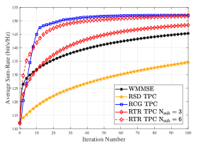
Figure 3: Convergence comparison under TPC at SNR=20dB

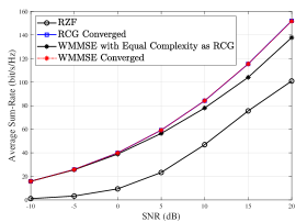
Figure 4: WSR performance when RCG method converges under TPC

V Numerical Results

In this section, we provide simulation results to demonstrate that the precoders designed in the matrix manifold framework are numerically superior and computationally efficient under different power constraints, especially when RCG method is used. We adopt the prevalent QuaDRiGa channel model [34], where ”3GPP 38.901 UMa NLOS” scenario is considered. The 25m high BS with $M_{t}=128$ antennas serves $U=20$ UTs, which are randomly distributed in the cell with radius of 250m at height of 1.5m. The antenna type is ”3gpp-3d” at the BS side and ”ula” at the user side. For simplicity, we set $M_{i}=d_{i}=2,P_{i}=\frac{P}{U},\forall i\in\mathcal{U}$. The center frequency is set at 4.8 GHz. The weighted factor of each user is set to be $1$.

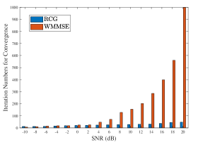
Figure 5: Convergence comparison between RCG and WMMSE under TPC

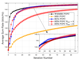
Figure 6: Convergence comparison under PUPC at SNR=20dB

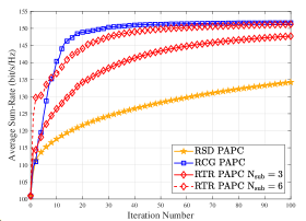
Figure 7: Convergence comparison under PAPC at SNR=20dB

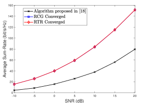
Figure 8: WSR performance when RCG method converges under PAPC

Fig. 4 depicts the convergence trajectories of the Riemannian design methods compared with WMMSE method [9] under TPC at SNR$=20$ dB for massive MIMO downlink. As shown in Fig. 4, RCG method converges much faster than RSD, WMMSE and RTR methods when $N_{\text{sub}}=3$. RTR method converges the fastest at the very beginning when $N_{\text{sub}}=6$ and obtains $87\%$ performance in the first three iterations. Besides, the complexity of RCG method is lower than that of WMMSE method. For the fairness of comparison, Fig. 4 compares the WSR performance of RCG method with that of WMMSE precoder under the same complexity when RCG method converges. As we can see, RCG method has the same performance as WMMSE method when they converge and has an evident performance gain in the high SNR regime when they share the same computational complexity. The regularized zero-forcing (RZF) method requires the least computation among these methods but also exhibits the poorest performance. To investigate the convergence behavior of RCG method, we compare the approximate iterations needed for RCG and WMMSE methods to completely converge in Fig. 6. Compared with WMMSE method, RCG method needs much fewer iterations to converge, especially when SNR is high, which clearly demonstrates the fast convergence and high computational efficiency of RCG method.

The convergence behavior of Riemannian design methods under PUPC at SNR$=20$ dB is shown in Fig. 6. When $N_{\text{sub}}=6$, RTR method needs nearly the same number of iterations to converge as RCG at the cost of a much higher computational complexity. In addition, WMMSE achieves good performance and converges fast at the first thirty iterations. However, RCG shows a better performance and converges faster compared with WMMSE when $N_{\text{out}}>30$ with a much lower computational complexity.

Fig. 8 shows the convergence behavior of Riemannian design methods under PAPC at SNR$=20$ dB. From Fig. 8, we find that RTR method converges fast in the first three iterations but RCG method converges faster when $N_{\text{out}}>10$. Fig. 8 compares the WSR performance of RCG and RTR methods when converged with the method proposed in [17]. As we can see in Fig. 8, RTR and RCG methods have the same WSR performance when converged. Compared with the algorithm proposed in [17], RCG method is numerically superior in designing precoders under PAPC with a lower computational complexity.

VI Conclusion

In this paper, we have investigated the linear precoder design methods with matrix manifold in massive MIMO downlink transmission. We focus on the WSR-maximization precoder design and demonstrate that the precoders under TPC, PUPC and PAPC are on different Riemannian submanifolds. Then the constrained problems are transformed into unconstrained ones on Riemannian submanifolds. Furthermore, RSD, RCG and RTR methods are proposed for optimizing on Riemannian submanifolds. There is no inverse of large dimensional matrix in the proposed methods. Besides, the complexity of implementing these Riemannian design methods on different Riemannian submanifolds is investigated. Simulation results show the numerical superiority and computational efficiency of RCG method.

Appendix A Proof of Theorem 1

A-A Proof for TPC case

With the fact that the Frobenius norm of $\hat{\mathbf{P}}$ is a constant, the constraint $\mathrm{tr}\left(\mathbf{P}^{H}\mathbf{P}\right)=P$ defines a sphere naturally. Clearly, $\widehat{\mathcal{M}}$ is a subset of the set $\mathbb{C}^{M_{t}\times d_{1}}\times\mathbb{C}^{M_{t}\times d_{2}}\times\cdots\times\mathbb{C}^{M_{t}\times d_{i}}$. Consider differentiable function $F_{1}:\mathcal{M}\rightarrow\mathbb{R}:\mathbf{P}\mapsto\mathrm{tr}\left(\mathbf{P}\mathbf{P}^{H}\right)-P$, and clearly $\widehat{\mathcal{M}}\in F_{1}^{-1}\left(0\right)$, where $0\in\mathbb{R}$. Based on the submersion theorem [22, Proposition 3.3.3], to show $\widehat{\mathcal{M}}$ is a closed embedded submanifold of $\mathcal{M}$, we need to prove $F_{1}$ as a submersion at each point of $\widehat{\mathcal{M}}$. In other words, we should verify that the rank of $F_{1}$ is equal to the dimension of $\mathbb{R}$, i.e., 1, at every point of $\widehat{\mathcal{M}}$. Since the rank of $F_{1}$ at a point $\mathbf{P}\in\mathcal{M}$ is defined as the dimension of the range of $\mathrm{D}F_{1}\left(\mathbf{P}\right)$, we simply need to show that for all $w\in\mathbb{R}$, there exists $\mathbf{Z}=\left(\mathbf{Z}_{1},\mathbf{Z}_{2},\cdots,\mathbf{Z}_{i}\right)\in\mathcal{M}$ such that $\mathrm{D}F_{1}\left(\mathbf{P}\right)\left[\mathbf{Z}\right]=w$. Since the differential operation at $\mathbf{P}$ is equivalent to the component-wise differential at each of $\mathbf{P}_{1},\mathbf{P}_{2},\cdots,\mathbf{P}_{i}$, we have

$$\mathrm{D}F_{1}\left(\mathbf{P}\right)\left[\mathbf{Z}\right]=\mathrm{tr}\left(\mathbf{P}^{H}\mathbf{Z}+\mathbf{Z}^{H}\mathbf{P}\right).$$ (74)

It is easy to see that if we choose $\mathbf{Z}_{i}=\frac{1}{2}\frac{w}{P}\mathbf{P}_{i}$, we will have $\mathrm{D}F_{1}\left(\mathbf{P}\right)\left[\mathbf{Z}\right]=w$. This shows that $F_{1}$ is full rank as well as a submersion on $\widehat{\mathcal{M}}$.

Because every tangent space $T_{\hat{\mathbf{P}}}\widehat{\mathcal{M}}$ is a subspace of $T_{\mathbf{P}}\mathcal{M}$, the Riemannian metric $g_{\mathbf{P}}\left(\cdot\right)$ of $\mathcal{M}$ is naturally introduced to $\widehat{\mathcal{M}}$ as $g_{\hat{\mathbf{P}}}\left(\cdot\right)=g_{\mathbf{P}}\left(\cdot\right)$. With this metric, $\widehat{\mathcal{M}}$ is an Riemannian embedded submanifold of $\mathcal{M}$.

A-B Proof for PUPC case

Note that each $\tilde{\mathbf{P}}_{i}$ in $\tilde{\mathbf{P}}$ forms a sphere. Thus $\widetilde{\mathcal{M}}$ forms an oblique manifold composed of $U$ spheres. To show $\widetilde{\mathcal{M}}$ is a Riemannian submanifold of the product manifold $\mathcal{M}$, we need to show that for $\mathbf{D}_{i}=a_{i}\mathbf{I}_{d_{i}},\forall i\in\mathcal{U}$, where $a_{i}\in\mathbb{R}$, there exists $\mathbf{Z}=\left(\mathbf{Z}_{1},\cdots,\mathbf{Z}_{U}\right)\in\mathcal{M}$ such that $\mathrm{D}F_{2}\left(\mathbf{P}\right)\left[\mathbf{Z}\right]=\mathrm{blkdiag}\left(\mathbf{D}_{1},\cdots,\mathbf{D}_{U}\right)=\mathbf{D}$. Since the differential operation at $\mathbf{P}$ is equivalent to the component-wise differential at each of $\mathbf{P}_{1},\mathbf{P}_{2},\cdots,\mathbf{P}_{U}$, we have

$$\mathrm{D}F_{2}\left(\mathbf{P}\right)\left[\mathbf{Z}\right]=$$ (75)

$$\left(\mathrm{tr}\left(\mathbf{P}_{1}^{H}\mathbf{Z}_{1}+\mathbf{Z}_{1}^{H}\mathbf{P}_{1}\right)\mathbf{I}_{d_{1}},\cdots,\mathrm{tr}\left(\mathbf{P}_{U}^{H}\mathbf{Z}_{U}+\mathbf{Z}_{U}^{H}\mathbf{P}_{U}\right)\mathbf{I}_{d_{U}}\right).$$

It is easy to see that if we choose $\mathbf{Z}_{i}=\frac{1}{2}\frac{U}{P}\mathbf{P}_{i}\mathbf{D}_{i}$, we will have $\mathrm{D}F_{2}\left(\mathbf{P}\right)\left[\mathbf{Z}\right]=\mathbf{D}$. This shows that $F_{2}$ is full rank as well as a submersion on $\widetilde{\mathcal{M}}$.

Because every tangent space $T_{\tilde{\mathbf{P}}}\widetilde{\mathcal{M}}$ is a subspace of $T_{\mathbf{P}}\mathcal{M}$, the Riemannian metric $g_{\mathbf{P}}\left(\cdot\right)$ of $\mathcal{M}$ is naturally introduced to $\widetilde{\mathcal{M}}$ as $g_{\tilde{\mathbf{P}}}\left(\cdot\right)=g_{\mathbf{P}}\left(\cdot\right)$. With this metric, $\widetilde{\mathcal{M}}$ is an Riemannian embedded submanifold of $\mathcal{M}$.

A-C Proof for PAPC case

Every column of $\bar{\mathbf{P}}^{H}$ forms a sphere and thus $\bar{\mathbf{P}}^{H}$ forms a standard oblique manifold composed of $M_{t}$ spheres. Similarly, to show $\overline{\mathcal{M}}$ is a Riemannian submanifold of the product manifold $\mathcal{M}$, we need to show that for all $\mathbf{w}=\left(w_{1},w_{2},\cdots,w_{M_{t}}\right)\in\mathbb{R}^{M_{t}}$, there exists $\mathbf{Z}=\left(\mathbf{Z}_{1},\mathbf{Z}_{2},\cdots,\mathbf{Z}_{U}\right)\in\mathcal{M}$ such that $\mathrm{D}F\left(\mathbf{P}\right)\left[\mathbf{Z}\right]=\mathrm{diag}\left(\mathbf{w}\right)$. Since the differential operation at $\mathbf{P}$ is equivalent to the component-wise differential at each of $\mathbf{P}_{1},\mathbf{P}_{2},\cdots,\mathbf{P}_{i}$, we have

$$\mathrm{D}F_{3}\left(\mathbf{P}\right)\left[\mathbf{Z}\right]=\mathbf{I}_{M_{t}}\odot\sum_{i=1}^{U}\left(\mathbf{P}_{i}\mathbf{Z}_{i}^{H}+\mathbf{Z}_{i}\mathbf{P}_{i}^{H}\right).$$ (76)

It is easy to see that if we choose $\mathbf{Z}_{i}=\frac{1}{2}\frac{M_{t}}{P}\mathrm{diag}\left(\mathbf{w}\right)\mathbf{P}_{i}$, we will have $\mathrm{D}F_{3}\left(\mathbf{P}\right)\left[\mathbf{Z}\right]=\mathrm{diag}\left(\mathbf{w}\right)$. This shows that $F_{3}$ is full rank as well as a submersion on $\overline{\mathcal{M}}$.

Because every tangent space $T_{\bar{\mathbf{P}}}\overline{\mathcal{M}}$ is a subspace of $T_{\mathbf{P}}\mathcal{M}$, the Riemannian metric $g_{\mathbf{P}}\left(\cdot\right)$ of $\mathcal{M}$ is naturally introduced to $\overline{\mathcal{M}}$ as $g_{\bar{\mathbf{P}}}\left(\cdot\right)=g_{\mathbf{P}}\left(\cdot\right)$. With this metric, $\overline{\mathcal{M}}$ is a Riemannian embedded submanifold of $\mathcal{M}$.

Appendix B Proof of Lemma 1

From the decomposition (24) and the definition of the normal space (26), it is easy to have $\Pi_{T_{\hat{\mathbf{P}}}\widehat{\mathcal{M}}}^{T_{\mathbf{P}}\mathcal{M}}\left({\boldsymbol{\xi}}_{\mathbf{P}}\right)={\boldsymbol{\xi}}_{\mathbf{P}}-\hat{\lambda}_{1}\mathbf{P}$. Meanwhile, from the definition of the tangent space (25), ${\boldsymbol{\xi}}_{\mathbf{P}}-\hat{\lambda}_{1}\mathbf{P}$ should satisfy the equation

$$\mathrm{tr}\left(\mathbf{P}^{H}\left({\boldsymbol{\xi}}_{\mathbf{P}}-\hat{\lambda}_{1}\mathbf{P}\right)+\left({\boldsymbol{\xi}}_{\mathbf{P}}-\hat{\lambda}_{1}\mathbf{P}\right)^{H}\mathbf{P}\right)=0.$$ (77)

After some algebra, we can get $\hat{\lambda}_{1}=\frac{1}{P}\Re\left\{\mathrm{tr}\left(\mathbf{P}^{H}{\boldsymbol{\xi}}_{\mathbf{P}}\right)\right\}$.

Appendix C Proof of Theorem 2

C-A Proof for Riemannian gradient in Theorem 2

To simplify the notations, we use $f\left(\mathbf{P}_{i}\right)$ to represent $f\left(\mathbf{P}\right)$ that only considers $\mathbf{P}_{i}$ as variable with $\mathbf{P}_{\ell}$ for $\ell\neq i$ fixed.

For any ${\boldsymbol{\xi}}_{\mathbf{P}_{i}}\in T_{\mathbf{P}_{i}}\mathbb{C}^{M_{t}\times M_{i}}$, the directional derivative of $f\left(\mathbf{P}_{i}\right)$ along ${\boldsymbol{\xi}}_{\mathbf{P}_{i}}$ is

$$\mathrm{D}f\left(\mathbf{P}_{i}\right)\left[{\boldsymbol{\xi}}_{\mathbf{P}_{i}}\right]=-w_{i}\mathrm{D}\mathcal{R}_{i}\left[{\boldsymbol{\xi}}_{\mathbf{P}_{i}}\right]-\sum_{\ell\neq i}^{U}w_{\ell}\mathrm{D}\mathcal{R}_{\ell}\left[{\boldsymbol{\xi}}_{\mathbf{P}_{i}}\right].$$ (78)

We derive $\mathrm{D}\mathcal{R}_{i}\left[{\boldsymbol{\xi}}_{\mathbf{P}_{i}}\right]$ and $\mathrm{D}\mathcal{R}_{\ell}\left[{\boldsymbol{\xi}}_{\mathbf{P}_{i}}\right]$ separately as

$$\mathrm{D}\mathcal{R}_{i}\left[{\boldsymbol{\xi}}_{\mathbf{P}_{i}}\right]= \mathrm{tr}\left(\mathbf{C}_{i}\left({\boldsymbol{\xi}}_{\mathbf{P}_{i}}^{H}\mathbf{H}_{i}^{H}\mathbf{A}_{i}+\mathbf{A}_{i}^{H}\mathbf{H}_{i}{\boldsymbol{\xi}}_{\mathbf{P}_{i}}\right)\right),$$ (79)

$$\mathrm{D}\mathcal{R}_{\ell}\left[{\boldsymbol{\xi}}_{\mathbf{P}_{i}}\right]= -\mathrm{tr}\bigg{(}\mathbf{H}_{\ell}^{H}\mathbf{B}_{\ell}\mathbf{H}_{\ell}\left({\boldsymbol{\xi}}_{\mathbf{P}_{i}}\mathbf{P}_{i}^{H}+\mathbf{P}_{i}{\boldsymbol{\xi}}_{\mathbf{P}_{i}}^{H}\right)\bigg{)}.$$ (80)

Thus, we have

$$\mathrm{D} f\left(\mathbf{P}_{i}\right)\left[{\boldsymbol{\xi}}_{\mathbf{P}_{i}}\right]=$$ (81)

$$g_{\mathbf{P}_{i}}\left(-2w_{i}\mathbf{H}_{i}^{H}\mathbf{A}_{i}\mathbf{C}_{i}+2\sum_{\ell\neq i}w_{\ell}\mathbf{H}_{\ell}^{H}\mathbf{B}_{\ell}\mathbf{H}_{\ell}\mathbf{P}_{i},{\boldsymbol{\xi}}_{\mathbf{P}_{i}}\right)$$

and $\mathrm{grad}f\left(\mathbf{P}_{i}\right)$ is

$$\mathrm{grad}f\left(\mathbf{P}_{i}\right)=-2\left(w_{i}\mathbf{H}_{i}^{H}\mathbf{A}_{i}\mathbf{C}_{i}-\sum_{\ell\neq i}w_{\ell}\mathbf{H}_{\ell}^{H}\mathbf{B}_{\ell}\mathbf{H}_{\ell}\mathbf{P}_{i}\right).$$ (82)

From [22, Section 3.6.1], the Riemannian gradient of $f\left(\hat{\mathbf{P}}\right)$ is

$$\mathrm{grad}f\left(\hat{\mathbf{P}}\right)=\Pi_{T_{\hat{\mathbf{P}}}\widehat{\mathcal{M}}}^{T_{\mathbf{P}}\mathcal{M}}\left(\mathrm{grad}f\left(\hat{\mathbf{P}}\right)\right)=\mathrm{grad}f\left(\mathbf{P}\right)-\hat{\lambda}_{1}\mathbf{P},$$ (83)

where $\hat{\lambda}_{1}=\frac{1}{P}\Re\left\{\mathrm{tr}\left(\mathbf{P}\left(\mathrm{grad}f\left(\mathbf{P}\right)\right)^{H}\right)\right\}$.

C-B Proof for Riemannian Hessian in Theorem 2

Combine (9) and (4), we get

$$\mathrm{Hess}f(\hat{\mathbf{P}})[{\boldsymbol{\xi}}_{\hat{\mathbf{P}}}] =\nabla_{{\boldsymbol{\xi}}_{\hat{\mathbf{P}}}}^{\widehat{\mathcal{M}}}\mathrm{grad}f$$ (84)

$$=\Pi_{T_{\hat{\mathbf{P}}}\widehat{\mathcal{M}}}^{T_{\mathbf{P}}\mathcal{M}}\left(\nabla_{{\boldsymbol{\xi}}_{\hat{\mathbf{P}}}}^{\mathcal{M}}\mathrm{grad}f\right)$$

$$=\Pi_{T_{\hat{\mathbf{P}}}\widehat{\mathcal{M}}}^{T_{\mathbf{P}}\mathcal{M}}\left(\mathrm{Dgrad}f(\hat{\mathbf{P}})[{\boldsymbol{\xi}}_{\hat{\mathbf{P}}}]\right),$$

which belongs to $T_{\hat{\mathbf{P}}}\widehat{\mathcal{M}}$. So the following relationship holds:

$$\Re\left\{\mathrm{tr}\left(\mathbf{P}^{H}\mathrm{Dgrad}f(\hat{\mathbf{P}})[{\boldsymbol{\xi}}_{\hat{\mathbf{P}}}]-\hat{\lambda}_{2}\mathbf{P}_{\ell}\right)\right\}=0$$ (85)

$$\Rightarrow\hat{\lambda}_{2}=\frac{1}{P}\Re\left\{\mathrm{tr}\left(\mathbf{P}^{H}\mathrm{Dgrad}f(\hat{\mathbf{P}})[{\boldsymbol{\xi}}_{\hat{\mathbf{P}}}]\right)\right\}.$$

Recall that $\mathrm{Hess}f(\hat{\mathbf{P}})[{\boldsymbol{\xi}}_{\hat{\mathbf{P}}}]$ is an element in $T_{\hat{\mathbf{P}}}{\widehat{\mathcal{M}}}$. Thus from (20), we can get

$$\mathrm{Hess}f(\hat{\mathbf{P}})[{\boldsymbol{\xi}}_{\hat{\mathbf{P}}}]=\left(\mathrm{Hess}f(\hat{\mathbf{P}}_{1})[{\boldsymbol{\xi}}_{\hat{\mathbf{P}}_{1}}],\cdots,\mathrm{Hess}f(\hat{\mathbf{P}}_{U})[{\boldsymbol{\xi}}_{\hat{\mathbf{P}}_{U}}]\right),$$ (86)

where $\mathrm{Hess}f(\hat{\mathbf{P}}_{i})[{\boldsymbol{\xi}}_{\hat{\mathbf{P}}_{i}}]$ can be denoted as

$$\mathrm{Hess}f(\hat{\mathbf{P}}_{i})[{\boldsymbol{\xi}}_{\hat{\mathbf{P}}_{i}}]= \mathrm{Dgrad}f(\mathbf{P}_{i})[{\boldsymbol{\xi}}_{\mathbf{P}_{i}}]$$ (87)

$$-\mathrm{D}\hat{\lambda}_{1}[{\boldsymbol{\xi}}_{\mathbf{P}_{i}}]\mathbf{P}_{i}-\hat{\lambda}_{1}{\boldsymbol{\xi}}_{\mathbf{P}_{i}}-\hat{\lambda}_{2}\mathbf{P}_{i}.$$

$\mathrm{Dgrad}f(\mathbf{P}_{i})[{\boldsymbol{\xi}}_{\mathbf{P}_{i}}]$ and $\mathrm{D}\hat{\lambda}_{1}[{\boldsymbol{\xi}}_{\mathbf{P}_{i}}]$ remain unknown. For notational simplicity, let us define

$$\mathbf{M}_{\ell,i}=\mathbf{H}_{\ell}{\boldsymbol{\xi}}_{\mathbf{P}_{i}}\mathbf{P}_{i}^{H}\mathbf{H}_{\ell}^{H}+\mathbf{H}_{\ell}\mathbf{P}_{i}{\boldsymbol{\xi}}_{\mathbf{P}_{i}}^{H}\mathbf{H}_{\ell}^{H},$$ (88)

$$\mathbf{F}_{\ell,i}=-\mathbf{R}_{\ell}^{-1}\mathbf{M}_{\ell,i}\mathbf{B}_{\ell},\ \mathbf{E}_{\ell,i}=-\mathbf{B}_{\ell}\mathbf{M}_{\ell,i}\mathbf{B}_{\ell},$$

then we can get

$$\mathrm{D}\mathbf{B}_{\ell}\left[{\boldsymbol{\xi}}_{\mathbf{P}_{i}}\right] =\mathbf{F}_{\ell,i}+\mathbf{F}_{\ell,i}^{H}+\mathbf{E}_{\ell,i}.$$ (89)

Then $\mathrm{Dgrad}f(\mathbf{P}_{i})[{\boldsymbol{\xi}}_{\mathbf{P}_{i}}]$ can be calculated as follows:

$$\mathrm{Dgrad}f(\mathbf{P}_{i})[{\boldsymbol{\xi}}_{\mathbf{P}_{i}}]=-2w_{i}\mathbf{H}_{i}^{H}\mathbf{R}_{i}^{-1}\mathbf{H}_{i}{\boldsymbol{\xi}}_{\mathbf{P}_{i}}\mathbf{C}_{i}$$ (90)

$$+2w_{i}\mathbf{H}_{i}^{H}\mathbf{A}_{i}\mathbf{C}_{i}\left({\boldsymbol{\xi}}_{\mathbf{P}_{i}}^{H}\mathbf{H}_{i}^{H}\mathbf{A}_{i}+\mathbf{A}_{i}^{H}\mathbf{H}_{i}{\boldsymbol{\xi}}_{\mathbf{P}_{i}}\right)\mathbf{C}_{i}$$

$$+2\sum_{\ell\neq i}w_{\ell}\mathbf{H}_{\ell}^{H}\mathbf{B}_{\ell}\mathbf{H}_{\ell}{\boldsymbol{\xi}}_{\mathbf{P}_{i}}+2\sum_{\ell\neq i}w_{\ell}\mathbf{H}_{\ell}^{H}\mathrm{D}\mathbf{B}_{\ell}\left[{\boldsymbol{\xi}}_{\mathbf{P}_{i}}\right]\mathbf{H}_{\ell}\mathbf{P}_{i}.$$

$\mathrm{D}\hat{\lambda}_{1}[{\boldsymbol{\xi}}_{\mathbf{P}_{i}}]$ can be calculated as follows:

$$\mathrm{D}\hat{\lambda}_{1}[{\boldsymbol{\xi}}_{\mathbf{P}_{i}}]=$$ (91)

$$\frac{1}{P}\Re\left\{\mathrm{tr}\left({\boldsymbol{\xi}}_{\mathbf{P}_{i}}^{H}\mathrm{grad}f(\mathbf{P}_{i})+\mathbf{P}_{i}^{H}\mathrm{Dgrad}f(\mathbf{P}_{i})[{\boldsymbol{\xi}}_{\mathbf{P}_{i}}]\right)\right\}.$$

Appendix D Proof of Riemannian Hessian in Theorem 3

Like (84), we get

$$\mathrm{Hess}f(\tilde{\mathbf{P}})[{\boldsymbol{\xi}}_{\tilde{\mathbf{P}}}]=\Pi_{T_{\tilde{\mathbf{P}}}\widetilde{\mathcal{M}}}^{T_{\mathbf{P}}\mathcal{M}}\left(\mathrm{Dgrad}f(\tilde{\mathbf{P}})[{\boldsymbol{\xi}}_{\tilde{\mathbf{P}}}]\right),$$ (92)

which belongs to $T_{\tilde{\mathbf{P}}}\widetilde{\mathcal{M}}$, so the following relationship holds:

$$\Re\left\{\mathrm{tr}\left(\tilde{\mathbf{P}}_{i}^{H}\left(\mathrm{Dgrad}f(\tilde{\mathbf{P}}_{i})[{\boldsymbol{\xi}}_{\tilde{\mathbf{P}}_{i}}]-\tilde{\mathbf{P}}_{i}\left[\tilde{{\boldsymbol{\Lambda}}}_{2}\right]_{i}\right)\right)\right\}=0$$ (93)

$$\Rightarrow\left[\tilde{{\boldsymbol{\Lambda}}}_{2}\right]_{i}=\Re\left\{\mathrm{tr}\left(\mathbf{P}_{i}^{H}\left(\mathrm{Dgrad}f(\tilde{\mathbf{P}}_{i})[{\boldsymbol{\xi}}_{\tilde{\mathbf{P}}_{i}}]\right)\right)\right\}\mathbf{I}_{d_{i}}.$$

From (20), we can get

$$\mathrm{Hess}f(\tilde{\mathbf{P}})[{\boldsymbol{\xi}}_{\tilde{\mathbf{P}}}]= \left(\mathrm{Hess}f(\tilde{\mathbf{P}}_{1})[{\boldsymbol{\xi}}_{\tilde{\mathbf{P}}_{1}}],\cdots,\mathrm{Hess}f(\tilde{\mathbf{P}}_{U})[{\boldsymbol{\xi}}_{\tilde{\mathbf{P}}_{U}}]\right),$$ (94)

where

$$\mathrm{Hess}f(\tilde{\mathbf{P}}_{i})[{\boldsymbol{\xi}}_{\tilde{\mathbf{P}}_{i}}]=\mathrm{Dgrad}f(\mathbf{P}_{i})[{\boldsymbol{\xi}}_{\mathbf{P}_{i}}]$$ (95)

$$-\mathbf{P}_{i}\mathrm{D}\left[\tilde{{\boldsymbol{\Lambda}}}_{1}\right]_{i}[{\boldsymbol{\xi}}_{\mathbf{P}_{i}}]-{\boldsymbol{\xi}}_{\mathbf{P}_{i}}\left[\tilde{{\boldsymbol{\Lambda}}}_{1}\right]_{i}-\mathbf{P}_{i}\left[\tilde{{\boldsymbol{\Lambda}}}_{2}\right]_{i}.$$

$\mathrm{D}\left[\tilde{{\boldsymbol{\Lambda}}}_{1}\right]_{i}[{\boldsymbol{\xi}}_{\mathbf{P}_{i}}]$ remains unknown, which can be calculated as follows:

$$\mathrm{D}\left[\tilde{{\boldsymbol{\Lambda}}}_{1}\right]_{i}[{\boldsymbol{\xi}}_{\mathbf{P}_{i}}]=$$ (96)

$$\frac{1}{P_{i}}\Re\left\{\mathrm{tr}\left({\boldsymbol{\xi}}_{\mathbf{P}_{i}}^{H}\mathrm{grad}f(\mathbf{P}_{i})+\mathbf{P}_{i}^{H}\mathrm{Dgrad}f(\mathbf{P}_{i})[{\boldsymbol{\xi}}_{\mathbf{P}_{i}}]\right)\right\}\mathbf{I}_{d_{i}},$$

where $\mathrm{Dgrad}f\left(\mathbf{P}_{i}\right)\left[{\boldsymbol{\xi}}_{\mathbf{P}_{i}}\right]$ has been calculated in Appendix C-B.

Appendix E Proof of Riemannian Hessian in Theorem 4

Like (84), we get

$$\mathrm{Hess}f(\bar{\mathbf{P}})[{\boldsymbol{\xi}}_{\bar{\mathbf{P}}}]=\Pi_{T_{\bar{\mathbf{P}}}\overline{\mathcal{M}}}^{T_{\mathbf{P}}\mathcal{M}}\left(\mathrm{Dgrad}f(\bar{\mathbf{P}})[{\boldsymbol{\xi}}_{\bar{\mathbf{P}}}]\right),$$ (97)

which belongs to $T_{\bar{\mathbf{P}}}\overline{\mathcal{M}}$, so the following relationship holds:

$$\mathbf{I}_{M_{t}}\odot\sum_{l=1}^{K}\Re\left\{\bar{\mathbf{P}}_{\ell}\left(\mathrm{Dgrad}f(\bar{\mathbf{P}})[{\boldsymbol{\xi}}_{\bar{\mathbf{P}}}]-\bar{{\boldsymbol{\Lambda}}}_{2}\mathbf{P}_{\ell}\right)^{H}\right\}=0$$ (98)

$$\Rightarrow\bar{{\boldsymbol{\Lambda}}}_{2}=\frac{M_{t}}{P}\mathbf{I}_{M_{t}}\odot\sum_{l=1}^{K}\Re\left\{\mathbf{P}_{\ell}\left(\mathrm{Dgrad}f(\bar{\mathbf{P}})[{\boldsymbol{\xi}}_{\bar{\mathbf{P}}}]\right)^{H}\right\}.$$

From (20), we can get

$$\mathrm{Hess}f(\bar{\mathbf{P}})[{\boldsymbol{\xi}}_{\bar{\mathbf{P}}}]=\left(\mathrm{Hess}f(\bar{\mathbf{P}}_{1})[{\boldsymbol{\xi}}_{\bar{\mathbf{P}}_{1}}],\cdots,\mathrm{Hess}f(\bar{\mathbf{P}}_{U})[{\boldsymbol{\xi}}_{\bar{\mathbf{P}}_{U}}]\right),$$ (99)

where $\mathrm{Hess}f(\bar{\mathbf{P}}_{i})[{\boldsymbol{\xi}}_{\bar{\mathbf{P}}_{i}}]$ can be denoted as:

$$\mathrm{Hess}f(\bar{\mathbf{P}}_{i})[{\boldsymbol{\xi}}_{\bar{\mathbf{P}}_{i}}]=$$ (100)

$$\mathrm{Dgrad}f(\mathbf{P}_{i})[{\boldsymbol{\xi}}_{\mathbf{P}_{i}}]-\mathrm{D}\bar{{\boldsymbol{\Lambda}}}_{1}[{\boldsymbol{\xi}}_{\mathbf{P}_{i}}]\mathbf{P}_{i}-\bar{{\boldsymbol{\Lambda}}}_{1}{\boldsymbol{\xi}}_{\mathbf{P}_{i}}-\bar{{\boldsymbol{\Lambda}}}_{2}\mathbf{P}_{i}.$$

$\mathrm{Dgrad}f\left(\mathbf{P}_{i}\right)\left[{\boldsymbol{\xi}}_{\mathbf{P}_{i}}\right]$ has been calculated in Appendix C-B. $\mathrm{D}\bar{{\boldsymbol{\Lambda}}}_{1}[{\boldsymbol{\xi}}_{\mathbf{P}_{i}}]$ remains unknown, which can be calculated as follows:

$$\mathrm{D}\bar{{\boldsymbol{\Lambda}}}_{1}[{\boldsymbol{\xi}}_{\mathbf{P}_{i}}]=\frac{M_{t}}{P}\mathbf{I}_{M_{t}}\odot\Re\sum_{l\neq i}\left\{\mathbf{P}_{\ell}\left(\mathrm{Dgrad}f\left(\mathbf{P}_{\ell}\right)\left[{\boldsymbol{\xi}}_{\mathbf{P}_{i}}\right]\right)^{H}\right\}+$$ (101)

$$\frac{M_{t}}{P}\mathbf{I}_{M_{t}}\odot\Re\left\{{\boldsymbol{\xi}}_{\mathbf{P}_{i}}\left(\mathrm{grad}f(\mathbf{P}_{i})\right)^{H}+\mathbf{P}_{i}\mathrm{Dgrad}f(\mathbf{P}_{i})[{\boldsymbol{\xi}}_{\mathbf{P}_{i}}]^{H}\right\}.$$

$\mathrm{Dgrad}f\left(\mathbf{P}_{\ell}\right)\left[{\boldsymbol{\xi}}_{\mathbf{P}_{i}}\right]$ for $\forall\ell\neq i$ remains to be calculated:

$$\mathrm{Dgrad}f\left(\mathbf{P}_{\ell}\right)=2\sum_{j\neq\ell}w_{j}\mathbf{H}_{j}^{H}\mathrm{D}\mathbf{B}_{j}\left[{\boldsymbol{\xi}}_{\mathbf{P}_{i}}\right]\mathbf{H}_{j}\mathbf{P}_{\ell}\left[{\boldsymbol{\xi}}_{\mathbf{P}_{i}}\right]$$ (102)

$$+2w_{\ell}\mathbf{H}_{\ell}^{H}\mathbf{R}_{\ell}^{-1}\mathbf{M}_{\ell,i}\mathbf{A}_{\ell}\mathbf{C}_{\ell}-2w_{\ell}\mathbf{H}_{\ell}^{H}\mathbf{A}_{\ell}\mathrm{D}\mathbf{C}_{\ell}\left[{\boldsymbol{\xi}}_{\mathbf{P}_{i}}\right],$$

where

$$\mathrm{D}\mathbf{C}_{\ell}\left[{\boldsymbol{\xi}}_{\mathbf{P}_{i}}\right]= -\mathbf{C}_{\ell}\mathbf{A}_{\ell}^{H}\mathbf{M}_{\ell,i}\mathbf{A}_{\ell}\mathbf{C}_{\ell},\forall\ell\neq i,$$ (103a)

$$\mathrm{D}\mathbf{B}_{j}\left[{\boldsymbol{\xi}}_{\mathbf{P}_{i}}\right]= \begin{cases}\mathbf{F}_{j,i}+\mathbf{F}_{j,i}^{H}+\mathbf{E}_{j,i},j\neq\ell\&j\neq i,\\ \mathbf{R}_{i}^{-1}\mathbf{H}_{i}\left({\boldsymbol{\xi}}_{\mathbf{P}_{i}}\mathbf{C}_{i}\mathbf{P}_{i}^{H}+\mathbf{P}_{i}\mathbf{C}_{i}{\boldsymbol{\xi}}_{\mathbf{P}_{i}}^{H}\right)*\\ \mathbf{H}_{i}^{H}\mathbf{R}_{i}^{-1}+\mathbf{E}_{i,i},j=i.\end{cases}$$ (103b)

References

- [1] E. Björnson, L. Sanguinetti, H. Wymeersch, J. Hoydis, and T. L. Marzetta, “Massive MIMO is a reality—What is next?: Five promising research directions for antenna arrays,” Digit. Signal Process., vol. 94, pp. 3–20, Nov. 2019.
- [2] E. D. Carvalho, A. Ali, A. Amiri, M. Angjelichinoski, and R. W. Heath, “Non-stationarities in extra-large-scale massive MIMO,” IEEE Wireless Commun., vol. 27, pp. 74–80, Aug. 2020.
- [3] T. L. Marzetta and H. Yang, Fundamentals of Massive MIMO. Cambridge University Press, 2016.
- [4] E. G. Larsson, O. Edfors, F. Tufvesson, and T. L. Marzetta, “Massive MIMO for next generation wireless systems.” IEEE Commun. Mag., vol. 52, no. 2, pp. 186–195, Feb. 2014.
- [5] T. Ketseoglou, M. C. Valenti, and E. Ayanoglu, “Millimeter wave massive MIMO downlink per-group communications with hybrid linear precoding,” IEEE Trans. Veh. Technol., vol. 70, no. 7, pp. 6841–6854, Jul. 2021.
- [6] S. Jing and C. Xiao, “Linear MIMO precoders with finite alphabet inputs via stochastic optimization and deep neural networks (DNNs),” IEEE Trans. Signal Process., vol. 69, pp. 4269–4281, 2021.
- [7] Y. Zhang, P. Mitran, and C. Rosenberg, “Joint resource allocation for linear precoding in downlink massive MIMO systems,” IEEE Trans. Commun., vol. 69, no. 5, pp. 3039–3053, May 2021.
- [8] V. M. T. Palhares, A. R. Flores, and R. C. de Lamare, “Robust MMSE precoding and power allocation for cell-free massive MIMO systems,” IEEE Trans. Veh. Technol., vol. 70, no. 5, pp. 5115–5120, May 2021.
- [9] S. S. Christensen, R. Agarwal, E. De Carvalho, and J. M. Cioffi, “Weighted sum-rate maximization using weighted MMSE for MIMO-BC beamforming design,” IEEE Trans. Wireless Commun., vol. 7, no. 12, pp. 4792–4799, Dec. 2008.
- [10] T. X. Vu, S. Chatzinotas, and B. Ottersten, “Dynamic bandwidth allocation and precoding design for highly-loaded multiuser MISO in beyond 5G networks,” IEEE Trans. Wireless Commun., vol. 21, no. 3, pp. 1794–1805, Mar. 2022.
- [11] J. Zhang, C.-K. Wen, C. Yuen, S. Jin, and X. Q. Gao, “Large system analysis of cognitive radio network via partially-projected regularized zero-forcing precoding,” IEEE Trans. Wireless Commun., vol. 14, no. 9, pp. 4934–4947, Sep. 2015.
- [12] T. X. Tran and K. C. Teh, “Spectral and energy efficiency analysis for SLNR precoding in massive MIMO systems with imperfect CSI,” IEEE Trans. on Wireless Commun., vol. 17, no. 6, pp. 4017–4027, Jun. 2018.
- [13] L. You, X. Qiang, K.-X. Li, C. G. Tsinos, W. Wang, X. Q. Gao, and B. Ottersten, “Massive MIMO hybrid precoding for LEO satellite communications with twin-resolution phase shifters and nonlinear power amplifiers,” IEEE Trans. Commun., vol. 70, no. 8, pp. 5543–5557, Aug. 2022.
- [14] A.-A. Lu, X. Q. Gao, W. Zhong, C. Xiao, and X. Meng, “Robust transmission for massive MIMO downlink with imperfect CSI,” IEEE Trans. Commun., vol. 67, no. 8, pp. 5362–5376, Aug. 2019.
- [15] R. Muharar, R. Zakhour, and J. Evans, “Optimal power allocation and user loading for multiuser MISO channels with regularized channel inversion,” IEEE Trans. Commun., vol. 61, no. 12, pp. 5030–5041, Dec. 2013.
- [16] M. Mazrouei-Sebdani and W. A. Krzymień, “On MMSE vector-perturbation precoding for MIMO broadcast channels with per-antenna-group power constraints,” IEEE Trans. Signal Process., vol. 61, no. 15, pp. 3745–3751, Aug. 2013.
- [17] J. Choi, S. Han, and J. Joung, “Low-complexity multiuser MIMO precoder design under per-antenna power constraints,” IEEE Trans. Veh. Technol., vol. 67, no. 9, pp. 9011–9015, Sep. 2018.
- [18] J. Chen, Y. Yin, T. Birdal, B. Chen, L. J. Guibas, and H. Wang, “Projective manifold gradient layer for deep rotation regression,” Proc. IEEE Conf. Comput. Vis. Pattern Recog., pp. 6646–6655, 2022.
- [19] K. Li and R. Chen, “Batched data-driven evolutionary multiobjective optimization based on manifold interpolation,” IEEE Trans. Evol. Comput., vol. 27, no. 1, pp. 126–140, Feb. 2023.
- [20] C. Feres and Z. Ding, “A riemannian geometric approach to blind signal recovery for grant-free radio network access,” IEEE Trans. Signal Process., vol. 70, pp. 1734–1748, 2022.
- [21] J. Dong, K. Yang, and Y. Shi, “Blind demixing for low-latency communication,” IEEE Trans. Wireless Commun., vol. 18, no. 2, pp. 897–911, Feb. 2019.
- [22] P.-A. Absil, R. Mahony, and R. Sepulchre, Optimization Algorithms on Matrix Manifolds. Princeton, NJ, USA: Princeton Univ. Press, 2009.
- [23] N. Boumal, An Introduction to Optimization on Smooth Manifolds. Cambridge University Press, 2023.
- [24] J. M. Lee and J. M. Lee, Smooth Manifolds. Springer, 2012.
- [25] R. Abraham, J. E. Marsden, and T. Ratiu, Manifolds, Tensor Analysis, and Applications. Springer Science & Business Media, 2012, vol. 75.
- [26] W. Guo, A.-A. Lu, X. Meng, X. Q. Gao, and N. Ma, “Broad coverage precoding design for massive MIMO with manifold optimization,” IEEE Trans. Commun., vol. 67, no. 4, pp. 2792–2806, Apr. 2019.
- [27] P.-A. Absil and K. Gallivan, “Joint diagonalization on the oblique manifold for independent component analysis,” in Proc. IEEE Int. Conf. Acoust. Speech Signal Process., 2006, pp. 945–948.
- [28] C. Wang, A.-A. Lu, X. Q. Gao, and Z. Ding, “Robust precoding for 3D massive MIMO configuration with matrix manifold optimization,” IEEE Trans. Wireless Commun., vol. 21, no. 5, pp. 3423–3437, May 2022.
- [29] J. Li, G. Liao, Y. Huang, Z. Zhang, and A. Nehorai, “Riemannian geometric optimization methods for joint design of transmit sequence and receive filter on MIMO radar,” IEEE Trans. Signal Process., vol. 68, pp. 5602–5616, 2020.
- [30] J. Sun, Q. Qu, and J. Wright, “Complete dictionary recovery over the sphere ii: Recovery by riemannian trust-region method,” IEEE Trans. on Inf. Theory, vol. 63, no. 2, pp. 885–914, Feb. 2017.
- [31] A. R. Conn, N. I. M. Gould, and P. L. Toint, Trust Region Methods. Philadelphia: SIAM, 2000, vol. 1.
- [32] P.-A. Absil, C. G. Baker, and K. A. Gallivan, “Trust-region methods on riemannian manifolds.” Found. Comput. Math., vol. 7, no. 3, pp. 303–330, Jul. 2007.
- [33] Q. Shi, M. Razaviyayn, Z.-Q. Luo, and C. He, “An iteratively weighted MMSE approach to distributed sum-utility maximization for a MIMO interfering broadcast channel,” IEEE Trans. Signal Process., vol. 59, no. 9, pp. 4331–4340, Sep. 2011.
- [34] S. Jaeckel, L. Raschkowski, K. Borner, and L. Thiele, “Quadriga: A 3-D multi-cell channel model with time evolution for enabling virtual field trials,” IEEE Trans. Antennas Propag., vol. 62, no. 6, pp. 3242–3256, Jun. 2014.