Diffusion map particle systems for generative modeling

Abstract.

We propose a novel diffusion map particle system (DMPS) for generative modeling, based on diffusion maps and Laplacian-adjusted Wasserstein gradient descent (LAWGD). Diffusion maps are used to approximate the generator of the corresponding Langevin diffusion process from samples, and hence to learn the underlying data-generating manifold. On the other hand, LAWGD enables efficient sampling from the target distribution given a suitable choice of kernel, which we construct here via a spectral approximation of the generator, computed with diffusion maps. Our method requires no offline training and minimal tuning, and can outperform other approaches on data sets of moderate dimension.

1. Introduction

Generative modeling is a central task in fields such as computer vision (Cai et al., 2020; Ho et al., 2021; Rombach et al., 2021; Shaham et al., 2019; Yeh et al., 2017; Ranzato et al., 2011) and natural language processing (Yogatama et al., 2017; Miao and Blunsom, 2016; Li et al., 2018, 2022), and applications ranging from medical image analysis (Yi et al., 2019; Nie et al., 2017; Kazeminia et al., 2020; Mahapatra et al., 2019) to protein design (Anand and Huang, 2018; Wu et al., 2021). Despite their successes, popular generative models such as variational auto-encoders (VAE) (Kingma and Welling, 2013; Rezende et al., 2014), generative adversarial networks (GAN) (Goodfellow et al., 2014), and diffusion models or score-based generative models (SGM) (Ho et al., 2020; Song and Ermon, 2019; Song et al., 2020; Yang et al., 2022), typically need careful hyperparameter tuning (Ruthotto and Haber, 2021; Song and Ermon, 2020) and may involve long convergence times, e.g., for Langevin-type sampling (Franzese et al., 2022). The performance of such methods highly depends on the architecture and the choice of parameters of deep neural networks (Salimans et al., 2016; Khandelwal and Krishnan, 2019), which, all too often, require expert knowledge.

In this paper, we propose a new nonparametric kernel-based approach to generative modeling, based on diffusion maps and interacting particle systems.

Diffusion maps (Coifman et al., 2005; Coifman and Lafon, 2006; Nadler et al., 2005, 2006), along with many other graph-based methods (Belkin and Niyogi, 2003; Tenenbaum et al., 2011; Roweis and Saul, 2000), have mainly been used as a tool for nonlinear dimension reduction. The kernel matrix, constructed using pairwise distances between samples with proper normalization, approximates the generator of a Langevin diffusion process. This approximation becomes exact as the number of samples goes to infinity and the kernel bandwidth goes to zero. Construction of the kernel matrix using smooth kernels (e.g., Gaussians) enables one to compute the inverse of the eigenvalues and the gradients of the eigenfunctions analytically.

Separately, the notion of gradient flow (Santambrogio, 2016; Ambrosio et al., 2005; Daneri and Savaré, 2010) underlies a very active field of research and offers a unifying perspective on sampling and optimization (Jordan et al., 1998; Wibisono, 2018), with numerous connections to partial differential equations and differential geometry (Villani, 2008; Adams et al., 2013). Many common sampling algorithms approximate the gradient flow (of some functional) on a space of probability measures. The unadjusted Langevin algorithm (ULA) is a canonical example, and follows from the time discretization of a Langevin SDE. But many other particle systems, particularly interacting particle systems, approximate gradient flows: examples include Stein variational gradient descent (SVGD) (Liu, 2017; Liu and Wang, 2016), affine-invariant interacting Langevin dynamics (ALDI) (Garbuno-Iñigo et al., 2019), and Laplacian-adjusted Wasserstein gradient descent (LAWGD) (Chewi et al., 2020). ULA, SVGD, and other algorithms access the target distribution via the gradient of its log-density, and hence many of these methods have become popular for Bayesian inference.

Our approach combines these two ideas by using diffusion maps to directly approximate (the gradient of the inverse of) the generator of the Langevin diffusion process from samples, and in turn using this approximation within LAWGD to produce more samples efficiently. Compared to other generative modeling methods, our approach has several advantages. First, the use of diffusion maps facilitates accurate sampling from distributions supported on manifolds, particularly when the dimension of the manifold is lower than that of the ambient space. Second, we demonstrate accurate sampling from distributions with (a priori unknown) bounded support. Both of these features are in contrast with methods driven only by approximations of the local score: we conjecture that such methods are less able to detect the overall geometry of the target distribution, whereas our approach harnesses graph-based methods that are widely used for nonlinear dimension reduction to approximate the generator as a whole. Finally, our method is quite simple and computationally efficient comparing to training a neural network (e.g., as in score-based generative modeling) (Song and Ermon, 2019) or normalizing flows (Caterini et al., 2021; Ho et al., 2019): the only parameter that needs to be tuned is the kernel bandwidth, and no offline training is required.

2. Notation and preliminaries

We use $\pi$ to denote the underlying target distribution, i.e., the distribution we would like to sample from, and let $V$ denote the potential, where $\pi\propto\exp(-V)$. Let $\mathcal{P}_{2}(\mathcal{D})$ be the collection of probability measures on a compact manifold $\mathcal{D}$ that have finite second moments. All distributions are assumed to have densities with respect to Lebesgue measure, and we will abuse notation by using the same symbol to denote a measure and its density. The kernel $K(\cdot,\cdot):\mathcal{D}\times\mathcal{D}\rightarrow\mathbb{R}$ is assumed to be differentiable with respect to both arguments, and we use $\nabla_{1}K(\cdot,\cdot)$, $\nabla_{2}K(\cdot,\cdot)$ to denote the (Euclidean) gradient of the kernel with respect to its first and second arguments, respectively. We assume sufficient regularity to exchange the order of integration and differentiation (Leibniz integral rule) throughout.

3. A review of Wasserstein gradient flow and LAWGD

We first review the basics of Wasserstein gradient flow and recall the LAWGD algorithm of Chewi et al. (2020).

3.1. Gradient flow on Wasserstein space

Let $F(\mu)$ be a functional over the space of probability measures, i.e., $F:\mathcal{P}_{2}(\mathbb{R}^{d})\rightarrow\mathbb{R}$. We seek to steer the measure $\mu_{t}$ (at time $t$) in the direction of steepest descent, defined by $F$ and a chosen metric. That is, $\frac{\partial\mu_{t}}{\partial t}=-\nabla_{W_{2}}F(\mu_{t})$, where $\nabla_{W_{2}}$ denotes the general gradient in Wasserstein metric. Under some smoothness assumptions, we can write this as

(3.1) $$\frac{\partial\mu_{t}}{\partial t}=\operatorname{div}(\mu_{t}\nabla\delta F(\mu_{t})),$$

where $\delta F(\mu)$ is the first variation of $F$ evaluated at $\mu$ (Villani, 2003). If we choose the functional $F$ to be the Kullback–Leibler (KL) divergence, $F(\mu)=\operatorname{D_{KL}}(\mu||\pi)$, then (3.1) becomes

$$\frac{\partial\mu_{t}}{\partial t}=\operatorname{div}\left(\mu_{t}\nabla\log\frac{d\mu_{t}}{d\pi}\right),$$

which is the Fokker–Planck equation (Jordan et al., 1998). The measure $\mu_{t}$ can be approximated by particles evolving according to the following dynamic,

$$\dot{x}=-\nabla\log\frac{d\mu_{t}}{d\pi}(x).$$

Forward Euler discretization with stepsize $h$ then yields the following numerical scheme,

$$x_{t+1}=x_{t}-h\nabla\log\frac{d\mu_{t}}{d\pi}(x_{t}).$$

3.2. LAWGD algorithm

One challenge with the scheme above is that the measure $\mu_{t}$ is intractable at time $t$. To solve this problem, SVGD (Liu and Wang, 2016) implements the following kernelized dynamics (in the continuum limit),

$$\dot{x} =-\int K(x,y)\nabla\log\frac{d\mu_{t}}{d\pi}(y)d\mu_{t}(y).$$

The expression above can be equivalently written as

(3.2) $$\dot{x}=-\int K(x,y)\nabla\frac{d\mu_{t}}{d\pi}(y)d\pi(y).$$

Define

$$\mathcal{K}_{\pi}f(x)\coloneqq\int K(x,y)f(y)d\pi(y).$$

Then we write (3.2) as

$$\dot{x}=-\mathcal{K}_{\pi}\nabla\frac{d\mu_{t}}{d\pi}(x),$$

and under SVGD, the density evolves according to

$$\partial_{t}\mu_{t}=\operatorname{div}\left(\mu_{t}\mathcal{K}_{\pi}\nabla\frac{d\mu_{t}}{d\pi}\right).$$

On the other hand, LAWGD makes the JKO scheme implementable by considering the following kernelization

$$\dot{x}=-\nabla\mathcal{K}_{\pi}\frac{d\mu_{t}}{d\pi}(x),$$

and expanding it to obtain

(3.3) $$\dot{x} =-\int\nabla_{1}K(x,y)\frac{d\mu_{t}}{d\pi}(y)d\pi(y)=-\int\nabla_{1}K(x,y)d\mu_{t}(y).$$

The kernel $\mathcal{K}_{\pi}$ is specifically chosen to be $\mathscr{L}^{-1}$, where $-\mathscr{L}=\nabla^{2}-\langle\nabla V,\nabla\cdot\rangle$ is generator of the Langevin diffusion process. Here we assume $\mathscr{L}$ has discrete spectrum (see Appendix A). This choice is motivated by the rate of change of KL divergence,

(3.4) $$\partial_{t}\operatorname{D_{KL}}(\mu_{t}||\pi)=-\mathbb{E}_{\pi}\left[\frac{d\mu_{t}}{d\pi}\mathscr{L}\mathcal{K}_{\pi}\frac{d\mu_{t}}{d\pi}\right].$$

Indeed, such a choice yields

(3.5) $$\partial_{t}\operatorname{D_{KL}}(\mu_{t}||\pi) =-\mathbb{E}_{\pi}\left[\left(\frac{d\mu_{t}}{d\pi}\right)^{2}\right]\leq-\mathbb{E}_{\pi}\left[\left(\frac{d\mu_{t}}{d\pi}-1\right)^{2}\right]=-\chi^{2}(\mu_{t}||\pi).$$

The evolution of the density under LAWGD thus follows

$$\partial_{t}\mu_{t}=\operatorname{div}\left(\mu_{t}\nabla\mathscr{L}^{-1}\frac{d\mu_{t}}{d\pi}\right).$$

Now suppose we initialize $\{x_{0}^{i}\}_{i=1}^{M}\sim\mu_{0}$. We then obtain a discrete algorithm from (3.3), where the update step reads

(3.6) $$x_{t+1}^{i}=x_{t}^{i}-\frac{h}{M}\sum_{j=1}^{M}\nabla_{1}K_{\mathscr{L}^{-1}}(x_{t}^{i},x_{t}^{j}).$$

Here $K_{\mathscr{L}^{-1}}$ can be understood as a kernelized version of $\mathscr{L}^{-1}$, satisfying $\mathscr{L}^{-1}f(x)=\int K_{\mathscr{L}^{-1}}(x,y)f(y)d\pi(y)$. In particular, setting $f=\frac{d\mu_{t}}{d\pi}$, we have $\mathscr{L}^{-1}\frac{d\mu_{t}}{d\pi}(x)=\int K_{\mathscr{L}^{-1}}(x,y)\frac{d\mu_{t}}{d\pi}(y)d\pi(y)=\int K_{\mathscr{L}^{-1}}(x,y)d\mu_{t}(y).$ More details about LAWGD can be found in Chewi et al. (2020).

4. Diffusion map and kernel construction

4.1. Kernel approximation of $\mathscr{L}$

It remains to see how to implement (3.6) in the generative modeling setting. Given a finite collection of samples $\{z^{i}\}_{i=1}^{n}\sim\pi$, our goal is to approximate $\nabla\mathscr{L}^{-1}f(x)$. Diffusion maps (Coifman et al., 2005; Coifman and Lafon, 2006; Nadler et al., 2005, 2006) provide a natural framework for approximating $\mathscr{L}$ using kernels. Consider the Gaussian kernel $K_{\epsilon}(x,y)=e^{-\frac{\left\|x-y\right\|^{2}}{2\epsilon}}$ under some normalization

$$M_{\epsilon}(x,y):=\frac{K_{\epsilon}(x,y)}{\sqrt{\int K_{\epsilon}(x,y)d\pi(x)}\sqrt{\int K_{\epsilon}(x,y)d\pi(y)}}.$$

We construct the following two kernels,

$$P_{\epsilon}^{f}(x,y):=\frac{M_{\epsilon}(x,y)}{\int M_{\epsilon}(x,y)d\pi(x)},$$

$$P_{\epsilon}^{b}(x,y):=\frac{M_{\epsilon}(x,y)}{\int M_{\epsilon}(x,y)d\pi(y)},$$

by normalizing with respect to the first or second argument. Here $f$ and $b$ stand for ‘forward’ and ‘backward’, respectively. Their actions on a function $g$ are defined as

$$T^{f,b}_{\epsilon}g(\cdot)=\int P^{f,b}_{\epsilon}(\cdot,y)g(y)d\pi(y).$$

We also define the associated operators

$$L^{f,b}_{\epsilon}:=\frac{\mathrm{Id}-T^{f,b}_{\epsilon}}{\epsilon}.$$

As studied in Nadler et al. (2006), both the forward and backward operators converge to the generator,

$$\lim_{\epsilon\rightarrow 0}L^{f}_{\epsilon}=\lim_{\epsilon\rightarrow 0}L^{b}_{\epsilon}=\mathscr{L}.$$

Combining the previous results, we have

(4.1) $$\lim_{\epsilon\rightarrow 0}\frac{g(\cdot)-\int P^{f,b}_{\epsilon}(\cdot,y)g(y)d\pi(y)}{\epsilon}=\mathscr{L}g(\cdot).$$

Note that this approximation holds only when data lie on a compact manifold (Nadler et al., 2006; Hein et al., 2005; Singer, 2006). In practice, however, this assumption can be relaxed. In addition, although $L^{f,b}_{\epsilon}$ converges to a symmetric operator in the continuum limit, neither $L^{f}_{\epsilon}$ nor $L^{b}_{\epsilon}$ is symmetric. However, they satisfy $P^{f}_{\epsilon}(x,y)=P^{b}_{\epsilon}(y,x)$ and $L^{f}_{\epsilon}=(L^{b}_{\epsilon})^{\ast}$. Therefore, one way to get a symmetric operator is to take the average of the two

$$L_{\epsilon}=\frac{1}{2}(L_{\epsilon}^{f}+L_{\epsilon}^{b}).$$

$L_{\epsilon}$ inherits all the properties of the forward and the backward kernel, hence converging to $\mathscr{L}$ in the limit. We now consider a finite sample approximation of the operator $\mathscr{L}$. Given samples $\{z^{i}\}_{i=1}^{N}\sim\pi$, the above construction can be approximated by samples, namely, by replacing the integral by its empirical average (see Appendix B). We add another subscript $N$ to these kernels, i.e., $M_{\epsilon,N},P^{f,b}_{\epsilon,N},T^{f,b}_{\epsilon,N}$ and $L^{f,b}_{\epsilon,N}$, to denote their counterparts resulting from finite sample approximation.

4.2. Spectral approximation of $\nabla\mathscr{L}^{-1}f(x)$

We now exploit the spectral properties of the kernel. Recall that the operator $\mathscr{L}$ admits the following kernel approximation

$$\mathscr{L}=\lim_{\epsilon\rightarrow 0}\frac{\mathrm{Id}-T_{\epsilon}}{\epsilon},$$

where $T_{\epsilon}g(\cdot)=\int P_{\epsilon}(\cdot,y)g(y)\pi(y)$. Recall $P_{\epsilon}=\frac{1}{2}(P_{\epsilon}^{f}+P_{\epsilon}^{b})$ is a symmetric positive definite kernel. The classic tool for studying such a kernel is Mercer’s theorem.

Theorem 4.1 (Mercer).

Let $T_{\epsilon}$ and $P_{\epsilon}(x,y)$ be defined as in the previous discussion. Then there is a sequence of non-negative eigenvalues $\{\lambda_{i}\}_{i\in\mathbb{N}}$ and an orthonormal basis of eigenfunctions $\{\phi_{i}\}_{i\in\mathbb{N}}$ of $T_{\epsilon}$, i.e.,

$$\int P_{\epsilon}(x,y)\phi_{m}(y)d\pi(y)=\lambda_{m}\phi_{m}(x),$$

$$\int\phi_{m}(x)\phi_{n}(x)d\pi(y)=\delta_{m,n},$$

such that

(4.2) $$P_{\epsilon}(x,y)=\sum_{i=1}^{\infty}\lambda_{i}\phi_{i}(x)\phi_{i}(y).$$

An immediate corollary we can see is the connection between the spectra of $T_{\epsilon}$ and $L_{\epsilon}$.

Corollary 4.1.1.

Let $T_{\epsilon}$ and $L_{\epsilon}$ be defined as in previous discussion, and denote the eigenvalues and eigenfunctions of $T_{\epsilon}$ by $\{\lambda_{i},\phi_{i}\}$, with $1=\lambda_{0}\geq\lambda_{1}\geq\lambda_{2}\geq\cdots$. Then the set of eigenvalues and eigenfunctions of $L_{\epsilon}$ is $\left\{\frac{1-\lambda_{i}}{\epsilon},\phi_{i}\right\}$. In particular $\mathscr{L}$ can be written as the limit of the integral operator,

$$\mathscr{L}f(x)=\lim_{\epsilon\rightarrow 0}\int K_{\mathscr{L},\epsilon}(x,y)f(y)d\pi(y),$$

where $K_{\mathscr{L},\epsilon}(x,y)=\sum_{i=1}^{\infty}\frac{1-\lambda_{i}}{\epsilon}\phi_{i}(x)\phi_{i}(y)$.

The interchange of the order between limit and the integral is guaranteed by the dominated convergence theorem. Using Mercer’s theorem and its corollary, we can write $K_{\mathscr{L},\epsilon}$ and its inverse using the eigendecomposition:

$$K_{\mathscr{L},\epsilon}(x,y) =\sum_{i=1}^{\infty}\frac{1-\lambda_{i}}{\epsilon}\phi_{i}(x)\phi_{i}(y),$$

$$K_{\mathscr{L}^{-1},\epsilon}(x,y) =K_{\mathscr{L},\epsilon}^{-1}(x,y)=\sum_{i=1}^{\infty}\frac{\epsilon}{1-\lambda_{i}}\phi_{i}(x)\phi_{i}(y).$$

$\mathscr{L}^{-1}$ admits the following kernel expression,

$$\mathscr{L}^{-1}f(x)=\lim_{\epsilon\rightarrow 0}\int K_{\mathscr{L}^{-1},\epsilon}(x,y)f(y)d\pi(y).$$

For the case where $\nabla_{1}K_{\mathscr{L},\epsilon}(x,y)$ exists, we have

$$\nabla_{1}K_{\mathscr{L},\epsilon}(x,y) =\sum_{i=1}^{\infty}\frac{1-\lambda_{i}}{\epsilon}\nabla\phi_{i}(x)\phi_{i}(y)$$

$$\nabla_{1}K_{\mathscr{L}^{-1},\epsilon}(x,y) =\sum_{i=1}^{\infty}\frac{\epsilon}{1-\lambda_{i}}\nabla\phi_{i}(x)\phi_{i}(y).$$

Therefore,

$$\nabla L_{\epsilon}f(x)=\int\nabla_{1}K_{\mathscr{L},\epsilon}(x,y)f(y)d\pi(y),$$

$$\nabla L^{-1}_{\epsilon}f(x)=\int\nabla_{1}K_{\mathscr{L}^{-1},\epsilon}(x,y)f(y)d\pi(y).$$

Under regularity assumptions (see Appendix C), $\lim_{\epsilon\rightarrow 0}\nabla L_{\epsilon}f(x)=\nabla\mathscr{L}f(x)$ and $\lim_{\epsilon\rightarrow 0}\nabla L^{-1}_{\epsilon}f(x)=\nabla\mathscr{L}^{-1}f(x)$.

5. The generative model

5.1. Computing $\nabla_{1}K_{\mathscr{L}^{-1},\epsilon,N}(x,y)$ for arbitrary points $x,y$

We can now write the update step (3.6) using an $\epsilon$ kernel approximation

$$x_{t+1}^{i}=x_{t}^{i}-\frac{h}{M}\sum_{j=1}^{M}\nabla_{1}K_{\mathscr{L}^{-1},\epsilon}(x_{t}^{i},x_{t}^{j}),$$

or using its empirical counterparts,

$$x_{t+1}^{i}=x_{t}^{i}-\frac{h}{M}\sum_{j=1}^{M}\nabla_{1}K_{\mathscr{L}^{-1},\epsilon,N}(x_{t}^{i},x_{t}^{j}).$$

Note that the kernel $K_{\mathscr{L}^{-1},\epsilon,N}$ is constructed only at the locations of the training samples $\{z^{i}\}_{i=1}^{N}\sim\pi$. In order to obtain an implementable algorithm, we need to be able to compute $\nabla_{1}K_{\mathscr{L}^{-1},\epsilon,N}(\cdot,\cdot)$ for arbitrary points $x^{*},y^{*}$. One way is to interpolate the eigenfunctions $\phi$ and their gradients $\nabla\phi$ at $x^{*}$ and $y^{*}$. However, this is restricted by the number of training samples for learning the kernel, as well as the interpolation method. To overcome this problem, we propose yet another natural way of computing $\nabla_{1}K_{\mathscr{L}^{-1},\epsilon,N}(\cdot,\cdot)$ by taking advantage of the eigendecomposition of the kernel, avoiding interpolation of eigenfunctions. We illustrate this idea using the $\epsilon$ kernel approximation $\nabla_{1}K_{\mathscr{L}^{-1},\epsilon}(\cdot,\cdot)$; its empirical counterpart follows directly. Set $\sigma_{i}=\frac{1-\lambda_{i}}{\epsilon}$, and recall from (4.2) that $P_{\epsilon}(x,y)=\sum_{i=1}^{\infty}\lambda_{i}\phi_{i}(x)\phi_{i}(y)$. Consider the following eigendecomposition of the kernel:

$$\mathcal{\nabla}_{1}K_{\mathscr{L}^{-1},\epsilon}(x^{*},y^{*})$$

$$= \int_{\mathcal{Z}}\int_{\mathcal{W}}\left(\sum_{k=1}^{\infty}\lambda_{k}\nabla\phi_{k}(x^{*})\phi_{k}(w)\right)\left(\sum_{j=1}^{\infty}\lambda_{j}^{-1}\sigma_{j}^{-1}\lambda_{j}^{-1}\phi_{j}(w)\phi_{j}(z)\right)\left(\sum_{i=1}^{\infty}\lambda_{i}\phi_{i}(z)\phi_{i}(y^{*})\right)d\pi(w)\,d\pi(z)$$

(5.1) $$= \int_{\mathcal{Z}}\int_{\mathcal{W}}\nabla_{1}P_{\epsilon}(x^{*},w)\left(\sum_{j=1}^{\infty}\lambda_{j}^{-1}\sigma_{j}^{-1}\lambda_{j}^{-1}\phi_{j}(w)\phi_{j}(z)\right)P_{\epsilon}(z,y^{*})d\pi(w)\,d\pi(z).$$

where we have used the orthogonality of the eigenfunctions.

As noted previously, we use $\{z^{i}\}_{i=1}^{N}$ to represent the training samples and use $\{x^{i}_{t}\}_{i=1}^{M}$ to represent the generated samples at time $t$. Focusing on a single time step, we drop the dependence on $t$. Then the empirical approximation of (5.1) is as follows:

(5.2) $$\nabla_{1}K_{\mathscr{L}^{-1},\epsilon,N}(x^{i},x^{j})= \sum_{k_{1}=1}^{N}\sum_{k_{2}=1}^{N}\nabla_{1}P_{\epsilon,N}(x^{i},z^{k_{1}})\left(\sum_{k_{3}=1}^{N}\phi_{k_{3}}(z^{k_{1}})\lambda_{k_{3}}^{-1}\sigma_{k_{3}}^{-1}\lambda_{k_{3}}^{-1}\phi_{k_{3}}(z^{k_{2}})\right)P_{\epsilon,N}(z^{k_{2}},x^{j}).$$

In the matrix representation, the three matrices (from left to right) on the right-hand side above are of size $M\times N$, $N\times N$, and $N\times M$. The ingredients for computing the expression above are $P_{\epsilon,N}(\cdot,\cdot),\nabla_{1}P_{\epsilon,N}(\cdot,\cdot),\lambda_{i},\sigma_{i},\phi_{i}$. Since $P_{\epsilon,N}$ is constructed using Gaussian kernels, its derivative with respect to the first argument $\nabla_{1}P_{\epsilon,N}(\cdot,\cdot)$ can be computed in closed form (see Appendix B.1). We therefore obtain an implementable algorithm.

5.2. Algorithm for generative modeling

  Input: Training samples $\{z^{i}\}_{i=1}^{N}\sim\pi$ and initial particles $\{x_{0}^{i}\}_{i=1}^{M}$, tolerance $\mathrm{tol}$, bandwidth $\epsilon$, step size $h$

  Output: $\{x_{T}^{i}\}_{i=1}^{M}$

  Construct $P_{\epsilon,N}$ using $\{z^{i}\}_{i=1}^{N}$ as in (B.1).

  Compute the eigenpairs $\{\lambda_{i},\phi_{i}\}$ such that $P_{\epsilon,N}(x,y)=\sum_{i=1}^{N}\lambda_{i}\phi_{i}(x)\phi_{i}(y)$, i.e., by performing singular value decomposition on the kernel matrix $P_{\epsilon,N}$.

  while $\mathrm{tol}$ not met do

     for $i=1,\cdots,M$ do

        $x_{t+1}^{i}=x_{t}^{i}-\frac{h}{M}\sum_{j=1}^{M}\nabla_{1}K_{\mathscr{L}^{-1},\epsilon,N}(x_{t}^{i},x_{t}^{j})$ as in (5.2).

     end for

  end while

Algorithm 1 Diffusion map particle system (DMPS)

Algorithm 1 summarizes our proposed scheme, called a diffusion map particle system (DMPS). We offer several comments. The classical analysis of diffusion maps requires the underlying distribution to have bounded support, but we find that this algorithm works well even when the support of $\pi$ is (in principle) unbounded. We suggest to initialize the samples $\{x_{0}^{i}\}_{i=1}^{M}$ inside the support of $\pi$. Even though initializing samples outside the support would work because of the finite bandwidth $\epsilon$, starting the samples inside the support generally makes the algorithm more stable. In practice, we choose the bandwidth as $\epsilon=\mathrm{med}^{2}/(2\log N)$, following the heuristics proposed in Liu (2017), where $\mathrm{med}$ is the median of the pairwise distances between training samples.

6. Convergence analysis

We comment on the convergence rate of our scheme at the population level. From (3.4), we see that if the kernel is exact, then the rate of change of the KL divergence is $-\mathbb{E}_{\pi}\left[\frac{d\mu_{t}}{d\pi}\mathscr{L}\mathcal{K}_{\pi}\frac{d\mu_{t}}{d\pi}\right]$. If we replace $\mathcal{K}_{\pi}$ by its kernel approximation $L_{\epsilon}^{-1}$, then the resulting rate of change is

$$\partial_{t}\operatorname{D_{KL}}(\hat{\mu}_{t}||\pi)=-\mathbb{E}_{\pi}\left[\frac{d\hat{\mu}_{t}}{d\pi}\mathscr{L}L_{\epsilon}^{-1}\frac{d\hat{\mu}_{t}}{d\pi}\right],$$

where $\hat{\mu}_{t}$ is the distribution at time $t$ obtained from the following evolution

$$\dot{x}=\int\nabla_{1}K_{\mathscr{L}^{-1},\epsilon}(x,y)d\hat{\mu}_{t}(y).$$

Classical results from diffusion map literature (Hein et al., 2005; Singer, 2006) reveal that the bias $\left|\mathscr{L}f(x)-L_{\epsilon}f(x)\right|\sim\mathcal{O}(\epsilon)$ if data lie on a compact manifold. Using the same assumptions, we state the following theorem.

Theorem 6.1.

Suppose the target distribution $\pi$ is supported on a compact manifold. Let $\mu_{0}$ be the initial distribution of the particles and $\hat{\mu}_{t}$ be the distribution of the generated process at time $t$, and assume that $\frac{d\hat{\mu}_{t}}{d\pi}$ is finite and twice differentiable for all $t$. Then we have

$$\operatorname{D_{KL}}(\hat{\mu}_{t}||\pi)\leq\left(\mathcal{O}(\epsilon)+\operatorname{D_{KL}}(\mu_{0}||\pi)\right)e^{-t}.$$

Proof.

From diffusion map approximation, we have $\left|\mathscr{L}\frac{d\hat{\mu}_{t}}{d\pi}(x)-L_{\epsilon}\frac{d\hat{\mu}_{t}}{d\pi}(x)\right|\sim\mathcal{O}(\epsilon)$. Then obtain that ,

$$\mathscr{L}\frac{d\hat{\mu}_{t}}{d\pi}(x)=\left(L_{\epsilon}+\mathcal{O}(\epsilon)\right)\frac{d\hat{\mu}_{t}}{d\pi}(x)$$

by factoring out $\frac{d\hat{\mu}_{t}}{d\pi}(x)$. Then using Neumann series or binomial expansion

$$\mathscr{L}^{-1}\frac{d\hat{\mu}_{t}}{d\pi}(x) =\left(L_{\epsilon}+\mathcal{O}(\epsilon)\right)^{-1}\frac{d\hat{\mu}_{t}}{d\pi}(x)$$

$$=\left(L_{\epsilon}^{-1}-\mathcal{O}(\epsilon)L_{\epsilon}^{-2}+\mathcal{O}(\epsilon)^{2}\right)\frac{d\hat{\mu}_{t}}{d\pi}(x)$$

$$=\left(L_{\epsilon}^{-1}+\mathcal{O}(\epsilon)\right)\frac{d\hat{\mu}_{t}}{d\pi}(x).$$

This follows from the fact that the inverse $L_{\epsilon}^{-1}$ is bounded. We then have

$$\mathscr{L}^{-1}=L_{\epsilon}^{-1}+\mathcal{O}(\epsilon).$$

We can then write

$$\mathbb{E}_{\pi}\left[\frac{d\hat{\mu}_{t}}{d\pi}\mathscr{L}L^{-1}_{\epsilon}\frac{d\hat{\mu}_{t}}{d\pi}\right]$$

$$= \mathbb{E}_{\pi}\left[\frac{d\hat{\mu}_{t}}{d\pi}\mathscr{L}\left(\mathscr{L}^{-1}\frac{d\hat{\mu}_{t}}{d\pi}+\mathcal{O}(\epsilon)\right)\right]$$

$$= \mathbb{E}_{\pi}\left[\left(\frac{d\hat{\mu}_{t}}{d\pi}\right)^{2}\right]+\mathcal{O}(\epsilon),$$

and consequently by (3.5),

$$\partial_{t}\operatorname{D_{KL}}(\hat{\mu}_{t}||\pi)=-\chi^{2}(\hat{\mu}_{t}||\pi)+\mathcal{O}(\epsilon).$$

Then using the results (Theorem 1) in Chewi et al. (2020) and Gronwall’s inequality, we have

$$\operatorname{D_{KL}}(\hat{\mu}_{t}||\pi)\leq\left(\mathcal{O}(\epsilon)+\operatorname{D_{KL}}(\mu_{0}||\pi)\right)e^{-t}.$$

∎

7. Related work

Several recent studies have explicitly considered the problem of generative modeling on manifolds. Bortoli et al. (2022) construct a score-based generative model on a Riemannian manifold by coupling an Euler–Maruyama discretization on the tangent space with the exponential map to move along geodesics. Unlike the present method, however, this approach requires the underlying manifold structure to be prescribed. Brehmer and Cranmer (2020) use ideas from GANs, VAEs, and normalizing flows to learn the manifold and the density on that manifold simultaneously; Caterini et al. (2021) propose a “rectangular” normalizing flow for for a similar setting, where the underlying manifold is unknown. These neural network based methods are quite complex and require significant tuning, with performance depending on the richness of the approximation families (e.g., width and depth of the networks, architectural choices in the normalizing flows). Our method is comparatively much simpler and nonparametric: the expressivity of the approximation grows with the sample size, and the only parameter that requires tuning is the kernel bandwidth. The role of manifold structure in score-based generative modeling has also been explored recently by Pidstrigach (2022a), who shows that if the learned score is sufficiently accurate, samples generated by the SGM lie exactly on the underlying manifold. Our numerical experiments below will show that SGMs can indeed successfully identify the underlying manifold structure, but are comparatively more expensive and less accurate.

8. Numerical experiments

In this section, we study four numerical examples, exploring the performance of the algorithm on connected and disconnected domains and on manifolds. To benchmark the performance of DMPS, we compare it with: (i) SVGD and (ii) ULA, where the score $\nabla V$ required by both algorithms is replaced by its empirical approximation using the diffusion map, as well as with (iii) the score-based generative model (SGM) of Song and Ermon (2019). We implement SGM using a lightweight notebook from Pidstrigach (2022b, a). To make (i) and (ii) more precise: recall that the a diffusion map can be used as a tool for approximating the Langevin generator from samples. That is, $\mathscr{L}f=\nabla^{2}f-\langle\nabla V,\nabla f\rangle$. Then note that by letting $f$ be the identity, i.e., $f(x)=x$, we have that $\mathscr{L}(x)=\nabla\log\pi$. Therefore, we can use samples to approximate the gradient of the potential. For DMPS and SVGD, we run the algorithm until a prescribed tolerance is met and we run ULA and SGM for a fixed number of iterations.

To evaluate the quality of samples generated with each method, we compute the regularized optimal transport (OT) distance between the generated samples and reference samples from the target distribution. We compute this distance using the Sinkhorn–Knopp algorithm (Cuturi, 2013; Knight, 2008). The cost matrix is set to be the pairwise distance between the reference samples and generated particles, and each sample is assigned equal weight marginally. The number of reference samples is chosen to be large to mitigate error in the OT distance resulting from discretization of the target: $20000$ for the first three examples and $50000$ for the last one due to its higher dimension. The entropic regularization penalty $1/\lambda$ is set to be $O(10^{-2})$ in Mickey mouse, two moons, the arc, and hyper-semisphere examples, and $O(10^{-3})$ in the high energy physics example. For Mickey mouse, two moons, the arc, and hyper-semisphere examples, each experiment is repeated $10$ times for reproducibility; this replication involves sampling new training data and repeating all steps of each algorithm. For the high energy physics example, the experiment is conducted for $30$ different physical particles. For the the Mickey mouse, two moons, the arc, the high energy physics examples, the number of generated particles is varied over $\{100,300,900,2700$}; for the hyper-semisphere example, it is fixed to $300$.

8.1. Mickey mouse: two-dimensional connected domain

In this example, the target distribution is uniform over a compactly supported Mickey mouse-shaped domain. The generative process is initiated uniformly inside a circle. Results are obtained with both $1000$ and $2000$ training samples. In Figure 1, we show the initial particles, the generated particles and the target distribution. Both methods capture the shape relatively well. However, particles generated from SVGD move out of the domain, while most of the particles generated using DMPS stay inside. In some cases, the SVGD-generated particles exhibit a non-uniform pattern; see Figure 2. Figure 3 shows quantitative comparisons of the error.

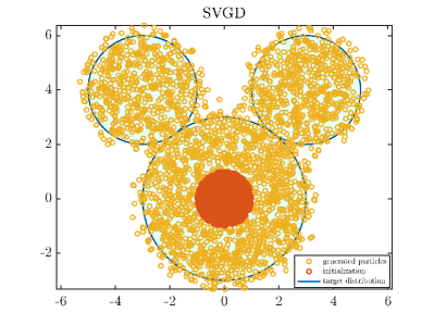
Figure 1. Mickey mouse: 2700 generated particles using DPMS and SVGD, with 2000 training samples

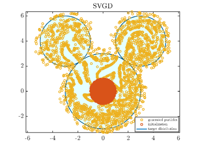
Figure 2. Mickey mouse: an instance of running the SVGD generative model shows strange non-uniform pattern with 1000 training samples and 2700 generated particles

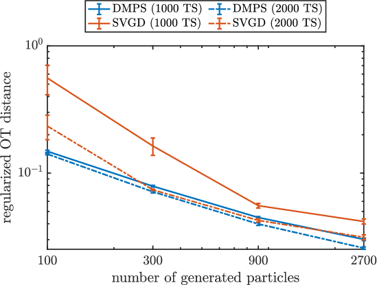
Figure 3. Mickey mouse: error comparison between DMPS, SVGD

8.2. Two moons: two-dimensional disconnected domain

In this example, the target distribution is uniform and compactly supported on a two-moon-shaped domain. In contrast with the previous example, the domain is disconnected. Though the underlying distribution has zero density outside the support, the finite kernel bandwidth enables the methods to be implementable in this case. Results are obtained with $500$ and $1000$ training samples. We show the initial particles, target distribution, and particles generated with DMPS, SVGD, and ULA in Figure 4 and the regularized OT distance in Figure 5. As we can see in Figure 4, SVGD does not explore the very end of the domain and ULA has mny samples that diffuse out of the support. The error plot (Figure 5) shows that DMPS enjoys the smallest error in terms of OT distance, and that this the error decreases with more generated particles. While ULA shows a similar convergence (with larger values of error), the error of SVGD fluctuates as more particles are included.

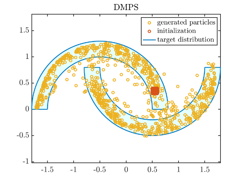
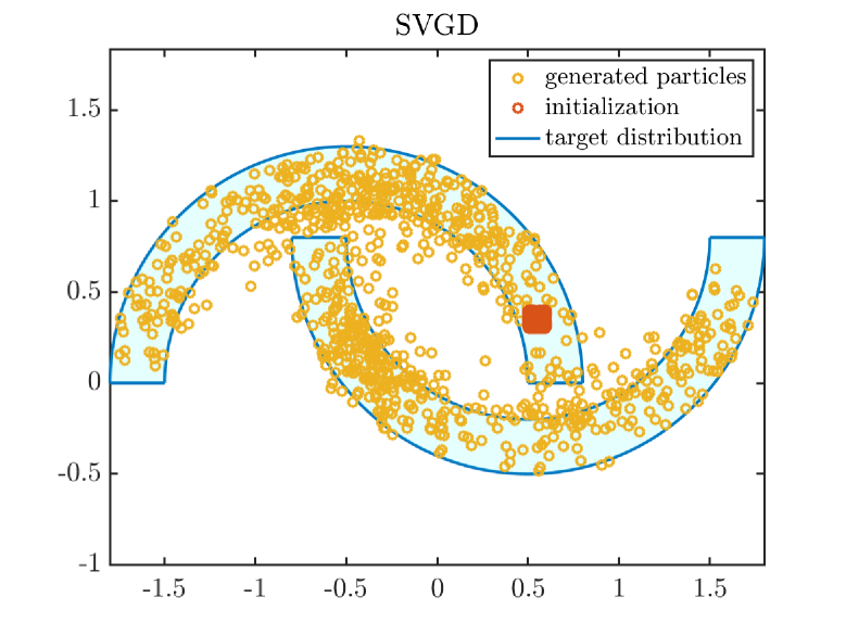
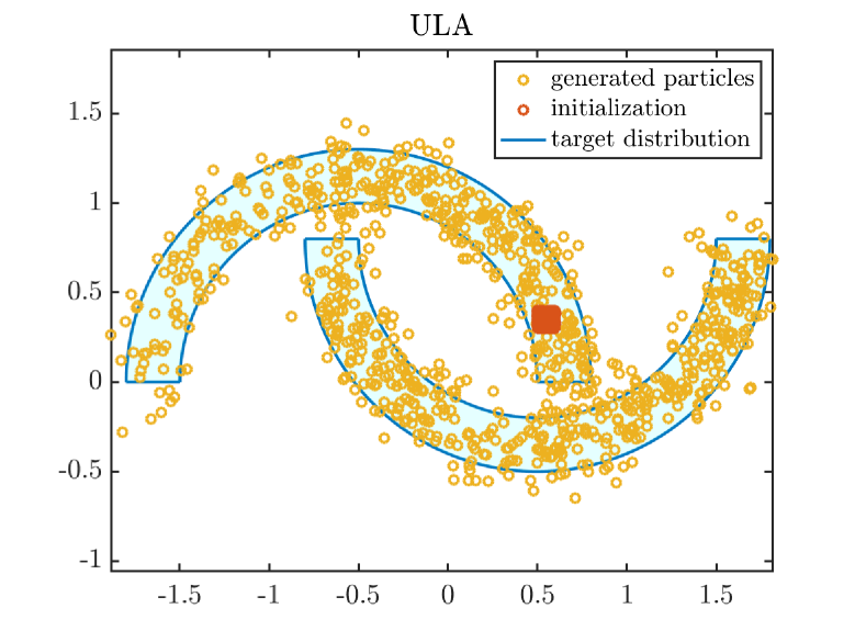
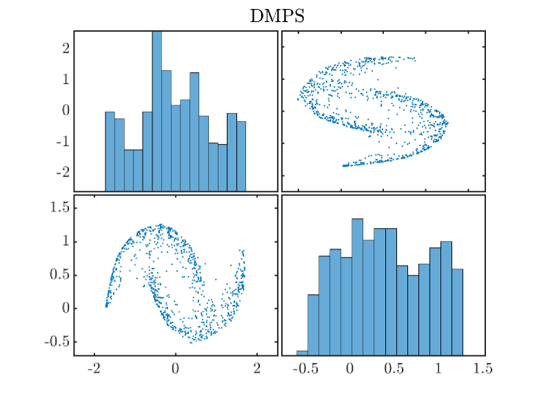
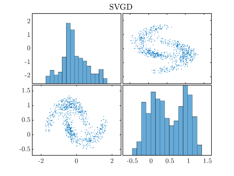
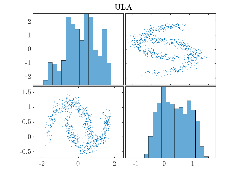
Figure 4. Two moons: 900 generated particles from DMPS, SVGD, and ULA with 500 training samples

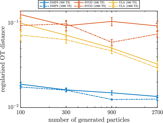
Figure 5. Two moons: error comparison between DMPS, SVGD, and ULA. Solid lines use 500 training samples, dashed lines use 1000.

8.3. The arc: one-dimensional manifold embedded in a three-dimensional space

We now consider an example where the data lie on a manifold, in this case an arc of radius $1$ embedded in $\mathbb{R}^{3}$. Training data are drawn uniformly from the arc and perturbed in the radial direction only, with $U(0,10^{-2})$ noise. Results are obtained with both 100 and 1000 training samples. The initial particles and the target distribution are shown in Figure 6 (left). We then run DMPS, SVGD, ULA, and SGM for each batch of training and initialization samples, visualizing an instance in Figure 6. Particles generated by the two deterministic methods, DMPS and SVGD, lie only on the two-dimensional plane of the training data, but the particles generated using SVGD do not fully explore the target distribution. Particles generated by the two stochastic methods, ULA and SGM, span the full three-dimensional space due to the added noise. Errors are plotted in Figure 7, for both choices of training set size. We see that DMPS exhibits the smallest errors, and that this error decreases as we increase the number of generated particles. SGM shows a similar trend, but with larger errors. The performance of ULA does not seem to improve after using more training samples, which might be due to finite discretization timestep (although it was chosen small relative to the width of the target, $h=5\times 10^{-4}$). SVGD gives the largest errors, which do not seem to decrease with more particles.

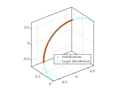
(a) Initialization and target distribution

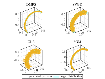
(b) Generated particles

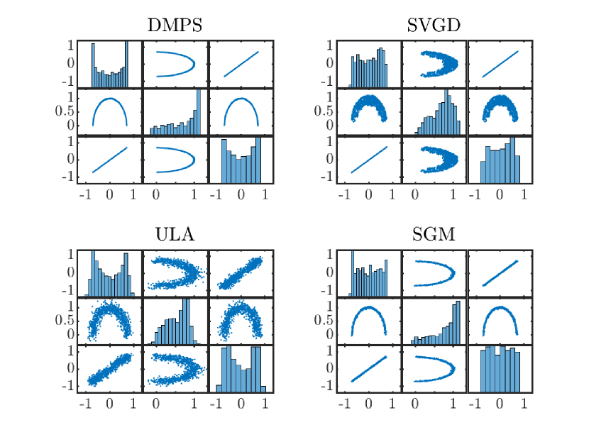
(c) Marginal distributions

Figure 6. The arc: 900 generated particles using DMPS, SVGD, ULA, and SGM with 1000 training samples.

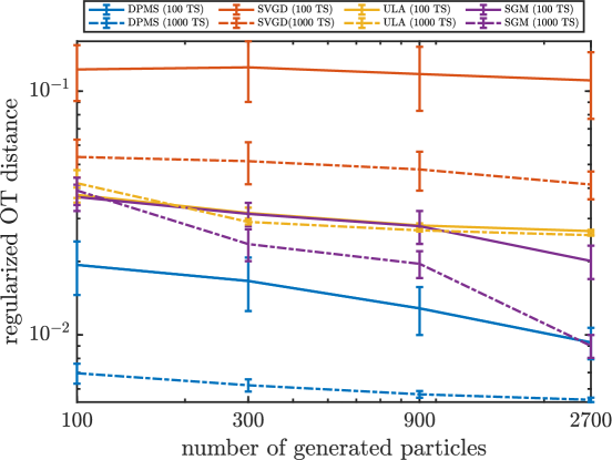
Figure 7. The arc: error comparison between DMPS, SVGD, ULA, and SGM. Solid lines use 100 training samples; dashed lines use 1000.

8.4. Hyper-semisphere: 2 to 14-dimensional manifolds

We finally study an example where data are uniformly sampled on a half-sphere embedded in ambient dimensions $d\in\{3,6,9,12,15\}$; in each case, the manifold is thus of dimension $d-1$. For this problem, the number of training samples and the number of generated particles are fixed to $1000$ and $300$, respectively. A visualization for $d=3$ can be seen in Figure 8. We show the error (in OT distance), and the standard error of the mean error over 10 trials, in Table 1. For all dimensions, DMPS enjoys the smallest error and the smallest standard error, followed by SGM and ULA, which also produce relatively small errors and stable results. SVGD has the largest error and does not produce stable results (large variability over the 10 trials).

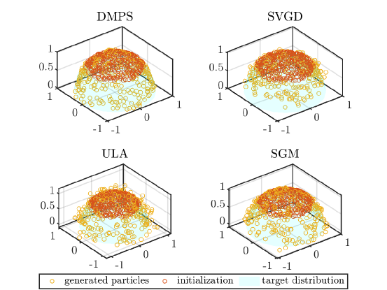
Figure 8. Hyper-semisphere: 300 generated samples using DMPS, SVGD, ULA and SGM in three dimensions with 1000 training samples.

	DMPS	SVGD	ULA	SGM
$d$ = 3	0.018 $\pm$ 0.0003	0.146 $\pm$ 0.0229	0.033 $\pm$ 0.0006	0.032 $\pm$ 0.0024
$d$ = 6	0.142 $\pm$ 0.0003	0.267 $\pm$ 0.0171	0.185 $\pm$ 0.0012	0.170 $\pm$ 0.0022
$d$ = 9	0.303 $\pm$ 0.0003	0.361 $\pm$ 0.0077	0.378 $\pm$ 0.0011	0.348 $\pm$ 0.0025
$d$ = 12	0.441 $\pm$ 0.0002	0.811 $\pm$ 0.0783	0.555 $\pm$ 0.0018	0.496 $\pm$ 0.0041
$d$ = 15	0.564 $\pm$ 0.0009	0.986 $\pm$ 0.0055	0.713 $\pm$ 0.0025	0.608 $\pm$ 0.0024

Table 1. Hyper-semisphere: error comparison ($\pm$ standard error) between DMPS, SVGD, ULA, and SGM.

8.5. High energy physics: gluon jet dataset

We now study a real-world example from high energy physics, where the goal is to generate relative angular coordinates $\eta^{\textrm{rel}},\phi^{\textrm{rel}}$ and relative transverse momenta $p_{T}^{\textrm{rel}}$ of elementary physical particles produced in a gluon jet. Details on the dataset are in Kansal et al. (2021). The dataset is of dimension $177252\times 30\times 4$, meaning that there are $177252$ jets, $30$ physical particles per jet and each particle is characterized by four distinct features: $\eta^{\textrm{rel}}$, $\phi^{\textrm{rel}}$, $p_{T}^{\textrm{rel}}$, and a binary mask. Since the value of the last feature is either $0$ or $1$, we only use the first three features for the propose of generative modeling. Therefore, for each physical particle, there are $177252$ available samples, and each sample is of $3$ dimensions. We then train a generative model for each of the $30$ physical particles. To train each model, we normalize the training data so that they have mean zero and marginal variances of one. We use $1000$ samples for training, which are drawn randomly from the full set of $177252$ samples, and initialize 100, 300, 900, or 2700 samples from $U(-1,1)^{3}$ for the generative process. We also compare SVGD, ULA and SGM with the same setup: 1000 training samples and increasing numbers of generated samples. Errors ($\pm$ standard error) for all four methods are shown in Table 2. These results are averaged over all $30$ different physical particles. We see that DMPS consistently outperforms the other methods across all cases in this problem. In Figure 9, we also show the marginal distributions of 2700 generated samples (in red) using different methods and plot target samples (in blue) as a reference, for the first physical particle. As we can see, samples generated using DMPS, ULA, and SGM resemble those from the target distribution. Samples generated using SVGD, however, qualitatively fail to capture the target distribution, consistent with the larger errors in Table 2.

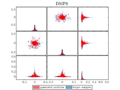
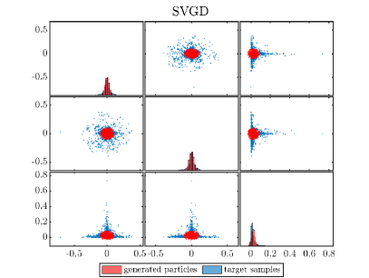
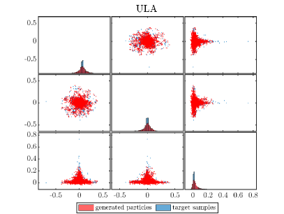
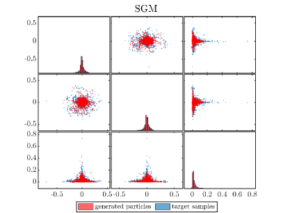
Figure 9. Gluon jet dataset: marginal distributions of the target samples and 2700 generated particles using DMPS, SVGD, ULA, and SGM with 1000 traning samples. Coordinates are $\eta^{\textrm{rel}}$, $\phi^{\textrm{rel}}$, and $p_{T}^{\textrm{rel}}$, respectively.

# particles	DMPS	SVGD	ULA	SGM
100	$\bm{0.0020}$ ${\pm 5.03\times 10^{-5}}$	$0.0062\newline \pm 4.00\times 10^{-4}$	$0.0041\newline \pm 2.64\times 10^{-4}$	$0.0029\newline \pm 1.21\times 10^{-4}$
300	$\bm{0.0014}$ ${\pm 1.65\times 10^{-5}}$	$0.0059\newline \pm 3.75\times 10^{-4}$	$0.0032\newline \pm 1.73\times 10^{-4}$	$0.0021\newline \pm 0.55\times 10^{-4}$
900	$\bm{0.0012}$ ${\pm 1.61\times 10^{-5}}$	$0.0058\newline \pm 3.65\times 10^{-4}$	$0.0029\newline \pm 1.53\times 10^{-4}$	$0.0018\newline \pm 0.46\times 10^{-4}$
2700	$\bm{0.0012}$ ${\pm 1.59\times 10^{-5}}$	$0.0057\newline \pm 3.61\times 10^{-4}$	$0.0027\newline \pm 1.30\times 10^{-4}$	$0.0018\newline \pm 0.44\times 10^{-4}$

Table 2. Gluon jet dataset: error comparison ($\pm$ standard error) between DMPS, SVGD, ULA, and SGM, for different numbers of generated particles.

8.6. Remarks on the experiments

In these experiments, we see that for all methods the error decreases with more training samples, and that the error of DMPS, ULA, and SGM decreases with more generated particles. We also observe that DMPS has the best performance in terms of the regularized OT metric. The reason might be that the kernel method for approximating the generator relies on diffusion maps, or more broadly, the graph Laplacian, which is widely used for manifold learning due to its flexibility in detecting the underlying geometry. The fact that the generator is approximated as a whole distinguishes it from other score-based methods.

Although the gradient of the potential term is approximated in the same fashion in our SVGD approach, performance might be affected by the interaction between two kernels: one from the diffusion map approximation and the other being the kernel of the SVGD algorithm itself, as well as the choice of the kernel bandwidths. Performance is more stable for the two non-deterministic methods, ULA and SGM, compared to SVGD. For ULA, since Gaussian noise is added at in every step, particles are able to “leave” the manifold for any finite stepsize. On the other hand, SGM produces generally good results. However, it does suffer from having longer training times. For the arc problem, with $1000$ training samples and $100$ initial particles, DMPS took $6.21$ seconds while SGM (trained using 5000 epochs) took $1633$ seconds ($27$ minutes).

9. Conclusion

We introduced DMPS as a simple-to-implement and computationally efficient kernel method for generative modeling. Our approach combines diffusion maps with the LAWGD approach to construct a generative particle system that adapts to the geometry of the underlying distribution. Our method compares favorably with other competing schemes (SVGD and ULA with learned scores, and diffusion-based generative models) on synthetic datasets, consistently achieving the smallest errors in terms of regularized OT distance. While the examples presented here are of moderate dimension (up to $d=15$ for the example in Section 8.4), we expect that more sophisticated kernel methods Li et al. (2017) can slot naturally into the DMPS framework and help extend the method to higher-dimensional problems. Future research will also study the convergence rate of the method in discrete time and with finite samples, and consider more complex geometric domains.

Appendix A Spectral properties of $\mathscr{L}$

Suppose $\mathcal{D}$ is compact and $\mathscr{L}=-\nabla^{2}+\langle\nabla V,\nabla\cdot\rangle$ has discrete spectrum $\{\sigma_{i}\}_{i=1}^{\infty}$. Then the spectrum is bounded $\sigma_{0}=0\leq\sigma_{1}\leq\sigma_{2}\leq\cdots\leq B<\infty$ [Shi, 2020]. Let $\phi_{i}$ be the corresponding eigenfunctions. The action of $\mathscr{L}$ on a function $f\in L^{2}(\pi)$ reads

$$\mathscr{L}f(x)=\sum_{i=1}^{\infty}\sigma_{i}\langle\phi_{i},f\rangle_{L^{2}(\pi)}\phi_{i}(x),$$

and its inverse has the following expression

$$\mathscr{L}^{-1}f(x)=\sum_{i=1}^{\infty}\sigma_{i}^{-1}\langle\phi_{i},f\rangle_{L^{2}(\pi)}\phi_{i}(x).$$

Appendix B Finite sample approximation of the operator

In this section, we introduce the finite sample counterpart to the approximations in Section 4.1. We consider the approximation of the generator of the Langevin diffusion process $\mathscr{L}$ from finite samples $\{z^{i}\}_{i=1}^{N}\sim\pi$. In this case, we have

$$M_{\epsilon,N}(x,y)=\frac{K_{\epsilon}(x,y)}{\sqrt{\sum_{i=1}^{N}K_{\epsilon}(z^{i},y)}\sqrt{\sum_{i=1}^{N}K_{\epsilon}(x,z^{i})}},$$

and the corresponding $L_{\epsilon,N}^{f}$ and $L_{\epsilon,N}^{b}$ can be written as

$$P_{\epsilon,N}^{f}(x,y):=\frac{M_{\epsilon,N}(x,y)}{\sum_{i=1}^{N}M_{\epsilon,N}(z^{i},y)},$$

$$P_{\epsilon,N}^{b}(x,y):=\frac{M_{\epsilon,N}(x,y)}{\sum_{i=1}^{N}M_{\epsilon,N}(x,z^{i})},$$

and we set

(B.1) $$P_{\epsilon,N}(x,y)=\frac{1}{2}\left(P_{\epsilon,N}^{f}(x,y)+P_{\epsilon,N}^{b}(x,y)\right).$$

Similarly, its action on a function $g$ writes

$$T^{f,b}_{\epsilon,N}g(x)=\sum_{i=1}^{N}P^{f,b}_{\epsilon,N}(x,z^{i})g(z^{i}).$$

Let

$$L^{f,b}_{\epsilon,N}:=\frac{\mathrm{Id}-T^{f,b}_{\epsilon,N}}{\epsilon}.$$

Similar to their spatial continuum limit, we have

$$\lim_{\epsilon\rightarrow 0,N\rightarrow\infty}L^{f}_{\epsilon,N}=\lim_{\epsilon\rightarrow 0,N\rightarrow\infty}L^{b}_{\epsilon,N}=\mathscr{L}.$$

Then, similar to (4.1), we have that

$$\lim_{\epsilon\rightarrow 0,N\rightarrow\infty}\frac{g(x)-\sum_{i=1}^{N}P^{f,b}_{\epsilon,N}(x,z^{i})g(z^{i})}{\epsilon}=\mathscr{L}g(x),$$

and

$$L_{\epsilon,N}=\frac{1}{2}(L_{\epsilon,N}^{f}+L_{\epsilon,N}^{b}).$$

is the symmetric kernel.

B.1. Computing $\nabla_{1}P_{\epsilon}(x,y)$

Recall that $P_{\epsilon}=\frac{1}{2}(P_{\epsilon}^{f}+P_{\epsilon}^{b})$. We then compute $\nabla_{1}P_{\epsilon}^{f}(x,y)$ and $\nabla_{1}P_{\epsilon}^{b}(x,y)$ separately.

B.1.1. Computing $\nabla_{1}P^{f}_{\epsilon}(x,y)$

Recall

$$P_{\epsilon}^{f}(x,y):=\frac{M_{\epsilon}(x,y)}{\int_{X}M_{\epsilon}(x,y)d\pi(x)},$$

where

(B.2) $$M_{\epsilon}(x,y):=\frac{K_{\epsilon}(x,y)}{\sqrt{\int_{\mathcal{X}}K_{\epsilon}(x,y)d\pi(x)}\sqrt{\int_{\mathcal{Y}}K_{\epsilon}(x,y)d\pi(y)}}.$$

Then

$$\nabla_{1}P_{\epsilon}^{f}(x,y)=\frac{\nabla_{1}M_{\epsilon}(x,y)}{\int_{X}M_{\epsilon}(x,y)d\pi(x)}.$$

We then compute $\nabla_{1}M_{\epsilon}(x,y)$. Let $d_{\epsilon}(x)=\int_{\mathcal{Y}}K_{\epsilon}(x,y)d\pi(y)$ and $d_{\epsilon}(y)=\int_{\mathcal{X}}K_{\epsilon}(x,y)d\pi(x)$, then

$$\nabla_{1}M_{\epsilon}(x,y)=\frac{\nabla_{1}K_{\epsilon}(x,y)\sqrt{d_{\epsilon}(y)}\sqrt{d_{\epsilon}(x)}-\left(\frac{\partial}{\partial x}\sqrt{d_{\epsilon}(x)}\right)\sqrt{d_{\epsilon}(y)}K_{\epsilon}(x,y)}{d_{\epsilon}(x)d_{\epsilon}(y)},$$

where

(B.3) $$\nabla_{1}K_{\epsilon}(x,y) =-\left(\frac{x-y}{\epsilon}\right)e^{-\frac{\left\|x-y\right\|^{2}}{2\epsilon}},$$

(B.4) $$\frac{\partial}{\partial x}\left(\sqrt{d_{\epsilon}(x)}\right) =\frac{1}{2}\int_{\mathcal{Y}}\left(-\left(\frac{x-y}{\epsilon}\right)e^{-\frac{\left\|x-y\right\|^{2}}{2\epsilon}}\right)^{-1/2}d\pi(y).$$

B.1.2. Computing $\nabla_{1}P_{\epsilon}^{b}(x,y)$

On the other hand, we have

$$P_{\epsilon}^{b}(x,y):=\frac{M_{\epsilon}(x,y)}{\int_{\mathcal{Y}}M_{\epsilon}(x,y)d\pi(y)},$$

and

$$\nabla_{1}P_{\epsilon}^{b}(x,y)=\frac{\nabla_{1}M_{\epsilon}(x,y)\int_{\mathcal{Y}}M_{\epsilon}(x,y)d\pi(y)-\int_{\mathcal{Y}}\nabla_{1}M_{\epsilon}(x,y)d\pi(y)M_{\epsilon}(x,y)}{\left(\int_{\mathcal{Y}}M_{\epsilon}(x,y)d\pi(y)\right)^{2}},$$

where all the ingredients are computable from (B.2), (B.3), and (B.4).

B.2. Computing $\nabla_{1}P_{\epsilon,N}(x,y)$

The discrete version is obtained by replacing the integral with its empirical average. Similarly, let $\{z^{i}\}_{i=1}^{N}\sim\pi$, and define $d_{\epsilon,N}(x)=\sum_{i=1}^{N}K_{\epsilon}(x,z^{i})$ and $d_{\epsilon,N}(y)=\sum_{i=1}^{N}K_{\epsilon}(z^{i},y)$. Recall that

$$M_{\epsilon,N}(x,y)=\frac{K_{\epsilon}(x,y)}{\sqrt{\sum_{i=1}^{N}K_{\epsilon}(z^{i},y)}\sqrt{\sum_{i=1}^{N}K_{\epsilon}(x,z^{i})}}.$$

Then

$$\nabla_{1}M_{\epsilon,N}(x,y)=\frac{\nabla_{1}K_{\epsilon,N}(x,y)\sqrt{d_{\epsilon,N}(y)}\sqrt{d_{\epsilon,N}(x)}-\left(\frac{\partial}{\partial x}\sqrt{d_{\epsilon,N}(x)}\right)\sqrt{d_{\epsilon,N}(y)}K_{\epsilon}(x,y)}{d_{\epsilon,N}(x)d_{\epsilon,N}(y)},$$

and

$$\frac{\partial}{\partial x}\left(\sqrt{d_{\epsilon,N}(x)}\right) =\frac{1}{2}\sum_{i=1}^{N}\left(-\left(\frac{x-z^{i}}{\epsilon}\right)e^{-\frac{\left\|x-z^{i}\right\|^{2}}{2\epsilon}}\right)^{-1/2}.$$

Finally, similar to the previous section, we have that

$$\nabla_{1}P_{\epsilon,N}^{f}(x,y)=\frac{\nabla_{1}M_{\epsilon,N}(x,y)}{\sum_{i=1}^{N}M_{\epsilon,N}(z^{i},y)},$$

and

$$\nabla_{1}P_{\epsilon,N}^{b}(x,y)=\frac{\nabla_{1}M_{\epsilon,N}(x,y)\left(\sum_{i=1}^{N}M_{\epsilon,N}(x,z^{i})\right)-\left(\sum_{i=1}^{N}\nabla_{1}M_{\epsilon,N}(x,z^{i})\right)M_{\epsilon,N}(x,y)}{\left(\sum_{i=1}^{N}M_{\epsilon,N}(x,z^{i})\right)^{2}}.$$

Appendix C Regularity assumptions

We state here the regularity assumptions needed for the gradient to converge. The statement and the proof are adapted from Peres .

Theorem C.1.

Suppose $L_{\epsilon}f(x)$ is a family of bounded differentiable functions from $\mathcal{D}$ to $\mathbb{R}$ converging pointwise to $\mathscr{L}f(x)$ as $\epsilon\rightarrow 0$. Furthermore, suppose $\nabla L_{\epsilon}f(x)$ is a family of uniformly equicontinuous functions. Then $\mathscr{L}f(x)$ is differentiable on $\mathcal{D}$ and $\nabla L_{\epsilon}f(x)$ converges to $\nabla\mathscr{L}f(x)$ uniformly.

Proof.

We first choose a countable set of $\epsilon$, say, $\epsilon=\{1/n\}_{i=1}^{\infty}$, and we use $L_{n}$ to denote $L_{\epsilon=1/n}$ for convenience. Since $L_{n}f(x)$ are uniformly bounded and $\nabla L_{n}f(x)$ are uniformly equicontinuous, $\nabla L_{n}f(x)$ are uniformly bounded. Then $\nabla L_{n}f(x)$ has a subsequence $\nabla L_{n(k)}f(x)$ that converges uniformly to some function $g\in C(\mathcal{D})$ by the Arzela-Ascoli theorem. We then show that $g=\nabla\mathscr{L}f(x)$ by contradiction. Suppose $\nabla L_{n}f(x)$ does not converge uniformly to $\nabla\mathscr{L}f(x)$. Then there exists $\epsilon>0$ and another subsequence $\nabla L_{m(k)}f(x)$ of $\nabla L_{n}f(x)$ such that $\|\nabla L_{m(k)}f-\nabla\mathscr{L}f\|_{\infty}>\epsilon$ for all $k$. But by the Arzela-Ascoli theorem, $\nabla L_{m(k)}$ has a subsequence converging uniformly to $\nabla\mathscr{L}f(x)$: contradiction. Therefore, $\nabla L_{n}f(x)$ converges to $\nabla\mathscr{L}f(x)$ uniformly on $\mathcal{D}$. ∎

References

- Adams et al. [2013] Stefan Adams, Nicolas Dirr, Mark Peletier, and Johannes Zimmer. Large deviations and gradient flows. Philosophical transactions. Series A, Mathematical, physical, and engineering sciences, 371:20120341, 11 2013. doi: 10.1098/rsta.2012.0341.
- Ambrosio et al. [2005] Luigi Ambrosio, Nicola Gigli, and Giuseppe Savare. Gradient flows in metric spaces and in the space of probability measures. 01 2005. doi: 10.1007/978-3-7643-8722-8.
- Anand and Huang [2018] Namrata Anand and Possu Huang. Generative modeling for protein structures. In S. Bengio, H. Wallach, H. Larochelle, K. Grauman, N. Cesa-Bianchi, and R. Garnett, editors, Advances in Neural Information Processing Systems, volume 31. Curran Associates, Inc., 2018. URL https://proceedings.neurips.cc/paper/2018/file/afa299a4d1d8c52e75dd8a24c3ce534f-Paper.pdf.
- Belkin and Niyogi [2003] Mikhail Belkin and Partha Niyogi. Laplacian eigenmaps for dimensionality reduction and data representation. Neural Computation, 15(6):1373–1396, 2003. doi: 10.1162/089976603321780317.
- Bortoli et al. [2022] Valentin De Bortoli, Emile Mathieu, Michael Hutchinson, James Thornton, Yee Whye Teh, and A. Doucet. Riemannian score-based generative modeling. ArXiv, abs/2202.02763, 2022.
- Brehmer and Cranmer [2020] Johann Brehmer and Kyle Cranmer. Flows for simultaneous manifold learning and density estimation. ArXiv, abs/2003.13913, 2020.
- Cai et al. [2020] Ruojin Cai, Guandao Yang, Hadar Averbuch-Elor, Zekun Hao, Serge J. Belongie, Noah Snavely, and Bharath Hariharan. Learning gradient fields for shape generation. In Andrea Vedaldi, Horst Bischof, Thomas Brox, and Jan-Michael Frahm, editors, Computer Vision - ECCV 2020 - 16th European Conference, Glasgow, UK, August 23-28, 2020, Proceedings, Part III, volume 12348 of Lecture Notes in Computer Science, pages 364–381. Springer, 2020. doi: 10.1007/978-3-030-58580-8“˙22. URL https://doi.org/10.1007/978-3-030-58580-8_22.
- Caterini et al. [2021] Anthony L. Caterini, Gabriel Loaiza-Ganem, Geoff Pleiss, and John P. Cunningham. Rectangular flows for manifold learning. In Neural Information Processing Systems, 2021.
- Chewi et al. [2020] Sinho Chewi, Thibaut Le Gouic, Chen Lu, Tyler Maunu, and Philippe Rigollet. Svgd as a kernelized wasserstein gradient flow of the chi-squared divergence. ArXiv, abs/2006.02509, 2020.
- Coifman et al. [2005] R. R. Coifman, S. Lafon, A. B. Lee, M. Maggioni, B. Nadler, F. Warner, and S. W. Zucker. Geometric diffusions as a tool for harmonic analysis and structure definition of data: Diffusion maps. Proceedings of the National Academy of Sciences, 102(21):7426–7431, 2005. doi: 10.1073/pnas.0500334102. URL https://www.pnas.org/doi/abs/10.1073/pnas.0500334102.
- Coifman and Lafon [2006] Ronald R. Coifman and Stéphane Lafon. Diffusion maps. Applied and Computational Harmonic Analysis, 21(1):5–30, 2006. ISSN 1063-5203. doi: https://doi.org/10.1016/j.acha.2006.04.006. URL https://www.sciencedirect.com/science/article/pii/S1063520306000546. Special Issue: Diffusion Maps and Wavelets.
- Cuturi [2013] Marco Cuturi. Sinkhorn distances: Lightspeed computation of optimal transport. In C.J. Burges, L. Bottou, M. Welling, Z. Ghahramani, and K.Q. Weinberger, editors, Advances in Neural Information Processing Systems, volume 26. Curran Associates, Inc., 2013. URL https://proceedings.neurips.cc/paper/2013/file/af21d0c97db2e27e13572cbf59eb343d-Paper.pdf.
- Daneri and Savaré [2010] Sara Daneri and Giuseppe Savaré. Lecture notes on gradient flows and optimal transport, 2010. URL https://arxiv.org/abs/1009.3737.
- Franzese et al. [2022] Giulio Franzese, Simone Rossi, Lixuan Yang, Alessandro Finamore, Dario Rossi, Maurizio Filippone, and Pietro Michiardi. How much is enough? a study on diffusion times in score-based generative models, 2022. URL https://arxiv.org/abs/2206.05173.
- Garbuno-Iñigo et al. [2019] Alfredo Garbuno-Iñigo, Nikolas Nüsken, and Sebastian Reich. Affine invariant interacting langevin dynamics for bayesian inference. SIAM J. Appl. Dyn. Syst., 19:1633–1658, 2019.
- Goodfellow et al. [2014] Ian Goodfellow, Jean Pouget-Abadie, Mehdi Mirza, Bing Xu, David Warde-Farley, Sherjil Ozair, Aaron Courville, and Yoshua Bengio. Generative adversarial nets. In Z. Ghahramani, M. Welling, C. Cortes, N. Lawrence, and K.Q. Weinberger, editors, Advances in Neural Information Processing Systems, volume 27. Curran Associates, Inc., 2014. URL https://proceedings.neurips.cc/paper/2014/file/5ca3e9b122f61f8f06494c97b1afccf3-Paper.pdf.
- Hein et al. [2005] Matthias Hein, Jean-Yves Audibert, and Ulrike von Luxburg. From graphs to manifolds - weak and strong pointwise consistency of graph laplacians. In Annual Conference Computational Learning Theory, 2005.
- Ho et al. [2019] Jonathan Ho, Xi Chen, A. Srinivas, Yan Duan, and P. Abbeel. Flow++: Improving flow-based generative models with variational dequantization and architecture design. ArXiv, abs/1902.00275, 2019.
- Ho et al. [2020] Jonathan Ho, Ajay Jain, and Pieter Abbeel. Denoising diffusion probabilistic models. In H. Larochelle, M. Ranzato, R. Hadsell, M.F. Balcan, and H. Lin, editors, Advances in Neural Information Processing Systems, volume 33, pages 6840–6851. Curran Associates, Inc., 2020. URL https://proceedings.neurips.cc/paper/2020/file/4c5bcfec8584af0d967f1ab10179ca4b-Paper.pdf.
- Ho et al. [2021] Jonathan Ho, Chitwan Saharia, William Chan, David J. Fleet, Mohammad Norouzi, and Tim Salimans. Cascaded diffusion models for high fidelity image generation. J. Mach. Learn. Res., 23:47:1–47:33, 2021.
- Jordan et al. [1998] Richard Jordan, David Kinderlehrer, and Felix Otto. The variational formulation of the fokker–planck equation. SIAM Journal on Mathematical Analysis, 29(1):1–17, 1998. doi: 10.1137/S0036141096303359. URL https://doi.org/10.1137/S0036141096303359.
- Kansal et al. [2021] Raghav Kansal, Javier Duarte, Hao Su, Breno Orzari, Thiago Tomei, Maurizio Pierini, Mary Touranakou, Dimitrios Gunopulos, et al. Particle cloud generation with message passing generative adversarial networks. Advances in Neural Information Processing Systems, 34:23858–23871, 2021.
- Kazeminia et al. [2020] Salome Kazeminia, Christoph Baur, Arjan Kuijper, Bram van Ginneken, Nassir Navab, Shadi Albarqouni, and Anirban Mukhopadhyay. Gans for medical image analysis. Artificial Intelligence in Medicine, 109:101938, 2020. ISSN 0933-3657. doi: https://doi.org/10.1016/j.artmed.2020.101938. URL https://www.sciencedirect.com/science/article/pii/S0933365719311510.
- Khandelwal and Krishnan [2019] Arjun Khandelwal and Rahul G. Krishnan. Fine-tuning generative models. 2019.
- Kingma and Welling [2013] Diederik P. Kingma and Max Welling. Auto-encoding variational bayes. CoRR, abs/1312.6114, 2013.
- Knight [2008] Philip A. Knight. The sinkhorn-knopp algorithm: Convergence and applications. SIAM J. Matrix Anal. Appl., 30:261–275, 2008.
- Li et al. [2017] Chun-Liang Li, Wei-Cheng Chang, Yu Cheng, Yiming Yang, and Barnabás Póczos. MMD GAN: Towards deeper understanding of moment matching network. In NIPS, 2017.
- Li et al. [2022] Xiang Lisa Li, John Thickstun, Ishaan Gulrajani, Percy Liang, and Tatsunori B. Hashimoto. Diffusion-lm improves controllable text generation, 2022. URL https://arxiv.org/abs/2205.14217.
- Li et al. [2018] Yang Li, Quan Pan, Suhang Wang, Tao Yang, and Erik Cambria. A generative model for category text generation. Information Sciences, 450:301–315, 2018. ISSN 0020-0255. doi: https://doi.org/10.1016/j.ins.2018.03.050. URL https://www.sciencedirect.com/science/article/pii/S0020025518302366.
- Liu [2017] Qiang Liu. Stein variational gradient descent as gradient flow. In I. Guyon, U. Von Luxburg, S. Bengio, H. Wallach, R. Fergus, S. Vishwanathan, and R. Garnett, editors, Advances in Neural Information Processing Systems, volume 30. Curran Associates, Inc., 2017. URL https://proceedings.neurips.cc/paper/2017/file/17ed8abedc255908be746d245e50263a-Paper.pdf.
- Liu and Wang [2016] Qiang Liu and Dilin Wang. Stein variational gradient descent: A general purpose bayesian inference algorithm. In NIPS, 2016.
- Mahapatra et al. [2019] Dwarikanath Mahapatra, Behzad Bozorgtabar, and Rahil Garnavi. Image super-resolution using progressive generative adversarial networks for medical image analysis. Computerized Medical Imaging and Graphics, 71:30–39, 2019. ISSN 0895-6111. doi: https://doi.org/10.1016/j.compmedimag.2018.10.005. URL https://www.sciencedirect.com/science/article/pii/S0895611118305871.
- Miao and Blunsom [2016] Yishu Miao and Phil Blunsom. Language as a latent variable: Discrete generative models for sentence compression. pages 319–328, 01 2016. doi: 10.18653/v1/D16-1031.
- Nadler et al. [2005] Boaz Nadler, Stephane Lafon, Ioannis Kevrekidis, and Ronald Coifman. Diffusion maps, spectral clustering and eigenfunctions of fokker-planck operators. In Y. Weiss, B. Schölkopf, and J. Platt, editors, Advances in Neural Information Processing Systems, volume 18. MIT Press, 2005. URL https://proceedings.neurips.cc/paper/2005/file/2a0f97f81755e2878b264adf39cba68e-Paper.pdf.
- Nadler et al. [2006] Boaz Nadler, Stéphane Lafon, Ronald R. Coifman, and Ioannis G. Kevrekidis. Diffusion maps, spectral clustering and reaction coordinates of dynamical systems. Applied and Computational Harmonic Analysis, 21(1):113–127, 2006. ISSN 1063-5203. doi: https://doi.org/10.1016/j.acha.2005.07.004. URL https://www.sciencedirect.com/science/article/pii/S1063520306000534. Special Issue: Diffusion Maps and Wavelets.
- Nie et al. [2017] Dong Nie, Roger Trullo, Jun Lian, Caroline Petitjean, Su Ruan, Qian Wang, and Dinggang Shen. Medical image synthesis with context-aware generative adversarial networks. In Maxime Descoteaux, Lena Maier-Hein, Alfred Franz, Pierre Jannin, D. Louis Collins, and Simon Duchesne, editors, Medical Image Computing and Computer Assisted Intervention (MICCAI 2017), pages 417–425, Cham, 2017. Springer International Publishing.
- [37] Yuval Peres. Conditions for convergence of a derivative, given the function itself is convergent. Mathematics Stack Exchange. URL https://math.stackexchange.com/q/4517640. (version: 2022-08-24).
- Pidstrigach [2022a] Jakiw Pidstrigach. Score-based generative models detect manifolds. ArXiv, abs/2206.01018, 2022a.
- Pidstrigach [2022b] Jakiw Pidstrigach. Score-based generative models introduction. https://jakiw.com/sgm_intro, 2022b. Accessed: 2024-01-24.
- Ranzato et al. [2011] Marc’Aurelio Ranzato, Joshua Susskind, Volodymyr Mnih, and Geoffrey Hinton. On deep generative models with applications to recognition. In CVPR 2011, pages 2857–2864, 2011. doi: 10.1109/CVPR.2011.5995710.
- Rezende et al. [2014] Danilo Jimenez Rezende, Shakir Mohamed, and Daan Wierstra. Stochastic backpropagation and approximate inference in deep generative models. In Eric P. Xing and Tony Jebara, editors, Proceedings of the 31st International Conference on Machine Learning, volume 32 of Proceedings of Machine Learning Research, pages 1278–1286, Bejing, China, 22–24 Jun 2014. PMLR. URL https://proceedings.mlr.press/v32/rezende14.html.
- Rombach et al. [2021] Robin Rombach, Andreas Blattmann, Dominik Lorenz, Patrick Esser, and Björn Ommer. High-resolution image synthesis with latent diffusion models, 2021. URL https://arxiv.org/abs/2112.10752.
- Roweis and Saul [2000] Sam T. Roweis and Lawrence K. Saul. Nonlinear dimensionality reduction by locally linear embedding. Science, 290 5500:2323–6, 2000.
- Ruthotto and Haber [2021] Lars Ruthotto and Eldad Haber. An introduction to deep generative modeling. GAMM-Mitteilungen, 44(2):e202100008, 2021. doi: https://doi.org/10.1002/gamm.202100008. URL https://onlinelibrary.wiley.com/doi/abs/10.1002/gamm.202100008.
- Salimans et al. [2016] Tim Salimans, Ian Goodfellow, Wojciech Zaremba, Vicki Cheung, Alec Radford, Xi Chen, and Xi Chen. Improved techniques for training gans. In D. Lee, M. Sugiyama, U. Luxburg, I. Guyon, and R. Garnett, editors, Advances in Neural Information Processing Systems, volume 29. Curran Associates, Inc., 2016. URL https://proceedings.neurips.cc/paper/2016/file/8a3363abe792db2d8761d6403605aeb7-Paper.pdf.
- Santambrogio [2016] Filippo Santambrogio. Euclidean, Metric, and Wasserstein gradient flows: an overview. Bulletin of Mathematical Sciences, 7, 09 2016. doi: 10.1007/s13373-017-0101-1.
- Shaham et al. [2019] Tamar Shaham, Tali Dekel, and Tomer Michaeli. Singan: Learning a generative model from a single natural image. pages 4569–4579, 10 2019. doi: 10.1109/ICCV.2019.00467.
- Shi [2020] Zuoqiang Shi. Convergence of laplacian spectra from random samples. ArXiv, abs/1507.00151, 2020.
- Singer [2006] Amit Singer. From graph to manifold laplacian: The convergence rate. Applied and Computational Harmonic Analysis, 21:128–134, 2006.
- Song and Ermon [2019] Yang Song and Stefano Ermon. Generative modeling by estimating gradients of the data distribution. In H. Wallach, H. Larochelle, A. Beygelzimer, F. d'Alché-Buc, E. Fox, and R. Garnett, editors, Advances in Neural Information Processing Systems, volume 32. Curran Associates, Inc., 2019. URL https://proceedings.neurips.cc/paper/2019/file/3001ef257407d5a371a96dcd947c7d93-Paper.pdf.
- Song and Ermon [2020] Yang Song and Stefano Ermon. Improved techniques for training score-based generative models. In H. Larochelle, M. Ranzato, R. Hadsell, M.F. Balcan, and H. Lin, editors, Advances in Neural Information Processing Systems, volume 33, pages 12438–12448. Curran Associates, Inc., 2020. URL https://proceedings.neurips.cc/paper/2020/file/92c3b916311a5517d9290576e3ea37ad-Paper.pdf.
- Song et al. [2020] Yang Song, Jascha Narain Sohl-Dickstein, Diederik P. Kingma, Abhishek Kumar, Stefano Ermon, and Ben Poole. Score-based generative modeling through stochastic differential equations. ArXiv, abs/2011.13456, 2020.
- Tenenbaum et al. [2011] Joshua B. Tenenbaum, Vin de Silva, and John C. Langford. Reduction a global geometric framework for nonlinear dimensionality. 2011.
- Villani [2003] Cédric Villani. Topics in optimal transportation. 2003.
- Villani [2008] Cédric Villani. Optimal transport: Old and new. 2008.
- Wibisono [2018] Andre Wibisono. Sampling as optimization in the space of measures: The langevin dynamics as a composite optimization problem. In Annual Conference Computational Learning Theory, 2018.
- Wu et al. [2021] Zachary Wu, Kadina E. Johnston, Frances H. Arnold, and Kevin K. Yang. Protein sequence design with deep generative models. Current Opinion in Chemical Biology, 65:18–27, 2021. ISSN 1367-5931. doi: https://doi.org/10.1016/j.cbpa.2021.04.004. URL https://www.sciencedirect.com/science/article/pii/S136759312100051X. Mechanistic Biology * Machine Learning in Chemical Biology.
- Yang et al. [2022] Ling Yang, Zhilong Zhang, Yang Song, Shenda Hong, Runsheng Xu, Yue Zhao, Yingxia Shao, Wentao Zhang, Bin Cui, and Ming-Hsuan Yang. Diffusion models: A comprehensive survey of methods and applications, 2022. URL https://arxiv.org/abs/2209.00796.
- Yeh et al. [2017] R. A. Yeh, C. Chen, T. Lim, A. G. Schwing, M. Hasegawa-Johnson, and M. N. Do. Semantic image inpainting with deep generative models. In 2017 IEEE Conference on Computer Vision and Pattern Recognition (CVPR), pages 6882–6890, Los Alamitos, CA, USA, jul 2017. IEEE Computer Society. doi: 10.1109/CVPR.2017.728. URL https://doi.ieeecomputersociety.org/10.1109/CVPR.2017.728.
- Yi et al. [2019] Xin Yi, Ekta Walia, and Paul Babyn. Generative adversarial network in medical imaging: A review. Medical Image Analysis, 58:101552, 2019. ISSN 1361-8415. doi: https://doi.org/10.1016/j.media.2019.101552. URL https://www.sciencedirect.com/science/article/pii/S1361841518308430.
- Yogatama et al. [2017] Dani Yogatama, Chris Dyer, Wang Ling, and Phil Blunsom. Generative and discriminative text classification with recurrent neural networks. ArXiv, abs/1703.01898, 2017.