3D Human Pose Estimation via Intuitive Physics

Abstract

Estimating 3D humans from images often produces implausible bodies that lean, float, or penetrate the floor. Such methods ignore the fact that bodies are typically supported by the scene. A physics engine can be used to enforce physical plausibility, but these are not differentiable, rely on unrealistic proxy bodies, and are difficult to integrate into existing optimization and learning frameworks. In contrast, we exploit novel intuitive-physics (IP) terms that can be inferred from a 3D SMPL body interacting with the scene. Inspired by biomechanics, we infer the pressure heatmap on the body, the Center of Pressure (CoP) from the heatmap, and the SMPL body’s Center of Mass (CoM). With these, we develop IPMAN, to estimate a 3D body from a color image in a “stable” configuration by encouraging plausible floor contact and overlapping CoP and CoM. Our IP terms are intuitive, easy to implement, fast to compute, differentiable, and can be integrated into existing optimization and regression methods. We evaluate IPMAN on standard datasets and MoYo, a new dataset with synchronized multi-view images, ground-truth 3D bodies with complex poses, body-floor contact, CoM and pressure. IPMAN produces more plausible results than the state of the art, improving accuracy for static poses, while not hurting dynamic ones. Code and data are available for research at https://ipman.is.tue.mpg.de.

1 Introduction

To understand humans and their actions, computers need automatic methods to reconstruct the body in 3D. Typically, the problem entails estimating the 3D human pose and shape (HPS) from one or more color images. State-of-the-art (SOTA) methods [47, 80, 110, 53] have made rapid progress, estimating 3D humans that align well with image features in the camera view. Unfortunately, the camera view can be deceiving. When viewed from other directions, or when placed in a 3D scene, the estimated bodies are often physically implausible: they lean, hover, or penetrate the ground (see Fig. 1 top). This is because most SOTA methods reason about humans in isolation; they ignore that people move in a scene, interact with it, and receive physical support by contacting it. This is a deal-breaker for inherently 3D applications, such as biomechanics, augmented/virtual reality (AR/VR) and the “metaverse”; these need humans to be reconstructed faithfully and physically plausibly with respect to the scene. For this, we need a method that estimates the 3D human on a ground plane from a color image in a configuration that is physically “stable”.

This is naturally related to reasoning about physics and support. There exist many physics simulators [30, 10, 65] for games, movies, or industrial simulations, and using these for plausible HPS inference is increasingly popular [79, 71, 104]. However, existing simulators come with two significant problems: (1) They are typically non-differentiable black boxes, making them incompatible with existing optimization and learning frameworks. Consequently, most methods [69, 104, 103] use them with reinforcement learning to evaluate whether a certain input has the desired outcome, but with no ability to reason about how changing inputs affects the outputs. (2) They rely on an unrealistic proxy body model for computational efficiency; bodies are represented as groups of rigid 3D shape primitives. Such proxy models are crude approximations of human bodies, which, in reality, are much more complex and deform non-rigidly when they move and interact. Moreover, proxies need a priori known body dimensions that are kept fixed during simulation. Also, these proxies differ significantly from the 3D body models [42, 56, 99] used by SOTA HPS methods. Thus, current physics simulators are too limited for use in HPS.

What we need, instead, is a solution that is fully differentiable, uses a realistic body model, and seamlessly integrates physical reasoning into HPS methods (both optimization- and regression-based). To this end, instead of using full physics simulation, we introduce novel intuitive-physics (IP) terms that are simple, differentiable, and compatible with a body model like SMPL [56]. Specifically, we define terms that exploit an inferred pressure heatmap of the body on the ground plane, the Center of Pressure (CoP) that arises from the heatmap, and the SMPL body’s Center of Mass (CoM) projected on the floor; see Fig. 2 for a visualization. Intuitively, bodies whose CoM lie close to their CoP are more stable than ones with a CoP that is further away (see Fig. 5); the former suggests a static pose, e.g. standing or holding a yoga pose, while the latter a dynamic pose, e.g., walking.

We use these intuitive-physics terms in two ways. First, we incorporate them in an objective function that extends SMPLify-XMC [64] to optimize for body poses that are stable. We also incorporate the same terms in the training loss for an HPS regressor, called IPMAN (Intuitive-Physics-based huMAN). In both formulations, the intuitive-physics terms encourage estimates of body shape and pose that have sufficient ground contact, while penalizing interpenetration and encouraging an overlap of the CoP and CoM.

Our intuitive-physics formulation is inspired by work in biomechanics [66, 32, 33], which characterizes the stability of humans in terms of relative positions between the CoP, the CoM, and the Base of Support (BoS). The BoS is defined as the convex hull of all contact regions on the floor (Fig. 2). Following past work [79, 76, 6], we use the “inverted pendulum” model [92, 93] for body balance; this considers poses as stable if the gravity-projected CoM onto the floor lies inside the BoS. Similar ideas are explored by Scott et al. [76] but they focus on predicting a foot pressure heatmap from 2D or 3D body joints. We go significantly further to exploit stability in training an HPS regressor. This requires two technical novelties.

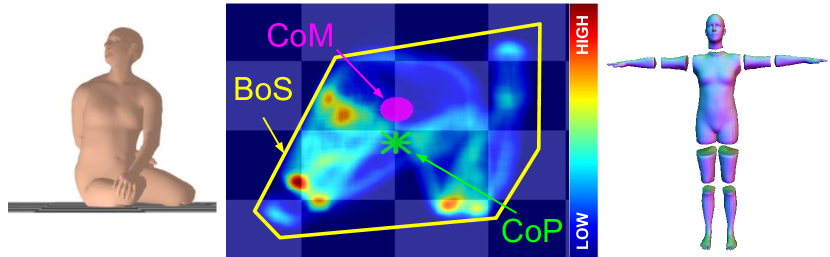
Figure 2: (1) A SMPL mesh sitting. (2) The inferred pressure map on the ground (color-coded heatmap), CoP (green), CoM (pink), and Base of Support (BoS, yellow polygon). (3) Segmentation of SMPL into $N_{P}=10$ parts, used for computing CoM; see Sec. 3.2.

The first involves computing CoM. To this end, we uniformly sample points on SMPL’s surface, and calculate each body part’s volume. Then, we compute CoM as the average of all uniformly sampled points weighted by the corresponding part volumes. We denote this as pCoM, standing for “part-weighted CoM”. Importantly, pCoM takes into account SMPL’s shape, pose, and all blend shapes, while it is also computationally efficient and differentiable.

The second involves estimating CoP directly from the image, without access to a pressure sensor. Our key insight is that the soft tissues of human bodies deform under pressure, e.g., the buttocks deform when sitting. However, SMPL does not model this deformation; it penetrates the ground instead of deforming. We use the penetration depth as a proxy for pressure [73]; deeper penetration means higher pressure. With this, we estimate a pressure field on SMPL’s mesh and compute the CoP as the pressure-weighted average of the surface points. Again this is differentiable.

For evaluation, we use a standard HPS benchmark (Human3.6M [37]), but also the RICH [35] dataset. However, these datasets have limited interactions with the floor. We thus capture a novel dataset, MoYo, of challenging yoga poses, with synchronized multi-view video, ground-truth SMPL-X [68] meshes, pressure sensor measurements, and body CoM. IPMAN, in both of its forms, and across all datasets, produces more accurate and stable 3D bodies than the state of the art. Importantly, we find that IPMAN improves accuracy for static poses, while not hurting dynamic ones. This makes IPMAN applicable to everyday motions.

To summarize: (1) We develop IPMAN, the first HPS method that integrates intuitive physics. (2) We infer biomechanical properties such as CoM, CoP and body pressure. (3) We define novel intuitive-physics terms that can be easily integrated into HPS methods. (4) We create MoYo, a dataset that uniquely has complex poses, multi-view video, and ground-truth bodies, pressure, and CoM. (5) We show that our IP terms improve HPS accuracy and physical plausibility. (6) Data and code are available for research.

2 Related Work

3D Human Pose and Shape (HPS) from images. Existing methods fall into two major categories: (1) non-parametric methods that reconstruct a free-form body representation, e.g., joints [1, 61, 62] or vertices [54, 63, 108], and (2) parametric methods that use statistical body models [25, 5, 42, 56, 68, 99, 105]. The latter methods focus on various aspects, such as expressiveness [13, 18, 68, 74, 94], clothed bodies [15, 95, 98], videos [24, 46, 83, 107], and multi-person scenarios [38, 80, 111], to name a few.

Inference is done by either optimization or regression. Optimization-based methods [7, 16, 68, 94, 95] fit a body model to image evidence, such as joints [11], dense vertex correspondences [2] or 2D segmentation masks [23]. Regression-based methods [43, 53, 50, 81, 110, 45, 117, 114] use a loss similar to the objective function of optimization methods to train a network to infer body model parameters. Several methods combine optimization and regression in a training loop [49, 64, 52]. Recent methods [41, 24] fine-tune pre-trained networks at test time w.r.t. an image or a sequence, retaining flexibility (optimization) while being less sensitive to initialization (regression).

Despite their success, these methods reason about the human in “isolation”, without taking the surrounding scene into account; see [82, 115] for a comprehensive review.

Contact-only scene constraints. A common way of using scene information is to consider body-scene contact [27, 28, 70, 91, 106, 112, 113, 118, 97, 101, 17, 12]. Yamamoto et al. [100] and others [27, 106, 112, 19, 75] ensure that estimated bodies have plausible scene contact. For videos, encouraging foot-ground contact reduces foot skating [36, 70, 77, 113, 118]. Weng et al. [91] use contact in estimating the pose and scale of scene objects, while Villegas et al. [87] preserve self- and ground contact for motion retargeting.

These methods typically take two steps: (1) detecting contact areas on the body and/or scene and (2) minimizing the distance between these. Surfaces are typically assumed to be in contact if their distance is below a threshold and their relative motion is small [27, 35, 106, 112].

Many methods only consider contact between the ground and the foot joints [118, 71] or other end-effectors [70]. In contrast, IPMAN uses the full 3D body surface and exploits this to compute the pressure, CoP and CoM. Unlike binary contact, this is differentiable, making the IP terms useful for training HPS regressors.

Physics-based scene constraints. Early work uses physics to estimate walking [9, 8] or full body motion [89]. Recent methods [71, 79, 78, 104, 96, 22, 21] regress 3D humans and then refine them through physics-based optimization. Physics is used for two primary reasons: (1) to regularise dynamics, reducing jitter [71, 79, 104, 51], and (2) to discourage interpenetration and encourage contact. Since contact events are discontinuous, the pipeline is either not end-to-end trainable or trained with reinforcement learning [69, 104]. Xie et al. [96] propose differentiable physics-inspired objectives based on a soft contact penalty, while DiffPhy [21] uses a differentiable physics simulator [31] during inference. Both methods apply the objectives in an optimization scheme, while IPMAN is applied to both optimization and regression. PhysCap [79] considers a pose as balanced, when the CoM is projected within the BoS. Rempe et al. [71] impose PD control on the pelvis, which they treat as a CoM. Scott et al. [76] regress foot pressure from 2D and 3D joints for stability analysis but do not use it to improve HPS.

All these methods use unrealistic bodies based on shape primitives. Some require known body dimensions [71, 79, 104] while others estimate body scale [96, 51]. In contrast, IPMAN computes CoM, CoP and BoS directly from the SMPL mesh. Clever et al. [14] and Luo et al. [58] estimate 3D body pose but from pressure measurements, not from images. Their task is fundamentally different from ours.

3 Method

3.1 Preliminaries

Given a color image, $\mathbf{I}$, we estimate the parameters of the camera and the SMPL body model [56].

Body model. SMPL maps pose, $\bm{\theta}$, and shape, $\bm{\beta}$, parameters to a 3D mesh, $\bm{M}(\bm{\theta},\bm{\beta})$. The pose parameters, $\bm{\theta}\in\mathbb{R}^{24\times 6}$, are rotations of SMPL’s 24 joints in a 6D representation [116]. The shape parameters, $\bm{\beta}\in\mathbb{R}^{10}$, are the first 10 PCA coefficients of SMPL’s shape space. The generated mesh $\bm{M}(\bm{\theta},\bm{\beta})$ consists of $N_{V}=6890$ vertices, $\bm{{V}}\in\mathbb{R}^{N_{V}\times 3}$, and $N_{F}=13776$ faces, $\bm{{F}}\in\mathbb{R}^{N_{F}\times 3\times 3}$.

Note that our regression method (IPMAN-R, Sec. 3.4.1) uses SMPL, while our optimization method (IPMAN-O, Sec. 3.4.2) uses SMPL-X [68], to match the models used by the baselines. For simplicity of exposition, we refer to both models as SMPL when the distinction is not important.

Camera. For the regression-based IPMAN-R, we follow the standard convention [43, 44, 49] and use a weak perspective camera with a 2D scale, $s$, translation, $\mathbf{t}^{c}=(t_{x}^{c},t_{y}^{c})$, fixed camera rotation, $\mathbf{R}^{c}=\bm{{I}}_{3}$, and a fixed focal length $(f_{x},f_{y})$. The root-relative body orientation $\mathbf{R}^{b}$ is predicted by the neural network, but body translation stays fixed at $\mathbf{t}^{b}=\mathbf{0}$ as it is absorbed into the camera’s translation.

For the optimization-based IPMAN-O, we follow Müller et al. [64] to use the full-perspective camera model and optimize the focal lengths $(f_{x},f_{y})$, camera rotation $\mathbf{R}^{c}$ and camera translation $\mathbf{t}^{c}$. The principal point $(o_{x},o_{y})$ is the center of the input image. $\mathbf{K}$ is the intrinsic matrix storing focal lengths and the principal point. We assume that the body rotation $\mathbf{R}^{b}$ and translation $\mathbf{t}^{b}$ are absorbed into the camera parameters, thus, they stay fixed as $\mathbf{R}^{b}=\bm{{I}}_{3}$ and $\mathbf{t}^{b}=\mathbf{0}$. Using the camera, we project a 3D point $\mathbf{X}\in\mathbb{R}^{3}$ to an image point $\mathbf{x}\in\mathbb{R}^{2}$ through $\mathbf{x}=\mathbf{K}(\mathbf{R}^{c}\mathbf{X}+\mathbf{t}^{c})$.

Ground plane and gravity-projection. We assume that the gravity direction is perpendicular to the ground plane in the world coordinate system. Thus, for any arbitrary point in 3D space, $\bm{{u}}\in\mathbb{R}^{3}$, its gravity-projected point, $\bm{{u^{\prime}}}=g(\bm{{u}})\in\mathbb{R}^{3}$, is the projection of $\bm{{u}}$ along the plane normal $\bm{{n}}$ onto the ground plane, and $g(.)$ is the projection operator. The function $h(\bm{{u}})$ returns the signed “height” of a point $\bm{{u}}$ with respect to the ground; i.e., the signed distance from $\bm{{u}}$ to the ground plane along the gravity direction, where $h(\bm{{u}})<0$ if $\bm{{u}}$ is below the ground and $h(\bm{{u}})>0$ if $\bm{{u}}$ is above it.

3.2 Stability Analysis

We follow the biomechanics literature [32, 33, 66] and Scott et al. [76] to define three fundamental elements for stability analysis: We use the Newtonian definition for the “Center of Mass” (CoM); i.e., the mass-weighted average of particle positions. The “Center of Pressure” (CoP) is the ground-reaction force’s point of application. The “Base of Support” (BoS) is the convex hull of all body-ground contacts. Below, we define intuitive-physics (IP) terms using the inferred CoM and CoP. BoS is only used for evaluation.

Body Center of Mass (CoM). We introduce a novel CoM formulation that is fully differentiable and considers the per-part mass contributions, dubbed as pCoM; see Sup. Mat. for alternative CoM definitions. To compute this, we first segment the template mesh into $N_{P}=10$ parts $P_{i}\in\mathcal{P}$; see Fig. 2. We do this once offline, and keep the segmentation fixed during training and optimization. Assuming a shaped and posed SMPL body, the per-part volumes $\mathcal{V}^{P_{i}}$ are calculated by splitting the SMPL mesh into parts.

However, mesh splitting is a non-differentiable operation. Thus, it cannot be used for either training a regressor (IPMAN-R) or for optimization (IPMAN-O). Instead, we work with the full SMPL mesh and use differentiable “close-translate-fill” operations for each body part on the fly. First, for each part $P$, we extract boundary vertices $\mathcal{B}_{P}$ and add in the middle a virtual vertex $\bm{{v}}_{g}$, where $\bm{{v}}_{g}=\sum_{j\in\mathcal{B}_{P}}\bm{{v}}_{j}/|\mathcal{B}_{P}|$. Then, for the $\mathcal{B}_{P}$ and $\bm{{v}}_{g}$ vertices, we add virtual faces to “close” $P$ and make it watertight. Next, we “translate” $P$ such that the part centroid $\mathbf{c}_{P}=\sum_{j\in P}\bm{{v}}_{j}/|P|$ is at the origin. Finally, we “fill” the centered $P$ with tetrahedrons by connecting the origin with each face vertex. Then, the part volume, $\mathcal{V}^{\mathcal{P}}$, is the sum of all tetrahedron volumes [109].

To create a uniform distribution of surface vertices, we uniformly sample $N_{U}=20000$ surface points $\bm{{V}}_{U}\in\mathbb{R}^{N_{U}\times 3}$ on the template SMPL mesh using the Triangle Point Picking method [90]. Given $\bm{{V}}_{U}$ and the template SMPL mesh vertices $\bm{{V}}_{T}$, we follow [64], and analytically compute a sparse linear regressor $\mathbf{W}\in\mathbb{R}^{N_{U}\times N_{V}}$ such that $\bm{{V}}_{U}=\mathbf{W}\bm{{V}}_{T}$. During training and optimization, given an arbitrary shaped and posed mesh with vertices $\bm{{V}}$, we obtain uniformly-sampled mesh surface points as $\bm{{V}}_{U}=\mathbf{W}\bm{{V}}$. Each surface point, $v_{i}$, is assigned to the body part, $P_{v_{i}}$, corresponding to the face, $\bm{{F}}_{v_{i}}$, it was sampled from.

Finally, the part-weighted pCoM is computed as a volume-weighted mean of the mesh surface points:

$$\bar{\mathbf{m}}=\frac{\sum_{i=1}^{N_{U}}\mathcal{V}^{P_{v_{i}}}v_{i}}{\sum_{i=1}^{N_{U}}\mathcal{V}^{P_{v_{i}}}}\text{,}$$ (1)

where $\mathcal{V}^{P_{v_{i}}}$ is the volume of the part $P_{v_{i}}\in\mathcal{P}$ to which $v_{i}$ is assigned. This formulation is fully differentiable and can be employed with any existing 3D HPS estimation method.

Note that computing CoM (or volume) from uniformly sampled surface points does not work (see Sup. Mat.) because it assumes that mass, $M$, is proportional to surface area, $S$. Instead, our pCoM computes mass from volume, $\mathcal{V}$, via the standard density equation, $M=\rho\mathcal{V}$, while our close-translate-fill operation computes the volume of deformable bodies in an efficient and differentiable manner.

Center of Pressure (CoP). Recovering a pressure heatmap from an image without using hardware, such as pressure sensors, is a highly ill-posed problem. However, stability analysis requires knowledge of the pressure exerted on the human body by the supporting surfaces, like the ground. Going beyond binary contact, Rogez et al. [73] estimate 3D forces by detecting intersecting vertices between hand and object meshes. Clever et al. [14] recover pressure maps by allowing articulated body models to deform a soft pressure-sensing virtual mattress in a physics simulation.

In contrast, we observe that, while real bodies interacting with rigid objects (e.g., the floor) deform under contact, SMPL does not model such soft-tissue deformations. Thus, the body mesh penetrates the contacting object surface and the amount of penetration can be a proxy for pressure; a deeper penetration implies higher pressure. With the height $h(v_{i})$ (see Sec. 3.1) of a mesh surface point $v_{i}$ with respect to the ground plane $\Pi$, we define a pressure field to compute the per-point pressure $\rho_{i}$ as:

$$\rho_{i} = \begin{cases}1-\alpha h(v_{i})&\text{if~{}}h(v_{i})<0\text{,}\\ e^{-\gamma h(v_{i})}&\text{if~{}}h(v_{i})\geq 0\text{,}\end{cases}$$ (2)

where $\alpha$ and $\gamma$ are scalar hyperparameters set empirically. We approximate soft tissue via a “spring” model and “penetrating” pressure field using Hooke’s Law. Some pressure is also assigned to points above the ground to allow tolerance for footwear, but this decays quickly. Finally, we compute the CoP, $\mathbf{\bar{s}}$, as

$$\mathbf{\bar{s}} = \frac{\sum_{i=1}^{N_{U}}\rho_{i}v_{i}}{\sum_{i=1}^{N_{U}}\rho_{i}}\text{.}$$ (3)

Again, note that this term is fully differentiable.

Base of Support (BoS). In biomechanics [34, 92], BoS is defined as the “supporting area” or the possible range of the CoP on the supporting surface. Here, we define BoS as the convex hull [72] of all gravity-projected body-ground contact points. In detail, we first determine all such contacts by selecting the set of mesh surface points $v_{i}$ close to the ground, and then gravity-project them onto the ground to obtain $C=\{g(v_{i})\;\bigr{|}\;|h(v_{i})|<\tau\}$. The BoS is then defined as the convex hull $\mathcal{C}$ of $C$.

3.3 Intuitive-Physics Losses

Stability loss. The “inverted pendulum” model of human balance [92, 93] considers the relationship between the CoM and BoS to determine stability. Simply put, for a given shape and pose, if the body CoM, projected on the gravity-aligned ground plane, lies within the BoS, the pose is considered stable. While this definition of stability is useful for evaluation, using it in a loss or energy function for 3D HPS estimation results in sparse gradients (see Sup. Mat.). Instead, we define the stability criterion as:

$$\mathcal{L}_{\text{stability}} = \|g(\bar{\mathbf{m}})\;-\;g(\bar{\mathbf{s}})\|_{2}\text{,}$$ (4)

where $g(\bar{\mathbf{m}})$ and $g(\bar{\mathbf{s}})$ are the gravity-projected CoM and CoP, respectively.

Ground contact loss. As shown in Fig. 1, 3D HPS methods minimize the 2D joint reprojection error and do not consider the plausibility of body-ground contact. Ignoring this can result in interpenetrating or hovering meshes. Inspired by self-contact losses [19, 64] and hand-object contact losses [26, 29], we define two ground losses, namely pushing, $\mathcal{L}_{\text{push}}$, and pulling, $\mathcal{L}_{\text{pull}}$, that take into account the height, $h(v_{i})$, of a vertex, $v_{i}$, with respect to the ground plane. For $h(v_{i})<0$, i.e., for vertices under the ground plane, $\mathcal{L}_{\text{push}}$ discourages body-ground penetrations. For $h(v_{i})\geq 0$, i.e., for hovering meshes, $\mathcal{L}_{\text{pull}}$ encourages the vertices that lie close to the ground to “snap” into contact with it. Note that the losses are non-conflicting as they act on disjoint sets of vertices. Then, the ground contact loss is:

$$\mathcal{L}_{\text{ground}} = \mathcal{L}_{\text{pull}}+\mathcal{L}_{\text{push}}\text{, with }$$ (5)

$$\mathcal{L}_{\text{pull}} = \alpha_{1}\tanh{(\frac{h(v_{i})}{\alpha_{2}})^{2}}\quad\text{if~{}}h(v_{i})\geq 0\text{, and }$$ (6)

$$\mathcal{L}_{\text{push}} = \beta_{1}\tanh{(\frac{h(v_{i})}{\beta_{2}})^{2}}\quad\text{if~{}}h(v_{i})<0\text{.}$$ (7)

3.4 IPMAN

We use our new IP losses for two tasks: (1) We extend HMR [43] to develop IPMAN-R, a regression-based HPS method. (2) We extend SMPLify-XMC [64] to develop IPMAN-O, an optimization-based method. Note that IPMAN-O uses a reference ground plane, while IPMAN-R uses the ground plane only for training but not at test time. It leverages the known ground in 3D datasets, and thus, does not require additional data beyond past HPS methods.

3.4.1 IPMAN-R

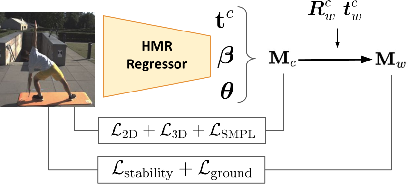
Figure 3: IPMAN-R architecture. First, the HMR regressor estimates camera translation and SMPL parameters for an input image. These parameters are used to generate the SMPL mesh in the camera frame, $\bm{{M}}_{c}$. To transform the mesh from camera into world coordinates ($\bm{{M}}_{c}\rightarrow\bm{{M}}_{w}$), IPMAN-R uses the ground-truth camera rotation, $\bm{{R}}^{c}_{w}$, and translation, $\bm{{t}}^{c}_{w}$. The IP losses, $\mathcal{L}_{\text{ground}}$ and $\mathcal{L}_{\text{stability}}$, are applied on the mesh in the world coordinate system.

Most HPS methods are trained with a mix of direct supervision using 3D datasets [37, 61, 88] and 2D reprojection losses using image datasets [55, 39, 4]. The 3D losses, however, are calculated in the camera frame, ignoring scene information and physics. IPMAN-R extends HMR [43] with our intuitive-physics terms; see Fig. 3 for the architecture. For training, we use the known camera coordinates and the world ground plane in 3D datasets.

As described in Sec. 3.1 (paragraph “Camera”), HMR infers the camera translation, $\mathbf{t}^{c}$, and SMPL parameters, $\bm{\theta}$ and $\bm{\beta}$, in the camera coordinates assuming $\mathbf{R}^{c}=\bm{{I}}_{3}$ and $\mathbf{t}^{b}=\mathbf{0}$. Ground truth 3D joints and SMPL parameters are used to supervise the inferred mesh $\bm{{M}}_{c}$ in the camera frame. However, 3D datasets also provide the ground, albeit in the world frame. To leverage the known ground, we transform the predicted body orientation, $\mathbf{R}^{b}$, to world coordinates using the ground-truth camera rotation, $\mathbf{R}^{c}_{w}$, as $\mathbf{R}^{b}_{w}=\mathbf{R}^{c\top}_{w}\mathbf{R}^{b}$. Then, we compute the body translation in world coordinates as $\mathbf{t}^{b}_{w}=-\mathbf{t}^{c}+\mathbf{t}^{c}_{w}$. With the predicted mesh and ground plane in world coordinates, we add the IP terms, $\mathcal{L}_{\text{stability}}$ and $\mathcal{L}_{\text{ground}}$, for HPS training as follows:

$$\mathcal{L}_{\text{{\color[rgb]{0,0,0}\mbox{IPMAN-R}}}}(\bm{{\theta}},\bm{{\beta}},\mathbf{t}^{c})= \lambda_{{2D}}\mathcal{L}_{{2D}}+\lambda_{{3D}}\mathcal{L}_{{3D}}+\lambda_{\text{SMPL}}\mathcal{L_{\text{SMPL}}}+$$

$$\lambda_{\text{s}}\mathcal{L}_{\text{stability}}+\lambda_{\text{g}}\mathcal{L}_{\text{ground}}\text{,}$$ (8)

where $\lambda_{\text{s}}$ and $\lambda_{\text{g}}$ are the weights for the respective IP terms. For training (data augmentation, hyperparameters, etc), we follow Kolotouros et al. [49]; for more details see Sup. Mat.

3.4.2 IPMAN-O

To fit SMPL-X to 2D image keypoints, SMPLify-XMC [64] initializes the fitting process by exploiting the self-contact and global-orientation of a known/presented 3D mesh. We posit that the presented pose contains further information, such as stability, pressure and contact with the ground-plane. IPMAN-O uses this insight to apply stability and ground contact losses. The IPMAN-O objective is:

$$E_{\text{{\color[rgb]{0,0,0}\mbox{IPMAN-O}}}}(\bm{{\beta}},\bm{{\theta}},\bm{{\Phi}})= E_{J2D}+\lambda_{\beta}E_{\beta}+\lambda_{\theta_{h}}E_{\theta_{h}}+$$

$$\lambda_{\tilde{\theta_{b}}}E_{\tilde{\theta_{b}}}+\lambda_{\tilde{C}}E_{\tilde{C}}+$$

$$\lambda_{s}E_{\text{stability}}+\lambda_{g}E_{\text{ground}}\text{.}$$ (9)

$\bm{{\Phi}}$ denotes the camera parameters: rotation $\mathbf{R}^{c}$, translation $\mathbf{t}^{c}$, and focal length, $(f_{x},f_{y})$. $E_{J2D}$ is a 2D joint loss, $E_{\beta}$ and $E_{\theta_{h}}$ are $L_{2}$ body shape and hand pose priors. $E_{\tilde{\theta_{b}}}$ and $E_{\tilde{C}}$ are pose and contact terms w.r.t. the presented 3D pose and contact (see [64] for details). $E_{S}$ and $E_{G}$ are the stability and ground contact losses from Sec. 3.3. Since the estimated mesh is in the same coordinate system as the presented mesh and the ground-plane, we directly apply IP losses without any transformations. For details see Sup. Mat.

4 Experiments

4.1 Training and Evaluation Datasets

Human3.6M [37]. A dataset of 3D human keypoints and RGB images. The poses are limited in terms of challenging physics, focusing on common activities like walking, discussing, smoking, or taking photos.

RICH [35]. A dataset of videos with accurate marker-less motion-captured 3D bodies and 3D scans of scenes. The images are more natural than Human3.6M and Fit3D [20]. We consider sequences with meaningful body-ground interaction. For the list of sequences, see Sup. Mat.

Other datasets. Similar to [49], for training we use 3D keypoints from MPI-INF-3DHP [61] and 2D keypoints from image datasets such as COCO [55], MPII [4] and LSP [39].

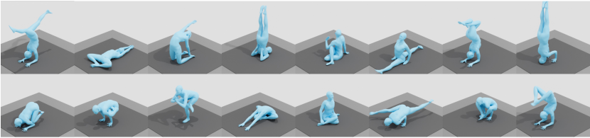
Figure 4: Representative examples illustrating the variation and complexity of 3D pose and body-ground contact in our new MoYo dataset.

4.1.1 MoCap Yoga (MoYo) Dataset

We capture a trained Yoga professional in 200 highly complex poses (see Fig. 4) using a synchronized MoCap system, pressure mat, and a multi-view RGB video system with 8 static, calibrated cameras; for details see Sup. Mat. The dataset contains $\sim 1.75$M RGB frames in 4K resolution with ground-truth SMPL-X [68], pressure and CoM. Compared to the Fit3D [20] and PosePrior [1] datasets, MoYo is more challenging; it has extreme poses, strong self-occlusion, and significant body-ground and self-contact.

4.2 Evaluation Metrics

We use standard 3D HPS metrics: The Mean Per-Joint Position Error (MPJPE), its Procrustes Aligned version (PA-MPJPE), and the Per-Vertex Error (PVE) [67].

BoS Error (BoSE). To evaluate stability, we propose a new metric called BoS Error (BoSE). Following the definition of stability (Eq. 4) we define:

BoSE $$= \begin{cases}1&g(\bar{\mathbf{m}})\in\mathcal{C}(C)\\ 0&g(\bar{\mathbf{m}})\notin\mathcal{C}(C)\\ \end{cases}$$ (10)

where $\mathcal{C}(C)$ is the convex hull of the gravity-projected contact vertices for $\tau=10$ cm. For efficiency reasons, we formulate this computation as the solution of a convex system via interior point linear programming [3]; see Sup. Mat.

4.3 IPMAN Evaluation

IPMAN-R. We evaluate our regressor, IPMAN-R, on RICH and H3.6M and summarize our results in Tab. 1. We refer to our regression baseline as $\text{\mbox{HMR}}^{*}$ which is HMR trained on the same datasets as IPMAN-R. Since we train with paired 3D datasets, we do not use HMR’s discriminator during training. Both IP terms individually improve upon the baseline method. Their joint use, however, shows the largest improvement. For example, on RICH the MPJPE improves by 3.5mm and the PVE by 2.5mm. It is particularly interesting that IPMAN-R improves upon the baseline on H3.6M, a dataset with largely dynamic poses and little body-ground contact. We also significantly outperform ($\sim 12\%$) the MPJPE of optimization approaches that use the ground plane, Zou et al. [118] (69.9 mm) and Zanfir et al. [106] (69.0 mm), on H3.6M. Some video-based methods  [104, 51] achieve better MPJPE ($56.7$ and $52.5$ resp.) on H3.6M. However, they initialize with a stronger kinematic predictor [46, 52] and require video frames as input. Further, they use heuristics to estimate body weight and non-physical residual forces to correct for contact estimation errors. In contrast, IPMAN is a single-frame method, models complex full-body pressure and does not rely on approximate body weight to compute CoM. Qualitatively, Fig. 5 (top) shows that IPMAN-R’s reconstructions are more stable and contain physically-plausible body-ground contact. While HMR is not SOTA, it is simple, isolating the benefits of our new IP formulation. These terms can also be added to methods with more modern backbones and architectures.

  Method RICH Human3.6M MPJPE $\downarrow$ PAMPJPE $\downarrow$ PVE $\downarrow$ BoSE (%) $\uparrow$ MPJPE $\downarrow$ PAMPJPE $\downarrow$ PhysCap [79] - - - - 113.0 68.9 DiffPhy [21] - - - - 81.7 55.6 Zou et al. [118] - - - - 69.9 - Xie et al. [96] - - - - 68.1 - VIBE [46] - - - - 61.3 43.1 Simpoe [104] - - - - 56.7 41.6 D&D [51] - - - - 52.5 35.5 HMR [43] - - - - 88.0 56.8 Zanfir et al. [106] - - - - 69.0 - SPIN [49] 112.2 71.5 129.5 54.7 62.3 41.9 PARE [47] 107.0 73.1 125.0 74.4 - - CLIFF [53] 107.0 67.2 122.3 67.6 81.4 52.1 Finetuning on Human3.6M $\text{\mbox{HMR}}^{*}$ [43] - - - - 62.1 41.6 IPMAN-R (Ours) - - - - 60.7 (-1.4) 41.1 (-0.5) Finetuning on all datasets $\text{\mbox{HMR}}^{*}$ [43] 82.5 48.3 92.4 62.0 61.6 41.9 $\text{\mbox{HMR}}^{*}$ [43]$+\mathcal{L}\text{ground}$ 80.9 47.8 89.9 66.5 61.9 41.8 $\text{\mbox{HMR}}^{*}$ [43]$+\mathcal{L}\text{stability}$ 81.0 47.5 (-0.8) 90.8 69.6 61.2 41.9 IPMAN-R (Ours) 79.0 (-3.5) 47.6 89.9 (-2.5) 71.2 (+9.2) 60.6 (-1.0) 41.8 (-0.1)  

Table 1: Top to Bottom: Comparisons with video-based and single-frame regression methods. IPMAN-R outperforms the single-frame baselines across all benchmarks. * indicates training hyperparameters and datasets are identical to IPMAN-R. All units are in mm except BoSE. Bold denotes best results (per category), and parentheses show improvement over the baseline.  Zoom in

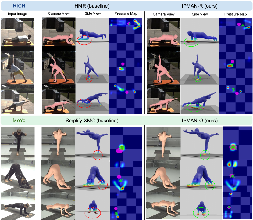
Figure 5: Qualitative evaluation of IPMAN-R and IPMAN-O on the RICH and MoYo datasets. The first column shows the input images of a subject doing various sports poses. The second and third block of columns show the baseline’s and our results, respectively. In each block, the first image shows the estimated mesh overlayed on the image (camera view), the second image shows the estimated mesh in the world frame (side view), and the last image shows the estimated pressure map with the CoM (in pink) and the CoP (in green).

IPMAN-O. Our optimization method, IPMAN-O, also improves upon the baseline optimization method, SMPLify-XMC, on all evaluation metrics (see Tab. 2). We note that adding $L_{\text{stability}}$ independently improves the PVE, but not joint metrics (PA-MPJPE, MPJPE) and BoSE. This can be explained by the dependence of our IP terms on the relative position of the mesh surface to the ground-plane. Since joint metrics do not capture surfaces, they may get worse. Similar trends on joint metrics have been reported in the context of hand-object contact [29, 84] and body-scene contact [27]. We show qualitative results in Fig. 5 (bottom). While both SMPLify-XMC [64] and IPMAN-O achieve similar image projections, another view reveals that our results are more stable and physically plausible w.r.t. the ground.

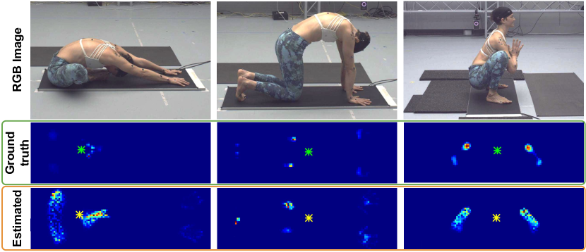
Figure 6: Qualitative comparison of estimated vs the ground-truth pressure. The ground-truth CoP is shown in green and the estimated CoP is shown in yellow. Pressure heatmap colors as per Fig. 2.

4.4 Pressure, CoP and CoM Evaluation

We evaluate our estimated pressure, CoP and CoM against the MoYo ground truth. For pressure evaluation, we measure Intersection-over-Union (IoU) between our estimated and ground-truth pressure heatmaps. We also compute the CoP error as the Euclidean distance between estimated and ground-truth CoP. We obtain an IoU of $0.32$ and a CoP error of $57.3$ mm. Figure 6 shows a qualitative visualization of the estimated pressure compared to the ground truth. For CoM evaluation, we find a $53.3$ mm difference between our pCoM and the CoM computed by the commercial software, Vicon Plug-in Gait. Unlike Vicon’s estimate, our pCoM does not require anthropometric measurements and takes into account the full 3D body shape. For details about the evaluation protocol and comparisons with alternative CoM formulations, see Sup. Mat.

Physics Simulation. To evaluate stability, we run a post-hoc physics simulation in “Bullet” [10] and measure the displacement of the estimated meshes; a small displacement denotes a stable pose. IPMAN-O produces $14.8\%$ more stable bodies than the baseline [64]; for details see Sup. Mat.

  Method MoYo MPJPE $\downarrow$ PAMPJPE $\downarrow$ PVE $\downarrow$ BoSE (%) $\uparrow$ SMPLify-XMC [64] 75.3 36.5 16.8 98.0 SMPLify-XMC [64]$+\mathcal{L}\text{ground}$ 73.3 36.2 14.5 98.2 SMPLify-XMC [64]$+\mathcal{L}\text{stability}$ 88.5 38.6 15.3 97.8 IPMAN-O (Ours) 71.9 (-3.4) 34.3 (-2.2) 11.4 (-5.4) 98.6 (+0.5)  

Table 2: Evaluation of IPMAN-O and SMPLify-XMC [64] (optimization-based) on MoYo. Bold shows the best performance, and parentheses show the improvement over SMPLify-XMC.

5 Conclusion

Existing 3D HPS estimation methods recover SMPL meshes that align well with the input image, but are often physically implausible. To address this, we propose IPMAN, which incorporates intuitive-physics in 3D HPS estimation. Our IP terms encourage stable poses, promote realistic floor support, and reduce body-floor penetration. The IP terms exploit the interaction between the body CoM, CoP, and BoS – key elements used in stability analysis. To calculate the CoM of SMPL meshes, IPMAN uses on a novel formulation that takes part-specific mass contributions into account. Additionally, IPMAN estimates proxy pressure maps directly from images, which is useful in computing CoP. IPMAN is simple, differentiable, and compatible with both regression and optimization methods. IPMAN goes beyond previous physics-based methods to reason about arbitrary full-body contact with the ground. We show that IPMAN improves both regression and optimization baselines across all metrics on existing datasets and MoYo. MoYo uniquely comprises synchronized multi-view video, SMPL-X bodies in complex poses, and measurements for pressure maps and body CoM. Qualitative results show the effectiveness of IPMAN in recovering physically plausible meshes.

While IPMAN addresses body-floor contact, future work should incorporate general body-scene contact and diverse supporting surfaces by integrating 3D scene reconstruction. In this work, the proposed IP terms are designed to help static poses and we show that they do not hurt dynamic poses. However, the large body of biomechanical literature analyzing dynamic poses could be leveraged for activities like walking, jogging, running, etc. It would be interesting to extend IPMAN beyond single-person scenarios by exploiting the various physical constraints offered by multiple subjects.

Acknowledgements. We thank T. Alexiadis, G. Becherini, T. McConnell, C. Gallatz, M. Höschle, S. Polikovsky, C. Mendoza, Y. Fincan, L. Sanchez and M. Safroshkin for the MoYo data, J. Tesch, N. Athanasiou, Z. Fang, V. Choutas and all of Perceiving Systems for fruitful discussions. This work is funded by the International Max Planck Research School for Intelligent Systems (IMPRS-IS) and in part by the German Federal Ministry of Education and Research (BMBF), Tübingen AI Center, FKZ: 01IS18039B.

Disclosure. https://files.is.tue.mpg.de/black/CoI_CVPR_2023.txt

Supplementary Material

Appendix A MoCap Yoga Dataset (MoYo)

We capture a trained yoga professional in a MoCap studio with 54 Vicon Vantage V16 infrared cameras capable of tracking body markers as small as 3mm in diameter. The Vicon system was synchronized with 8 RGB cameras recording at 4112x3008 resolution and a Zebris FDM pressure measurement mat. The pressure mat offers a sensor resolution of 1.4sensors/cm² and can capture pressure in 10-1200 kPa range. Ground-truth SMPL-X [68] parameters are recovered from the MoCap data using MoSh++ [59]. A total of 200 yoga sequences were recorded at 30fps. The yoga poses we selected include all poses in the Yoga-82 dataset [86] as well as their variations. The T-SNE [85] plot in Fig. S.1 shows that the poses contained in MoYo are highly diverse and cover areas in the space of human poses not well represented in existing datasets [37, 59, 61, 67].

To compute a reference CoM, we use the commercially available tool, Plug-in Gait (PiG) from Vicon. PiG requires a-priori known anthropometric measurements (e.g. height, weight, shoulder offset, knee width, etc) and computes: (1) bone joints from a known marker topology, (2) per-bone mass as a proportion of body mass, (3) per-bone CoM as a proportion of each bone’s length, and (4) whole-body CoM as a weighted average of per-bone CoMs. In contrast, our pCoM does not require anthropometric measurements and takes into account the full 3D body shape.

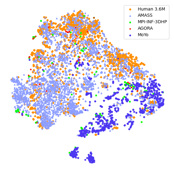
Figure S.1: The distribution of poses in MoYo and existing MoCap datasets are visualized after T-SNE dimension reduction.

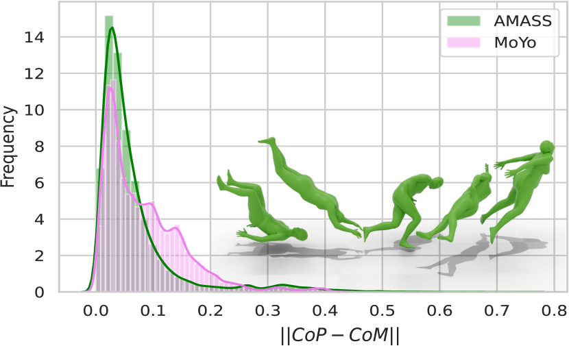
Figure S.2: Distribution of $\mathcal{L}_{\text{stability}}$ in AMASS and MoYo. Both peak at $\sim 0$, motivating using an $L_{2}$ formulation. Bottom right: Unstable long-tail poses from AMASS.

Appendix B Method

B.1 Stability Loss

The suggested classic definition uses a binary stability criterion, i.e., the CoM “just” projects either inside or outside the BoS. This is discontinuous with sparse gradients.

Since CoP lies inside BoS, our L2 loss is a “soft” version that approximates the classic definition, but has two key benefits: (1) it is continuous and fully differentiable, and, (2) it informs about the degree of instability. The distribution of $\mathcal{L}_{\text{stability}}$ in Fig. S.2 for both AMASS and MoYo datasets peak at $\sim 0$, motivating using an $L_{2}$ formulation.

B.2 Elements of Stability Analysis: Alternative formulations

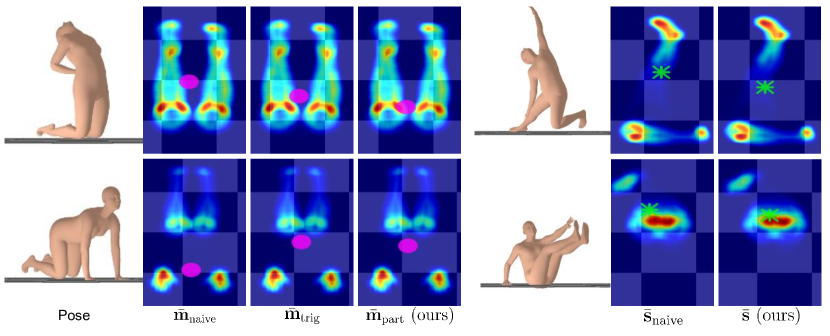
Figure S.3: Gravity-projections of different formulations of CoM (shown with pink) and CoP (shown with green) are shown with estimated pressure maps. Our proposed pCoM captures more accurate body mass distribution because it takes into account part-specific mass contributions. Similarly, our CoP leverages the pressure maps rather than binary contact.

Computation of the “Center of Mass”, CoM, must be efficient and differentiable. The CoM could be naively approximated as the mean vertex position of a mesh:

$$\bar{\mathbf{m}}_{\text{naive}}=\frac{1}{N_{V}}\sum_{i=1}^{N_{V}}\bm{{v}}_{i}\text{.}$$ (S.1)

However, the SMPL and the SMPL-X body models have a non-uniform vertex distribution across the surface. There are a disproportionate number of vertices on the face and hands compared to the body. For instance, roughly half of SMPL-X’s vertices lie on the head. Consequently, $\bar{\mathbf{m}}_{\text{naive}}$ is dominated by face and hand vertices.

A better formulation is the mean of uniformly sampled surface points:

$$\bar{\mathbf{m}}^{u}_{\text{naive}}=\frac{1}{N_{U}}\sum_{i=1}^{N_{U}}\bm{{v}}_{i}\text{.}$$ (S.2)

Another formulation computes the average of the mesh triangle face centroids weighted by the face area:

$$\bar{\mathbf{m}}_{\text{trig}}=\frac{\sum_{i=1}^{N_{F}}A_{i}\bar{F_{i}}}{\sum_{i=1}^{N_{F}}A_{i}}\text{,}$$ (S.3)

where $A_{i}$ denotes the area and $\bar{F_{i}}=\frac{1}{3}(\bm{{v}}_{i_{1}}^{\top}+\bm{{v}}_{i_{2}}^{\top}+\bm{{v}}_{i_{3}}^{\top})$ the centroid of face $\bm{{F}}_{i}$. The problem with these approaches is that they assume that mass, $M$, is proportional to surface area, $S$, which is a poor approximation.

Our proposed pCoM formulation addresses this by $(1)$ uniformly sampling vertices on the SMPL mesh and $(2)$ taking part-specific mass contributions into account. Our pCoM computes mass from volume, $\mathcal{V}$, via the standard density equation, $M=\rho\mathcal{V}$. Tab. S.1 compares the CoM error across different formulations of CoM w.r.t. ground-truth CoM obtained using Vicon PiG. pCoM significantly outperforms all baselines. Figure S.3 shows an intuitive qualitative comparison between all formulations of CoM.

  $\bar{\mathbf{m}}_{\text{naive}}$ $\bar{\mathbf{m}}^{u}_{\text{naive}}$ $\bar{\mathbf{m}}_{\text{trig}}$ pCoM ($\bar{m}$) CoM error $\downarrow$ 264.1 mm 68.5 mm 70.0 mm 53.3 mm  

Table S.1: Comparison of various CoM formulations.

Similarly, for “Center of Pressure” (CoP), a simple heuristic used in previous works detects binary contact by thresholding body vertices using their Euclidean distance from the ground plane. However, such contact lacks information about the pressure distribution and assigns equal weight to all contact vertices. Moreover, binary contact is not differentiable and is therefore generally used at test-time [27, 87, 106, 112] or for data preprocessing [28, 113], not during training. In contrast, our CoP formulation is fully differentiable and takes the inferred pressure distribution of the body-floor contact into account. As shown in Fig. S.3, the naive CoP suffers from equally weighting all binary-contact whereas our CoP better represents the pressure profile of the body-ground contact.

B.3 Ablation of ground losses

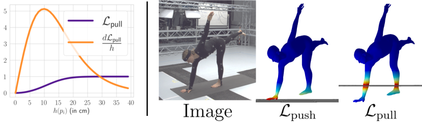
Figure S.4: Left: The gradient of $\mathcal{L}_{\text{pull}}$ decays gradually with $h(p_{i})$; vertices with $h(p_{i})\geq 20$cm contribute minimally to back-propagation. Right: Effect of $\mathcal{L}_{\text{push}}$ and $\mathcal{L}_{\text{pull}}$; high $\mathcal{L}_{\text{push}}$ results in inaccurate floor contact, high $\mathcal{L}_{\text{pull}}$ results in penetrations.

Instead of having a threshold to restrict $\mathcal{L}_{\text{pull}}$ only to vertices close to the ground, we chose a soft version of the loss to ensure full differentiability. However, as shown in Fig. S.4 (left), the loss gradient decays with height and vertices with $h(v_{i})\geq 15$ cm contribute minimally during back-propagation. Further, we study the impact of $\mathcal{L}_{\text{push}}$ and $\mathcal{L}_{\text{pull}}$ in Tab. S.2 and Fig. S.4-right. The terms complement each other and are more effective when used jointly ($\mathcal{L}_{\text{ground}}$).

Method	MPJPE $\downarrow$	PMPJPE $\downarrow$	PVE $\downarrow$
$\text{\mbox{HMR}}^{*}$ [43]	82.5	48.2	92.3
$\text{\mbox{HMR}}^{*}$ [43]$+\mathcal{L}_{\text{push}}$	85.4	49.0	96.6
$\text{\mbox{HMR}}^{*}$ [43]$+\mathcal{L}_{\text{pull}}$	88.0	48.8	99.4
$\text{\mbox{HMR}}^{*}$ [43]$+\mathcal{L}_{\text{ground}}$	80.9	47.8	89.9

Table S.2: Ablation for $\mathcal{L}_{\text{push}}$ and $\mathcal{L}_{\text{pull}}$ on the RICH [35] dataset.

Appendix C Experiments

We integrate our intuitive-physics terms in both an optimization- and a regression-based method for three reasons: (1) the community heavily uses both method types, (2) our terms generalize and benefit both types, despite their differences, and (3) our terms also work with different body models; SMPL-X (used by IPMAN-O) and SMPL (used by IPMAN-R).

C.1 IPMAN Implementation Details

C.1.1 IPMAN-R.

Similar to previous methods [48, 49, 64, 38], we take the widely used HMR [43] architecture to analyze the effect of adding our proposed IP terms. Note that, while HMR is not the most recent method, it is widely used as a backbone. As such, it provides a consistent foundation for evaluation and comparison. Our goal here is to isolate and evaluate the effect of adding intuitive physics. Such terms should then be readily applicable to other HPS regression frameworks.

The HMR regressor estimates the camera translation $\mathbf{t}^{c}$ and SMPL parameters (pose, global orientation, and shape) in the camera coordinates assuming $\mathbf{R}^{c}=\bm{{I}}_{3}$ and $\mathbf{t}^{b}=\mathbf{0}$. We initialize the HMR model using pretrained weights provided by SPIN [49] and finetune both IPMAN-R and HMR on the same datasets; namely RICH [35], Human3.6M [37], MPI-INF-3DHP [61], COCO [55], MPII [4] and LSP [39, 40]. In the main paper, we call the baseline as $\text{\mbox{HMR}}^{*}$ which uses the same training datasets and hyperparameters as IPMAN-R, albeit with the exception of the proposed IP terms. We follow the same training schedule, data augmentation and hyperparameters as SPIN [49] but do not use in-the-loop optimization. We use the Adam optimizer with learning rate of $5e^{-5}$ and finetuning takes 3 epochs ($\sim 8$ hours) on a Nvidia Tesla V100 GPU.

We set the hyperparameters $\alpha=100$, $\gamma=10$ for the per-vertex pressure $\rho_{i}$, $\alpha_{1}=1.0$, $\alpha_{2}=0.15$ for the $\mathcal{L}_{\text{pull}}$ term and $\beta_{1}=10.0$, $\beta_{2}=0.15$ for the $\mathcal{L}_{\text{push}}$ term. The loss weights are empirically determined to be $\lambda_{s}=0.01$ and $\lambda_{g}=0.01$. We borrow the same configuration as [49] for all remaining loss weights, namely $\mathcal{\lambda}_{\text{2D}}$, $\mathcal{\lambda}_{\text{3D}}$ and $\mathcal{\lambda}_{\text{SMPL}}$.

RICH [35] contains sequences with an uneven ground-plane. For training IPMAN-R, we therefore sample a subset of the RICH dataset where subjects mainly interact with an even ground plane (see Tab. S.3). In the Train/Val sequences, we use camera 0 for validation and cameras 1-5 for training.

  Train/Val Test ’Pavallion_000_yoga2’ ‘Pavallion_002_yoga1’ ’Pavallion_000_yoga1’ ‘Pavallion_013_yoga2’ ’Pavallion_006_yoga1’ ‘ParkingLot2_014_pushup2’ ’Pavallion_018_yoga1’ ‘ParkingLot1_005_pushup1’  

Table S.3: Training, validation and test sequences in the RICH dataset containing an even ground.

C.1.2 IPMAN-O.

For IPMAN-O, we extend the baseline optimization-based method SMPLify-XMC [64]. We use the same configuration as SMPLify-XMC and only add extra hyperparameters for the proposed IP terms. Both methods are initialized with the same presented pose from the MoYo dataset. We extract 2D keypoints from images using MediaPipe [57].

Same as IPMAN-R, we set the hyperparameters $\alpha=70$, $\gamma=10$ for the per-vertex pressure $\rho_{i}$, $\alpha_{1}=1.0$, $\alpha_{2}=0.15$ for the $\mathcal{L}_{\text{pull}}$ term and $\beta_{1}=10.0$, $\beta_{2}=0.15$ for $\mathcal{L}_{\text{push}}$ term. The loss weights are empirically determined to be $\lambda_{s}=10000$ and $\lambda_{g}=10000$.

C.2 Evaluation Metrics

C.2.1 BoS Error (BoSE) calculation.

Recall that the “Base of Support” (BoS) is defined by the convex hull of the contact regions. Since computing this can be computationally inefficient, we reformulate the BoSE computation to test if projection of the CoM, $g(\bar{\mathbf{m}}_{\text{part}})$, on the ground plane can be represented as a convex combination of the gravity-projected contact vertices $C$. To this end, we solve the linear equation system via standard linear programming using interior point methods [3]:

$$\min_{\mathbf{a}} \|\mathbf{a}^{\top}C-\bar{\mathbf{m}}_{\text{part}}\|$$ (S.4)

s.t. $$a_{i}\in\mathbf{a}\geq 0$$ (S.6)

$$\sum a_{i}=1$$

where $\mathbf{a}^{\top}C=a_{1}\bm{{c}}_{1}+\dots+a_{n}\bm{{c}}_{n}$ for the points $\bm{{c}}_{i}$ in $C$. If the system has a solution, $g(\bar{\mathbf{m}})\in\mathcal{C}(C)$ holds, otherwise $g(\bar{\mathbf{m}})$ is not in the convex hull of $C$, i.e. $g(\bar{\mathbf{m}})\notin\mathcal{C}(C)$.

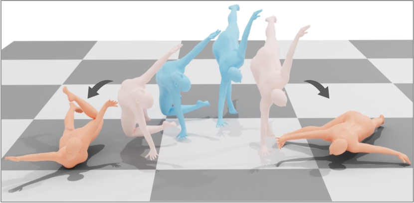
Figure S.5: Stability evaluation using the “Bullet” physics engine. Meshes produced by the baseline method [64] (in orange) topple but IPMAN-O’s meshes (in cyan) remain stable after physics simulation.

C.3 Qualitative Results

Figures S.6 and S.7 show supplemental qualitative results for IPMAN-R and IPMAN-O, respectively.

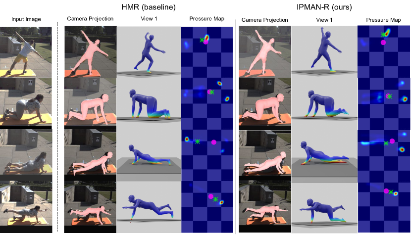
Figure S.6: Additional qualitative evaluation of IPMAN-R on RICH. The first column shows the input images of a subject doing various sports poses. The second and third block of columns show the results of HMR (baseline) and IPMAN-R, respectively. In each block, the first image shows the estimated mesh overlaid on the image. The next three images show different views of the estimated mesh in the world frame. The green sphere illustrates the CoM.

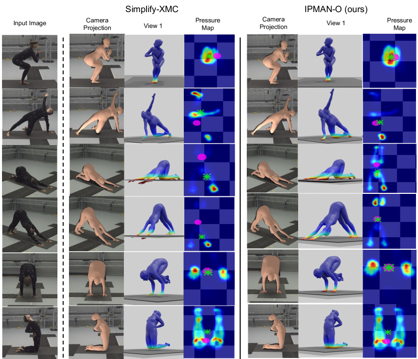
Figure S.7: Qualitative evaluation of IPMAN-O on MoYo. In the first column, the input images of a subject doing yoga poses. The second and third blocks show the results of the SMPLify-XMC and IPMAN-O respectively. In each block, the first and second column show the estimated mesh projected into the image and from a second view. The last images show the pressure map with the CoM (in pink) and the CoP (in green).

Appendix D Stability Evaluation via Physics Simulation

Current physics engines are incompatible with HPS methods, as they approximate SMPL bodies with rigid convex hulls and are non-differentiable. However, using them for posthoc stability evaluation of the estimated meshes is possible. Specifically, we evaluate IPMAN-O and SMPLify-XMC [64] by first, using V-HACD convex decomposition [60] of the estimated body meshes and then by simulating physics as in [29, 84] via the “Bullet” physics engine [10]. We measure the displacement of the human mesh after 100 physics simulation steps; a small displacement denotes a stable pose and vice versa. IPMAN-O produces $14.8\%$ more stable bodies than the baseline [64]; see Fig. S.5.

Appendix E Evaluation of Biomechanical Elements

We use the pressure field defined in Eqn. 2 of the main paper to compute per-point pressure on the SMPL mesh. With this, the pressure heatmap is estimated by summing the per-point pressure projected to the ground-plane. Note that we recover relative pressure as we do not assume availability of ground-truth body mass or anthropometric measurements.

To measure the overlap of the inferred pressure heatmap w.r.t. the ground-truth, we compute the intersection-over-union (IOU) between the two. However, the ZEBRIS pressure sensor captures pressure measurements in the range 10-1200 KPa. Depending upon the contact area and the weight of the subject, some poses may fall outside this range. For instance, a person lying-down only exerts 1-5 kPa of pressure on the ground. To account for this, we tune the sensitivity of our pressure field for every pose and report mean of the best per-sample IOU.

We measure accuracy of our CoP by simply computing the Euclidean distance w.r.t. ground-truth. We call this as CoP error. Again, we report mean of the best CoP error after tuning the sensitivity of our inferred pressure field.

The CoM error is similar to the CoP error, albiet in 3D. It measures the Euclidean distance between the estimated and ground-truth CoM recovered from Vicon Plug-in Gait. Table S.4 presents summary results showing that our inferred pressure, CoP and CoM agrees with the ground-truth.

  Pressure CoM mIOU CoP error (mm) CoM error (mm) IPMAN (Ours) 0.32 57.3 53.3  

Table S.4: Quantitative evaluations of our estimated pressure, CoP and CoM w.r.t. ground-truth in MoYo.

Appendix F IPMAN-O* (Extension of SMPLify-X).

To further explore the effect of our intuitive-physics terms, we extend the optimization method SMPLify-X [68] and name this IPMAN-O* (note that this is different from the main paper’s IPMAN-O that extends SMPLify-XMC). We fit the SMPL-X body model to 2D image keypoints starting from mean pose and shape while exploiting the ground-truth ground plane. Adapted from SMPLify-X [68], we minimize the objective

$$E(\bm{{\beta}},\bm{{\theta}},\bm{{\psi}},\mathbf{t}^{c})= E_{J2D}+E_{\theta}+\lambda_{\beta}E_{\beta}+\lambda_{\psi}E_{\psi}+$$

$$\lambda_{\alpha}E_{\alpha}+\lambda_{\mathcal{C}}E_{\mathcal{C}}+$$ (S.7)

$$\lambda_{s}E_{\text{stability}}+\lambda_{g}E_{\text{ground}}\text{.}$$

The energy term $E_{J2D}$ denotes the 2D re-projection error whereas the remaining terms $E_{\theta}=\lambda_{\theta_{b}}E_{\theta_{b}}+\lambda_{\theta_{f}}E_{\theta_{f}}+\lambda_{\theta_{h}}E_{\theta_{h}}$ represent various priors for body, face, and hand pose. $E_{\beta}$, $E_{\psi}$, $E_{\alpha}$ and $E_{\mathcal{C}}$ are prior terms for body shape, expression, extreme bending and self-penetration (see [68] for details). $E_{S}$ and $E_{G}$ are the stability and ground contact losses. The results in Tab. S.5 show a clear improvement.

Note that SMPLify-X estimates the body’s global orientation $\mathbf{R}^{b}$ and the camera translation $\mathbf{t}^{c}$, while camera rotation $\mathbf{R}^{c}$ and body translation $\mathbf{t}^{b}$ remain zero. In order to apply our IP terms, we use the ground-truth camera rotation $\mathbf{R}^{c}_{w}$ and translation $\mathbf{t}^{c}_{w}$ to transform the estimated mesh from camera to world coordinates. We empirically find that applying the IP terms to the final stage of optimization in SMPLify-X gives more accurate results than applying them to all stages. We hypothesize that this could be due to having a better body initialization before applying the IP terms.

Method	RICH [35]
	MPJPE $\downarrow$	PVE $\downarrow$	BoSE (%) $\uparrow$
SMPLify-X [68]	268.6	228.3	96.9
IPMAN-O* (Ours)	240.9	217.1	98.0

Table S.5: IPMAN-O* compared to the optimization method of [68] on RICH [35].

Appendix G Evaluation on 3DPW

Method	3DPW [88]
	MPJPE $\downarrow$	PMPJPE $\downarrow$
SPIN [49]	97.2	59.6
IPMAN-R (Ours)	96.8	57.1

Table S.6: IPMAN-R compared to the regression method of [49] on 3DPW [88].

3DPW [88] is an outdoor dataset containing pseudo ground-truth SMPL and camera parameters recovered using IMU sensors attached to the actors. As also noted in [102], we find that the ground plane in 3DPW is inconsistent. In fact, two subjects in the same scene can be supported by different ground-planes in the world coordinates. Additionally, 3DPW primarily contains dynamic poses like walking, climbing stairs, parkour, etc. Due to these reasons, 3DPW does not satisfy the core assumptions of IPMAN. Nevertheless, we report results on 3DPW to show that the IP terms do not degrade performance for such datasets; in fact, we see a slight improvement in performance as illustrated in Table S.6. This makes IPMAN applicable to everyday motion without needing special care.

References

- [1] Ijaz Akhter and Michael J. Black. Pose-conditioned joint angle limits for 3D human pose reconstruction. In Computer Vision and Pattern Recognition (CVPR), pages 1446–1455, 2015.
- [2] Rıza Alp Güler, Natalia Neverova, and Iasonas Kokkinos. DensePose: Dense human pose estimation in the wild. In Computer Vision and Pattern Recognition (CVPR), pages 7297–7306, 2018.
- [3] Erling D. Andersen and Knud D. Andersen. The Mosek interior point optimizer for linear programming: An implementation of the homogeneous algorithm. In High Performance Optimization, 2000.
- [4] Mykhaylo Andriluka, Leonid Pishchulin, Peter Gehler, and Bernt Schiele. 2D human pose estimation: New benchmark and state of the art analysis. In Computer Vision and Pattern Recognition (CVPR), pages 3686–3693, 2014.
- [5] Dragomir Anguelov, Praveen Srinivasan, Daphne Koller, Sebastian Thrun, Jim Rodgers, and James Davis. SCAPE: Shape completion and animation of people. Transactions on Graphics (TOG), 24:408–416, 2005.
- [6] Michael Barnett-Cowan, Roland W. Fleming, Manish Singh, and Heinrich H. Bülthoff. Perceived object stability depends on multisensory estimates of gravity. PLOS ONE, 6(4):1–5, 2011.
- [7] Federica Bogo, Angjoo Kanazawa, Christoph Lassner, Peter Gehler, Javier Romero, and Michael J. Black. Keep it SMPL: Automatic estimation of 3D human pose and shape from a single image. In European Conference on Computer Vision (ECCV), volume 9909, pages 561–578, 2016.
- [8] Marcus A. Brubaker, David J. Fleet, and Aaron Hertzmann. Physics-based person tracking using the anthropomorphic walker. International Journal of Computer Vision (IJCV), 87(1–2):140–155, 2010.
- [9] Marcus A. Brubaker, Leonid Sigal, and David J. Fleet. Estimating contact dynamics. In Computer Vision and Pattern Recognition (CVPR), pages 2389–2396, 2009.
- [10] Bullet real-time physics simulation. https://pybullet.org.
- [11] Zhe Cao, Gines Hidalgo, Tomas Simon, Shih-En Wei, and Yaser Sheikh. OpenPose: Realtime multi-person 2D pose estimation using part affinity fields. Transactions on Pattern Analysis and Machine Intelligence (TPAMI), 43(1):172–186, 2021.
- [12] Yixin Chen, Sai Kumar Dwivedi, Michael J. Black, and Dimitrios Tzionas. Detecting human-object contact in images. In Computer Vision and Pattern Recognition (CVPR), June 2023.
- [13] Vasileios Choutas, Georgios Pavlakos, Timo Bolkart, Dimitrios Tzionas, and Michael J. Black. Monocular expressive body regression through body-driven attention. In European Conference on Computer Vision (ECCV), volume 12355, pages 20–40, 2020.
- [14] Henry M. Clever, Zackory M. Erickson, Ariel Kapusta, Greg Turk, C. Karen Liu, and Charles C. Kemp. Bodies at rest: 3D human pose and shape estimation from a pressure image using synthetic data. In Computer Vision and Pattern Recognition (CVPR), pages 6214–6223, 2020.
- [15] Enric Corona, Albert Pumarola, Guillem Alenyà, Gerard Pons-Moll, and Francesc Moreno-Noguer. SMPLicit: Topology-aware generative model for clothed people. In Computer Vision and Pattern Recognition (CVPR), pages 11875–11885, 2021.
- [16] Taosha Fan, Kalyan Vasudev Alwala, Donglai Xiang, Weipeng Xu, Todd Murphey, and Mustafa Mukadam. Revitalizing optimization for 3D human pose and shape estimation: A sparse constrained formulation. In International Conference on Computer Vision (ICCV), pages 11437–11446, 2021.
- [17] Zicong Fan, Omid Taheri, Dimitrios Tzionas, Muhammed Kocabas, Manuel Kaufmann, Michael J. Black, and Otmar Hilliges. ARCTIC: A dataset for dexterous bimanual hand-object manipulation. In Computer Vision and Pattern Recognition (CVPR), June 2023.
- [18] Yao Feng, Vasileios Choutas, Timo Bolkart, Dimitrios Tzionas, and Michael J. Black. Collaborative regression of expressive bodies using moderation. In International Conference on 3D Vision (3DV), pages 792–804, 2021.
- [19] Mihai Fieraru, Mihai Zanfir, Teodor Alexandru Szente, Eduard Gabriel Bazavan, Vlad Olaru, and Cristian Sminchisescu. REMIPS: Physically consistent 3D reconstruction of multiple interacting people under weak supervision. In Conference on Neural Information Processing Systems (NeurIPS), volume 34, 2021.
- [20] Mihai Fieraru, Mihai Zanfir, Silviu-Cristian Pirlea, Vlad Olaru, and Cristian Sminchisescu. AIFit: Automatic 3D human-interpretable feedback models for fitness training. In Computer Vision and Pattern Recognition (CVPR), pages 9919–9928, 2021.
- [21] Erik Gärtner, Mykhaylo Andriluka, Erwin Coumans, and Cristian Sminchisescu. Differentiable dynamics for articulated 3D human motion reconstruction. In Computer Vision and Pattern Recognition (CVPR), pages 13180–13190, 2022.
- [22] Erik Gärtner, Mykhaylo Andriluka, Hongyi Xu, and Cristian Sminchisescu. Trajectory optimization for physics-based reconstruction of 3D human pose from monocular video. In Computer Vision and Pattern Recognition (CVPR), pages 13096–13105, 2022.
- [23] Ke Gong, Yiming Gao, Xiaodan Liang, Xiaohui Shen, Meng Wang, and Liang Lin. Graphonomy: Universal human parsing via graph transfer learning. In Computer Vision and Pattern Recognition (CVPR), pages 7450–7459, 2019.
- [24] Shanyan Guan, Jingwei Xu, Yunbo Wang, Bingbing Ni, and Xiaokang Yang. Bilevel online adaptation for out-of-domain human mesh reconstruction. In Computer Vision and Pattern Recognition (CVPR), pages 10472–10481, 2021.
- [25] Riza Alp Güler and Iasonas Kokkinos. HoloPose: Holistic 3D human reconstruction in-the-wild. In Computer Vision and Pattern Recognition (CVPR), pages 10876–10886, 2019.
- [26] Shreyas Hampali, Mahdi Rad, Markus Oberweger, and Vincent Lepetit. HOnnotate: A method for 3D annotation of hand and object poses. In Computer Vision and Pattern Recognition (CVPR), pages 3193–3203, 2020.
- [27] Mohamed Hassan, Vasileios Choutas, Dimitrios Tzionas, and Michael J. Black. Resolving 3D human pose ambiguities with 3D scene constraints. In International Conference on Computer Vision (ICCV), pages 2282–2292, 2019.
- [28] Mohamed Hassan, Partha Ghosh, Joachim Tesch, Dimitrios Tzionas, and Michael J. Black. Populating 3D scenes by learning human-scene interaction. In Computer Vision and Pattern Recognition (CVPR), pages 14708–14718, 2021.
- [29] Yana Hasson, Gül Varol, Dimitrios Tzionas, Igor Kalevatykh, Michael J. Black, Ivan Laptev, and Cordelia Schmid. Learning joint reconstruction of hands and manipulated objects. In Computer Vision and Pattern Recognition (CVPR), pages 11807–11816, 2019.
- [30] Havok: Customizable, fully multithreaded, and highly optimized physics simulation. http://www.havok.com.
- [31] Eric Heiden, David Millard, Erwin Coumans, Yizhou Sheng, and Gaurav S. Sukhatme. NeuralSim: Augmenting differentiable simulators with neural networks. In International Conference on Robotics and Automation (ICRA), pages 9474–9481, 2021.
- [32] At L. Hof. The equations of motion for a standing human reveal three mechanisms for balance. Journal of Biomechanics, 40(2):451–457, 2007.
- [33] At L. Hof. The “extrapolated center of mass” concept suggests a simple control of balance in walking. Human movement science, 27(1):112–125, 2008.
- [34] At L. Hof, M. G. J. Gazendam, and Sinke W. E. The condition for dynamic stability. Journal of Biomechanics, 38(1):1–8, 2005.
- [35] Chun-Hao Huang, Hongwei Yi, Markus Höschle, Matvey Safroshkin, Tsvetelina Alexiadis, Senya Polikovsky, Daniel Scharstein, and Michael Black. Capturing and inferring dense full-body human-scene contact. In Computer Vision and Pattern Recognition (CVPR), pages 13264–13275, 2022.
- [36] Leslie Ikemoto, Okan Arikan, and David Forsyth. Knowing when to put your foot down. In Symposium on Interactive 3D Graphics (SI3D), page 49–53, 2006.
- [37] Catalin Ionescu, Dragos Papava, Vlad Olaru, and Cristian Sminchisescu. Human3.6M: Large scale datasets and predictive methods for 3D human sensing in natural environments. Transactions on Pattern Analysis and Machine Intelligence (TPAMI), 36(7):1325–1339, 2014.
- [38] Wen Jiang, Nikos Kolotouros, Georgios Pavlakos, Xiaowei Zhou, and Kostas Daniilidis. Coherent reconstruction of multiple humans from a single image. In Computer Vision and Pattern Recognition (CVPR), pages 5578–5587, 2020.
- [39] Sam Johnson and Mark Everingham. Clustered pose and nonlinear appearance models for human pose estimation. In British Machine Vision Conference (BMVC), pages 1–11, 2010.
- [40] Sam Johnson and Mark Everingham. Learning effective human pose estimation from inaccurate annotation. In Computer Vision and Pattern Recognition (CVPR), pages 1465–1472, 2011.
- [41] Hanbyul Joo, Natalia Neverova, and Andrea Vedaldi. Exemplar fine-tuning for 3D human pose fitting towards in-the-wild 3D human pose estimation. In International Conference on 3D Vision (3DV), pages 42–52, 2021.
- [42] Hanbyul Joo, Tomas Simon, and Yaser Sheikh. Total capture: A 3D deformation model for tracking faces, hands, and bodies. In Computer Vision and Pattern Recognition (CVPR), pages 8320–8329, 2018.
- [43] Angjoo Kanazawa, Michael J. Black, David W. Jacobs, and Jitendra Malik. End-to-end recovery of human shape and pose. In Computer Vision and Pattern Recognition (CVPR), pages 7122–7131, 2018.
- [44] Angjoo Kanazawa, Jason Y. Zhang, Panna Felsen, and Jitendra Malik. Learning 3D human dynamics from video. Computer Vision and Pattern Recognition (CVPR), pages 5607–5616, 2019.
- [45] Rawal Khirodkar, Shashank Tripathi, and Kris Kitani. Occluded human mesh recovery. In Computer Vision and Pattern Recognition (CVPR), pages 1705–1715, 2022.
- [46] Muhammed Kocabas, Nikos Athanasiou, and Michael J. Black. VIBE: Video inference for human body pose and shape estimation. In Computer Vision and Pattern Recognition (CVPR), pages 5252–5262, 2020.
- [47] Muhammed Kocabas, Chun-Hao P. Huang, Otmar Hilliges, and Michael J. Black. PARE: Part attention regressor for 3D human body estimation. In International Conference on Computer Vision (ICCV), pages 11127–11137, 2021.
- [48] Muhammed Kocabas, Chun-Hao P. Huang, Joachim Tesch, Lea Müller, Otmar Hilliges, and Michael J. Black. SPEC: Seeing people in the wild with an estimated camera. In International Conference on Computer Vision (ICCV), pages 11035–11045, 2021.
- [49] Nikos Kolotouros, Georgios Pavlakos, Michael J. Black, and Kostas Daniilidis. Learning to reconstruct 3D human pose and shape via model-fitting in the loop. In International Conference on Computer Vision (ICCV), pages 2252–2261, 2019.
- [50] Nikos Kolotouros, Georgios Pavlakos, and Kostas Daniilidis. Convolutional mesh regression for single-image human shape reconstruction. In Computer Vision and Pattern Recognition (CVPR), pages 4496–4505, 2019.
- [51] Jiefeng Li, Siyuan Bian, Chao Xu, Gang Liu, Gang Yu, and Cewu Lu. D&D: Learning human dynamics from dynamic camera. In European Conference on Computer Vision (ECCV), 2022.
- [52] Jiefeng Li, Chao Xu, Zhicun Chen, Siyuan Bian, Lixin Yang, and Cewu Lu. HybrIK: A hybrid analytical-neural inverse kinematics solution for 3D human pose and shape estimation. In Computer Vision and Pattern Recognition (CVPR), pages 3383–3393, 2021.
- [53] Zhihao Li, Jianzhuang Liu, Zhensong Zhang, Songcen Xu, and Youliang Yan. CLIFF: Carrying location information in full frames into human pose and shape estimation. In ECCV, volume 13665, pages 590–606, 2022.
- [54] Kevin Lin, Lijuan Wang, and Zicheng Liu. End-to-end human pose and mesh reconstruction with transformers. In Computer Vision and Pattern Recognition (CVPR), pages 1954–1963, 2021.
- [55] Tsung-Yi Lin, Michael Maire, Serge J. Belongie, James Hays, Pietro Perona, Deva Ramanan, Piotr Dollár, and C. Lawrence Zitnick. Microsoft COCO: Common objects in context. In European Conference on Computer Vision (ECCV), volume 8693, pages 740–755, 2014.
- [56] Matthew Loper, Naureen Mahmood, Javier Romero, Gerard Pons-Moll, and Michael J. Black. SMPL: A skinned multi-person linear model. Transactions on Graphics (TOG), 34(6):248:1–248:16, 2015.
- [57] Camillo Lugaresi, Jiuqiang Tang, Hadon Nash, Chris McClanahan, Esha Uboweja, Michael Hays, Fan Zhang, Chuo-Ling Chang, Ming Guang Yong, Juhyun Lee, Wan-Teh Chang, Wei Hua, Manfred Georg, and Matthias Grundmann. MediaPipe: A framework for building perception pipelines. In Computer Vision and Pattern Recognition Workshops (CVPRw), 2019.
- [58] Yiyue Luo, Yunzhu Li, Michael Foshey, Wan Shou, Pratyusha Sharma, Tomás Palacios, Antonio Torralba, and Wojciech Matusik. Intelligent carpet: Inferring 3D human pose from tactile signals. In Computer Vision and Pattern Recognition (CVPR), pages 11255–11265, 2021.
- [59] Naureen Mahmood, Nima Ghorbani, Nikolaus F. Troje, Gerard Pons-Moll, and Michael J. Black. AMASS: Archive of motion capture as surface shapes. In International Conference on Computer Vision (ICCV), pages 5441–5450, 2019.
- [60] Khaled Mamou, E Lengyel, and A Peters. Volumetric hierarchical approximate convex decomposition. In Game Engine Gems 3, pages 141–158. AK Peters, 2016.
- [61] Dushyant Mehta, Helge Rhodin, Dan Casas, Pascal V. Fua, Oleksandr Sotnychenko, Weipeng Xu, and Christian Theobalt. Monocular 3D human pose estimation in the wild using improved CNN supervision. International Conference on 3D Vision (3DV), pages 506–516, 2017.
- [62] Dushyant Mehta, Srinath Sridhar, Oleksandr Sotnychenko, Helge Rhodin, Mohammad Shafiei, Hans-Peter Seidel, Weipeng Xu, Dan Casas, and Christian Theobalt. VNect: Real-time 3D human pose estimation with a single RGB camera. Transactions on Graphics (TOG), 36(4):44:1–44:14, 2017.
- [63] Gyeongsik Moon and Kyoung Mu Lee. I2L-MeshNet: Image-to-lixel prediction network for accurate 3D human pose and mesh estimation from a single RGB image. In European Conference on Computer Vision (ECCV), volume 12352, pages 752–768, 2020.
- [64] Lea Müller, Ahmed A. A. Osman, Siyu Tang, Chun-Hao P. Huang, and Michael J. Black. On self-contact and human pose. In Computer Vision and Pattern Recognition (CVPR), pages 9990–9999, 2021.
- [65] NVIDIA PhysX: A scalable multi-platform physics simulation solution. https://developer.nvidia.com/physx-sdk.
- [66] Yi-Chung Pai. Movement termination and stability in standing. Exercise and sport sciences reviews, 31(1):19–25, 2003.
- [67] Priyanka Patel, Chun-Hao P Huang, Joachim Tesch, David T Hoffmann, Shashank Tripathi, and Michael J Black. AGORA: Avatars in geography optimized for regression analysis. In Computer Vision and Pattern Recognition (CVPR), pages 13468–13478, 2021.
- [68] Georgios Pavlakos, Vasileios Choutas, Nima Ghorbani, Timo Bolkart, Ahmed A. A. Osman, Dimitrios Tzionas, and Michael J. Black. Expressive body capture: 3D hands, face, and body from a single image. In Computer Vision and Pattern Recognition (CVPR), pages 10975–10985, 2019.
- [69] Xue Bin Peng, Pieter Abbeel, Sergey Levine, and Michiel van de Panne. DeepMimic: Example-guided deep reinforcement learning of physics-based character skills. Transactions on Graphics (TOG), 37(4):1–14, 2018.
- [70] Davis Rempe, Tolga Birdal, Aaron Hertzmann, Jimei Yang, Srinath Sridhar, and Leonidas J. Guibas. HuMoR: 3D human motion model for robust pose estimation. In International Conference on Computer Vision (ICCV), pages 11468–11479, 2021.
- [71] Davis Rempe, Leonidas J. Guibas, Aaron Hertzmann, Bryan Russell, Ruben Villegas, and Jimei Yang. Contact and human dynamics from monocular video. In European Conference on Computer Vision (ECCV), volume 12350, pages 71–87, 2020.
- [72] Ralph Tyrell Rockafellar. Convex analysis. Princeton university press, 2015.
- [73] Grégory Rogez, James Steven Supancic, and Deva Ramanan. Understanding everyday hands in action from RGB-D images. In International Conference on Computer Vision (ICCV), pages 3889–3897, 2015.
- [74] Yu Rong, Takaaki Shiratori, and Hanbyul Joo. FrankMocap: A monocular 3D whole-body pose estimation system via regression and integration. In International Conference on Computer Vision Workshops (ICCVw), pages 1749–1759, 2021.
- [75] Nadine Rueegg, Shashank Tripathi, Konrad Schindler, Michael J. Black, and Silvia Zuffi. BITE: Beyond priors for improved three-D dog pose estimation. In Computer Vision and Pattern Recognition (CVPR), June 2023.
- [76] Jesse Scott, Bharadwaj Ravichandran, Christopher Funk, Robert T Collins, and Yanxi Liu. From image to stability: Learning dynamics from human pose. In European Conference on Computer Vision (ECCV), volume 12368, pages 536–554, 2020.
- [77] Mingyi Shi, Kfir Aberman, Andreas Aristidou, Taku Komura, Dani Lischinski, Daniel Cohen-Or, and Baoquan Chen. MotioNet: 3D human motion reconstruction from monocular video with skeleton consistency. Transactions on Graphics (TOG), 40(1):1:1–1:15, 2021.
- [78] Soshi Shimada, Vladislav Golyanik, Weipeng Xu, Patrick Pérez, and Christian Theobalt. Neural monocular 3D human motion capture with physical awareness. Transactions on Graphics (TOG), 40(4), 2021.
- [79] Soshi Shimada, Vladislav Golyanik, Weipeng Xu, and Christian Theobalt. PhysCap: Physically plausible monocular 3D motion capture in real time. Transactions on Graphics (TOG), 39(6):235:1–235:16, 2020.
- [80] Yu Sun, Qian Bao, Wu Liu, Yili Fu, Michael J. Black, and Tao Mei. Monocular, one-stage, regression of multiple 3D people. In International Conference on Computer Vision (ICCV), pages 11179–11188, 2021.
- [81] Yu Sun, Yun Ye, Wu Liu, Wenpeng Gao, Yili Fu, and Tao Mei. Human mesh recovery from monocular images via a skeleton-disentangled representation. In International Conference on Computer Vision (ICCV), pages 5348–5357, 2019.
- [82] Yating Tian, Hongwen Zhang, Yebin Liu, and limin Wang. Recovering 3D human mesh from monocular images: A survey. arXiv:2203.01923, 2022.
- [83] Shashank Tripathi, Siddhant Ranade, Ambrish Tyagi, and Amit K. Agrawal. PoseNet3D: Learning temporally consistent 3D human pose via knowledge distillation. In International Conference on 3D Vision (3DV), pages 311–321, 2020.
- [84] Dimitrios Tzionas, Luca Ballan, Abhilash Srikantha, Pablo Aponte, Marc Pollefeys, and Juergen Gall. Capturing hands in action using discriminative salient points and physics simulation. International Journal of Computer Vision (IJCV), 118:172–193, 2016.
- [85] Laurens van der Maaten and Geoffrey Hinton. Visualizing data using t-sne. Journal of Machine Learning Research (JMLR), 9(86):2579–2605, 2008.
- [86] Manisha Verma, Sudhakar Kumawat, Yuta Nakashima, and Shanmuganathan Raman. Yoga-82: A new dataset for fine-grained classification of human poses. In Computer Vision and Pattern Recognition Workshops (CVPRw), pages 1038–1039, 2020.
- [87] Ruben Villegas, Duygu Ceylan, Aaron Hertzmann, Jimei Yang, and Jun Saito. Contact-aware retargeting of skinned motion. In International Conference on Computer Vision (ICCV), pages 9720–9729, 2021.
- [88] Timo von Marcard, Roberto Henschel, Michael J. Black, Bodo Rosenhahn, and Gerard Pons-Moll. Recovering accurate 3D human pose in the wild using IMUs and a moving camera. In European Conference on Computer Vision (ECCV), volume 11214, pages 614–631, 2018.
- [89] Marek Vondrak, Leonid Sigal, and Odest Chadwicke Jenkins. Physical simulation for probabilistic motion tracking. In Computer Vision and Pattern Recognition (CVPR), pages 1–8, 2008.
- [90] Eric W. Weisstein. Triangle point picking. https://mathworld.wolfram.com/TrianglePointPicking.html, 2014. From MathWorld – A Wolfram Web Resource.
- [91] Zhenzhen Weng and Serena Yeung. Holistic 3D human and scene mesh estimation from single view images. In Computer Vision and Pattern Recognition (CVPR), pages 334–343, 2020.
- [92] David A. Winter. A.B.C. (Anatomy, Biomechanics and Control) of balance during standing and walking. Waterloo Biomechanics, 1995.
- [93] David A. Winter. Human balance and posture control during standing and walking. Gait & Posture, 3(4):193–214, 1995.
- [94] Donglai Xiang, Hanbyul Joo, and Yaser Sheikh. Monocular total capture: Posing face, body, and hands in the wild. In Computer Vision and Pattern Recognition (CVPR), pages 10957–10966, 2019.
- [95] Donglai Xiang, Fabian Prada, Chenglei Wu, and Jessica Hodgins. MonoClothCap: Towards temporally coherent clothing capture from monocular RGB video. In International Conference on 3D Vision (3DV), pages 322–332, 2020.
- [96] Kevin Xie, Tingwu Wang, Umar Iqbal, Yunrong Guo, Sanja Fidler, and Florian Shkurti. Physics-based human motion estimation and synthesis from videos. In International Conference on Computer Vision (ICCV), pages 11532–11541, 2021.
- [97] Xianghui Xie, Bharat Lal Bhatnagar, and Gerard Pons-Moll. CHORE: Contact, human and object reconstruction from a single RGB image. In European Conference on Computer Vision (ECCV), 2022.
- [98] Yuliang Xiu, Jinlong Yang, Xu Cao, Dimitrios Tzionas, and Michael J. Black. ECON: Explicit clothed humans optimized via normal integration. In Computer Vision and Pattern Recognition (CVPR), 2023.
- [99] Hongyi Xu, Eduard Gabriel Bazavan, Andrei Zanfir, William T. Freeman, Rahul Sukthankar, and Cristian Sminchisescu. GHUM & GHUML: Generative 3D human shape and articulated pose models. In Computer Vision and Pattern Recognition (CVPR), pages 6183–6192, 2020.
- [100] Masanobu Yamamoto and Katsutoshi Yagishita. Scene constraints-aided tracking of human body. In Computer Vision and Pattern Recognition (CVPR), pages 151–156, 2000.
- [101] Hongwei Yi, Chun-Hao P. Huang, Shashank Tripathi, Lea Hering, Justus Thies, and Michael J. Black. MIME: Human-aware 3D scene generation. In Computer Vision and Pattern Recognition (CVPR), June 2023.
- [102] Ye Yuan, Umar Iqbal, Pavlo Molchanov, Kris Kitani, and Jan Kautz. GLAMR: Global occlusion-aware human mesh recovery with dynamic cameras. In Computer Vision and Pattern Recognition (CVPR), pages 11028–11039, 2022.
- [103] Ye Yuan and Kris Kitani. 3D ego-pose estimation via imitation learning. In European Conference on Computer Vision (ECCV), volume 11220, pages 735–750, 2018.
- [104] Ye Yuan, Shih-En Wei, Tomas Simon, Kris Kitani, and Jason Saragih. SimPoE: Simulated character control for 3D human pose estimation. In Computer Vision and Pattern Recognition (CVPR), pages 7159–7169, 2021.
- [105] Andrei Zanfir, Eduard Gabriel Bazavan, Hongyi Xu, William T Freeman, Rahul Sukthankar, and Cristian Sminchisescu. Weakly supervised 3D human pose and shape reconstruction with normalizing flows. In European Conference on Computer Vision (ECCV), pages 465–481, 2020.
- [106] Andrei Zanfir, Elisabeta Marinoiu, and Cristian Sminchisescu. Monocular 3D pose and shape estimation of multiple people in natural scenes – the importance of multiple scene constraints. In Computer Vision and Pattern Recognition (CVPR), pages 2148–2157, 2018.
- [107] Ailing Zeng, Lei Yang, Xuan Ju, Jiefeng Li, Jianyi Wang, and Qiang Xu. SmoothNet: A plug-and-play network for refining human poses in videos. In European Conference on Computer Vision (ECCV), volume 13665, pages 625–642, 2022.
- [108] Wang Zeng, Wanli Ouyang, Ping Luo, Wentao Liu, and Xiaogang Wang. 3D human mesh regression with dense correspondence. In Computer Vision and Pattern Recognition (CVPR), 2020.
- [109] Cha Zhang and Tsuhan Chen. Efficient feature extraction for 2d/3d objects in mesh representation. In Proceedings 2001 International Conference on Image Processing (Cat. No. 01CH37205), volume 3, pages 935–938. IEEE, 2001.
- [110] Hongwen Zhang, Yating Tian, Xinchi Zhou, Wanli Ouyang, Yebin Liu, Limin Wang, and Zhenan Sun. PyMAF: 3D human pose and shape regression with pyramidal mesh alignment feedback loop. In International Conference on Computer Vision (ICCV), pages 11426–11436, 2021.
- [111] Jianfeng Zhang, Dongdong Yu, Jun Hao Liew, Xuecheng Nie, and Jiashi Feng. Body meshes as points. In Computer Vision and Pattern Recognition (CVPR), pages 546–556, 2021.
- [112] Jason Y. Zhang, Sam Pepose, Hanbyul Joo, Deva Ramanan, Jitendra Malik, and Angjoo Kanazawa. Perceiving 3D human-object spatial arrangements from a single image in the wild. In European Conference on Computer Vision (ECCV), volume 12357, pages 34–51, 2020.
- [113] Siwei Zhang, Yan Zhang, Federica Bogo, Marc Pollefeys, and Siyu Tang. Learning motion priors for 4D human body capture in 3D scenes. In International Conference on Computer Vision (ICCV), pages 11343–11353, 2021.
- [114] Tianshu Zhang, Buzhen Huang, and Yangang Wang. Object-occluded human shape and pose estimation from a single color image. In Computer Vision and Pattern Recognition (CVPR), pages 7374–7383, 2020.
- [115] Ce Zheng, Wenhan Wu, Chen Chen, Taojiannan Yang, Sijie Zhu, Ju Shen, Nasser Kehtarnavaz, and Mubarak Shah. Deep learning-based human pose estimation: A survey. arXiv:2012.13392, 2022.
- [116] Yi Zhou, Connelly Barnes, Jingwan Lu, Jimei Yang, and Hao Li. On the continuity of rotation representations in neural networks. In Computer Vision and Pattern Recognition (CVPR), pages 5745–5753, 2019.
- [117] Yuxiao Zhou, Marc Habermann, Ikhsanul Habibie, Ayush Tewari, Christian Theobalt, and Feng Xu. Monocular real-time full body capture with inter-part correlations. In Computer Vision and Pattern Recognition (CVPR), pages 4811–4822, 2021.
- [118] Yuliang Zou, Jimei Yang, Duygu Ceylan, Jianming Zhang, Federico Perazzi, and Jia-Bin Huang. Reducing footskate in human motion reconstruction with ground contact constraints. In Winter Conference on Applications of Computer Vision (WACV), pages 459–468, 2020.