Kondo $s$-$d$ exchange interaction in the CuO₂ plane as the long sought mechanism of high temperature superconductivity in cuprates

Abstract

The well-known Pavarini et al. [Phys. Rev. Lett. 87, 047003 (2001)] correlation between the critical temperature $T_{c,\,\mathrm{max}}$ and the shape of the Fermi contour of the optimally hole-doped cuprates are explained within the framework of the BCS theory with Kondo exchange interaction incorporated as a pairing mechanism. The strong influence of the relative position of the Cu4$s$ level with respect to the Cu3$d_{x^{2}-y^{2}}$ level on the critical temperature $T_{c}$ reveals why the s-d hybridization of the conduction band is so important. This hybridization is proportional to the s-d exchange scattering amplitude between the conduction electrons – the mechanism of $d$-wave pairing in the CuO₂ plane. In other words the Kondo interaction considered as a pairing mechanism in the CuO₂ plane gives a natural explanation of the correlation between the critical temperature and the shape of the Fermi contour. The lack of an alternative explanation for the description of the critical temperature of optimally doped cuprates for several decades gives a hint that the long sought pairing mechanism has already been found.

I Introduction. What determines $T_{c,\,\mathrm{max}}$?

Condensed matter is without a doubt one of the most sophisticated fields of physics, if not in science. One of its most important and still open problem is the mechanism of High-$T_{c}$ Superconductivity (HTC) discovered by Bednorz and Müller [1] more than 30 years ago. On the problem of models and mechanisms of High-Temperature Superconductivity (HTS) several conferences were held [2] and a review of the suggested ideas can be easily performed: all processes in the condensed matter was considered as the possible mechanism of HTS. In the heroic initial period of HTS physics, up to 1/8 of submitted manuscripts to Phys. Rev. Lett. were devoted on HTS problem [3, 4]. Step by step for a period of 36 years 100-200 thousand experimental papers studying HTS were published. A natural problems arises: which of those experiments can be considered as a crucial for our understanding of the mechanism of HTS? What does the critical temperature $T_{c}$ depend on and with what does it correlate? The answers to these questions seem not to be much closer as they were after the time of the discovery of HTS. First mechanism proposals [5, 6] lead to numerous models [3, 7, 4, 8, 9, 10, 11, 12] but no clear winner is in sight yet. Now it seems strange that the crucial experiment is a numerical one; a method which has never lead to Nobel prize in physics. The high-$T_{c}$ cuprates have attracted attention just because the critical temperature can be high. But for every compound the critical temperature $T_{c}$ depend on doping or the chemical potential. Let us recall the well-known parabolic approximation [13]

$$T_{c}/T_{c,\,\mathrm{max}}=1-82.6\,(\tilde{p}-0.16)^{2}.$$ (1)

close to optimal doping of $\tilde{p}_{\mathrm{opt}}=0.16$ holes per Cu ion in CuO₂ plane. This maximum is far from metal-insulator transition and close to this maximum high-$T_{c}$ cuprates are in first approximation normal metal. Normal metals for which electron band theory is well applicable. And ab initio calculated Fermi surface is in excellent agreement with Angle Resolved Photo Emission Spectroscopy (ARPES) data. Moreover, even BCS spectrum of the normal excited states is observable in some cases. Additionally close to the optimal doping the pseudo gap, if any, is small and has weak influence on $T_{c}$ and thermodynamic properties of cuprates. These circumstances allow us to use traditional approach of electron band calculations and BCS pairing at least for initial analysis what determines the critical temperature $T_{c,\,\mathrm{max}}$ at optimal doping. Some preliminary qualitative analysis was performed long time ago [14]; here we give detailed analysis. Technical details of the Linear Combination of Atomic Orbitals (LCAO) approximation of the electron band structure of CuO₂ plane and matrix elements of the Kondo interaction in this approximation are given in the textbook [15] here we concentrate in the next section on the results giving the possibility to analyze what determines $T_{c,\,\mathrm{max}}$.

II Results

All HTS cuprates contain CuO₂ plane, but why is the critical temperature $T_{c,\,\mathrm{max}}$ so different even for optimally doped superconductors with $\tilde{p}=0.16$ holes per Cu ion [13]? A hint of the nature of high temperature superconductivity in cuprates in the LCAO calculations by Andersen et al. [16, 17] was noticed by Röhler [18, 19] who suggested that the hybridization between the Cu$3d$ and Cu$4s$ is a crucial parameter for the CuO₂ plane. This hint was strongly confirmed by the remarkable correlation between the Cu$4s$ energy level and the critical temperature $T_{c,\,\mathrm{max}}$ from band calculations by Pavarini et al. [20]. It turns out that $T_{c,\,\mathrm{max}}$ for optimally doped cuprates strongly correlates with dimensionless parameter $t^{\prime}/t$ determining the shape of the Fermi contour interpolated by the formula

$$-2t\,[\cos p_{x}+\cos p_{y}]+4t^{\prime}\cos p_{x}\cos p_{y}=\mathrm{const},$$ (2)

$$\;\,p_{x}\equiv a_{0}P_{x}/\hbar,\quad p_{y}\equiv a_{0}P_{y}/\hbar,\quad(p_{x},\,p_{y})\in(0,\,2\pi),$$

where $a_{0}$ is the Cu-Cu distance (the lattice constant), and $\mathbf{P}$ is the electron quasi-momentum moving in the CuO₂ plane.

The correlation $T_{c,\,\mathrm{max}}$ versus $t^{\prime}/t$ by Pavarini et al. [20] has obtained broad recognition and is cited more than 555 times even now, unfortunately as a curious empirical correlation without microscopic theoretical understanding. In Fig. 1 we reproduce this correlation, as we add to the electron band calculations new data for $t^{\prime}/t$ obtained by ARPES experiments, as ARPES is widely used for studying of cuprates [21, 22, 23, 24].

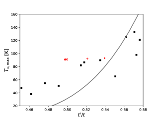
Figure 1: Pavarini et al. [20] (_■) correlation between the critical temperature for optimally doped cuprates $T_{c,\,\mathrm{max}}$ and dimensionless $t^{\prime}/t$ parameter. The $t^{\prime}/t$ parameter itself is exactly a linear function of the BCS coupling parameter $\lambda$ supposing constant $J_{sd}=5.593$ eV. According to our traditional BCS interpretation (solid line) this band-structure trend describes $T_{c,\,\mathrm{max}}$-$\lambda$ correlation for the s-d exchange amplitude $J_{sd}$ approximately equal for all cuprates. Here ARPES data is included with ($\mathbf{\star}$) by Zonno et al. [25, Fig. 5c] and ( $\mathbf{\times}$) by Zhang et al. [26, Fig. 1] for optimally doped Bi-2212, and ( $\mathbf{+}$) by Nakayama et al. [27, Fig. 1] and ( $\mathbf{\bullet}$) by Okawa et al. [28, Fig. 1] for optimally doped YBCO.

The continuous line in this figure is a guiding for the eye theoretical curve. The grouping of the experimental points near to a universal curve points out that nature wishes to tell us something and the purpose of the present article is to reveal God’s plan. Here we feel obliged to present a short apology of the electron band theory. No doubts for underdoped cuprates the Fermi contour is not well defined, but Pavarini et al. [20] correlations refer for optimally doped cuprates for which the electron band theory is well applicable. It is not necessary to cite hundreds paper on electron band calculation for layered cuprates the perfect agreement between electron band calculations and experimentally observed by ARPES Fermi contours is convincing for every skeptical adept of the strong correlations.

According to the original consideration by Mott every metal becomes insulator if we gradually increase the lattice constant, but it is not an argument that in every work on physics of metals metal insulator transition needs to be derived or even considered. In short, optimally doped cuprates are in first approximations normal metals for which ab intio calculated dispersion of the conduction band is in acceptable agreement with the experimentally observed one. Concerning the statistical properties for optimally doped superconductors, BCS-Bogoliubov spectrum of the electron excitations has also been experimentally confirmed [29]. That is why the BCS trial function approach gives acceptable evaluation of the thermodynamic and kinetic properties of optimally doped cuprates. For them the pseudogap is too small if any to perturb and destroy the BCS picture. Concerning normal state properties as strong anisotropy of the normal state scattering rate and the linear temperature dependence of the in plane resistivity, they also have conventional explanation in the framework of the normal metal theory; see for example Refs. [30, 31] and references therein.

Often the choice of the variables is important for the future analysis and in Fig. 2 the same data is represented by logarithm of the ordinate and the reciprocal value of the abscissa, i.e in Fig. 2 the same correlation between the shape and content in the plot (-$\ln T_{c}$ versus $t/t^{\prime}$) is depicted.

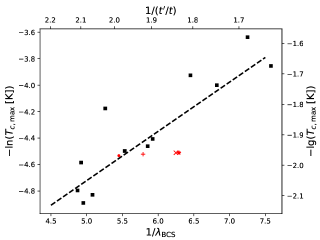
Figure 2: BCS correlation between the critical temperature $-\ln(T_{c,\,\mathrm{max}})$, $t^{\prime}/t$ parameter and BCS coupling constant $\lambda$. According to Eq. (14) this should be in initial approximation a straight line. The high correlation coefficient $\rho\approx 0.85$ is a hint that nature wishes to tell us something. The straight line is derived supposing that for different cuprates only the position of the 4$s$ level $\epsilon_{s}$ is different and all other parameters of the Hamiltonian are constant, and $J_{sd}=5593$ meV. Within this approximation the coupling constant $\lambda$ is a linear function of $t^{\prime}/t$ depicted in Fig. 3. The slope of the linear regression of the experimental data (dashed line) from Pavarini et al. [20] (_■) together with ARPES data ($\mathbf{\star}$) by Zonno et al. [25, Fig. 5c] and ( $\mathbf{\times}$) by Zhang et al. [26, Fig. 1] for optimally doped Bi-2212, and ( $\mathbf{+}$) by Nakayama et al. [27, Fig. 1] and ( $\mathbf{\bullet}$) by Okawa et al. [28, Fig. 1] for optimally doped YBCO.

The straight line in this plot is the linear regression of these data resuming decades of the development of the physics of HTS. The high correlation coefficient clarifies that in the agenda of the theoretical condensed matter physics has arisen the simple problem: to find an approximation theoretically explaining the linear dependence between $\ln T_{c,\,\mathrm{max}}$ and $t/t^{\prime}$. This high number of synthesized HTS cuprates demonstrates that we have to search for some simple mechanism reliably hidden in the textbooks on solid state physics.

In the 21-st century the consensus that HTS is created by some exchange processes has gradually started to arise and due to this the first candidate is the s-d Kondo interaction which describes many phenomena related to exchange interaction concentrated in transition metal ions from the iron group which finishes with a copper ion.

Obviously the simplest possibility is to incorporate the Kondo interaction between itinerant electrons in the standard BCS scheme, as for band wave functions we use the LCAO approximation. The system of notions and notations is introduced in the monograph [15], and the technical details are given in great detail in the recent compuscript [31]; see also our recent paper on hot/cold spot phenomenology along the Fermi contour in cuprates [30] and possible zero sound in layered perovskites [32]. In the next section we explain the theory describing the ($T_{c}$ versus $t^{\prime}/t$) correlation.

III Discussion

The sensitivity of $T_{c,\,\mathrm{max}}$ with respect to the Cu4$s$ level reveals that $\epsilon_{s}$ energy is so important because it determines the $s$-$d$ hybridization which is the main detail of the Kondo s-d exchange interaction which gives the BCS coupling constant $\lambda=V_{0}\rho_{\mathrm{{}_{F}}}$. In short, we have recognized that the pairing s-d exchange interaction was introduced even before the BCS theory, and long time before the discovery of HTS cuprates and superconductivity of the CuO₂ plane. The pairing mechanism is revealed with the help of Pavarini et al. [20] correlations which has not attracted up to now the deserving theoretical interest.

In the present paper we have described how the s-d Kondo interaction incorporated in the BCS theory describes the well known correlation between the critical temperature and the shape of the Fermi contour. This correlation describes the difference in the critical temperature of many optimally doped cuprates and due to lack of the alternative explanations in the past 20 years gives a hint that this will remain true in the next 20 years; the s-d Kondo interaction has always been well-known to the theorists studying exchange magnetism and kinetics of processes in condensed matter. Except for this, the s-d interaction describes many of the properties of the normal phase of layered cuprates, linear temperature dependence of the resistivity and cold spots along the nodal directions, for example, and this gives a reliable basis for further studies of exchange processes related to the Cu ion in the CuO₂ plane. Midst the unresolved problems in this direction we wish to mention $2\Delta_{\mathrm{max}}/T_{c}$ versus $T_{c}$; the s-d gives much weaker dependence even with opposite sign [33, Fig. 8] or cited in the review by Kirtley and Tafuri [34, Fig. 2.31].

IV Methods. Kondo $s$-$d$ exchange interaction and LCAO method incorporated in the BCS theory

IV.1 BCS gap equation

In the beginning let us recall the BCS equation for the anisotropic gap superconductors [15, Eqs. (2.28)-(2.31)]

$$2J_{sd}\,\overline{\frac{\chi_{\mathbf{p}}^{2}}{2E_{\mathbf{p}}}\tanh\left(\frac{E_{\mathbf{p}}}{2T}\right)}=1,\qquad E_{\mathbf{p}}=\sqrt{\eta_{\mathbf{p}}^{2}+\Delta_{\mathbf{p}}^{2}},$$ (3)

$$\eta_{\mathbf{p}}=\epsilon_{\mathbf{p}}-\epsilon_{\mathrm{{}_{F}}},\qquad\Delta_{\mathbf{p}}=\Xi(T)\,\chi_{\mathbf{p}},\qquad\mathbf{p}=a_{0}\mathbf{P}/\hbar,$$

$$\overline{F(\mathbf{p})}\equiv\int\limits_{0}^{2\pi}\int\limits_{0}^{2\pi}F(p_{x},p_{y})\,\frac{\mathrm{d}p_{x}\mathrm{d}p_{y}}{(2\pi)^{2}},\qquad p_{x},\,p_{y}\in(0,\,2\pi),$$

where: the superconducting gap $\Delta_{\mathbf{p}}$ is factorized to a product of a temperature dependent order parameter $\Xi(T)$ and momentum dependent gap anisotropy function $\chi_{\mathbf{p}}$, $\epsilon_{\mathbf{p}}$ is the energy dispersion of the conduction band, $\epsilon_{\mathrm{{}_{F}}}$ is the Fermi energy, and overline denotes momentum integration in the Brillouin zone. The gap anisotropy function is determined by the electron interaction Hamiltonian and in our case $J_{sd}$ is the amplitude of the Kondo s-d interaction which we describe in the next subsection.

Here we wish to emphasize that the general BCS theory for anisotropic gap superconductors was originally developed by Pokrovsky [35] within the weak coupling limit. In this case the anisotropy function $\chi_{\mathbf{p}}$ is the Eigen-function of the pairing interaction. However, for the Kondo interaction in the CuO₂ plane the pairing attraction is naturally factorizable $\propto\chi_{\mathbf{p}}\chi_{\mathbf{q}}$ and the Pokrovsky results are consequence of the BCS scheme applied as a trial function and in this case they have broader areal of applicability than as a weak coupling approximation.

IV.2 LCAO approximation and $s$-$d$ exchange interaction

The LCAO method gives the unique possibility to obtain the analytical expression for the gap anisotropy function [15, Eq. (2.31)]

$$\chi_{\mathbf{p}}=\, 4\varepsilon_{\mathrm{p}}t_{sp}t_{pd}(x-y)$$

$$\times\left[\varepsilon_{s}\varepsilon_{\mathrm{p}}^{2}-4\varepsilon_{\mathrm{p}}t_{sp}^{2}\,(x+y)+32t_{pp}\tau_{sp}^{2}\,xy\right]$$

$$\times\left\{\left[4\varepsilon_{\mathrm{p}}t_{sp}t_{pd}\,(x-y)\right]^{2}\right.$$

$$\;\qquad+\left[\varepsilon_{s}\varepsilon_{\mathrm{p}}^{2}-4\varepsilon_{\mathrm{p}}t_{sp}^{2}\,(x+y)+32t_{pp}\tau_{sp}^{2}\,xy\right]^{2}$$

$$\;\qquad+4x\left[(\varepsilon_{s}\varepsilon_{\mathrm{p}}-8\tau_{sp}^{2}y)t_{pd}\right]^{2}$$

$$\;\qquad\left.+4y\left[(\varepsilon_{s}\varepsilon_{\mathrm{p}}-8\tau_{sp}^{2}x)t_{pd}\right]^{2}\right\}^{-1},$$ (4)

where

$$\varepsilon_{s}=\epsilon-\epsilon_{s},\qquad\varepsilon_{d}=\epsilon-\epsilon_{d},\qquad\varepsilon_{\mathrm{p}}=\epsilon-\epsilon_{\mathrm{p}},$$

$$\tau_{sp}^{2}=t_{sp}^{2}-\frac{1}{2}\varepsilon_{s}t_{pp},\quad x=\sin^{2}(\frac{1}{2}p_{x}),\quad y=\sin^{2}(\frac{1}{2}p_{y}).$$

Here $\epsilon$ is the electron energy, $\epsilon_{d}$ is the energy of Cu3$d_{x^{2}-y^{2}}$ level, $\epsilon_{s}$ is the energy Cu4$s$, and $\epsilon_{p}$ is the energy of oxygen O2p_x and O2p_y levels. The indices of the transfer integrals $t_{sp}$, $t_{pd}$ and $t_{pp}$ describe between which neighboring atomic orbitals we consider electron hopping. The momentum dependent hybridization function describes the amplitude one electron from the conduction band to be simultaneously Cu4$s$ and Cu3$d_{x^{2}-y^{2}}$. The tight binding LCAO method is described in many monographs, in the cited reference [15, Chap. 1, Eq. (1.9)] are used almost the standard notations from the O. K. Andersen group. While the LCAO Hamiltonian is described in many textbooks, the Hamiltonian of the Kondo interaction deserves more detailed description. The exchange amplitude $J_{sd}$ explains correlated hopping localized around the single Cu ion. One 3$d$ electron jumps to the 4$s$ orbital while simultaneously a 4$s$ electron arrives in the 3$d$ orbital. Let $\hat{S}_{\mathrm{n},\alpha}$ is the annihilation operator for one electron with spin projection $\alpha$ in Cu4$s$ state in the $\mathbf{n}=(n_{x},\,n_{y})$ elementary cell, where $n_{x},\,n_{y}=0,\,\pm 1,\,\pm 2,\dots\,$, and $\hat{D}_{\mathrm{n},\beta}^{\dagger}$ is the Fermi creation operator for an electron in Cu3$d_{x^{2}-y^{2}}$ state with spin projection $\beta$. For the external world there is no change of the electrostatic correlation. This two-electron process is a consequence of the correlated hopping in which electrostatic repulsion is minimized. When correlations are so strong, they simply are included in the effective Hamiltonian. If we write this in the second quantization language we have to write 4-fermion term with 2 creation and 2 annihilation operators for every Cu ion and additionally we have to sum over the all transition ions in the crystal. In such a way the Kondo s-d exchange Hamiltonian considered here as pairing interaction writes as

$$\hat{H}_{\mathrm{Kondo}}=-J_{sd}\sum_{\mathbf{n},\,\alpha,\,\beta}\hat{S}_{\mathbf{n},\,\alpha}^{\dagger}\hat{D}_{\mathbf{n},\,\beta}^{\dagger}\hat{S}_{\mathbf{n},\,\beta}\hat{D}_{\mathbf{n},\,\alpha}.$$ (5)

For more extended consideration of this and other exchange Hamiltonians see [15, Eqs. (2.9)] and for BCS reduced Hamiltonian see [15, (2.26)]. In the model microscopic consideration in the physics of magnetism of transition ions calculation of antiferromagnetic Kondo amplitude $J_{sd}$ is represented as a consequence of the strong Coulomb interaction $U_{dd}$ of two electrons in the $3d$ orbital. In such a way the phenomenological Kondo exchange is a tool to take into account strong electron correlations for some special purposes.

Introducing also electron $\hat{X}_{\mathbf{n},\alpha}$ annihilation operator for O$2p_{x}$ orbital at $\mathbf{n}=(n_{x},\,n_{y})$ elementary cell with spin projection $\alpha$, and analogously $\hat{Y}_{\mathbf{n},\alpha}^{\dagger}$ creation operator for O$2p_{y}$ electron in the same cell for the same spin projection, the LCAO Hamiltonian of CuO₂ plane [15, Fig. 1.1, Eq. (1.2)] reads

$$\hat{H}_{\mathrm{LCAO}}\!=\!\sum_{\mathbf{n},\alpha} \left\{D_{\mathbf{n},\alpha}^{\dagger}\left[-t_{pd}(-\hat{X}_{\mathbf{n},\alpha}+\hat{X}_{x-1,y,\alpha}\right.\right.$$ (6)

$$\left.\qquad\qquad\qquad+\hat{Y}_{\mathbf{n},\alpha}-\hat{Y}_{x,y-1,\alpha})+\epsilon_{d}\hat{D}_{\mathbf{n},\alpha}\right]$$

$$+\hat{S}_{\mathbf{n},\alpha}^{\dagger}[-t_{sp}(-\hat{X}_{\mathbf{n},\alpha}+\hat{X}_{x-1,y,\alpha}$$

$$\qquad\qquad\quad\;\;-\hat{Y}_{\mathbf{n},\alpha}+\hat{Y}_{x,y-1,\alpha})+\epsilon_{s}\hat{S}_{\mathbf{n},\alpha}]$$

$$+\hat{X}_{\mathbf{n},\alpha}^{\dagger}[-t_{pp}(\hat{Y}_{\mathbf{n},\alpha}-\hat{Y}_{x+1,y,\alpha}$$

$$\qquad\qquad\quad-\hat{Y}_{x,y-1,\alpha}+\hat{Y}_{x+1,y-1,\alpha})$$

$$\qquad\quad-t_{sp}(-\hat{S}_{\mathbf{n},\alpha}+\hat{S}_{x+1,y,\alpha})$$

$$\qquad\quad-t_{pd}(-\hat{D}_{\mathbf{n},\alpha}+\hat{D}_{x+1,y,\alpha})+\epsilon_{p}\hat{X}_{\mathbf{n},\alpha}]$$

$$+\hat{Y}_{\mathbf{n},\alpha}^{\dagger}[-t_{pp}(\;\;\hat{X}_{\mathbf{n},\alpha}-\hat{X}_{x-1,y,\alpha}$$

$$\qquad\qquad\quad\;-\hat{X}_{x,y+1,\alpha}+\hat{X}_{x-1,y+1,\alpha})$$

$$\qquad\quad-t_{sp}(-\hat{S}_{\mathbf{n},\alpha}+\hat{S}_{x,y+1,\alpha})$$

$$\qquad\quad-t_{pd}(\;\;\hat{D}_{\mathbf{n},\alpha}-\hat{D}_{x,y+1,\alpha})+\epsilon_{p}\hat{Y}_{\mathbf{n},\alpha}]\Bigl{.}\Bigr{\}}.$$

Optimally doped cuprates are definitely metals far from the metal-insulator transition and for them the electron band calculations work with acceptable accuracy. Moreover, the relevant for the superconductivity bands can be approximated very well with the tight-binding method. Roughly speaking, in this approximation we have Hilbert space spanned on Cu4$s$, Cu3$d_{x^{2}-y^{2}}$, O2$p_{x}$, and O2$p_{y}$ atomic states in the CuO₂ plane. For details of a pedagogical consideration of the LCAO Hamiltonian of CuO₂ plane see Ref. [15, Sec. 1.3, Eqs. (1.1-1.12)]. For the Constant Energy Curves (CEC) which is the Fermi contour for $\epsilon=\epsilon_{\mathrm{{}_{F}}}$ the simple analytical equation

$$\mathcal{A}xy+\mathcal{B}(x+y)+\mathcal{C}=0$$ (7)

is derived where we have 3 energy dependent functions

$$\mathcal{A}(\epsilon) =16(4t_{pd}^{2}t_{sp}^{2}+2t_{sp}^{2}t_{pp}\varepsilon_{d}-2t_{pd}^{2}t_{pp}\varepsilon_{s}-t_{pp}^{2}\varepsilon_{d}\varepsilon_{s}),\$$

$$\mathcal{B}(\epsilon) =-4\varepsilon_{\mathrm{p}}(t_{sp}^{2}\varepsilon_{d}+t_{pd}^{2}\varepsilon_{s}),$$

$$\mathcal{C}(\epsilon) =\varepsilon_{d}\varepsilon_{s}\varepsilon_{\mathrm{p}}^{2}$$ (8)

with their energy derivatives

$$\mathcal{A}^{\prime}(\epsilon) =16\,\left[2(t_{sp}^{2}-t_{pd}^{2})-(\varepsilon_{d}+\varepsilon_{s})t_{pp}\right]t_{pp},$$

$$\mathcal{B}^{\prime}(\epsilon) =-4(t_{sp}^{2}\varepsilon_{d}+t_{pd}^{2}\varepsilon_{s})-4(t_{sp}^{2}+t_{pd}^{2})\,\varepsilon_{p},$$

$$\mathcal{C}^{\prime}(\epsilon) =\left[\left(\varepsilon_{s}+\varepsilon_{d}\right)\varepsilon_{p}+2\varepsilon_{s}\varepsilon_{d}\right]\varepsilon_{p}.$$ (9)

Eq. (7) gives the possibility to express the CEC explicitly

$$p_{y}=2\arcsin\sqrt{y},\qquad 0\leq y=-\frac{\mathcal{B}x+\mathcal{C}}{\mathcal{A}x+\mathcal{B}}\leq 1.$$ (10)

Finally we have convenient expression for the Fermi contour averaging denoted by brackets $\langle\dots\rangle$ as linear integral from $p_{x}$

$$\langle f(\mathbf{p})\rangle=\dfrac{\displaystyle\oint f(\mathbf{p})\dfrac{\mathrm{d}p_{l}}{v_{\mathrm{{}_{F}}}}}{\displaystyle\oint\dfrac{\mathrm{d}p_{l}}{v_{\mathrm{{}_{F}}}}},\quad v\equiv\left|\frac{\partial\epsilon_{\mathbf{p}}}{\partial\mathbf{p}}\right|,\quad V=\frac{a_{0}}{\hbar}v,$$ (11)

$$v(\mathbf{p})=\frac{\sqrt{(\mathcal{A}y+\mathcal{B})^{2}(1-x)x+(\mathcal{A}x+\mathcal{B})^{2}(1-y)y}}{\mathcal{A}^{\prime}xy+\mathcal{B}^{\prime}(x+y)+\mathcal{C}^{\prime}},$$

$$\mathrm{d}p_{l}=\sqrt{1+\frac{(1-x)x}{(1-y)y}\left(\frac{\mathcal{A}y+\mathcal{B}}{\mathcal{A}x+\mathcal{B}}\right)^{2}}\;\mathrm{d}p_{x},$$

$$\rho_{\mathrm{{}_{F}}}=\frac{1}{(2\pi)^{2}}\oint\frac{\mathrm{d}p_{l}}{v_{\mathrm{{}_{F}}}}=\overline{\delta(\epsilon_{\mathbf{p}}-\epsilon_{\mathrm{{}_{F}}})},$$ (12)

or

$$\langle f(\mathbf{p})\rangle=\overline{f(\mathbf{p})\delta(\epsilon_{\mathbf{p}}-\epsilon_{\mathrm{{}_{F}}})}/\overline{\delta(\epsilon_{\mathbf{p}}-\epsilon_{\mathrm{{}_{F}}})}.$$ (13)

The derivative with respect of phases $v$ has dimension of energy, and velocity in usual units is denoted by $V$. The density of states per unit cell and Cu atom at Fermi level has dimension 1/energy. These algebraic results give convenient for programming expressions for all variables of the BCS theory. In the next subsection we provide only the results for the critical temperature.

IV.3 Main results of BCS scheme applied to anisotropic gap superconductors

By averaging the square of the gap anisotropy function along the Fermi contour $\langle\chi^{2}\rangle$, we can calculate the pairing energy $V_{0}$ and the dimensionless BCS coupling constant $\lambda$. Additionally appropriate introduced $\chi_{\mathrm{av}}$ and rescaled gap anisotropy $\tilde{\chi}_{\mathbf{p}}$ alleviate the analysis of $2\Delta_{\mathrm{max}}/T_{c}$ ratio

$$T_{c}=\frac{2\gamma}{\pi}\,E_{\mathrm{C}}\,\exp(-1/\lambda),\quad-\ln\frac{T_{c}}{E_{\mathrm{C}}}\!=\!\lambda^{-1}\!+\!\mathrm{const},$$ (14)

$$\lambda\equiv V_{0}\rho_{\mathrm{{}_{F}}}=2J_{sd}\langle\chi^{2}\rangle\rho_{\mathrm{{}_{F}}},\quad V_{0}\equiv 2J_{sd}\langle\chi^{2}\rangle,$$ (15)

$$\tilde{\Xi}(0)=2E_{\mathrm{C}}\,\exp(-1/\lambda),\quad\frac{2\tilde{\Xi}(0)}{T_{c}}=\frac{2\pi}{\gamma}\approx 3.53,$$ (16)

$$\Delta_{\mathbf{p}}(T)=\tilde{\Xi}(T)\tilde{\chi}_{\mathbf{p}}=\Xi(T)\chi_{\mathbf{p}},\quad\tilde{\chi}_{\mathbf{p}}=\frac{\chi_{\mathbf{p}}}{\chi_{\mathrm{av}}}$$ (17)

$$\chi_{\mathrm{av}}\equiv\exp\left\{\frac{\langle\chi_{\mathbf{p}}^{2}\ln|\chi_{\mathbf{p}}|\rangle}{\langle\chi_{\mathbf{p}}^{2}\rangle}\right\},\quad\frac{\Delta_{\mathbf{p}}(T)}{\Delta_{\mathbf{p}}(0)}=\frac{\Xi(T)}{\Xi(0)}.$$ (18)

Here in order to calculate the critical temperature using Eq. (14) we have to calculate the Euler-Mascheroni constant $\mathrm{C}$ and analogously introduced Euler-Mascheroni energy $E_{\mathrm{C}}$

$$\gamma\equiv\mathrm{e}^{\mathrm{C}}=\lim_{N\rightarrow\infty}\left(\ln N-\sum_{k=1}^{N}\frac{1}{k}\right)\approx 1.781,$$ (19)

$$\ln E_{\mathrm{C}}=\lim_{\epsilon\rightarrow 0}\left[\ln\epsilon+\overline{\theta(|\eta_{\mathbf{p}}|>\epsilon)\chi_{\mathbf{p}}^{2}/|\eta_{\mathbf{p}}|}/(2\langle\chi^{2}\rangle\rho_{\mathrm{{}_{F}}})\right],$$

$$E_{\mathrm{C}}\equiv\lim_{\epsilon\rightarrow 0}\left[\epsilon\exp\left\{\overline{\theta(|\eta_{\mathbf{p}}|>\epsilon)\chi_{\mathbf{p}}^{2}/|\eta_{\mathbf{p}}|}/(2\langle\chi^{2}\rangle\rho_{\mathrm{{}_{F}}})\right\}\right].$$ (20)

The simplest illustration of this notion gives the isotropic gap $\chi_{\mathbf{p}}=1$ and parabolic energy dispersion $\epsilon_{\mathbf{p}}=P^{2}/2m_{e}m_{\mathrm{eff}}$ in the two dimensional case when for charge carriers per plaquette and fixed spin

$$N(P_{\mathrm{\!{}_{F}}})=\frac{\pi P_{\mathrm{\!{}_{F}}}^{2}}{(2\pi\hbar)^{2}}a_{0}^{2},\qquad\epsilon_{\mathrm{{}_{F}}}=\frac{P_{\mathrm{\!{}_{F}}}^{2}}{2m_{e}m_{\mathrm{eff}}}.$$ (21)

And density of states per plaquette and spin is a constant

$$\rho(\epsilon_{\mathrm{{}_{F}}})=\frac{\mathrm{d}N(\epsilon_{\mathrm{{}_{F}}})}{\mathrm{d}\epsilon_{\mathrm{{}_{F}}}}=\frac{1}{2\pi m_{\mathrm{eff}}(\hbar^{2}/m_{e}a_{0}^{2})}=\mathrm{const}.$$ (22)

Here we provide only qualitative arguments. In this special case Eq. (20) if we double integral for $\eta<0$ and neglect the contribution of $\eta>0$ domain gives $E_{\mathrm{C}}\sim\epsilon_{\mathrm{{}_{F}}}$. Confer the cited in Ref. [36, Sec. 39] three dimensional result $E_{\mathrm{C}}=0.49~{}\epsilon_{\mathrm{{}_{F}}}$; dimensionless factor in front of the Fermi energy is irrelevant for qualitative considerations.

Here we list also the Pokrovsky equation [35] for the order parameter of the anisotropic superconductors

$$-\ln\frac{\Xi(T)}{\Xi(0)}=2\langle\chi_{\mathrm{p}}^{2}F(\Delta_{\mathbf{p}}(T)/T)\rangle,$$ (23)

$$F(x)\equiv\int_{0}^{\infty}\frac{\mathrm{d}u}{\sqrt{u^{2}+x^{2}}[\exp(\sqrt{u^{2}+x^{2}})+1]},$$ (24)

which gives

$$\frac{2\Delta_{\mathrm{max}}}{T_{c}} =\frac{2\pi}{\gamma}\tilde{\chi}_{\mathrm{max}},$$ (25)

$$\tilde{\chi}_{\mathrm{max}} \equiv\dfrac{\mathrm{max}\left|\chi_{\mathbf{p}}\right|}{\chi_{\mathrm{av}}}=\frac{2\Delta_{\mathrm{max}}}{\exp\left(\langle\Delta_{\mathbf{p}}^{2}\ln\Delta_{\mathbf{p}}^{2}\rangle/\langle\Delta_{\mathbf{p}}^{2}\rangle\right)},$$ (26)

where $\tilde{\chi}_{\mathrm{max}}$ is the modulus of the rescaled gap anisotropy which is specific for every superconductor and is a very informative experimentally accessible constant. The Pokrovsky parameter $\tilde{\chi}_{\mathrm{max}}$ is an important detail of the theory of anisotropic superconductors which describes the deviation of $2\Delta_{\mathrm{max}}/T_{c}$ ratio from the isotropic gap BCS value 3.53. For the model example of constant Fermi velocity $v_{\mathrm{{}_{F}}}=\mathrm{const}$ in two dimensions for purely $d$-wave superconductor $\chi_{\mathbf{p}}\propto\cos 2\varphi$ where $\varphi=\arctan(p_{x},p_{y})$ we have [15, Eq. (3.70)]

$$\tilde{\chi}_{\mathrm{max}}^{\mathrm{(model)}}=\frac{2}{\sqrt{\mathrm{e}}},\quad\frac{2\Delta_{\mathrm{max}}}{T_{c}}=\frac{2\pi}{\gamma}\frac{2}{\sqrt{\mathrm{e}}}=4.28.$$ (27)

Not knowing about the Pokrovsky theory [35] and the integral

$$\int_{0}^{\pi/2}\cos^{2}\!\varphi\,\ln\!|\!\cos\varphi|\,\mathrm{d}\varphi=\frac{\pi}{8}\ln(\mathrm{e}/4)$$ (28)

in their numerical analysis of the BCS equation in the CuO₂ epoch Won and Maki [37] calculated that

$$\tilde{\chi}_{\mathrm{max}}^{\mathrm{(model)}}=\frac{2}{\sqrt{\mathrm{e}}}\approx 1.21306\dots$$ (29)

with one ppm (part per million) accuracy and this seminal work has obtained $>300$ citations.

After this review of the analytical results for $J_{sd}$-LCAO theory of CuO₂ superconductivity, we can address to the problem of calculation of $T_{c}$ versus Fermi surface shape correlation.

IV.4 Simple result after tedious elementary calculations

After the review of the analytical formulas we address their application for experimental data processing. At known energy dependence of the coefficients in the secular equation for the energy spectrum, we can express the dimensionless ratio

$$t^{\prime}/t =\dfrac{1}{2+4\,\dfrac{\mathcal{B}(\epsilon_{\mathrm{{}_{F}}})}{\mathcal{A}(\epsilon_{\mathrm{{}_{F}}})}}=\dfrac{1}{2+4\,\dfrac{\mathcal{B}_{f}}{\mathcal{A}_{f}}},$$ (30)

determining the shape of the CEC, and the Fermi contour for $\epsilon=\epsilon_{\mathrm{{}_{F}}}$. The hole pocket contour passes through points $\tilde{\mathcal{D}}=(p_{d},\,p_{d})$ and $\tilde{\mathcal{C}}=(\pi,\,p_{c})$ for which we introduce

$$x_{d}=(-\mathcal{B}+\sqrt{\mathcal{B}^{2}-\mathcal{A}\mathcal{C}})/\mathcal{A}=\sin^{2}(p_{d}/2),$$ (31)

$$x_{c}=y_{c}=-(\mathcal{B}+\mathcal{C})/(\mathcal{A}+\mathcal{B})=\sin^{2}(p_{c}/2).$$ (32)

Introduced in such a graphical manner, the parameters $x_{c}$ and $x_{d}$ can be used to fit CEC to the ARPES experimental data. We have to introduce the results from this fit

$$\mathcal{A}_{f}=2x_{d}-x_{c}-1, x_{d}=\sin^{2}(p_{d}/2),$$ (33)

$$\mathcal{B}_{f}=x_{c}-x_{d}^{2}, x_{c}=\sin^{2}(p_{c}/2),$$ (34)

$$\mathcal{C}_{f}=x_{d}^{2}(x_{c}+1)-2x_{c}x_{d},$$ (35)

$$\mathcal{A}_{f}\,xy+\mathcal{B}_{f}\,(x+y)+\mathcal{C}_{f}=0, \mathcal{A}_{f}/\mathcal{B}_{f}=\mathcal{A}/\mathcal{B}.$$ (36)

and the shape parameter $t^{\prime}/t$ will not be changed.

Now we can determine the parameters of the Hamiltonian. For single site energies and hopping integrals we start with the set of LCAO-parameters given in the work by Pavarini et al. [20] and cited there former papers of the same group. However, it is well-known that electron band calculation systematically gives significantly broader band than extracted from the ARPES data. In order to surmount this disagreement we performed a renormalization of all energy parameters $\epsilon_{s}$, $\epsilon_{p}$, $\epsilon_{d}$, $t_{pd}$, $t_{sp}$, and $t_{pp}$ with a common divider $Z=1.37$ in order the theoretically calculated Fermi velocity $V_{\mathrm{{}_{F}}}=\partial\epsilon/\partial P$ and experimentally evaluated $V_{\mathrm{{}_{F}}}\approx 1.25\,\mathrm{eV\,\r{A}}/\hbar\approx 190$ km/s for Bi₂Sr₂Ca₁Cu₂O₈ along nodal direction $(0,\,0)$-$(\pi,\,\pi)$ to be approximately equal. In this rough evaluation we have taken the lowest slope of the dispersion curve in the middle of [38, Fig. 1e]. Confer equations [36, Eqs. (65.12-13)]; we take the region $|\epsilon-\epsilon_{\mathrm{{}_{F}}}|\ll\omega_{\mathrm{D}}$. The re-normalized numerical values of LCAO parameters $\epsilon_{i}\rightarrow\epsilon_{i}/Z$ and $t_{ij}\rightarrow t_{ij}/Z$ are listed in Table 1. If the comparison between ARPES data and ab initio band calculation requires more significant renormalization this will lead to increase the effective masses and decrease of the $J_{sd}$ exchange amplitude.

Table 1: Single site energies $\epsilon$ and hopping amplitudes $t$ in eV. The values are taken to be approximate to the ones from Refs. 16 and 20.

$\epsilon_{s}$	$\epsilon_{p}$	$\epsilon_{d}$	$t_{sp}$	$t_{pp}$[39]	$t_{pd}$	$f_{h}$	$a_{0}$	$T_{c,\,\mathrm{max}}$
4.0	-0.9	0.0	2.0	0.2	1.5	0.58	3.6 Å	90 K

In Table 2 the calculated Fermi energy for the optimal doping $\epsilon_{\mathrm{{}_{F}}}$, the energy of the top of the conduction band $\epsilon_{\mathrm{{}_{M}}}=\epsilon_{\pi,\pi}$, The Van Hove energy $\epsilon_{\mathrm{{}_{X}}}=\epsilon_{0,\pi}$, the calculated according to Eq. (20) Euler-Mascheroni energy $E_{\mathrm{C}}$ with small parameter $\epsilon=1\,\mu$eV and other parameters of the theory are given.

Table 2: Output parameters of our numerical calculation, the extra numbers are only for a numerical test. The new quantities are the values of the s-d exchange amplitude $J_{sd}$ and the effective masses derived from the parameters of electron band calculations [20]. The value of $\tilde{\chi}_{\mathrm{max}}=1.167$ is within 5% accuracy of the model evaluation for a pure d-wave gap with isotropic Fermi velocity which gives $\tilde{\chi}_{\mathrm{max}}^{\mathrm{(model)}}=2/\sqrt{\mathrm{e}}=1.213$.

$E_{\mathrm{C}}$ = 1.403 eV		$\lambda$ = 0.188		$m_{\mathrm{top}}$ = 1.15
$\epsilon_{\mathrm{{}_{F}}}$ = 1.351 eV		$\tilde{\chi}_{\mathrm{max}}$ = 1.167		$m_{c}$ = 1.28
$\epsilon_{\mathrm{{}_{M}}}$ = 3.061 eV		$\langle\chi^{2}\rangle$ = 0.044		$m_{\mathrm{opt}}$ = 1.22
$\epsilon_{\mathrm{{}_{X}}}$ = 0.851 eV		$\langle\chi^{2}\rangle^{2}/\langle\chi^{4}\rangle$ = 0.737		$r$ = 0.365 eV
$E_{0}$ = 0.528 eV		$\rho_{\mathrm{{}_{F}}}=0.385~{}\mathrm{eV}^{-1}$		$2/\sqrt{\mathrm{e}}$ = 1.213
$J_{sd}$ = 5.593 eV		$2\Delta_{\mathrm{max}}/T_{c,\,\mathrm{max}}$ = 4.116		$V_{0}$ = 0.488 eV

Then we can accept some appropriate value for $t^{\prime}/t=0.542$ for $T_{c,\,\mathrm{max}}=90$ K cuprate and calculation fixes $J_{sd}$ from Eq. (3), where $\Xi=0$ is substituted. Now all parameters of the Hamiltonian are determined and we can use it for prediction of the experimental results calculating every quantity from the BCS theory. Changing only $\epsilon_{s}$ we calculate $t^{\prime}/t$ according to Eq. (30) and $\lambda$ according to Eq. (15). Let us mention that the product which participates in the calculation of the BCS coupling constant $\lambda$ according to Eq. (15)

$$\langle\chi^{2}\rangle\rho_{\mathrm{{}_{F}}} =\frac{1}{(2\pi)^{2}}\oint\frac{\mathrm{d}p_{l}}{v_{\mathrm{{}_{F}}}}\chi_{\mathbf{p}}^{2}=\frac{8}{(2\pi)^{2}}\int_{p_{d}}^{\pi}\frac{\mathrm{d}p_{l}}{\mathrm{d}p_{x}}\frac{\chi_{\mathbf{p}}^{2}}{v_{\mathrm{{}_{F}}}}\mathrm{d}p_{x}$$ (37)

is a Fermi contour integral with a complicated integrant $\chi$ given by Eq. (4). Changing only the Cu4$s$ energy level $\epsilon_{s}$, we calculate $\lambda(\epsilon_{s})$ and $t^{\prime}/t(\epsilon_{s})$ separately at fixed all other parameters. The result of the so calculated $t^{\prime}/t(\lambda)$ curve is drawn in Fig. 3.

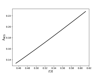
Figure 3: This non-interesting straight line (within the accuracy of the numerical calculation) represents the relation between the BCS coupling constant $\lambda$ defined in Eq. (15) accepting common $J_{sd}$ given in Table 2 for all cuprates and the ratio of the tight binding parameters $t^{\prime}/t$ calculated in Eq. (30) where Eq. (8) is substituted. It is well-known according to Eq. (14) that $\lambda$ has the main influence on the critical temperature $T_{c}$. The complicated integral representing $\langle\chi^{2}\rangle\rho_{\mathrm{{}_{F}}}$ with analytical expression Eq. (4) substituted in the Fermi contour averaging Eq. (11) gives little hope for an analytical solution. In such a way we have only the graphical solution that the BCS coupling constant $\lambda$ is in good approximation linear function of the $t^{\prime}/t$ parameter determining the shape of the Fermi surface; for both variables we have derived complicated explicit expressions Eq. (30) and Eq. (14) exact in the used LCAO approximation for electronic the band structure.

We are surprised that after almost lethal dose of tedious elementary calculation we have obtained an unexpected approximate linear dependence. This linear dependence between $\langle\chi^{2}\rangle\rho_{\mathrm{{}_{F}}}$ and $t^{\prime}/t$ is a highly nontrivial (for us) result which gives the final explanation of Pavarini et al. [20] correlation from Fig. 2. We have to look it in the correct variables: the BCS coupling constant $\lambda$ is a linear function of $t^{\prime}/t$ according to Fig. 3. Then $\ln T_{c,\,\mathrm{max}}$ is a linear function of $t^{\prime}/t$ according to re-drawn experimental correlation represented in Fig. 2. According to the BCS result for the critical temperature Eq. (14) we observe just a correlation between $\ln T_{c,\,\mathrm{max}}$ and the reciprocal BCS coupling constant $1/\lambda$ which is determined mainly by the relative position of the Cu4$s$ level with respect of Cu3$d_{x^{2}-y^{2}}$. In the tight binding modeling by Honerkamp and Rice [40] and Sarasua [41] was found that $t^{\prime}/t$ ratio is favorable for pairing, but in the present study we reveal that this ratio is determined by the Cu4$s$ level.

In order avoid misunderstandings we have to clarify that $T_{c,\,\mathrm{max}}$ depends also on doping or chemical potential. But the Pavarini et al. [20] correlations are just for optimally doped cuprates for which the relative area of the hole pocket is almost the same and this optimal doping fixes the chemical potential or Fermi level. We have to add that interesting physics of underdoped cuprates is often irrelevant for the optimally doped. Optimally doped means doping level for which the critical temperature is maximal for the corresponding compound. However high-$T_{c}$ cuprates attracted big attention just because their high critical temperature and the purpose of our study is to reveal what is the pairing mechanism leading to this high critical temperature at optimal doping.

V Conclusion

Let us compare the results for Kondo interaction with the results of phonon model, see for example the recent study by Marsiglio [42]. Our Eq. (15) and our Fig. 2 are very similar to [42, Eq. (26) and Fig. 1 and Fig. 4] however every model for cuprate superconductivity has its own parameters of the theory which are difficult to be calculated ab initio. For example $J_{sd}$ exchange constant and electron phonon coupling constant. We are disappointed from the phonon model because its unable to derive within the Pavarini [20] correlations and gap anisotropy but the game has not finished yet. If the theory has parameters determined by the fit to an experiment some dimensionless parameters in equalities have to be checked. In our case for applicability of the BCS approach we have to check whether $T_{c,\,\mathrm{max}}\ll E_{\mathrm{C}}$.

There are many models for the CuO₂ superconductivity but why the critical temperature in different cuprates is so different? How to determine the parameters of these effective Hamiltonians? And how to derive microscopically the influence of the Cu4$s$ level on their parameters? Superconducting phase transition is determined by the pairing interaction and if the position of the Cu4$s$ level has big influence on $T_{c,\,\mathrm{max}}$ this is a hint that the Cu4$s$ state is important ingredient of the pairing interaction, in our case Eq. (5).

The passed decades have revealed that high-$T_{c}$ materials posses all properties of the BCS superconductors: charge of Cooper pairs, band structure, superconducting gap etc. For Kondo interaction applied to the CuO₂ plane the pairing function is factorizable. For factorizable pairing the BCS scheme is just application of trial function approach. Trial function approach has much broader region of applicability than weak coupling regime $\lambda\ll 1$. For his theory of anisotropic gap superconductors Pokrovsky derived the factorizable pairing interaction within the weak coupling approximation, but this condition is not necessary for cuprates. In other words the Pokrovsky theory for anisotropic gap superconductor is applicable for exchange pairing in cuprates even for moderate coupling constants, say $\lambda\sim 1/2$. However, the main result of the present study is not the BCS estimation of $T_{c,\,\mathrm{max}}$, but the qualitative result that only Kondo s-d interaction considered as a pairing mechanism explains the well-known experimentally observed correlation between the critical temperature of the optimally doped cuprates and the shape of the Fermi contour.

Performed analysis of this unexplained correlation, see Fig. 2, reveals that the BCS pairing theory is even with acceptable accuracy quantitatively applicable to explain the main property of HTS cuprates – their high temperature $T_{c,\,\mathrm{max}}$ at optimal doping. Due to lack of alternative explanation cf. Ayres, Katsnelson and Hussey [43] we arrive at the conclusion that long sought mechanism of HTS is already found – the well-known Kondo exchange interaction applied to the conduction band charge carriers.

Author contributions

All authors have equally contributed to the writing of the manuscript, programming, making of figures and experimental data processing.

Data availability statement

The data that support the findings of this study are available upon reasonable request from the authors.

References

- Bednorz and Müller [1986] J. G. Bednorz and K. A. Müller, Possible high Tc superconductivity in the Ba-La-Cu-O system, Zeitschrift fur Physik B Cond. Matt. 64, 189 (1986).
- M. B. Brodsky, G. W. Crabtree, B. D. Dunlap, R. P. Griessen, S. Maekawa, Yu. A. Osipyan, H. R. Ott, S. Tanaka [1988] M. B. Brodsky, G. W. Crabtree, B. D. Dunlap, R. P. Griessen, S. Maekawa, Yu. A. Osipyan, H. R. Ott, S. Tanaka, ed., Procs. Int. Conf. on High Temperature Superconductors and Materials and Mechanisms of Superconductivity, Vol. Phys. C 153–155 (North Holland, Amsterdam, 1988).
- Emery [1987] V. J. Emery, Theory of High- Superconductivity in Oxides, Phys. Rev. Lett. 58, 2794 (1987).
- Monthoux et al. [1991] P. Monthoux, A. V. Balatsky, and D. Pines, Toward a theory of high-temperature superconductivity in the antiferromagnetically correlated cuprate oxides, Phys. Rev. Lett. 67, 3448 (1991).
- Anderson [1987] P. W. Anderson, The Resonating Valence Bond State in La2CuO4 and Superconductivity, Science 235, 1196 (1987).
- Varma et al. [1987] C. Varma, S. Schmitt-Rink, and E. Abrahams, Charge transfer excitations and superconductivity in “ionic” metals, Solid State Commun. 62, 681 (1987).
- Zhang and Rice [1988] F. C. Zhang and T. M. Rice, Effective Hamiltonian for the superconducting Cu oxides, Phys. Rev. B 37, 3759 (1988).
- Anderson [1997] P. W. Anderson, The Theory of Superconductivity in the High-S Cuprate Superconductors (Princeton University Press, Princeton, New Jersey, 1997).
- Lee et al. [2006] P. A. Lee, N. Nagaosa, and X.-G. Wen, Doping a Mott insulator: Physics of high-temperature superconductivity, Rev. Mod. Phys. 78, 17 (2006), arXiv:cond-mat/0410445 [cond-mat.str-el] .
- Keimer et al. [2015] B. Keimer, S. A. Kivelson, M. R. Norman, S. Uchida, and J. Zaanen, From quantum matter to high-temperature superconductivity in copper oxides, Nature (London) 518, 179 (2015).
- Spałek et al. [2022] J. Spałek, M. Fidrysiak, M. Zegrodnik, and A. Biborski, Superconductivity in high- and related strongly correlated systems from variational perspective: Beyond mean field theory, Phys. Rep. 959, 1 (2022).
- Arovas et al. [2022] D. P. Arovas, E. Berg, S. A. Kivelson, and S. Raghu, The Hubbard Model, Ann. Rev. Condens. Matter Phys. 13, 239 (2022).
- Presland et al. [1991] M. Presland, J. Tallon, R. Buckley, R. Liu, and N. Flower, General trends in oxygen stoichiometry effects on in Bi and Tl superconductors, Physica C: Supercond. 176, 95 (1991).
- Dimitrov et al. [2011] Z. Dimitrov, S. Varbev, K. Omar, A. Stefanov, E. Penev, and T. Mishonov, Correlation between and the Cu Level Reveals the Mechanism of High-Temperature Superconductivity, Bulg. J. Phys. 38, 106 (2011), arXiv:1103.2966 [cond-mat.supr-con] .
- Mishonov and Penev [2010] T. M. Mishonov and E. S. Penev, Theory of High Temperature Superconductivity. A Conventional Approach (World Scientific, New Jersey, 2010).
- Andersen et al. [1995] O. Andersen, A. Liechtenstein, O. Jepsen, and F. Paulsen, LDA energy bands, low-energy hamiltonians, , , , and , J. Phys. Chem. Solids 56, 1573 (1995), Procs. Conf. Spectroscopies in Novel Superconductors.
- Andersen et al. [1996] O. K. Andersen, S. Y. Savrasov, O. Jepsen, and A. I. Liechtenstein, Out-of-plane instability and electron-phonon contribution to - and -wave pairing in high-temperature superconductors; LDA linear-response calculation for doped CaCuO2 and a generic tight-binding model, J. Low Temp. Phys. 105, 285 (1996).
- Röhler [2000a] J. Röhler, Plane dimpling and Cu hybridization in YBa2Cu3Ox, Physica B: Cond. Matter 284-288, 1041 (2000a).
- Röhler [2000b] J. Röhler, The underdoped-overdoped transition in YBa2Cu3Ox, Physica C: Supercond. and Appl. 341-348, 2151 (2000b).
- Pavarini et al. [2001] E. Pavarini, I. Dasgupta, T. Saha-Dasgupta, O. Jepsen, and O. K. Andersen, Band-Structure Trend in Hole-Doped Cuprates and Correlation with , Phys. Rev. Lett. 87, 047003 (2001).
- Damascelli et al. [2003] A. Damascelli, Z. Hussain, and Z.-X. Shen, Angle-resolved photoemission studies of the cuprate superconductors, Rev. Mod. Phys. 75, 473 (2003).
- Damascelli [2004] A. Damascelli, Probing the Electronic Structure of Complex Systems by ARPES, Phys. Scr. 2004, 61 (2004).
- Yu et al. [2020] T. Yu, C. E. Matt, F. Bisti, X. Wang, T. Schmitt, J. Chang, H. Eisaki, D. Feng, and V. N. Strocov, The relevance of ARPES to high-Tc superconductivity in cuprates, npj Quantum Mater. 5, 46 (2020).
- Sobota et al. [2021] J. A. Sobota, Y. He, and Z.-X. Shen, Angle-resolved photoemission studies of quantum materials, Rev. Mod. Phys. 93, 025006 (2021).
- Zonno et al. [2021] M. Zonno, F. Boschini, and A. Damascelli, Time-resolved ARPES on cuprates: Tracking the low-energy electrodynamics in the time domain, J. Electron Spectrosc. 251, 147091 (2021), arXiv:2106.11316 [cond-mat.supr-con] .
- Zhang et al. [2014] W. Zhang, C. Hwang, C. L. Smallwood, T. L. Miller, G. Affeldt, K. Kurashima, C. Jozwiak, H. Eisaki, T. Adachi, Y. Koike, D.-H. Lee, and A. Lanzara, Ultrafast quenching of electron-boson interaction and superconducting gap in a cuprate superconductor, Nat. Comm. 5, 10.1038/ncomms5959 (2014), arXiv:1410.1615 [cond-mat.supr-con] .
- Nakayama et al. [2007] K. Nakayama, T. Sato, K. Terashima, H. Matsui, T. Takahashi, M. Kubota, K. Ono, T. Nishizaki, Y. Takahashi, and N. Kobayashi, Bulk and surface low-energy excitations in studied by high-resolution angle-resolved photoemission spectroscopy, Phys. Rev. B 75, 014513 (2007).
- Okawa et al. [2010] M. Okawa, K. Ishizaka, H. Uchiyama, H. Tadatomo, T. Masui, S. Tajima, X.-Y. Wang, C.-T. Chen, S. Watanabe, A. Chainani, T. Saitoh, and S. Shin, Bulk-sensitive laser-ARPES study on the cuprate superconductor YBa2Cu3O7-δ, Physica C: Supercond. and Appl. 470, S62 (2010), Procs. 9th Int. Conf. on Materials and Mechanisms of Superconductivity.
- Campuzano [2018] J. C. Campuzano, Abrikosov and the path to understanding high- superconductivity, Low Temp. Phys. 44, 506 (2018).
- Mishonov et al. [2022a] T. M. Mishonov, N. I. Zahariev, H. Chamati, and A. M. Varonov, Hot spots along the Fermi contour of high- cuprates explained by - exchange interaction, SN Appl. Sci. 4, 242 (2022a), arXiv:2208.00936 [cond-mat.supr-con] .
- Mishonov et al. [2021] T. M. Mishonov, N. I. Zahariev, and A. M. Varonov, Hot and cold spots along the Fermi contour of high- cuprates in the framework of Shubin-Kondo-Zener - exchange interaction (2021), arXiv:2111.06716 [cond-mat.supr-con] .
- Mishonov et al. [2022b] T. M. Mishonov, N. I. Zahariev, H. Chamati, and A. M. Varonov, Possible zero sound in layered perovskites with ferromagnetic - exchange interaction, SN Appl. Sci. 4, 228 (2022b), arXiv:2208.00938 [cond-mat.supr-con] .
- Wei et al. [1998] J. Y. T. Wei, C. C. Tsuei, P. J. M. van Bentum, Q. Xiong, C. W. Chu, and M. K. Wu, Quasiparticle tunneling spectra of the high- mercury cuprates: Implications of the -wave two-dimensional van Hove scenario, Phys. Rev. B 57, 3650 (1998).
- Schrieffer [2007] J. R. Schrieffer, ed., Handbook of High-Temperature Superconductivity: Theory and Experiment (Springer-Verlag, New York, 2007).
- Pokrovskii [1961] V. L. Pokrovskii, Thermodynamics of Anisotropic Superconductors, J. Exp. Theor. Phys. 13, 447 (1961), ZhETF 40(2), 641 Aug (1961), http://www.jetp.ras.ru/cgi-bin/r/index/r/40/2/p641?a=list (in Russian).
- Lifshitz and Pitaevskii [1980] E. M. Lifshitz and L. P. Pitaevskii, Statistical Physics. Part 2, Landau-Lifshitz Course of Theoretical Physics, Vol. 9 (Pergamon, New York, 1980).
- Won and Maki [1994] H. Won and K. Maki, -wave superconductor as a model of high- superconductors, Phys. Rev. B 49, 1397 (1994).
- Johnson et al. [2001] P. D. Johnson, T. Valla, A. V. Fedorov, Z. Yusof, B. O. Wells, Q. Li, A. R. Moodenbaugh, G. D. Gu, N. Koshizuka, C. Kendziora, S. Jian, and D. G. Hinks, Doping and Temperature Dependence of the Mass Enhancement Observed in the Cuprate , Phys. Rev. Lett. 87, 177007 (2001), arXiv:cond-mat/0102260 [cond-mat.supr-con] .
- Mishonov et al. [1996] T. M. Mishonov, R. K. Koleva, I. N. Genchev, and E. S. Penev, Quantum chemical calculation of oxygen-oxygen electron hopping amplitude - first principles evaluation of conduction bandwidth in layered cuprates, Czech J. Phys. 46, 2645 (1996).
- Honerkamp and Maurice Rice [2003] C. Honerkamp and T. Maurice Rice, Single band model for the unconventional superconductivity in both cuprates and ruthenates, Physica C: Supercond. 388-389, 11 (2003), Procs. 23rd Int. Conf. Low Temp. Phys. (LT23).
- Sarasua [2011] L. G. Sarasua, Superconductivity from strong repulsive interactions in the two-dimensional Hubbard model, Phys. Scr. 84, 045706 (2011).
- Marsiglio [2018] F. Marsiglio, Eliashberg theory in the weak-coupling limit, Phys. Rev. B 98, 024523 (2018), arXiv:1807.04907 [cond-mat.supr-con] .
- Ayres et al. [2022] J. Ayres, M. I. Katsnelson, and N. E. Hussey, Superfluid density and two-component conductivity in hole-doped cuprates, Front. Phys. 10, 1021462 (2022).