Fluctuation without dissipation: Microcanonical Langevin Monte Carlo

Abstract

Stochastic sampling algorithms such as Langevin Monte Carlo are inspired by physical systems in a heat bath. Their equilibrium distribution is the canonical ensemble given by a prescribed target distribution, so they must balance fluctuation and dissipation as dictated by the fluctuation-dissipation theorem. In contrast to the common belief, we show that the fluctuation-dissipation theorem is not required because only the configuration space distribution, and not the full phase space distribution, needs to be canonical. We propose a continuous-time Microcanonical Langevin Monte Carlo (MCLMC) as a dissipation-free system of stochastic differential equations (SDE). We derive the corresponding Fokker-Planck equation and show that the stationary distribution is the microcanonical ensemble with the desired canonical distribution on configuration space. We prove that MCLMC is ergodic for any nonzero amount of stochasticity, and for smooth, convex potentials, the expectation values converge exponentially fast. Furthermore, the deterministic drift and the stochastic diffusion separately preserve the stationary distribution. This uncommon property is attractive for practical implementations as it implies that the drift-diffusion discretization schemes are bias-free, so the only source of bias is the discretization of the deterministic dynamics. We applied MCLMC on a lattice $\phi^{4}$ model, where Hamiltonian Monte Carlo (HMC) is currently the state-of-the-art integrator. For the same accuracy, MCLMC converges 12 times faster than HMC on an $8\times 8$ lattice. On a $64\times 64$ lattice, it is already 32 times faster. The trend is expected to persist to larger lattices, which are of particular interest, for example, in lattice quantum chromodynamics.

I Introduction

The dynamics of a particle with location $\bm{x}(t)$, momentum $\bm{\Pi}(t)$, and the Hamiltonian function $H(\bm{x},\,\bm{\Pi})=\frac{1}{2}|\bm{\Pi}|^{2}+S(\bm{x})$ is described by the Hamiltonian equations, which is a deterministic system of ordinary differential equations (ODE) for the phase space variables $\bm{z}=(\bm{x},\bm{\Pi})$. Langevin dynamics additionally models microscopic collisions with a heat bath by introducing damping and the diffusion process giving rise to a set of Stochastic Differential Equations (SDE). Damping and diffusion are tied together by the fluctuation-dissipation theorem, ensuring that the probability distribution $\rho_{t}(\bm{z})$ converges to the canonical ensemble $\propto\exp[-H(\bm{z})]$ on the phase space. The marginal configuration space distribution is then also canonical $\rho(\bm{x})\propto\exp[-S(\bm{x})]$. The time evolution of the density is governed by the Liouville equation for Hamiltonian dynamics and by the Fokker-Planck equation for Langevin dynamics, both of which are deterministic partial differential equations (PDE).

Hamiltonian dynamics, supplemented by occasional Gaussian momentum resampling, converges to the canonical distribution on the phase space, so both Langevin and Hamiltonian dynamics can be used to sample from an arbitrary distribution $\rho(\bm{x})\propto\exp[-S(\bm{x})]$, provided that we can compute the potential gradient $\nabla S(\bm{x})$ needed to simulate the dynamics. The resulting algorithms are called (underdamped) Langevin Monte Carlo (LMC) (e.g. Leimkuhler and Matthews (2015)) and Hamiltonian (also called Hybrid) Monte Carlo (HMC) Duane et al. (1987). Both LMC and HMC have been applied in the context of high dimensional Monte Carlo Markov Chain (MCMC) sampling, such as Bayesian posteriors, field theory, statistical physics, etc. In high-dimensional settings, these gradient-based methods are vastly more efficient than gradient-free MCMC, such as Metropolis-Hastings Metropolis et al. (2004). Metropolis-Hastings adjustment is however used for acceptance or rejection of HMC trajectory and related procedures exist for LMC as well Riou-Durand and Vogrinc (2022).

An interesting question is what is the complete framework of possible ODE/SDE whose equilibrium solution corresponds to the canonical target density $\rho(\bm{x})\propto\exp[-S(\bm{x})]$. It has been argued (Ma et al., 2015) that the complete framework is given by a general form of the drift term $B(\bm{z})=[D(\bm{z})+Q(\bm{z})]\nabla H(\bm{z})+\Gamma(\bm{z})$, where $H(\bm{z})$ is the Hamiltonian, $D(\bm{z})$ is positive definite diffusion matrix and $Q(\bm{z})$ is skew-symmetric matrix. $\Gamma(\bm{z})$ is specified by derivatives of $D(\bm{z})$ and $Q(\bm{z})$. This framework implicitly assumes that the equilibrium distribution is canonical on the phase space, $\rho(\bm{z})\propto\exp[-H(\bm{z})]$, after which the momentum can be integrated out for Hamiltonians with separable kinetic and potential energies.

In general, however, we only need to require the marginal $\bm{x}$ distribution to be canonical, $\rho(\bm{x})\propto\exp[-S(\bm{x})]$, giving rise to the possibility of additional formulations for which the stationary distribution matches the target distribution, but without the phase space distribution being canonical. One such example is the Microcanonical Hamiltonian Monte Carlo (Ver Steeg and Galstyan, 2021; Robnik et al., 2022) (MCHMC), where the energy is conserved throughout the process, and a suitable choice of the kinetic energy and momentum bounces enforces the correct marginal configuration space distribution.

The purpose of this paper is to explore MCHMC in the continuous-time limit, with and without diffusion. In section II we derive the Liouville equation for continuous deterministic dynamics directly from the ODE, and show that its stationary solution is the target distribution. In section III we extend from ODE to an SDE, giving rise to continuous Microcanonical Langevin (MCLMC) dynamics. In contrast to the standard Langevin dynamics, the energy conservation leads to dynamics that does not have a velocity damping term associated with the stochastic term, such that the noise is energy conserving. We derive the associated Fokker-Planck equation and show its stationary solution is the same as for the Liouville equation. In section V we prove that SDE is ergodic and in section VI we demonstrate that it is also geometrically ergodic for smooth, log-convex target distributions.

In section VII we apply MCLMC to study the statistical $\phi^{4}$ field theory and compare it with Hamiltonian Monte Carlo.

II Deterministic dynamics

The continuous time evolution of a particle in the Microcanonical Hamiltonian Monte Carlo between the bounces is given by the ODE (Robnik et al., 2022; Ver Steeg and Galstyan, 2021)

$$\dot{\bm{x}} =\bm{u}$$ (1)

$$\dot{\bm{u}} =P(\bm{u})\bm{f}(\bm{x}),$$

where $\bm{x}$ is the position of a particle in the configuration space and $\bm{u}$ is its velocity. We have introduced the projector $P(\bm{u})=I-\bm{u}\bm{u}^{T}$ and we introduced the force $\bm{f}(\bm{x})=-\nabla S(\bm{x})/(d-1)$. The force in Robnik et al. (2022); Ver Steeg and Galstyan (2021) was defined with a factor of $d$ rather than $d-1$, which required weights. These weights are eliminated with the new formulation here.

The dynamics preserves the norm of $\bm{u}$ if we start with $\bm{u}\cdot\bm{u}=1$,

$$\frac{d}{dt}(\bm{u}\cdot\bm{u})=2\bm{u}\cdot\dot{\bm{u}}=\bm{u}\cdot P(\bm{u})\bm{f}=(1-\bm{u}\cdot\bm{u})(\bm{u}\cdot\bm{f})=0,$$ (2)

so the particle is confined to the $2d-1$ dimensional manifold $\mathcal{M}=\mathbb{R}^{d}\times S^{d-1}$, i.e. the velocity is defined on a sphere of unit radius. We will denote the points on $\mathcal{M}$ by $\bm{z}$.

Equivalently, the dynamics of Equation (1) can be described by the flow on the manifold, which is a 1-parametrical family of maps from the manifold onto itself $\varphi_{t}:\mathcal{M}\xrightarrow[]{}\mathcal{M}$, such that $\varphi_{t}(\bm{z})$ is the solution of Equation (1) with the initial condition $\bm{z}$. The flow induces the drift vector field $B(\bm{z})$, which maps scalar observables on the manifold $\mathcal{O}(\bm{z})$ to their time derivatives under the flow,

$$B(\bm{z})(\mathcal{O})=\frac{d}{dt}\mathcal{O}\big{(}\varphi_{t}(\bm{z})\big{)}|_{t=0}.$$ (3)

We will be interested in the evolution of the probability density distribution of the particle under the flow. In differential geometry, the density is described by a volume form, which is a differential $(2d-1)$-form,

$$\widehat{\rho}(\bm{z})=\rho(\bm{z})\,dz^{1}\wedge dz^{2}\wedge...\,dz^{2d-1}.$$ (4)

Suppose we are given the volume form $\widehat{\rho}_{t}$ at some time $t$. Formally, we can translate it in time by applying the push-forward map $\varphi_{s*}$, $\widehat{\rho}_{t+s}=\varphi_{s*}\widehat{\rho}_{t}$. The infinitesimal form of the above equation gives us the differential equation for the density:

$$\frac{d}{dt}\widehat{\rho}_{t} =\frac{d}{ds}\big{(}\varphi_{s*}\widehat{\rho}_{t}\big{)}|_{s=0}=\frac{d}{ds}\big{(}\varphi_{-s}^{*}\widehat{\rho}_{t}\big{)}|_{s=0}\equiv-\mathcal{L}_{B}\widehat{\rho}_{t}$$ (5)

$$=-\big{(}\mathrm{div}_{\widehat{\rho}_{t}}B\big{)}\widehat{\rho}_{t},$$

which is also known as the Liouville equation. Here, $\varphi^{*}_{-s}=\varphi_{s*}$ is the pull-back map, $\mathcal{L}_{B}$ is the Lie derivative along the drift vector field $B$ and $\mathrm{div}$ is the divergence. This is the continuity equation for the probability in the language of differential geometry.

The Liouville equation in coordinates is

$$\dot{\rho}(\bm{z})=-\nabla\cdot\big{(}\rho B\big{)}\equiv-\sum_{i=1}^{2d-1}\frac{\partial}{\partial z^{i}}\big{(}\rho(\bm{z})B^{i}(\bm{z})\big{)}$$ (6)

We will work in the Euclidean coordinates $\{x^{i}\}_{i=1}^{d}$ on the configuration space and spherical coordinates $\{\vartheta^{\mu}\}_{\mu=1}^{d-1}$ for the velocities on the sphere, such that the manifold is parametrized by $\bm{z}=(\bm{x},\bm{\vartheta})$. We will adopt the Einstein summation convention and use the Latin letters ($i$, $j$, …) to indicate the sum over the Euclidean coordinates and the Greek letters ($\mu$, $\nu$, …) for the sum over the spherical coordinates. The spherical coordinates are defined by the inverse transformation,

$$u_{1}= \cos\vartheta^{1},$$ (7)

$$u_{2}= \sin\vartheta^{1}\cos\vartheta^{2}$$

$$\vdots\,$$

$$u_{d-1}= \sin\vartheta^{1}\cdots\sin\vartheta^{d-2}\cos\vartheta^{d-1}$$

$$u_{d}= \sin\vartheta^{1}\cdots\sin\vartheta^{d-2}\sin\vartheta^{d-1},$$

which automatically ensures $\bm{u}\cdot\bm{u}=1$. The metric on the sphere in the spherical coordinates is

$$g_{\mu\nu}=\frac{\partial u_{k}}{\partial\vartheta^{\mu}}\frac{\partial u_{k}}{\partial\vartheta^{{\nu}}}=\mathrm{Diag}[1,\,\sin^{2}(\vartheta^{1}),\,\sin^{2}(\vartheta^{1})\sin^{2}(\vartheta^{2}),\,...]_{ij},$$ (8)

and the volume element is $\sqrt{g}=\mathrm{det}g_{\mu\nu}^{1/2}=\Pi_{k=1}^{d-2}(\sin\vartheta^{k})^{d-1-k}$. The drift vector field is

$$B=u_{i}(\bm{\vartheta})\frac{\partial}{\partial x^{i}}+\partial^{\mu}(\bm{u}\cdot\bm{f}(\bm{x}))\frac{\partial}{\partial\vartheta^{\mu}},$$ (9)

where the second term results from $B_{\nu}=\frac{\partial u_{i}}{\partial\vartheta^{\nu}}P_{ij}f_{j}=\frac{\partial u_{i}}{\partial\vartheta^{\nu}}f_{i}$.

Theorem 1.

The stationary solution of Liouville equation (6) is

$$\rho_{\infty}\propto e^{-S(\bm{x})}\sqrt{g(\bm{\vartheta})}.$$ (10)

Proof.

Inserting $\rho_{\infty}$ in the Liouville equation (6) gives

$$\dot{\rho}_{\infty}=-\bm{u}\cdot\partial_{\bm{x}}\rho_{\infty}-\frac{1}{\sqrt{g}}\partial_{\mu}\big{(}\sqrt{g}B^{\mu}\big{)}\rho_{\infty}.$$

The first term is $\bm{u}\cdot\partial_{\bm{x}}\rho_{\infty}=(d-1)\bm{u}\cdot\bm{f}\rho_{\infty}$. The second term transforms as a scalar under the transformations of the spherical coordinates. We can use this to simplify the calculation: at each fixed $\bm{x}$ we will pick differently oriented spherical coordinates, such that $\vartheta^{1}=0$ always corresponds to the direction of $\bm{f}(\bm{x})$ and $f_{i}=\delta_{1i}|\bm{f}|$. We then compute $B_{\mu}=(\partial_{\mu}u_{1})|\bm{f}|=-\sin\vartheta^{1}\delta_{1\mu}|\bm{f}|$, so

$$\frac{1}{\sqrt{g}}\partial_{\mu}\big{(}\sqrt{g}B^{\mu}\big{)}=\frac{-|\bm{f}|}{\sin^{d-2}\vartheta^{1}}\frac{\partial}{\partial\vartheta^{1}}\sin^{d-1}\vartheta^{1}$$

$$=-(d-1)|\bm{f}|\cos\vartheta^{1}=-(d-1)\bm{u}\cdot\bm{f}.$$

The last expression transforms as a scalar with respect to transformations on the sphere and is therefore valid in all coordinate systems, in particular, in the original one. Combining the two terms gives $\dot{\rho}_{\infty}=0$, completing the proof. ∎

III Stochastic dynamics

In Robnik et al. (2022) it was proposed that adding a random perturbation to the momentum direction after each step of the discretized deterministic dynamics boosts ergodicity, but the continuous-time version was not explored. Here, we consider a continuous-time analog and show this leads to Microcanonical Langevin SDE for the particle evolution and to Fokker-Planck equation for the probability density evolution. We promote the deterministic ODE of Equation (1) to the following Microcanonical Langevin SDE:

$$d\bm{x} =\bm{u}dt$$ (11)

$$d\bm{u} =P(\bm{u})\bm{f}(\bm{x})dt+\eta P(\bm{u})d\bm{W}.$$

Here, $\bm{W}$ is the Wiener process, i.e. a vector of random noise variables drawn from a Gaussian distribution with zero mean and unit variance, and $\eta$ is a free parameter. The last term is the standard Brownian motion increment on the sphere, constructed by an orthogonal projection from the Euclidean $\mathbb{R}^{d}$, as in Elworthy (1998a).

More formally, we may write Equation (11) as a Stratonovich degenerate diffusion on the manifold (Elworthy, 1998b; Baxendale, 1991; Kliemann, 1987),

$$d\bm{z}=B(\bm{z})dt+\sum_{i=1}^{d}\sigma_{i}(\bm{z})\circ dW_{i},$$ (12)

where $W_{i}$ are independent $\mathbb{R}$-valued Wiener processes and $\sigma_{i}$ are vector fields, in coordinates expressed as

$$\sigma_{i}(\bm{\vartheta})=g^{\mu\nu}(\bm{\vartheta})\frac{\partial u_{i}}{\partial\vartheta^{\nu}}(\bm{\vartheta})\frac{\partial}{\partial\vartheta^{\mu}}.$$ (13)

With the addition of the diffusion term, the Liouville equation (6) is now promoted to the Fokker-Planck equation (Elworthy, 1998a),

$$\dot{\rho}=-\nabla\cdot(\rho B)+\frac{\eta^{2}}{2}\widehat{\nabla}^{2}\rho,$$ (14)

where $\widehat{\nabla}^{2}=\nabla^{\mu}\nabla_{\mu}$ is the Laplace-Beltrami operator on the sphere and $\nabla_{\mu}$ is the covariant derivative on the sphere. In coordinates, the Laplacian can be computed as $\frac{1}{\sqrt{g}}\partial_{\mu}\big{(}\sqrt{g}\partial^{\mu}\rho\big{)}$.

Theorem 2.

The distribution $\rho_{\infty}$ of Equation (10) is a stationary solution of the Fokker-Planck equation (14) for any value of $\eta$.

Proof.

Upon inserting $\rho_{\infty}$ into the right-hand-side of the Fokker-Planck equation, the first term vanishes by Theorem 1. The second term also vanishes,

$$\widehat{\nabla}^{2}\rho_{\infty}\propto\nabla^{\mu}\nabla_{\mu}\sqrt{g}e^{-S(\bm{x})}=e^{-S(\bm{x})}\nabla^{\mu}\nabla_{\mu}\sqrt{g}=0,$$

since the covariant derivative of the metric determinant is zero. This completes the proof. ∎

IV Discretization

Consider for a moment Equation (11) with only the diffusion term on the right-hand-side. This SDE describes the Brownian motion on the sphere and the identity flow on the $\bm{x}$-space (Elworthy, 1998a). Realizations from the Brownian motion on the sphere can be generated exactly (Li and Erdogdu, 2020). Let us denote by $\psi^{\eta}_{s}$ the corresponding density flow map, such that $\psi^{\eta}_{s}[\rho_{t}]=\rho_{t+s}$. The flow of the full SDE (11) can then be approximated at discrete times $\{n\epsilon\}_{n=0}^{\infty}$ by the Euler-Maruyama scheme (Øksendal and Øksendal, 2003):

$$\rho_{(n+1)\epsilon}=\psi^{\eta}_{\epsilon}[\varphi_{\epsilon*}\,\rho_{n\epsilon}].$$ (15)

For a generic SDE, this approximation leads to bias in the stationary distribution. This is however not the case in MCLMC:

Theorem 3.

The distribution $\rho_{\infty}$ of Equation (10) is preserved by the Euler-Maruyama scheme (15) for any value of $\eta$.

Proof.

The deterministic push forward map preserves $\rho_{\infty}$ by the Theorem 1. The Fokker-Planck equation for the stochastic-only term is $\dot{\rho}=\frac{\eta^{2}}{2}\widehat{\nabla}\rho$ which preserves $\rho_{\infty}$ by the Theorem 2. ∎

In the standard Langevin equation, the fluctuation term is accompanied by a dissipation term, and the strength of both is controlled by damping coefficient. The deterministic and stochastic parts do not preserve the stationary distribution separately. In contrast, for MCLMC an exact deterministic ODE integrator would remain exact with SDE, so the integration scheme for the deterministic dynamics is the only bias source.

Furthermore, in the discrete scheme (15) it is not necessary to have the Brownian motion on the sphere as a stochastic update in order to have $\rho_{\infty}$ as a stationary distribution. In fact, any discrete stochastic process on the sphere, which has the uniform distribution as the stationary distribution will do, for example the one used in Robnik et al. (2022).

V Ergodicity

We have established that $\rho_{\infty}$ is the stationary distribution of the MCLMC SDE. Here we demonstrate the uniqueness of the stationary distribution.

Let’s define $\mathcal{S}(\bm{z})=\{B(\bm{z}),\sigma_{1}(\bm{z}),\sigma_{2}(\bm{z}),\ldots\sigma_{d}(\bm{z})\}$. The Hörmander’s condition (Leimkuhler and Matthews, 2015) is satisfied at $\bm{z}\in\mathcal{M}$ if the smallest Lie algebra containing $\mathcal{S}(\bm{z})$ and closed under $v\mapsto[B,v]$ is the entire tangent space $T_{\bm{z}}(\mathcal{M})$. Here $[\cdot,\cdot]$ is the Lie bracket, in coordinates $[X,Y]=X^{i}\partial_{i}Y^{k}\partial_{k}-Y^{i}\partial_{i}X^{k}\partial_{k}$.

Lemma 1.

(Hörmander’s property) MCLMC SDE satisfies the Hörmander’s condition for all $\bm{z}\in\mathcal{M}$.

Proof.

Fix some $\bm{z}=(\bm{x},\bm{u})$. The tangent space at $\bm{z}$ is a direct sum $T_{\bm{z}}(\mathcal{M})=T_{\bm{x}}(\mathbb{R}^{d})\oplus T_{\bm{u}}(S^{d-1})$. $\sigma_{i}$ span $T_{\bm{u}}(S^{d-1})$ by construction: they were obtained by passing the basis of $\mathbb{R}^{d}$ thought the orthogonal projection, $P(\bm{u})$, which has rank $d-1$. For convenience we may further decompose $T_{\bm{x}}(\mathbb{R}^{d})=U\oplus U^{\perp}$, where $U=\{\lambda\bm{u}|\lambda\in\mathbb{R}\}$ is the space spanned by $\bm{u}$ and $U^{\perp}$ is its orthogonal complement. We can write $B=B_{x}+B_{u}$, such that $B_{x}\in T_{\bm{x}}(\mathbb{R}^{d})$ and $B_{u}\in T_{\bm{u}}(S^{d-1})$, see also Equation (9). $B_{x}=u_{i}\partial_{x^{i}}$ spans $U$, so we are left with covering $U^{\perp}$. $[B_{u},\sigma_{i}]\in T_{\bm{u}}(S^{d-1})$, so it does not interest us anymore. However,

$$[B_{x},\,\sigma_{i}]=-\sigma_{i}(B_{x})=g^{\mu\nu}\frac{\partial u_{i}}{\partial\vartheta^{\mu}}\frac{\partial u_{j}}{\partial\vartheta^{\nu}}\partial_{j},$$

so $[B_{x},\,\sigma_{i}]$ span $U^{\perp}$, completing the proof. ∎

Lemma 2.

(Path accessibility of points): For every two points $\bm{z}_{i},\bm{z}_{f}\in\mathcal{M}$ there exists a continuous path $\gamma:[0,T]\rightarrow\mathcal{M}$, $\gamma(0)=\bm{z}_{i}$, $\gamma(T)=\bm{z}_{f}$ and values $0=t_{0}<t_{1}<\cdots<t_{N}=T$ with a corresponding sequence of vectors $v_{n}\in\mathcal{S}$, such that for each $0\leq n<N$, $\dot{\gamma}(t)=v_{n}(\gamma(t))$ for $t_{n}<t<t_{n+1}$.

Proof.

Starting at $\bm{z}_{i}$, we will reach $\bm{z}_{f}$ in three stages. In stage I, we will use $\sigma_{i}$ to reorient $\bm{u}_{i}$ to the desired direction $\bar{\bm{u}}$ (as determined by the stage II). In stage II we will then follow $B$ to reach the final destination $\bm{x}_{f}$ in the configuration space. In stage III, we will reorient the velocity from the end of stage II to the desired $\bm{u}_{f}$.

Stage I: First we note that $\sigma_{k}=-\sin\vartheta^{k}\frac{\partial}{\partial\vartheta^{k}}$ if $\vartheta^{i}=\pi/2$ for all $i<k$. In this case, $\dot{\gamma}=\sigma_{k}$ has a solution $t=t_{0}+\log\frac{\tan\vartheta^{l}(t)/2}{\tan\vartheta^{l}(t_{0})/2}$ and keeps $\vartheta^{l}(t)=\vartheta^{l}(t_{0})$ for $l\neq k$. This means that we can first recursively set $\vartheta^{n}$ to $\pi/2$ by selecting $t_{n+1}=t_{n}+\log\frac{\tan\pi/4}{\tan\vartheta_{i}^{n}/2}$ and $v_{n}=\sigma_{n}$ for $n=1,\,2,\,\ldots d-1$. Then we go back and set all $\theta^{n}$ to their desired final value, by selecting $t_{n+1}=t_{n}+\frac{\tan\bar{\vartheta}^{2d-1-n}/2}{\tan\pi/4}$ for $n=d,\,d+1,\,\ldots 2(d-1)$.

Stage II: As shown in Robnik et al. (2022), up to time rescaling, the trajectories of (1) (flows under $B$) are the trajectories of the Hamiltonain $H=|\Pi^{2}|/m(\mathcal{L}(\bm{x}))$ and are in turn also the geodesics on a conformally flat manifold Robnik et al. (2022). Any two points can be connected by a geodesic and therefore $B$ connects any two points $\bm{x}_{i}$ and $\bm{x}_{f}$.

Stage III: use the program from stage I.

∎

Lemma 3.

(Smooth, nonzero density) The law of $\bm{z}(t)$ admits a smooth density. For every $\bm{z}_{i}\in\mathcal{M}$ and every Lebesgue-positive measure Borel set $\mathcal{U}_{f}\in B(\mathcal{M})$, there exists $T(\bm{z}_{i},\mathcal{U}_{f})\geq 0$, such that $P(\bm{z}(T)\in\mathcal{U}_{f}|\bm{z}(0)=\bm{z}_{i})>0$.

Proof.

Fix $\bm{z}_{f}\in\mathcal{M}$, such that every neighborhood of $\bm{z}_{f}$ has a positive-measure intersection with $\mathcal{U}_{f}$. By the Hörmander’s theorem, Lemma 1 implies that there exist $t_{1}>0$, $m>0$ and a non-empty open subset $\mathcal{U}_{i}$ of a chart on $\mathcal{M}$, such that the law of $\bm{z}(t_{1})$ has a Lebesgue density of at least $m$ on $\mathcal{U}_{i}$. Now let $t_{2}$ be the time $T$ from Lemma 2, when applied to $\bm{z}_{f}$ and any point in $\mathcal{U}_{i}$. $T$ from this theorem will be $t_{1}+t_{2}$. For k = 1, 2 let $(I_{k},\mathcal{I}_{k},\mu_{k})$ be the Wiener space defined over $[0,t_{k}]$ and $\Phi_{k}$ be the time-$t_{k}$ mappings of the SDE. Since $\mathcal{U}_{i}$ is open, applying the ”support theorem” (Theorem 3.3.1(b) of Baras et al. (1990)) to the reverse-time SDE gives that $\mu_{2}(\bm{z}_{f}\in\Phi_{2}(\mathcal{U}_{i}))>0$. Hence the Lemma 5 gives the desired result. ∎

Theorem 4.

(ergodicity) MCLMC SDE (11) admits a unique stationary distribution.

Proof.

This follows immediately from Lemma 3 and Theorem 6 in Noorizadeh (2010). ∎

VI Geometric ergodicity

Geometric ergodicity is a statement that the convergence to the stationary distribution is exponentially fast.

In this section we will need additional assumptions on the target $S(\bm{x})$. First, we will assume $S(\bm{x})$ is $M$-smooth and $m$-convex meaning that $mI<\partial_{ij}S(\bm{x})<MI$. As in Leimkuhler and Matthews (2015) we will also assume periodic boundary conditions at large $\bm{x}$, implying that the gradient is bounded, $\nabla S(\bm{x})<g_{\mathrm{max}}$.

Let $\mathcal{L}$ be the infinitesimal generator of the MCLMC SDE:

$$\mathcal{L}\phi=B(\phi)+\frac{\eta^{2}}{2}\widehat{\nabla}^{2}\phi.$$ (16)

Lemma 4.

(Lyapunov function) $\phi(\bm{x},\bm{u})=\bm{u}\cdot\nabla S(\bm{x})+g_{\mathrm{max}}$ is a Lyapunov function:

• $\phi(\bm{z})>0$

• $\phi(\bm{z})\xrightarrow[]{}\infty$ as $|\bm{z}|\xrightarrow[]{}\infty$.

• $\mathcal{L}\phi<-a\phi+b$ for some $a$, $b>0$.

Proof.

The first property follows by

$$\bm{u}\cdot\nabla S>-|\bm{u}||\nabla S|>-g_{\mathrm{max}}.$$

The second property is trivially satisfied because the phase space is bounded.

For the third property, let’s compute terms one by one:

• The $\bm{x}$-part of the drift gives $\bm{u}\cdot\partial_{\bm{x}}\phi=u_{i}u_{j}\partial_{ij}S(\bm{x})<M|\bm{u}|^{2}=M$.

• The $\bm{u}$-part of the drift gives $\partial^{\mu}(\bm{u}\cdot\bm{f}(\bm{x}))\partial_{\mu}(\bm{u}\cdot\nabla S(\bm{x}))=-\frac{1}{d-1}|\partial_{\nu}(\bm{u}\cdot\nabla S)|^{2}_{g}\leq 0$ where $|v|_{g}^{2}=g^{\mu\nu}v_{\mu}v_{\nu}$ is the metric induced norm.

• The Laplacian of $u_{1}=\cos\vartheta$ is

  $$\widehat{\nabla}^{2}u_{1} =\frac{1}{\sqrt{g}}\partial_{\mu}(\sqrt{g}\partial^{\mu}u_{1})=\frac{1}{(\sin\theta)^{\frac{d}{2}-1}}\big{(}(\sin\theta)^{\frac{d}{2}-1}(\cos\theta)^{\prime}\big{)}^{\prime}$$

  $$=-\frac{d}{2}\cos\vartheta=-\frac{d}{2}u_{1}$$

  so by symmetry $\widehat{\nabla}^{2}\bm{u}=-\frac{d}{2}\bm{u}$ and $\widehat{\nabla}^{2}\phi=-\frac{d}{2}\bm{u}\cdot\nabla S$.

Combining everything together, we get:

$$\mathcal{L}\phi<M-\frac{\eta^{2}d}{4}\bm{u}\cdot\nabla S=-a\phi+b$$

for $a=\eta^{2}d/4$ and $b=M+ag_{\mathrm{max}}$. ∎

With Lyapunov function in hand the result is immediate:

Theorem 5.

(Geometric ergodicity) There exist constants $C>0$ and $\lambda>0$, such that for all observables $\mathcal{O}(\bm{z})$ for which $|\mathcal{O}(\bm{z})|<\phi(\bm{z})$ the expected values $\langle\mathcal{O}\rangle_{\rho}=\int\mathcal{O}(\bm{z})\rho(\bm{z})d\bm{z}$ under the MCLMC SDE (11) converge at least exponentially fast:

$$|\langle\mathcal{O}\rangle_{\rho(t)}-\langle\mathcal{O}\rangle_{\rho_{\infty}}|<Ce^{-\lambda t}\phi(\bm{z}_{0}).$$ (17)

Proof.

This follows directly from theorem 6.2 in Leimkuhler and Matthews (2015), given the Lyapunov function from Lemma 4 and smooth positive density from Lemma 3. ∎

VII Application

To show the promise of MCLMC as a general purpose MCMC tool, we apply it to the scalar $\phi^{4}$ field theory in two Euclidean dimensions. This is one of the simplest non-trivial lattice field theory examples.

The scalar field in a continuum is a scalar function $\phi(x,y)$ on the plane with the area $V$. The probability density on the field configuration space is proportional to $e^{-S[\phi]}$, where the action is

$$S[\phi(x,y)]=\int\big{(}-\phi\,\partial^{2}\phi+m^{2}\phi^{2}+\lambda\phi^{4}\big{)}dxdy.$$ (18)

The squared mass $m^{2}<0$ and the quartic coupling $\lambda>0$ are the parameters of the theory. The system is interesting as it exhibits spontaneous symmetry breaking, and belongs to the same universality class as the Ising model. The action is symmetric to the global field flip symmetry $\phi\xrightarrow[]{}-\phi$. However, at small $\lambda$, the typical set of field configurations splits in two symmetric components, each with non-zero order parameter $\langle\bar{\phi}\rangle$, where $\bar{\phi}=\frac{1}{V}\int\phi(x,y)dxdy$ is the spatially averaged field. The mixing between the two components is highly unlikely, and so even a small perturbation can cause the system to acquire non-zero order parameter. One such perturbation is a small external field $h$, which amounts to the additional term $-h\int\phi(x,y)dxdy$ in the action. The susceptibility of the order parameter to an external field is defined as

$$\chi=V\frac{\partial\bar{\phi}}{\partial h}|_{h=0}=\lim_{h\to 0^{+}}V\langle\big{(}\bar{\phi}-\langle\bar{\phi}\rangle\big{)}^{2}\rangle,$$ (19)

which diverges at the critical point, where the second order phase transition occurs.

The $\phi^{4}$ theory does not admit analytic solutions due to the quartic interaction term. A standard approach is to discretize the field on a lattice and make the lattice spacing as fine as possible (Gattringer and Lang, 2009). The field is then specified by a vector of field values on a lattice $\phi_{ij}$ for $i,j=1,2,\ldots L$. The dimensionality of the configuration space is $d=L^{2}$. We will impose periodic boundary conditions, such that $\phi_{i,L+1}=\phi_{i1}$ and $\phi_{L+1,j}=\phi_{1j}$. The $h=0$ lattice action is (Vierhaus, 2010)

$$S_{\mathrm{lat}}[\phi]=\sum_{i,j=1}^{L}2\phi_{ij}\big{(}2\phi_{ij}-\phi_{i+1,j}-\phi_{i,j+1}\big{)}+m^{2}\phi_{ij}^{2}+\lambda\phi_{ij}^{4}.$$ (20)

As common in the literature (Albergo et al., 2019, 2021; Gerdes et al., 2022), we will fix $m^{2}=-4$ (which removes the diagonal terms $\phi_{ij}^{2}$ in the action) and study the susceptibility as a function of $\lambda$. The susceptibility estimator is (Gerdes et al., 2022) $\chi=L^{2}\langle\big{(}\bar{\phi}-\langle\bar{\phi}\rangle\big{)}^{2}\rangle\qquad\bar{\phi}=\frac{1}{L^{2}}\sum_{ij}\phi_{ij}$, and the expectation $\langle\cdot\rangle$ is over the samples.

A measure of the efficiency of sampling performance is the number of action gradient calls needed to have an independent sample. Often we wish to achieve some accuracy of expected second moments (Robnik et al., 2022). We define the squared bias $b_{2}^{2}$ as the relative error of the expected second moments in the Fourier basis, $b_{2}^{2}=\frac{1}{L^{2}}\sum_{k,l=1}^{L}\big{(}\frac{\langle|\widetilde{\phi}_{kl}|^{2}\rangle_{\text{sampler}}-\langle|\widetilde{\phi}_{kl}|^{2}\rangle_{\text{truth}}}{\langle|\widetilde{\phi}_{kl}|^{2}\rangle_{\text{truth}}}\big{)}^{2}$, where $\widetilde{\phi}$ is the scalar field in the Fourier basis, $\widetilde{\phi}_{kl}=\frac{1}{\sqrt{L^{2}}}\sum_{nm=1}^{L}\phi_{nm}e^{-2\pi i(kn+lm)/L}$. In analogy with Gaussian statistics, we define the effective sample size to be $2/b_{2}^{2}$. Here, we report the effective sample size per action gradient evaluation at the instant when $b_{2}=0.1$, which corresponds to 200 effective samples. The number we report is ESS per action gradient evaluation, such that its inverse gives the number of gradients needed to achieve one independent sample.

In the discrete scheme (15) it is not necessary to have the Brownian motion on the sphere as a stochastic update in order to have $\rho_{\infty}$ as a stationary distribution. In fact, any discrete stochastic process on the sphere, which has the uniform distribution as the stationary distribution and acts as an identity on the $\bm{x}$-space will do. In the practical algorithm, we therefore avoid generating the complicated Brownian motion on the sphere and instead use the generative process $\bm{u}_{(n+1)\epsilon}=(\bm{u}_{n\epsilon}+\nu\bm{r})/|\bm{u}_{n\epsilon}+\nu\bm{r}|$, where $\bm{r}$ is a random draw from the standard normal distribution and $\nu$ is a parameter with the same role as $\eta$. We tune the parameter $\eta$ by estimating the effective sample size (ESS) (Robnik et al., 2022). We approximate the deterministic flow $\varphi_{t}$ with the Minimal Norm integrator (Omelyan et al., 2003; Robnik et al., 2022) and tune the step size by targeting $0.02$ average single step squared energy error per dimension (Robnik et al., 2022). The tuning of the step size and $\eta$ is done at each $\lambda$ level separately and is included in the sampling cost. It amounts to around $10\%$ of the sampling time.

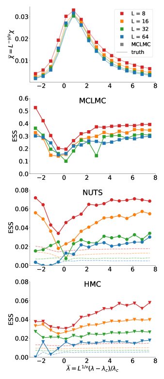
Figure 1: Top: susceptibility in the vicinity of the phase transition. We follow Gerdes et al. (2022) and rescale the susceptibility and the quartic coupling by the Ising model critical exponents $\nu=1$, $\gamma=7/4$ and the critical coupling $\lambda_{C}=4.25$ from Vierhaus (2010). The rescaling removes most of the lattice size dependence (Goldenfeld, 2018). MCLMC agrees with a long NUTS chain. The errors in the ESS estimations are negligible and therefore not displayed. 2nd panel: effective sample size (ESS) per action gradient evaluation for MCLMC. Higher is better. MCLMC tuning cost is included. 3rd panel: same for NUTS. Bottom: same for HMC. The dotted lines are the corresponding results if the tuning cost of 500 warm-up samples is taken into account.

We compare the results to standard HMC (Duane et al., 1987) and to a self-tuned HMC variant NUTS (Hoffman et al., 2014), both implemented in NumPyro (Phan et al., 2019). For HMC, we find that the optimal number of gradient calls between momentum resamplings to be 20, 30, 40 and 50 for lattice sizes $L=\,$ 8, 16, 32 and 64. The step size is determined with the dual averaging algorithm, which targets the average acceptance rate of 0.8 (NumPyro default), which adds considerably to the overall cost (Figure 1).

The results for grid sizes from $L=\,$8, 16, 32 and 64 are shown in Figure 1. The results for all samplers are computed with an annealing scheme: starting at high $\lambda$ and using the final state of the sampler as an initial condition at the next lowest $\lambda$ level. The initial condition at the highest $\lambda$ level is a random draw from the standard normal distribution on each lattice site. There is a near perfect agreement between a very long NUTS run (denoted as truth) and MCLMC in terms of susceptibility, where we observe a second order phase transition around the rescaled $\bar{\lambda}\sim 1$. Above the phase transition, ESS for MCLMC and HMC is relatively constant with $\bar{\lambda}$. ESS for NUTS and HMC scales with $L$ as $d^{-1/4}=L^{-1/2}$, as expected from adjusted HMC Neal et al. (2011). At the phase transition, NUTS and HMC suffer from the critical slowing down, resulting in lower ESS. In contrast, ESS for MCLMC is almost independent of $\bar{\lambda}$ and $L$. Overall, MCLMC outperforms HMC and NUTS by 10-100 at $L=64$ if HMC and NUTS tuning is not included, and by at least 40 if tuning is included (MCLMC auto-tuning is cheap and included in the cost, and we use the recommended 500 warm up samples for tuning of NUTS and HMC). We thus expect that for $d=10^{8}$, typical of state-of-the-art lattice quantum chromodynamics calculations, the advantage of MCLMC over HMC and NUTS will be 2–3 orders of magnitude due to $d^{1/4}$ scaling. MCLMC also significantly outperforms recently proposed Normalizing Flow (NF) based samplers (Albergo et al., 2019; Gerdes et al., 2022). NFs scale poorly with dimensionality, and the training time increases by about one order of magnitude for each doubling of $L$, e.g. of order 10 hours for $L=32$ to reach 90% acceptance, and 60 hours to reach 60% acceptance at $L=64$ (Gerdes et al., 2022). In contrast, the wall-clock time of MCLMC at $L=64$ on a GPU is a fraction of a second, while even at $L=8096$ (completely out of reach of current NF based samplers) it is only 15 seconds.

VIII Conclusions

We introduced an energy conserving stochastic Langevin process in the continuous time limit that has no damping, and derived the corresponding Fokker-Planck equation. Its equilibrium solution is microcanonical in the total energy, yet its space distribution equals the desired target distribution given by the action, showing that the framework of Ma et al. (2015) is not a complete recipe of all SDEs whose equilibrium solution is the target density. MCLMC is also of practical significance: we have shown that it vastly outperforms HMC on a lattice $\phi^{4}$ model. HMC is currently the state-of-the-art integrator for lattice quantum chromodynamics Gattringer and Lang (2009); Degrand and DeTar (2006), a field where the computational demands are particularly intensive. Numerical results presented here suggest that MCLMC could offer significant improvements over HMC in the setting of high dimensional lattice models.

Acknowledgments: We thank Julian Newman for proving lemmas 3 and 5 and Qijia Jiang for useful discussions. This material is based upon work supported in part by the Heising-Simons Foundation grant 2021-3282 and by the U.S. Department of Energy, Office of Science, Office of Advanced Scientific Computing Research under Contract No. DE-AC02-05CH11231 at Lawrence Berkeley National Laboratory to enable research for Data-intensive Machine Learning and Analysis.

Appendix A

We here include a supplementary lemma, needed in the proof of lemma 3:

Lemma 5.

Let $M$ be a $C^{1}$ manifold. Let $(I,\mathcal{I},\mu)$ and $(J,\mathcal{J},\nu)$ be probability spaces, and over these probability spaces respectively, let $(\Phi_{\alpha})_{\alpha\in I}$ and $(\Psi_{\beta})_{\beta\in J}$ be random $C^{1}$ self-embeddings of $M$. Fix $x_{1},x_{2}\in M$, let $p$ be the law over $\mu$ of $\alpha\mapsto\Phi_{\alpha}(x_{1})$, and let $\tilde{p}$ be the law over $\mu\otimes\nu$ of $(\alpha,\beta)\mapsto\Psi_{\beta}(\Phi_{\alpha}(x_{1}))$. Suppose there exists $m>0$ and an open subset $U$ of a chart on $M$ such that

• for every $A\in\mathcal{B}(U)$, $p(A)\geq m\operatorname{Leb}(A)$;

• $\nu(\beta\in J|x_{2}\in\Psi_{\beta}(U))>0$.

Then there exists $\tilde{m}>0$ and a neighborhood $\tilde{U}$ of $x_{2}$ contained in a chart on $M$ such that for every $A\in\mathcal{B}(\tilde{U})$, $\tilde{p}(A)\geq\tilde{m}\operatorname{Leb}(A)$.

Proof.

One can find a $\nu$-positive measure set $J^{\prime}\subset J$, a neighborhood $\tilde{U}$ of $x_{2}$ contained in a chart on $M$, and a value $r>0$, such that for all $\beta\in J^{\prime}$ and $x\in\tilde{U}$, we have $\Psi^{-1}_{\beta}(x)\in U$ and $|\operatorname{det}(D(\Psi^{-1}_{\beta})(x))|\geq r$. Now take any $A\in\mathcal{B}(\tilde{U})$ and let

$$E=\{(\alpha,\beta)\in I\times J^{\prime}|\Psi_{\beta}(\Phi_{\alpha}(x_{1}))\in A\}$$

then

$$\tilde{p}(A) \geq(\mu\otimes\nu)(E)=\int_{J^{\prime}}\mu(\alpha\in I|\Psi_{\beta}(\Phi_{\alpha}(x_{1}))\in A)\,\nu(d\beta)$$

$$=\int_{J^{\prime}}p(\Psi^{-1}_{\beta}(A))\,\nu(d\beta)\geq m\int_{J^{\prime}}\operatorname{Leb}(\Psi^{-1}_{\beta}(A))\,\nu(d\beta)$$

$$\geq m\nu(J^{\prime})r=\tilde{m}\operatorname{Leb}(A).$$

Therefore, $\tilde{p}(A)\geq\tilde{m}\operatorname{Leb}(A).\quad\blacksquare$ ∎

References

- Leimkuhler and Matthews (2015) B. Leimkuhler and C. Matthews, Interdisciplinary applied mathematics 36 (2015).
- Duane et al. (1987) S. Duane, A. D. Kennedy, B. J. Pendleton, and D. Roweth, Physics letters B 195, 216 (1987).
- Metropolis et al. (2004) N. Metropolis, A. W. Rosenbluth, M. N. Rosenbluth, A. H. Teller, and E. Teller, The Journal of Chemical Physics 21, 1087 (2004), ISSN 0021-9606, eprint https://pubs.aip.org/aip/jcp/article-pdf/21/6/1087/8115285/1087_1_online.pdf, URL https://doi.org/10.1063/1.1699114.
- Riou-Durand and Vogrinc (2022) L. Riou-Durand and J. Vogrinc, Metropolis adjusted langevin trajectories: a robust alternative to hamiltonian monte carlo (2022), eprint 2202.13230.
- Ma et al. (2015) Y. Ma, T. Chen, and E. B. Fox, in Advances in Neural Information Processing Systems 28: Annual Conference on Neural Information Processing Systems 2015, December 7-12, 2015, Montreal, Quebec, Canada, edited by C. Cortes, N. D. Lawrence, D. D. Lee, M. Sugiyama, and R. Garnett (2015), pp. 2917–2925.
- Ver Steeg and Galstyan (2021) G. Ver Steeg and A. Galstyan, Advances in Neural Information Processing Systems 34, 11012 (2021).
- Robnik et al. (2022) J. Robnik, G. B. De Luca, E. Silverstein, and U. Seljak, arXiv preprint arXiv:2212.08549 (2022).
- Elworthy (1998a) K. Elworthy, Probability towards 2000 pp. 165–178 (1998a).
- Elworthy (1998b) K. D. Elworthy, Stochastic differential equations on manifolds (Springer, 1998b).
- Baxendale (1991) P. H. Baxendale, Spatial Stochastic Processes: A Festschrift in Honor of Ted Harris on his Seventieth Birthday pp. 189–218 (1991).
- Kliemann (1987) W. Kliemann, The annals of probability pp. 690–707 (1987).
- Li and Erdogdu (2020) M. B. Li and M. A. Erdogdu, arXiv preprint arXiv:2010.11176 (2020).
- Øksendal and Øksendal (2003) B. Øksendal and B. Øksendal, Stochastic differential equations (Springer, 2003).
- Baras et al. (1990) J. S. Baras, V. Mirelli, et al., (No Title) (1990).
- Noorizadeh (2010) E. Noorizadeh (2010).
- Gattringer and Lang (2009) C. Gattringer and C. Lang, Quantum chromodynamics on the lattice: an introductory presentation, vol. 788 (Springer Science & Business Media, 2009).
- Vierhaus (2010) I. Vierhaus, Master’s thesis, Humboldt-Universität zu Berlin, Mathematisch-Naturwissenschaftliche Fakultät I (2010).
- Albergo et al. (2019) M. S. Albergo, G. Kanwar, and P. E. Shanahan, Physical Review D 100, 034515 (2019).
- Albergo et al. (2021) M. S. Albergo, D. Boyda, D. C. Hackett, G. Kanwar, K. Cranmer, S. Racaniere, D. J. Rezende, and P. E. Shanahan, arXiv preprint arXiv:2101.08176 (2021).
- Gerdes et al. (2022) M. Gerdes, P. de Haan, C. Rainone, R. Bondesan, and M. C. Cheng, arXiv preprint arXiv:2207.00283 (2022).
- Omelyan et al. (2003) I. Omelyan, I. Mryglod, and R. Folk, Computer Physics Communications 151, 272 (2003).
- Goldenfeld (2018) N. Goldenfeld, Lectures on phase transitions and the renormalization group (CRC Press, 2018).
- Hoffman et al. (2014) M. D. Hoffman, A. Gelman, et al., J. Mach. Learn. Res. 15, 1593 (2014).
- Phan et al. (2019) D. Phan, N. Pradhan, and M. Jankowiak, arXiv preprint arXiv:1912.11554 (2019).
- Neal et al. (2011) R. M. Neal et al., Handbook of markov chain monte carlo 2, 2 (2011).
- Degrand and DeTar (2006) T. A. Degrand and C. DeTar, Lattice methods for quantum chromodynamics (World Scientific, 2006).