Using inductive Energy Participation Ratio for Superconducting Quantum Chip Characterization

Abstract

We have developed an inductive energy participation ratio (iEPR) method and a concise procedure for superconducting quantum chip layout simulation and verification that is increasingly indispensable in large-scale, fault-tolerant quantum computing. It can be utilized to extract the characteristic parameters and the bare Hamiltonian of the layout in an efficient way. In theory, iEPR sheds light on the deep-seated relationship between energy distribution and representation transformation. As a stirring application, we apply it to a typical quantum chip layout, obtaining all the crucial characteristic parameters in one step that would be extremely challenging through the existing methods. Our work is expected to significantly improve the simulation and verification techniques and takes an essential step toward quantum electronic design automation.

Introduction

Benefiting from the rapid advance of micro-nano and manipulation technology, superconducting quantum chips have emerged as one of the most promising platforms for building quantum computers [1, 2, 3, 4, 5, 6]. Although significant progress [7, 8, 9, 10, 11, 12, 13, 14, 15, 16, 17] has been made, challenges remain on the way to large-scale and high-performance quantum chips. In addition to advanced fabrication technology, quantum electronic design automation (QEDA) is crucial yet often overlooked in the field. Similar to electronic design automation (EDA) in the conventional integrated circuit industry, QEDA is also highly desirable in developing large-scale, fault-tolerant quantum computers. It aims to simplify and optimize the process of quantum chip design and verification by providing a set of tools and methodologies. Among these core technologies, the indispensable part is simulation and verification, whose purpose is to capture the chip characteristics as accurate as possible and verify whether the design meets the demands. By doing so, the unnecessary trial-and-error costs in chip manufacturing will be reduced pronouncedly.

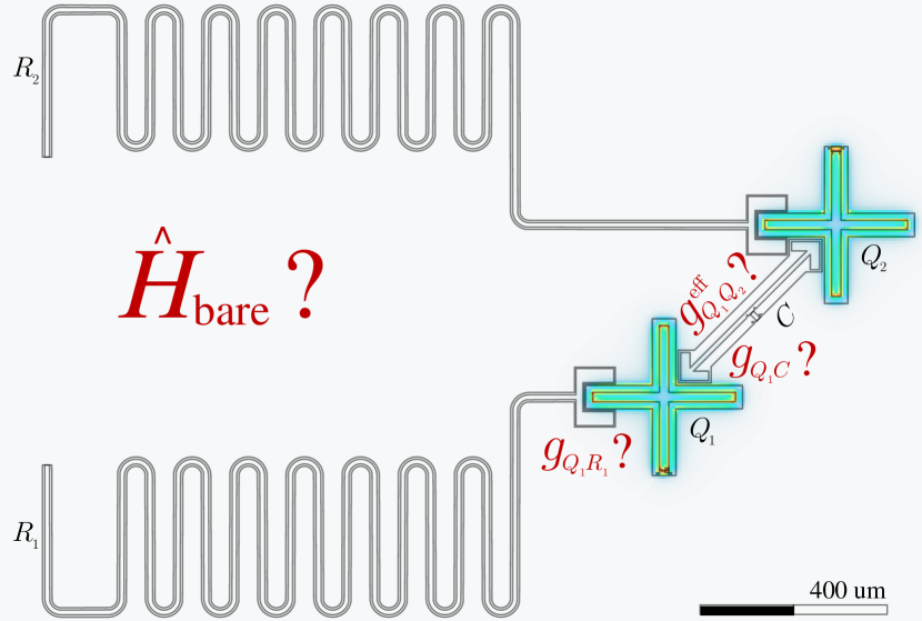
Figure 1: A typical quantum chip layout with superconducting coupler architecture. It consists of two qubits ($Q_{1},Q_{2}$), one coupler ($C$), and two resonators ($R_{1},R_{2}$). The electric field distribution can be evaluated via classical electromagnetic simulation. The key question addressed is how to work out efficiently the characteristic parameters of interest (e.g., the coupling strength between different elements) as well as the bare Hamiltonian $\hat{H}_{\rm bare}$ of the layout.

Let us start with a typical quantum chip layout of the attractive and widely used coupler architecture [1, 12, 5, 3, 2], as shown in Fig. 1. It consists of two qubits ($Q_{1}$, $Q_{2}$), one coupler ($C$), and two resonators ($R_{1}$, $R_{2}$). The non-trivial challenge addressed in this work is to extract the algebraic characteristic parameters (especially from the experimental interest) and the bare Hamiltonian from the geometric layout. Aside from the bare frequency of each element, obtaining the bare couplings among different elements is also essential. Since the spectrum of these couplings is broad, ranging from (near) resonant coupling (e.g., $Q_{1}$-$Q_{2}$ effective coupling) to dispersive coupling (e.g., $Q_{i}$-$R_{i}$ coupling, $i=1,2$, and $Q_{i}$-$C$ coupling)[18], characterizing the quantum chip layout entirely becomes an overwhelmingly tricky problem. Once obtaining the characterized parameters of interest, one is able to generate straightforwardly the layout’s bare Hamiltonian, which is thought of as “cumbersome and requires iteration between experiment and theory” [19]. With the bare Hamiltonian, all the system’s dynamical evolution can be predicted. Unfortunately, handling this issue is problematic because none of the existing methods fully meets the demand for accuracy, efficiency, and applicability in different coupling regimes.

To overcome the challenges, we developed a simple yet non-trivial method named “inductive Energy Participation Ratio (iEPR)”. Compared to the existing techniques, iEPR is applied to figure out all the characterized parameters and model the bare Hamiltonian of superconducting quantum chip layout in one step. Theoretically, we establish a fundamental connection between iEPR and unitary transformation, which bridges the bare mode Hamiltonian and normal mode Hamiltonian. Last but not least, we provide a practical and precise procedure to guide us to generate the bare Hamiltonian. This approach enables us to efficiently and accurately model the layout’s bare Hamiltonian, empowering researchers to verify and optimize the chip design before fabrication.

inductive Energy Participation Ratio (iEPR) method

The iEPR is defined as follows, which enables the quantitative generation of characteristic parameters and the bare Hamiltonian for a given superconducting quantum chip layout.

$$r_{mn}=\frac{\mathcal{E}_{mn}^{I}}{\mathcal{E}_{m}^{I}},$$ (1)

where the iEPR $r_{mn}$ represents the ratio of average inductive energy $\mathcal{E}_{mn}^{I}$ distributed in the $n$-th element to average inductive energy $\mathcal{E}_{m}^{I}$ stored in the full quantum chip when the normal mode $m$ is excited. Different from EPR method [20] which only collects the inductive energy stored in Josephson junctions, we found that the inductive energy of the entire element plays a vital role in generating the bare Hamiltonian. Both of these inductive energies can be extracted from classical electromagnetic (EM) simulation, from which the EM field distribution is evaluated (see Fig. 1). The main challenge addressed here is to generate the characteristic parameters and the bare Hamiltonian using the iEPR.

In the context of superconducting quantum chips integrating multiple qubits and coplanar resonators, a common model is a capacitively coupled system. Without loss of generality, the many-body Hamiltonian describing quantum chips is given by [21, 22, 23, 24]

$$\hat{H}_{\rm bare}=\sum_{m}\frac{\hat{Q}_{m}^{2}}{2C_{m}}+\frac{\hat{\Phi}_{m}^{2}}{2L_{m}}+\frac{1}{2}\sum_{m\neq n}\frac{C_{mn}}{C_{m}C_{n}}\hat{Q}_{m}\hat{Q}_{n},$$ (2)

where $\hat{Q}_{m}$ is the charge on the $m$-th capacitor with capacitance $C_{m}$, $\hat{\Phi}_{m}$ is the flux threading in the $m$-th element’s Josephson junctions or inductor with effective inductance $L_{m}$, and $C_{mn}$ is the mutual capacitance between the element $m$ and $n$. Note that the charge and flux variables are observables having the relation ($\hbar=1$ for simplicity) $[\hat{\Phi},\hat{Q}]=i$ [24]. To facilitate further analysis, we introduce an essential technique via using the following operator replacements: $\hat{\tilde{\Phi}}_{m}=\hat{\Phi}_{m}/\sqrt{L_{m}}$ and $\hat{\tilde{Q}}_{m}=\hat{Q}_{m}/(\omega_{m}\sqrt{C_{m}})$, where $\omega_{m}=1/\sqrt{L_{m}C_{m}}$ is the bare mode frequency of the $m$-th element. Then, the Hamiltonian (2) can be rewritten as $\hat{H}_{\rm bare}=\sum_{m}(\hat{\tilde{\Phi}}_{m}^{2}/2+\omega_{m}^{2}\hat{\tilde{Q}}_{m}^{2}/2)+\sum_{m\neq n}g_{mn}\sqrt{\omega_{m}\omega_{n}}\hat{\tilde{Q}}_{m}\hat{\tilde{Q}}_{n}$, with $g_{mn}=C_{mn}\sqrt{\omega_{m}\omega_{n}}/\left(2\sqrt{C_{m}C_{n}}\right)$ denoting the coupling strength. As a further step, we diagonalize the Hamiltonian via applying a unitary transformation $U$ as $\hat{H}_{\rm normal}=U\hat{H}_{\rm{bare}}U^{\dagger}=\sum_{m}\hat{\tilde{\Phi}}_{m}^{\prime 2}/2+\omega_{m}^{\prime 2}\hat{\tilde{Q}}_{m}^{\prime 2}/2$, where $\omega_{m}^{\prime}$ is the normal mode frequency. The vector space between bare mode representation $\bm{\Lambda}=(\hat{\tilde{\Phi}}_{1},\cdots,\hat{\tilde{\Phi}}_{m},\hat{\tilde{Q}}_{1},\cdots,\hat{\tilde{Q}}_{m})^{T}$ and normal mode representation $\bm{\Lambda}^{\prime}=(\hat{\tilde{\Phi}}^{\prime}_{1},\cdots,\hat{\tilde{\Phi}}^{\prime}_{m},\hat{\tilde{Q}}^{\prime}_{1},\cdots,\hat{\tilde{Q}}^{\prime}_{m})^{T}$ is also connected by the unitary transformation, namely $\bm{\Lambda}^{\prime}=U\bm{\Lambda}$. To ensure the commutation relationship is preserved as $[\hat{\tilde{\Phi}}_{m}^{\prime},\hat{\tilde{Q}}_{m}^{\prime}]=i$ after the transformation, the $U$ matrix has the block diagonal form $\mathcal{U}\oplus\mathcal{U}$, where $\mathcal{U}$ is also a unitary matrix with entry $u_{mn}$ [25]. In practical quantum chip layout simulation, although the normal mode information can be extracted conveniently using classical EM simulation, capturing the bare mode information (e.g., the coupling strength between different elements) is essential but not trivial. As the normal mode and bare mode representations are connected by $U$, then the critical question turns to how to figure out $U$ with the aid of the normal mode information. We will see iEPR is the key exactly.

Applying the definition of iEPR, namely Eq. (1), and using the bare Hamiltonian $\hat{H}_{\rm bare}$ and the normal Hamiltonian $\hat{H}_{\rm normal}$, we figure out a concise relation between iEPR $r_{mn}$ and unitary transformation $u_{mn}$. In particular, $r_{mn}={\langle\Psi_{m}^{\prime}|\hat{\tilde{\Phi}}_{n}^{2}/2|\Psi_{m}^{\prime}\rangle}/\sum_{k}{\langle\Psi_{m}^{\prime}|\hat{\tilde{\Phi}}_{k}^{\prime 2}/2|\Psi_{m}^{\prime}\rangle}$, where $|\Psi_{m}^{\prime}\rangle$ represents the eigenstate of the normal mode $m$. Note that the relation between $\hat{\tilde{\Phi}}_{n}$ and $\hat{\tilde{\Phi}}_{k}^{\prime}$ is govern by $\Lambda^{\prime}=U\Lambda$ referred before, from which one can obtain $\hat{\tilde{\Phi}}_{n}=\sum_{k}u_{kn}\hat{\tilde{\Phi}}_{k}^{\prime}$. Substituting the relation back, we ultimately obtain a concise result [25]

$$r_{mn}=u_{mn}^{2}.$$ (3)

To solve $u_{mn}$ from Eq. (3), we need an additional sign matrix $s_{mn}$, which can also be obtained from electromagnetic simulation. In the end, the matrix $U$ is expressed as

$$U=\begin{pmatrix}s_{11}\sqrt{r_{11}}&s_{12}\sqrt{r_{12}}&\cdots&s_{1n}\sqrt{r_{1n}}\\ s_{21}\sqrt{r_{21}}&s_{22}\sqrt{r_{22}}&\cdots&s_{2n}\sqrt{r_{2n}}\\ \vdots&\vdots&\ddots&\vdots\\ s_{n1}\sqrt{r_{n1}}&s_{n2}\sqrt{r_{n2}}&\cdots&s_{nn}\sqrt{r_{nn}}\end{pmatrix}^{\oplus 2}.$$ (4)

It reveals the profound relationship between iEPR and representation transformation. Because $\mathcal{U}$ is a unitary matrix, it is natural to obtain an orthonormality of iEPR as $\sum_{k}s_{nk}s_{mk}\sqrt{r_{nk}r_{mk}}=\sum_{k}s_{kn}s_{km}\sqrt{r_{kn}r_{km}}=\delta_{mn}$. Using classical EM simulation, the normal mode frequencies $\omega_{m}^{\prime}$, iEPR $r_{mn}$ and the sign matrix $s_{mn}$ can be calculated, which will be discussed later. Then the unitary transformation $U$ can be constructed by Eq. (4). Furthermore, we generate the bare Hamiltonian by applying $\hat{H}_{\rm bare}=U^{\dagger}\hat{H}_{\rm normal}U$. In particular, the bare mode frequency is evaluated as

$$\omega_{m}=\sqrt{\sum_{k}r_{km}\omega_{k}^{\prime 2}}$$ (5)

and the coupling strength is

$$g_{mn}=\frac{\sum_{k}s_{km}s_{kn}\sqrt{r_{km}r_{kn}}\omega_{k}^{\prime 2}}{2\sqrt{\omega_{m}\omega_{n}}}.$$ (6)

With the obtained bare mode characteristic parameters and after a second order quantization $\hat{\tilde{\Phi}}_{m}=\sqrt{\omega_{m}/2}\left(\hat{a}_{m}^{\dagger}+\hat{a}_{m}\right)$ and $\hat{\tilde{Q}}_{m}=i\sqrt{1/2\omega_{m}}\left(\hat{a}_{m}^{\dagger}-\hat{a}_{m}\right)$, the bare Hamiltonian is rewritten as

$$\hat{H}_{\rm bare}=\sum_{m}\omega_{m}\hat{a}_{m}^{\dagger}\hat{a}_{m}-\sum_{m\neq n}\frac{g_{mn}}{2}\left(\hat{a}_{m}^{\dagger}-\hat{a}_{m}\right)\left(\hat{a}_{n}^{\dagger}-\hat{a}_{n}\right)$$ (7)

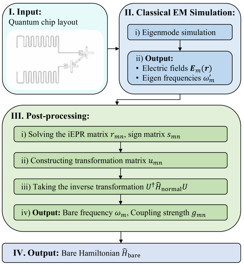
Figure 2: The procedure for quantum chip simulation and verification. Following this workflow, the characteristic parameters and the bare Hamiltonian of superconducting quantum chip layouts are generated automatically and efficiently.

Procedure for quantum chip simulation and verification

Based on the iEPR method, we further build a procedure that is expected to guide the quantum chip simulation and verification. In particular, the procedure (see Fig. 2) starts with a given superconducting quantum chip layout and ends with the characteristic parameters as well as the bare Hamiltonian. In particular, the process are divided into two main parts: classical EM simulation and post-processing. Firstly, the classical EM simulation is performed by doing eigenmode simulation via solving the three-dimensional Helmholtz equation of the quantum chip model. At the end, it outputs eigen frequencies $\omega_{m}^{\prime}$ and the electric field $\bm{E}_{m}(\bm{r})\cos(\omega_{m}^{\prime}t)$ of each normal mode $m$, where $\bm{E}_{m}(\bm{r})$ is the electric field amplitude (peak value) at position $\bm{r}$.

Method	iEPR[This work]	LC[26, 27, 28, 29, 30, 31]	BBQ[19, 32, 33]	EPR[20]	NMS[34]
Type of generated $\hat{H}$	bare & normal	bare & normal	normal	normal	N/A
Accuracy	high	low	high	high	high
Speed	moderate	high	low	moderate	low

Table 1: Comparison of various quantum chip simulation and verification methods. The iEPR shows unique and pronounced advantages compared with the existing methods. It can be used to generate efficiently the characteristic parameters of interest and the bare Hamiltonian from the quantum chip layout under different coupling regimes.

Next, let us enter the post-processing part. It deals with the essential task that how to extract the characteristic parameters in bare mode representation from the classical EM simulation. Recalling the definition of the iEPR, i.e., Eq. (1), both the average inductive energy stored in the full quantum chip and the specific element have to be calculated respectively. Actually, the evaluation of inductive energy stored in the full chip is equivalent to calculating the average electric field energy [20]. In particular, it can be solved by integrating the electric field in space over the entire volume of the quantum chip, given by $\mathcal{E}_{m}^{I}=\mathcal{E}_{m}^{E}=\int_{v_{\rm full}}[\epsilon(\bm{r})|\bm{E}_{m}(\bm{r})|^{2}/4]dv$, where $\epsilon(\bm{r})$ is the permittivity at position $\bm{r}$. It becomes challenging when it comes to determine the local inductive energy of a specific element. As an alternative technique, we employ an insightful approach, the inductive energy is linearly related to the power of flux passing through the element. Therefore, the average inductive energy stored in the specific elements is evaluated as $\mathcal{E}_{mn}^{I}=\Phi_{mn}^{2}/4L_{n}=V_{mn}^{2}/(4L_{n}\omega_{m}^{\prime 2})$ [25], where $\Phi_{mn}$ is the peak value of flux and $V_{mn}$ is the peak value of voltage across the $n$-th inductor of the element under mode $m$, $L_{n}$ is the inductance of $n$-th element. The peak voltage is evaluated as $V_{mn}=\int_{\bm{l}_{n}}\bm{E}_{m}(\bm{r})d\bm{l}$, where the integral path $\bm{l}_{n}$ is set between two potential nodes along the element [25]. Using Eq. (1), the iEPR is evaluated as $r_{mn}=[V_{mn}^{2}/(4L_{n}\omega_{m}^{\prime 2})]/\mathcal{E}_{m}^{I}$. By leveraging the orthonormality of the iEPR matrix derived earlier, $\sum_{m}r_{mn}=\sum_{m}[V_{mn}^{2}/(4L_{n}\omega_{m}^{\prime 2})]/\mathcal{E}_{m}^{I}=1$, we obtain the phenomenological parameter $L_{n}=\sum_{m}(V_{mn}^{2}/\omega_{m}^{\prime 2})/4\mathcal{E}_{m}^{I}$ and subsequently the iEPR:

$$r_{mn}=\frac{V_{mn}^{2}/(\omega_{m}^{\prime 2}\mathcal{E}_{m}^{I})}{\sum_{k}V_{kn}^{2}/(\omega_{k}^{\prime 2}\mathcal{E}_{k}^{I})}.$$ (8)

In the denominator of the equation above, $k$ represents the index of different modes, and the summation includes the iEPR values for element $n$ across these modes. Since $L_{n}$ is a phenomenological parameter obtainable from the energy distribution, iEPR method is versatile and can be extended to all inductive elements, unlike the EPR method [20], which is limited to scenarios where the element’s inductance is known. Moreover, from Eq. (3), we know that $u_{mn}$ is related to ${\langle\Psi_{m}^{\prime}|\hat{{\Phi}}_{n}|\Psi_{m}^{\prime}\rangle}\propto\Phi_{mn}$, so the sign $s_{mn}$ depends on $\Phi_{mn}$, which is also equivalent to the sign of $V_{mn}$ [25]. After defining the reference oriented line segment and obtaining the electric field distribution, we can ascertain the sign of $s_{mn}$ in the transformation matrix. With the crucial pieces of information, $r_{mn}$ and $s_{mn}$, at our disposal, we can reconstruct the transformation matrix $U$. Subsequently, this allows us to determine all of the bare frequency and coupling strength, culminating in the derivation of the bare Hamiltonian.

Features of the iEPR method

Compared with the existing methods [26, 27, 28, 29, 30, 31, 19, 32, 33, 20, 34], iEPR method shows the unique and pronounced advantages, as summarized in Tab. 1. The iEPR method, which relies on classical full-wave eigenmode EM simulation, offers high accuracy at a moderate speed. Its versatility lies in the fact that it can work in any coupling regime and provide relative positive and negative coupling strengths, making it a unique methodology for superconducting quantum chip characterization. As a comparison, other existing methods display their own merits and demerits. In particular, i) The lumped circuit (LC) method [26, 27, 28, 29, 30, 31] is efficient and adaptive in any coupling regime, but the results’ accuracy is restricted by the static EM simulation technique; ii) The black-box quantization (BBQ) method [19, 32, 33] has a relatively higher accuracy benefiting from the full-wave driving mode EM simulation technique (with a slower speed) but is only suitable for normal mode representation; iii) The energy participation ratio (EPR) method [20] has to satisfy the same restrictions as BBQ. Compared with LC and BBQ, it provides a balance between accuracy and speed with the aid of a full-wave eigenmode simulation technique; iv) The normal modes simulation (NMS) method [34] is only valid for resonant coupling regime, beyond which the speed is lower because a large number of simulated data is required. Obviously, most of the methods used to study coupled systems focus on normal modes, which represent the collective oscillations of the system as a whole [34]. However, the bare modes, which reflect the properties of individual elements and their direct coupling, are absent. The iEPR method opens a new possibility for exploring characteristics in bare-mode representations.

Applications and Discussion

To demonstrate the effectiveness and advantages of the iEPR method and the procedure, we apply them to the quantum chip layout shown in Fig. 1. To generate the bare Hamiltonian of the layout, we have to at least determine, i) the bare frequencies of qubit, coupler and resonator; ii) the coupling strength (dispersive type) between qubit and resonator; iii) the coupling strength (dispersive type) between qubit and coupler; iv) the direct coupling strength (resonant type) between two qubits. As the two-qubit gate fidelity is highly related to the effective coupling between the two qubits, v) we also need to work out the qubit-qubit effective coupling (resonant type) characteristics.

To solve these concerned parameters, the procedure (i.e., Fig. 2) is implemented step by step to the layout. In particular, we perform the classical EM simulation by setting the layout size as $\rm 10.1\,mm\times 10.1\,mm$, and the substrate material is chosen as sapphire with the relative permittivity as $\rm{10.5}$, and thickness as $\rm 500\ \mu m$. In the end, the interested characteristic parameters are solved and presented in Tab. 2. As seen from the table, the diagonal term represents the bare frequency of the qubit, coupler, and resonator, respectively; and the coupling between different elements is described by the off-diagonal term. With these parameters, we are able to generate the bare Hamiltonian of the layout of interest, and further, acquire its dynamical evolution. It is worth pointing out that all the characteristic parameters in the table are worked out in one step, which means one only has to perform one-time EM simulation. To our knowledge, no existing method can complete this task with high accuracy, much less generate them in one step.

	$Q_{1}$	$Q_{2}$	$C$	$R_{1}$	$R_{2}$
$Q_{1}$	$6699.37$	$8.76$	$158.05$	$40.08$	$1.33$
$Q_{2}$	$8.76$	$6701.12$	$159.92$	$0.37$	$40.56$
$C$	$158.05$	$159.92$	$8118.31$	$1.68$	$14.00$
$R_{1}$	$40.08$	$0.37$	$1.68$	$5019.11$	$0.36$
$R_{2}$	$1.33$	$40.56$	$14.00$	$0.36$	$5092.84$

Table 2: The characteristic parameters of the layout of interest solved using the procedure. The unit of all the parameters is MHz. The diagonal term represents the bare frequency of each element, while the off-diagonal term describes the coupling strength between different elements.

In addition to the critical parameters, one more vital task is qubit-qubit effective coupling characteristics [1, 12, 5, 3, 2]. In coupler architecture, one key feature is that the effective coupling between adjacent qubits can be tuned from positive to negative by manipulating the coupler frequency [35]. For EM simulation experiments, this can be realized by varying the effective inductance of the coupler. Although the layout contains five elements, we do not have to consider all the possible modes that are necessary yet complicated for $\rm{LC}$ method. Instead, we only have to focus on the two modes related to qubits, from which the effective coupling is solved conveniently; the rationality of reducing the many-body problem to a two-body system has been verified [25]. Again, following the procedure given in Fig. 2 with varying coupler inductance $L_{C}^{\rm J}$, we solve and show the qubit-qubit effective coupling characteristics in Fig. 3(a). It is seen that the effective coupling strength predicted using the iEPR method goes from positive to negative with increasing the coupler inductance, and the coupling is switched off around $2.3~{}{\rm nH}$. We verify the iEPR results (blue solid) using two existing methods: NMS (orange dash-dotted) and LC (red dotted), while BBQ and EPR methods are incapable of action unfortunately on this important issue. The consistency between iEPR and the other two methods reveals the effectiveness of the iEPR method and the procedure for quantum chip simulation and verification. Next, let us add some remarks to the three different methods. Since the sign of the coupling strength can not be determined by NMS method, justifying the “switch-off” property of the coupler architecture becomes a difficult problem. The LC method faces great challenges with an increasing number of the qubit integrating on the quantum chip. Nevertheless, the iEPR method does not suffer from these and displays pronounced advantages.

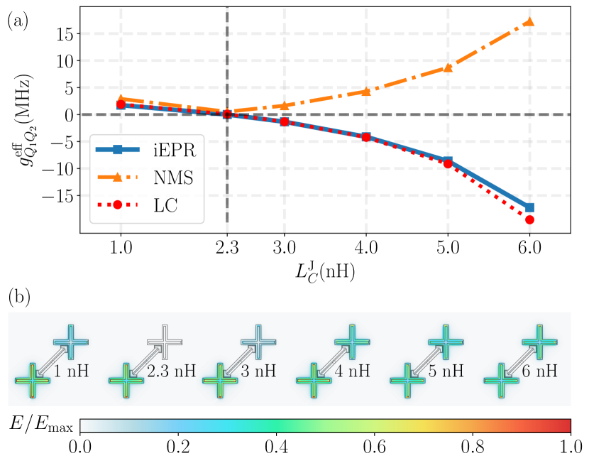
Figure 3: (a) Qubit-Qubit effective coupling characteristics. With varying the coupler inductance $L_{C}^{J}$, the effective coupling strength $g_{Q_{1}Q_{2}}^{\rm eff}$ is tuned from positive to negative, and across zero around $2.3\,\rm{nH}$. The results obtained using iEPR method (blue solid) are verified simultaneously using NMS method (orange dash-dotted) and LC method (red dotted). (b) The electric field distribution $E$ (normalized by the maximum $E_{\rm max}$) of the qubit mode corresponding to different $L_{C}^{J}$ in (a).

Last but not least, we found an insightful correspondence between the electric field distribution of the qubit mode and the qubit-qubit effective coupling characteristics. As shown in Fig. 3(b), when the electric field isolates on a single qubit, e.g., at $2.3\,{\rm nH}$, implies the qubit does not interact with each other, hence corresponding to the “switch-off” point (zero coupling). As a comparison, the strong effective coupling is generated when the electric field is distributed in both of the qubits, meaning the qubits couple strongly with each other. This correspondence reveals the profound relation between the inductive energy participation ratio and the coupling characteristics. Indeed, this intuitive finding exactly inspires this work. Eventually, we not only provide a complete theoretical explanation of this marvelous correspondence but also present quantitative and precise results.

Summary and Outlook

In summary, we introduced the iEPR method as well as the simulation and verification procedure to characterize superconducting quantum chips. While other existing methods face different challenges, the iEPR method has the unique advantage of generating the characteristic parameters of interest and the bare Hamiltonian in an efficient way; and we demonstrate it in the practical coupler architecture. Looking forward, other interesting issues such as the coupling between the parasitic mode and the element mode [36], the cross-talk problem [37, 38, 39], as well as the surface loss issue [40] may be studied using the iEPR method. Benefiting from the well-defined procedure, we provide a powerful methodology for simulation and verification in the quantum chip design, taking an important step towards superconducting quantum electronic design automation.